Finding the right XAI method — A Guide for the Evaluation and Ranking of Explainable AI Methods in Climate Science

Abstract

Explainable artificial intelligence (XAI) methods shed light on the predictions of deep neural networks (DNNs). Several different approaches exist and have partly already been successfully applied in climate science. However, the often missing ground truth explanations complicate their evaluation and validation, subsequently compounding the choice of the XAI method. Therefore, in this work, we introduce XAI evaluation in the context of climate research and assess different desired explanation properties, namely, robustness, faithfulness, randomization, complexity, and localization. To this end we build upon previous work and train a multi-layer perceptron (MLP) and a convolutional neural network (CNN) to predict the decade based on annual-mean temperature maps. Next, multiple local XAI methods are applied and their performance is quantified for each evaluation property and compared against a baseline test. Independent of the network type, we find that the XAI methods Integrated Gradients, Layer-wise relevance propagation, and InputGradients exhibit considerable robustness, faithfulness, and complexity while sacrificing randomization. The opposite is true for Gradient, SmoothGrad, NoiseGrad, and FusionGrad. Notably, explanations using input perturbations, such as SmoothGrad and Integrated Gradients, do not improve robustness and faithfulness, contrary to previous claims. Overall, our experiments offer a comprehensive overview of different properties of explanation methods in the climate science context and supports users in the selection of a suitable XAI method.

Introduction

Deep learning (DL) has become a widely used tool in climate science and assists various tasks, such as Nowcasting (Shi et al., 2015; Han et al., 2017; Bromberg et al., 2019), climate or weather monitoring (Hengl et al., 2017; Anantrasirichai et al., 2019) and forecasting (Ham et al., 2019; Chen et al., 2020; Scher and Messori, 2021), numerical model enhancement (Yuval and O’Gorman, 2020; Harder et al., 2021) and up-sampling of satellite data (Wang et al., 2021; Leinonen et al., 2021). However, a deep neural network (DNNs) is mostly considered a black-box due to its inaccessible decision-making process. In climate research, the DNNs’ lack of transparency further increases skepticism towards DL in general and can discourage their application (McGovern et al., 2019; Camps-Valls et al., 2020; Sonnewald and Lguensat, 2021; Clare et al., 2022). For DNNs to be considered trustworthy, they should not only have a high predictive performance (e.g., high accuracy) but further provide accessible predictive reasoning consistent with existing theory (Commission et al., 2019; Thiebes et al., 2020).
The field of explainable artificial intelligence (XAI) enables a deeper understanding of DL methods by explaining the reasons behind the predictions of a network. In the climate context, XAI can validate DNNs and provide researchers with new insights into physical processes (Ebert-Uphoff and Hilburn, 2020; Hilburn et al., 2021). For example, Gibson et al. (2021) could demonstrate by using XAI that DNNs produce skillful seasonal precipitation forecasts based on relevant physical processes. Moreover, XAI proved useful for the forecasting of drought (Dikshit and Pradhan, 2021), of teleconnections (Mayer and Barnes, 2021), and of precipitation in the United States (Pegion et al., 2022), and was used to assess external drivers of global climate change (Labe and Barnes, 2021) and to understand sub-seasonal drivers of high-temperature summers (van Straaten et al., 2022). (Labe and Barnes, 2022) even showed that XAI applications can aid in the comparative assessment of climate models.
As the number of XAI methods increases, choosing the right method for a specific task becomes more opaque. Generally, XAI can be categorized using three aspects (Letzgus et al., 2022; Mamalakis et al., 2021). The first considers local and global decision-making as well as self-explaining models. Local explanations provide explanations of the network decision for individual samples (Baehrens et al., 2010; Bach et al., 2015; Vidovic et al., 2016; Ribeiro et al., 2016), e.g., by assessing the contribution of each pixel in a given image based on the predicted class. In contrast, global explanations reveal the overall decision strategy, e.g. by showing a map of important features or image patterns that were learned by the model for the whole class (Simonyan et al., 2014; Nguyen et al., 2016; Vidovic et al., 2015; Lapuschkin et al., 2019; Grinwald et al., 2022; Bykov et al., 2021). Self-explaining models, such as Chen et al. (2019); Gautam et al. (2023, 2022) base their decisions on an additional prototype layer after the convolutional layers, which is transparent and comprehensible in itself. As a second aspect, the information that is used by the XAI method is considered and one differentiates between model-aware and model-agnostic methods. The former use components of the trained model, such as network weights, for the explanation calculation, while model-agnostic methods consider the model as a black-box and only assess the change in the output caused by a perturbation in the input (Strumbelj and Kononenko, 2010; Ribeiro et al., 2016). The last aspect considers the output of the explanation, which can differ in terms of meaning — explanations, such as absolute gradient can be interpreted as showing the intensity of a feature, e.g. pixel, regarding a certain prediction, whereas explanation methods, such as Layer-wise Relevance Propagation add information to each feature as to whether it contributed positively or negatively to predicting the class. In climate research, the decision pattern learned by DNNs is mostly visualized with local explanation methods (Gibson et al., 2021; Dikshit and Pradhan, 2021; Mayer and Barnes, 2021; Labe and Barnes, 2021, 2022). Nonetheless, different local XAI methods can identify different input features as relevant to the network decision, subsequently leading to different scientific conclusions. While there might be particular XAI properties beneficial for the application at hand, practitioners often choose an explanation method based upon popularity or upon easy-access (Krishna et al., 2022). To navigate the field of XAI, recent publications in climate science have compared and assessed different explanation techniques using benchmark datasets with accessible target explanations (Mamalakis et al., 2021, 2022). This resembles the calculation of the network performance by comparing predictions with a defined target, considered as ground truth. However, the target explanations are derived from the model, which was used to generate the dataset not from the trained model, and therefore can only be considered as approximations of the ground truth (Mamalakis et al., 2021).

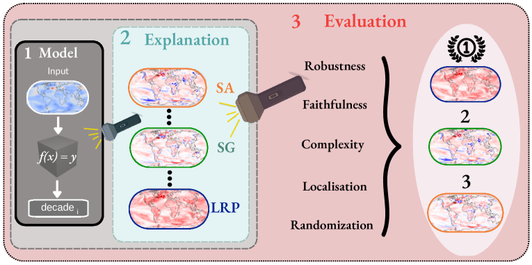
Figure 1: Schematic of the XAI evaluation procedure. Given a network decision (box $1$), the explanation methods (SA - Salieny or Gradient, SG - SmoothGrad, LRP - Layer-wise relevance propagation) enable insights (shine a light - box $2$) into the specific decision. The explanation maps of the model decision, for 3 different XAI methods (marked in orange, green and blue) highlight different areas as positively (red) and negatively (blue) contributing to the network decision. To ’shine a light’ on the different explanation methods and subsequently support an appropriate choice (here indicated by the first rank), we can use XAI evaluation to assess robustness, faithfulness, localisation, complexity, and randomisation properties of the explanations.

In general, XAI lacks ground truth explanations for a proper quantitative evaluation. Therefore, the field of XAI was expanded by the area of XAI evaluation, where metrics are developed for measuring the relieability of an explanation based on different properties. In this work, we introduce XAI evaluation in the context of climate science to compare different explanation methods of commonly used models, i.e., CNN and MLP. XAI evaluation quantitatively assesses the robustness, complexity, localization, randomization and faithfulness properties of explanation methods, thereby making XAI methods comparable and successively enabling their ranking based on the desired properties for specific tasks (Hoffman et al., 2018; Arrieta et al., 2020; Mohseni et al., 2021; Hedström et al., 2023).

Here we build upon previous research (Labe and Barnes, 2021) and train a model based on 2m-temperature maps to predict the respective decade (see step 1 in Figure 1 which illustrates this workflow schematically). To make the decision comprehensible, we apply several explanation methods, which vary in their explained evidence and might lead to different conclusions (step 2 in Figure 1). Therefore, in the next step, we apply XAI evaluation techniques (Hedström et al., 2023) to quantitatively measure the reliability of the different XAI methods (step 3 in Figure 1), rank them, and provide statements about the respective suitability for the underlying climate task.

This paper is structured as follows. In Section 2 we introduce the dataset, the different network types, i.e., MLP and CNN, as well as the different explanation methods. Moreover, we provide a detailed description of XAI evaluation and the assessed five evaluation properties. Then, in Section 34.1 we discuss the performance of both networks and provide an example highlighting the risks of an uninformed choice of an explanation method. In Section 4.2, we use a random baseline test to assess the evaluation metrics’ compatibility with climate data properties for two metrics in each evaluation property. We then discuss the implications of the evaluation properties in the climate context and establish an evaluation guideline based on compatible metrics. In Section 4.3 we rank the performance of the XAI methods in each property based on their evaluation scores. We compare the rankings for the MLP and CNN. Finally, in section 4.4 we present a guideline on using XAI evaluation to choose an optimal explanation and discuss our results and state our conclusions in Section 5.

Data and Methods

2.1 Data

Following Labe and Barnes (2021), we use data simulated by the general climate model, CESM1 (Hurrell et al., 2013), focusing on the “ALL” configuration (Kay et al., 2015), which is discussed in detail in Labe and Barnes (2021). We use the global $2$-m air temperature (T2m) temperature maps from $1920$ to $2080$. The data $\bm{\Omega}$ consist of $\mathrm{I}=40$ ensemble members $\Omega_{i\in\{1,\dots,I\}}$ and each member is generated by varying the atmospheric initial conditions $z_{i}$ with fixed external forcing $\theta_{\mathrm{clima}}$. Following Labe and Barnes (2021), we compute annual averages and apply a bilinear interpolation. This results in $T=161$ temperature maps for each member $\Omega_{i}\in\mathbb{R}^{vxhxT}$, with $v=144$ and $h=95$ denoting the number of longitude and latitude, with $1.9^{\circ}$ sampling in latitude and $2.5^{\circ}$ sampling in longitude. The temperature maps $x\in\Omega\in\mathbb{R}^{vxh}$ are finally standardized by removing the multi-year $1920-2080$ mean and by subsequently dividing by the corresponding standard deviation.

2.2 Networks

Following Labe and Barnes (2021) we train an MLP to solve a fuzzy classification problem by combining classification and regression. The MLP can be defined as a function $f_{\text{MLP}}:\mathbb{R}^{d}\rightarrow\mathbb{R}^{c}$ with network weights $W\in\mathcal{W}$. As input $\mathbf{x}\in\Omega$, the network considers the flattened temperature maps with $d=v\times h$. First, in the classification setting, the network assigns each map to one of the $C=20$ different classes, where each class corresponds to one decade (see Figure 1 in Labe and Barnes (2021)). The network output $f(x)$, thus, is a probability vector $\mathbf{y}\in\mathbb{R}^{1\times C}$ across $C=20$ classes. Afterwards, since the network can assign a nonzero probability to more than one class, regression is used to predict the year $\hat{y}$ of the input as:

$$\hat{y}=\sum_{i=1}^{C}y_{i}\bar{Y}_{i},$$ (1)

where $y_{i}$ is the probability of class $i$, predicted by the network $\mathbf{y}=f(\mathbf{x})$ in the classification step and $\bar{Y}_{i}$ denotes the central year of the corresponding decade class $i$ (e.g. for class $i=1$, $\bar{Y}_{1}=1925$ represents the decade $1920-1929$). Note that, in this work, we focus on the class prediction of the network and use the regression only for performance evaluation (following Labe and Barnes (2021)).

Additionally, we construct a convolutional neural network (CNN) of comparable size (three times the number of parameters compared to the MLP). This network $f_{\text{CNN}}:\mathbb{R}^{v\times h}\rightarrow\mathbb{R}^{c}$ consists of a 2D-convolutional layer (2dConv) with $6\times 6$ window size and a stride of 2. The second layer includes a max-pooling layer with a $2\times 2$ window size, followed by a dense layer with $L^{2}$-regularization and a softmax output layer. Unlike the flattened input used for the MLP, the CNN maintains the longitude-latitude grid of the data $\mathbf{x}_{\text{img}}\in\mathbb{R}^{v\times h}$ after pre-processing (see Section 2.1).
Similar to Labe and Barnes (2021), the datasets include a training $\Omega_{\mathrm{tr}}$ and a test set $\Omega_{\mathrm{test}}$ which we randomly sample. For both MLP and CNN we consider $20\%$ of the data as test set and the remaining $80\%$ is split into a training ($64\%$) and validation ($16\%$) set.

2.3 Explainable Artificial Intelligence (XAI)

In this work, we focus on commonly used model-aware explanation methods in climate science (Sonnewald and Lguensat, 2021; Mamalakis et al., 2021; Mayer and Barnes, 2021; Labe and Barnes, 2021, 2022; Mamalakis et al., 2022; Clare et al., 2022; Pegion et al., 2022), which we briefly present in the following (see Appendix A.1 for details). Note that we do not consider model-agnostic explanation methods, since the computational time rises with increasing dimensionality of the input data (Clare et al., 2022).

Gradient/Saliency (Baehrens et al., 2010)

explains the network decision by computing the first partial derivative of the network output $f(\mathbf{x})$ with respect to the input. This explanation method feeds backwards the network’s prediction to the features in the input $\mathbf{x}$, calculating the change in network prediction given a change in the respective features, which corresponds to the network function sensitivity.

InputGradient

is an extension of the gradient method and extends the information content towards the input image by computing the product of the gradient and the input. The explanation assigns a high relevance score to an input feature if it is both present in the data and if the model gradient reacts to it.

Integrated Gradients (Sundararajan et al., 2017)

extends InputGradients, by introducing a baseline datapoint (e.g. a zero or a mean centred image) and computes the explanation based on the difference to this baseline.

Layerwise Relevance Propagation(LRP) (Bach et al., 2015; Montavon et al., 2019)

computes the relevance for each input feature by feeding the network’s prediction backwards through the model, layer by layer. This back-propagation follows different rules. The main strategy mimics the energy conversation rule, meaning that the sum of all relevances within one layer is equal to the original prediction score—until the prediction score is distributed over the input features. The $\bm{\alpha}$-$\bm{\beta}$-rule, assigns the relevance at each layer to each neuron. All positively contributing activations of connected neurons in the previous layer are weighted by $\alpha$ and $\beta$ to determine the contribution of the negative activations. The default values are $\alpha=1$ and $\beta=0$, where only positively contributing activations are considered.
The z-rule calculates the explanation by including both negative and positive neuron activations. Hence, the corresponding explanations, visualized as heatmaps, display both positive and negative evidence. The composite-rule combines various rules for different layer types. The method accounts for layer structure variety in CNNs, such as fully-connected, convolutional and pooling layers (see Appendix A.1).

SmoothGrad (Smilkov et al., 2017)

aims to filter out the unwanted background noise (i.e., the gradient shattering effect) to enhance the interpretability of the explanation. To this end, random noise is added to the input and the model’s explanations are averaged over multiple noisy versions of the input. The idea behind the average across noisy inputs is that the noise-induced variations in the model’s explanation will on average highlight the most important features, while suppressing the background noise.

NoiseGrad (Bykov et al., 2022)

perturbs the weights of the model instead of the input feature as done by SmoothGrad. The multiple explanations, resulting from explaining the noisy versions of the model are averaged and aim to suppress the background noise of the image in the final explanation.

FusionGrad (Bykov et al., 2022)

combines SmoothGrad and NoiseGrad by perturbing both the input features and the network weights. The purpose of the method is to account for uncertainties within the network and the input space (Bykov et al., 2021).

Here we maintain literature values for most hyperparameters of the explanation methods (see Appendix B.1). An exception are hyperparameters of explanation methods requiring input perturbation, such as SmoothGrad and FusionGrad. We adjust the perturbation levels to the varying levels of the data to account for strong uncertainty as present in climate data.

Evaluation techniques

XAI research has developed metrics that assess different properties an explanation method should fulfill. These properties provide a categorisation of the XAI evaluation metrics and can serve to evaluate different explanation methods (Hoffman et al., 2018; Arrieta et al., 2020; Mohseni et al., 2021; Hedström et al., 2023). We follow Hedström et al. (2023) and analyze five different evaluation properties, as listed below. To create intuition, we provide a schematic diagram of each property (See Figures 2-6) based on the classification task from Labe and Barnes (2021).

3.1 Robustness

Robustness measures the stability of an explanation regarding small changes in the input image $\mathbf{x}+\delta$ (Alvarez-Melis and Jaakkola, 2018; Yeh et al., 2019; Montavon et al., 2018). Ideally, small changes ($\delta<\epsilon$) in the input sample should produces only small changes in the model prediction and successively only small changes in the explanation (see Figure 2).

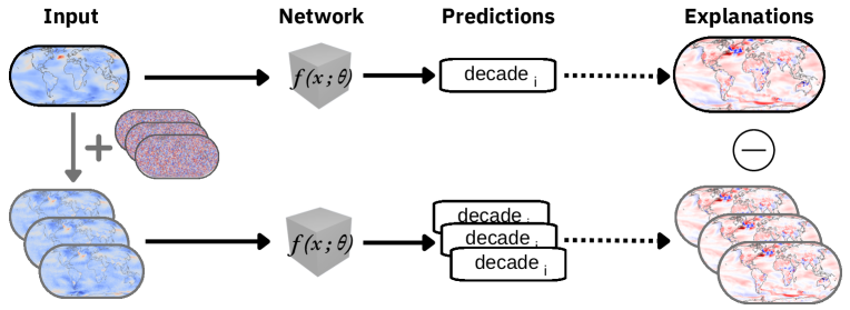
Figure 2: Diagram of the concept behind the robustness property. Perturbed input images are created by adding uniform noise maps of small magnitude to the original temperature map (left part of Figure). The perturbed maps are passed to the network, resulting in an explanation map for each prediction. The explanation maps of the perturbed inputs (explanation maps with grey outlines) are then compared to (indicated by minus sign) the explanation of the unperturbed input (explanation map with black outline). A robust XAI method is expected to produce similar explanations for the perturbed input and unperturbed inputs.

To measure robustness, we choose the Local Lipschitz estimate (Alvarez-Melis and Jaakkola, 2018) and the Avg-sensitivity (Yeh et al., 2019) as representative metrics. Both use Monte Carlo sampling-based approximation to measure the Lipschitz constant or the average sensitivity of an explanation. For an explanation $\Phi^{m}\left(f,c,\mathbf{x}\right)\in\mathbb{R}^{d}$ given an input $\mathbf{x}$, the scores are accordingly defined by:

$$q^{m}_{LLE}=\underset{\mathbf{x}+\delta\in\mathcal{N}_{\epsilon}\left(\mathbf{x}\right)\leq\ \epsilon}{\operatorname{max}}\frac{\left\|\Phi^{m}\left(f,c,\mathbf{x}\right)-\Phi^{m}\left(f,c,\mathbf{x}+\delta\right)\right\|_{2}}{\left\|\mathbf{x}-(\mathbf{x}+\delta)\right\|_{2}}$$ (2)

$$q^{m}_{AS}=\underset{\mathbf{x}+\delta\in\mathcal{N}_{\epsilon}\left(\mathbf{x}\right)\leq\ \epsilon}{\mathbb{E}}\left[\frac{\|(\Phi^{m}(f,c,\mathbf{x})-\Phi^{m}(f,c,\mathbf{x}+\delta)))\|}{\|\mathbf{x}\|}\right]$$ (3)

where $c$ denotes the true class of the input sample and $\epsilon$ defines the discrete, finite-sample neighborhood radius for every input $\mathbf{x}\in\mathbf{X}$, $\mathcal{N}_{\epsilon}\left(\mathbf{x}\right)=\left\{\mathbf{x}+\delta\in X\mid\left\|\mathbf{x}-\mathbf{x}+\delta\right\|\leq\epsilon\right\}$.
To compare different explanation methods by their evaluation scores relative to each other, the scores need to be normalized. A common procedure would be to assign $1$ to the highest score and $0$ to the lowest. However, robustness metrics rely on the disparity between the explanation of a true and perturbed image as it can be seen in Eq. (2) and (3). Accordingly, the lowest score represents the highest robustness. For this reason, we invert the score $q^{m}_{\text{robustness}}$ of each explanation method $m$ and divide by the inverse minimum to normalize the scores:

$$\bar{q}^{m}_{\text{Robustness}}=\frac{q^{\text{min}}_{\text{Robustness}}}{q^{m}_{\text{Robustness}}}$$ (4)

with $q^{\text{min}}_{\text{Robustness}}=\text{min}\left(q^{m}_{\text{Robustness}}|q^{m}_{\text{Robustness}}\in R,\forall m=[1,M]\right)$ defining the minimum across the scores of $M$ explanation methods.

3.2 Faithfulness

Faithfulness measures whether a feature that an explanation method assigned high relevance to changes the network prediction (see Figure 3). For that, random or more and more highly relevant features in the input sample are perturbed and the resulting model prediction is compared to that of unperturbed input sample. Since explanation methods assign relevance to features based on the their contribution to the networks prediction, changing features with high relevance should have a greater impact on the model prediction than features with lower relevance (Bach et al., 2015; Samek et al., 2017; Montavon et al., 2018; Bhatt et al., 2020; phi Nguyen and Martinez, 2020).

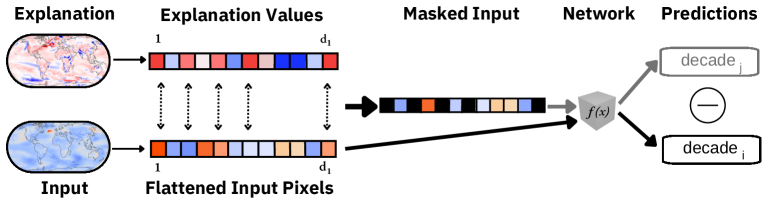
Figure 3: Diagram of the concept behind the faithfulness property. Faithfulness assesses the impact of highly relevant pixels in the explanation map on the network decision. First, the explanation values are sorted to identify the highest relevance values (here shown in red). Next, the corresponding pixel positions in the flattened input temperature map are identified (see dotted arrows) and masked (marked in black); that is, their value is ignored in the input map. Both the masked and the original input maps are passed through the network and their predictions are compared. If the masking is based on a faithful explanation, the prediction of the masked input ($j$, grey) is expected to change compared to (indicated by minus sign) that of the unmasked input ($i$, black), i.e., a different decade is predicted.

To measure this property, we apply Remove and Debias (ROAD) (Rong et al., 2022a) which returns a curve of scores $\hat{\textbf{q}}=:(\hat{q}_{1},\dots,\hat{q}_{I})$ for a chosen percentage range p. Each curve value $\hat{q}_{i}$ corresponds to the average score that is calculated by perturbing a percentage $p_{i}\in\textbf{p}$ of the highest relevant pixel established from the explanation $\Phi^{m}\left(f,c_{n},\mathbf{x}_{n}\right)$ in the input $\mathbf{x}_{n}$. For each input $\mathbf{x}_{n}$ with corresponding perturbed input $\hat{\mathbf{x}}_{n}^{i}$, the ROAD score $\hat{q}^{m}_{ROAD,\,i}$ is calculated as follows:

$$\hat{q}^{m}_{ROAD,\,i}=\frac{1}{N}\sum_{n=1}^{N}\mathbf{1}_{c_{n}}(c_{pred,n})\quad\text{with}\quad\mathbf{1}_{c_{n}}(c_{pred,n})=\begin{cases}1&c_{n}=c_{pred,n}\\ 0&\text{otherwise}\end{cases}$$ (5)

where $\mathbf{1}_{c_{n}}:\mathbf{C}\rightarrow[0,1]$ is an indicator function comparing, the predicted class $c_{pred,n}=f(\hat{\mathbf{x}}_{n}^{i})$ of $\hat{\mathbf{x}}_{n}^{i}$ to $c_{n}=f(\mathbf{x}_{n})$ the predicted class of the unperturbed input $\mathbf{x}_{n}$. We calculate the score values for up to 50 $\%$ of pixel replacements $\mathbf{p}$ of the highest relevant pixel, calculated in steps of $1\%$; resulting in a curve $\hat{\mathbf{q}}^{m}_{ROAD}$. For faithful explanations, this curve is expected to degrade faster towards increasing percentages of perturbed pixels (see Section 3, Eq. (6)). The area under the curve (AUC) is then used as the final ROAD score ${q}^{m}_{ROAD}$:

$${q}^{m}_{ROAD}=\text{AUC}(\mathbf{p},\hat{\mathbf{q}}^{m}_{ROAD})$$ (6)

Accordingly, a lower score corresponds to higher faithfulness and the normalization of the ROAD score also follows Eq. (4).
Furthermore, to measure faithfulness, we consider the faithfulness correlation (FC), defined as:

$$q^{m}_{FC}=\underset{S\in|S|\subseteq d}{\operatorname{corr}}\left(\sum_{i\in S}{\Phi}^{m}(f,c,\mathbf{x})_{i},{f}(\mathbf{x})-{f}\left(\mathbf{x}_{\left[\mathbf{x}_{s}=\overline{\mathbf{x}}_{s}\right]}\right)\right)$$ (7)

where $|S|\subseteq d$ is a subset of random indices of sample $\mathbf{x}$ and a chosen baseline value $\overline{\mathbf{x}}$ (Bhatt et al., 2020). Unlike ROAD, the faithfulness correlation score $\bar{q}^{m}_{\text{FC}}$ increases as the performance improves, which is why we normalize the score as follows:

$$\bar{q}^{m}_{\text{FC}}=\frac{q^{m}_{\text{FC}}}{q^{\text{max}}_{\text{FC}}}$$ (8)

with $q^{\text{max}}_{\text{FC}}=\text{max}\left(q^{m}_{\text{FC}}|q^{m}_{\text{FC}}\in R,\forall m=[1,M]\right)$ defining the maximum across the scores of $M$ explanation methods.

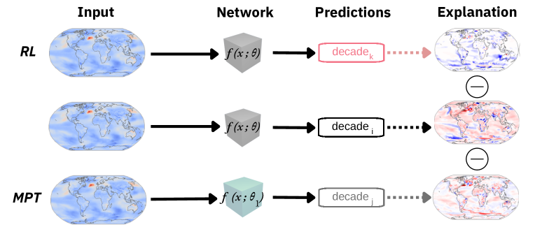
Figure 4: Diagram of the concept behind the randomization property. In the middle row, the original input temperature map is passed through the network, and the explanation map is calculated based on the predicted (grey background) decade. For the random logit (RL) metric (first row), the input temperature map and the network remain unchanged but the decade $k$ used to calculate the explanation is randomly chosen (pink font). The resulting explanation map is then compared to the original explanation (indicated by minus sign) to test its dependence on the class. For the model parameter test (MPT, bottom row), the network is perturbed (see green box) with noisy parameters ($\theta_{1}=\theta+\text{noise}$), potentially altering the predicted decade ($j$, grey). The explanation map of the perturbed model should differ from the original explanation map if the explanation is sensitive to the model parameters.

3.3 Randomisation

This property assesses the effect on the explanation to a random perturbation scenario (See Figure 4). Either the network weights (Adebayo et al., 2018) are randomised or a random class that was not predicted by the network for the input sample $\mathbf{x}$ is explained (Sixt et al., 2020). In both cases, a change in the explanation is expected, since the explanation of an input $\mathbf{x}$ should change if the model changes or if a different class is explained. Here we evaluate randomization based on the model parameter test (MPT) score (Adebayo et al., 2018) and the random logit (RL) score (Sixt et al., 2020). The MPT score is defined as the average correlation coefficient between the explanation of the original model $f$ and the randomized model $f_{\mathbf{W}}$ over all layers $L$:

$$q^{m}_{MPT}=\frac{1}{L}\sum_{i=1}^{L}\rho(\Phi^{m}(f,c,\mathbf{x}),\Phi^{m}(f_{l},c,\mathbf{x}))$$ (9)

where $\rho$ denotes the Spearman rank correlation coefficient and $f_{l}$ is the true model with additive perturbed weights of layer $l$.
The RL score (Sixt et al., 2020) is defined as the structural similarity index ($SSIM$) between heatmaps resulting from explaining a class $\hat{c}$ that was not predicted (with $f(\mathbf{x})=c$, $\hat{c}\neq c$) and heatmaps explaining the predicted label $c$:

$$q^{m}_{RL}=\text{SSIM}(\Phi^{m}(f,c,\mathbf{x}),\Phi^{m}(f,\hat{c},\mathbf{x}))$$ (10)

The metric scores of randomization and the robustness metric behave the same, in that low metric scores indicate strong performance. Thus, the normalization follows Eq. (4).

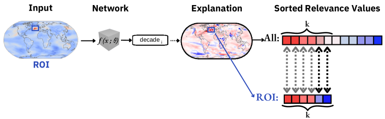
Figure 5: Diagram of the concept behind the localization property. First, an expected region of high relevance for the network decision, the region of interest (ROI), is defined in the input temperature map (blue box). Here, the North Atlantic is chosen, as this region has been discussed to affect the prediction (see Labe and Barnes (2021)). Next, the sorted explanation values of the ROI, encompassing $k$ pixels, are compared to the $k$ highest values of the sorted explanation values across all pixels. An explanation method with strong localization should assign the highest relevance values to the ROI.

3.4 Localisation

The quality of an explanation is measured based on its agreement with a user-defined region of interest (ROI, see Figure 5). This means that the localization of the highest relevant pixels (given by the XAI explanation) should agree with the given labeled areas, e.g. bounding boxes or segmentation masks. Localisation metrics assume that the ROI should be mainly responsible for the network decision (Zhang et al., 2018; Arras et al., 2022; Theiner et al., 2022; Arias-Duart et al., 2022), and an XAI method should, thus, assign high relevance values in the ROI.

As localization metrics here we use the top-$k$-pixel (Theiner et al., 2022) and the relevance-rank-accuracy (RRA) (Arras et al., 2022) which are computed as follows:

$$q^{m}_{TopK}=\frac{\mid{\Phi_{K}^{m}}\cap\mathbf{s}\mid}{\mid K\mid}$$ (11)

$$q^{m}_{RRA}=\frac{\mid{\Phi_{\mathbf{s}}^{m}}\cap\mathbf{s}\mid}{\mid\mathbf{s}\mid},$$ (12)

where $\Phi_{K}^{m}=:\mathbf{r}_{1-K}$ denotes the subset of indices of explanation $\Phi$ that corresponds to the $K$ highest ranked feature, $\mathbf{r}=Rank\left(\Phi^{m}(f,c,\mathbf{x})\right)$ denotes the subset of indices of explanation $\Phi$ that corresponds to the $K$ highest ranked features, and $\mathbf{s}$ refers to the indices of ROI. The corresponding scores are high for well-performing methods and low for explanations with low localization. Accordingly, the score normalization follows Eq. (8).

Figure 6: Diagram of the concept behind the complexity property. Complexity assesses how the evidence values are distributed across the explanation map. For this, the distribution of the relevances from the original explanation are compared to that of a “random” explanation drawn from a random uniform distribution. Here, shown in a 1-D example, the evidence distribution of the explanation exhibits clear maxima and minima (see maxima in red oval), which is considered desirable and linked to increased scores. The noisy features show a uniform distribution linked to a low complexity score.

3.5 Complexity

Complexity is a measure of conciseness, meaning that an explanation should consist of a few strong features (Chalasani et al., 2020; Bhatt et al., 2020) (See Figure 6). The assumption behind this is that concise explanations with strong features are easier for the researcher to interpret and include a higher information content with less noise.

Here, we use complexity (Bhatt et al., 2020) and sparseness as representative metric functions (Chalasani et al., 2020), which are formulated as follows:

$$q_{COM}=\mathbb{P}_{\Phi}(i)=\frac{\left|{\Phi}({f},c,\mathbf{x})_{i}\right|}{\sum_{j\in[d]}\left|{\Phi}({f},c,\mathbf{x})_{j}\right|};\mathbb{P}_{{\Phi}}=\left\{\mathbb{P}_{{\Phi}}(1),\ldots,\mathbb{P}_{{\Phi}}(d)\right\},$$ (13)

$$q_{SPA}=\frac{\sum_{i=1}^{d}(2i-d-1)\Phi(f,\mathbf{x})}{d\sum_{i=1}^{d}\Phi(f,\mathbf{x})},$$ (14)

where $\mathbb{P}_{\Phi}$ is a valid probability distribution; $\mathbb{P}_{{\Phi}}(i)$ denotes the fractional contribution of the feature $\mathbf{x}_{i}$ to the total magnitude of the attribution. Sparseness is based on the Gini index (Hurley and Rickard, 2009), Complexity is calculated as the entropy. Since low entropy is desirable, the score is normalized based on Eq. (4). For Eq. (14), a high Gini index indicates sparseness, and the score is normalized based on Eq. (8).

Experiments

4.1 Network predictions, explanations and motivating example

We evaluate the network performance and discuss the application of the explanation methods for both network architectures. Aside from the learning rate $l$ with ($l_{\text{CNN}}=0.001$), we maintain comparability to Labe and Barnes (2021) by fixing a similar set of the hyperparameters and the fuzzy classification setup for the MLP and the CNN during training. Here we use the regression part of the fuzzy classification only as a performance measure (see Appendix B.1). Following the training and testing (Section 2.2), both the MLP and the CNN have a similar performance compared to the primary publication (Figure 3c in Labe and Barnes (2021)). While the CNN slightly outperforms the MLP in terms of $RMSE$ (see Figure 9), the classification accuracy of both networks agrees within error bounds (see Appendix B.1 for detailed performance discussion). This ensures that evaluation score differences between the MLP and the CNN are not caused by differences in network accuracy.

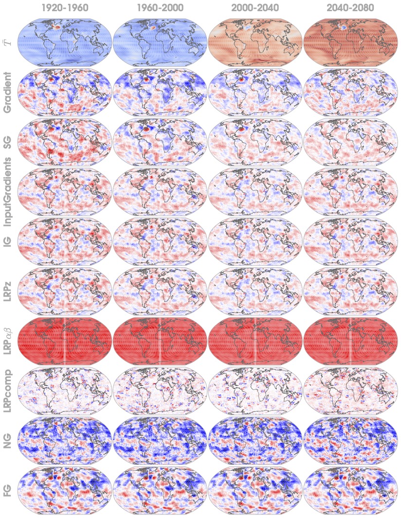
Figure 11: CNN explanation map average over $1920-1960$,$1960-2000$, $2000-2040$ and $2040-2080$ for all XAI methods. The first row shows the average input temperature map $\bar{T}$ with the colorbar ranging from maximum (red) to minimum(blue) temperature anomalie. All consecutive lines show the explanation maps of the different XAI methods with colorbar ranging from $1$ (red) to $-1$ (blue).

We calculate the explanation maps for all temperature maps, that were correctly predicted (see Appendix B.1 for details). All XAI methods presented in Section 2.3 are applied to explain the predictions of both MLP and CNN. Note that the composite rule of LRP converges to the LRP-$z$ rule for the MLP model due to its dense layer architecture (Montavon et al., 2019). For NoiseGrad, SmoothGrad and FusionGrad, we use the Gradient method as the baseline explanation method. Explanation maps of all XAI methods and for both networks are shown exemplary for the year $2035$ in Figures 10 and 11.

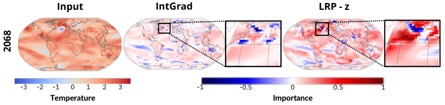
Figure 7: Motivating example visualizing the difference between different XAI methods. Shown are the T2m-temperature map for the year $2068$ with the corresponding IntGrad and LRP-$z$ explanation maps of the MLP. For both XAI methods, red means that pixels contribute positively and blue means that corresponding pixels contribute negatively to the predicted class. Next to the explanation maps, a zoomed-in map of the North Atlantic region (NA, $10-80^{\circ}$W, $20-60^{\circ}$N) is shown, indicating partly different evidences of Integrated Gradients and LRP-$z$.

To motivate the application of XAI evaluation, we show that different XAI methods can provide different relevances. Labe and Barnes (2021) showed that the cooling patch in the North Atlantic (NA) contributes to the network prediction. However, each XAI method assigns different contributions to this region (see also Appendix B.2). Figure 7 exemplifies this showing the temperature map of the year $2068$ alongside the explanation maps of LRP-$z$ and Integrated Gradients. Zoomed-in map sections only $58-70^{\circ}$W, $34-44^{\circ}$N for each XAI method.

In the Integrated Gradients explanation, the relevance assigned to the NA does not stand out compared to other regions, e.g. Australia. In contrast, in the LRP-$z$ explanation, the NA patch contributes strongly to the network decision with high relevances. Furthermore, for Integrated Gradients the NA region shows overall weak positive and stronger negative contributions, while in the LRP-$z$ explanation, it contributes largely positively, except for the ocean area between Canada and Greenland. Thus, in contrast to Integrated Gradients, the LRP-$z$ explanation suggests that the cooling patch in the NA is important positive predictors for the decade $2060-2069$. In other words, different explanations can lead to different scientific conclusions and this compounds the choice of an explanation method.

4.2 Assessment of XAI Metrics

We evaluate the different XAI evaluation properties for the classification task (see Section 2.2) on the MLP and address challenges of its application in climate science, such as data with large internal variability and the requirement of physically informed networks. We analyze two representative metrics for each property and base our analysis on three criteria: the coherence of the XAI evaluation metric score between metrics within one property, the score stability across multiple metric runs, and the information value carried by the scores, which coincides with previous research (Mamalakis et al., 2021, 2022). Additionally, we provide an artificial random explanation baseline for each metric as a simple benchmarking procedure (Rieger and Hansen, 2020). This baseline helps determine whether a metric can distinguish between a simple uniform random image and an explanation. Details on the baseline and our criteria can be found in Appendix A.2.

Table 1 displays the results of the robustness metrics, including the mean score and the standard error of the mean (SEM) across the evaluation scores of $50$ explanation samples (as defined in Equation 26). In order to make the AS and LLE scores comparable, we draw $10$ perturbed samples per temperature map, as described in Section 3. More details about the hyperparameters used for the metrics are provided in Appendix B.2.

Table 1: Performance assessment of different robustness and faithfulness metrics compared to a uniform random baseline explanation (highlighted in grey). The highest scores are bold and correspond to the best performance for the given metric. The lowest scores are red. We report the mean and SEM of all scores (see Eq. (26)).

	Robustness		Faithfulness
XAI	Average Sensitivity	Local Lipschitz Estimate	ROAD	Faithfulness Correlation
Random Baseline	0.052 $\pm$ 0.006	0.035$\pm$ 0.005	0.58 $\pm$ 0.04	0.14 $\pm$ 0.02
FusionGrad	0.09$\pm$ 0.01	0.059 $\pm$ 0.009	0.61 $\pm$ 0.04	0.35 $\pm$ 0.04
InputGradients	0.47 $\pm$ 0.03	0.57 $\pm$ 0.04	0.99 $\pm$ 0.02	0.87 $\pm$ 0.03
LRP-$z$	0.47 $\pm$ 0.04	0.57 $\pm$ 0.04	0.99 $\pm$ 0.02	0.85 $\pm$ 0.03
Integrated Gradients	0.56 $\pm$ 0.04	0.58 $\pm$ 0.04	1.000 $\pm$ 0.02	0.86 $\pm$ 0.03
SmoothGrad	0.51 $\pm$ 0.04	0.43 $\pm$ 0.05	0.65 $\pm$ 0.04	0.67 $\pm$ 0.03
LRP-$\alpha$-$\beta$	0.91 $\pm$ 0.03	0.88 $\pm$ 0.03	0.91 $\pm$ 0.02	0.36 $\pm$ 0.03
Gradient	0.50 $\pm$0.04	0.45 $\pm$ 0.05	0.66 $\pm$ 0.04	0.77 $\pm$ 0.04
NoiseGrad	0.09 $\pm$ 0.01	0.06 $\pm$ 0.01	0.61 $\pm$ 0.03	0.51 $\pm$ 0.03

The robustness metrics both pass the random baseline test, with the lowest score corresponding to the random baseline and significant differences to the other scores. LRP-$\alpha$-$\beta$ has the highest robustness scores with mean values as high as $0.91$, while FusionGrad and NoiseGrad have the lowest robustness across all methods, with scores below $0.1$. The remaining XAI methods show normalized scores around $0.5$. We attribute these results to the large internal variability inherent in the climate input data, leading to increased uncertainty in the network predictions. In other words, learning from noisy data results in noisy decisions (Sonnewald and Lguensat, 2021; Clare et al., 2022). As a consequence, additional data and network perturbations have a greater impact on the prediction behavior, and subsequently on the explanations of the inherently noisy climate data. XAI methods with perturbation averaging (such as NoiseGrad and FusionGrad) are more susceptible to data perturbations and are therefore less robust. In contrast, explanation methods with limited feature content, such as LRP-$\alpha$-$\beta$ considering only features with positive contribution, also consider fewer variations, are less susceptible to input perturbations, and indicate higher robustness.
However, except for the three lowest (including random baseline) and the highest score, AS and LLE scores do not align. All other AS within the SEM, whereas only the LLE scores of theoretically similar explanation methods overlap, such as InputGradients, LRP-$z$, and Integrated Gradients (see Section 2.3) (Mamalakis et al., 2022). The difference in score distribution between LLE and AS can be associated with the various similarity functions used to calculate the scores (see Section 3) with the LLE score weighting the explanation distance by the input distance. The LLE score accounts for the internal variability of the data, resulting in scores that are in line with theoretical expectations.

The results of the faithfulness metrics, FC and ROAD, are presented in Table LABEL:tab:RFRmetrics, with the hyperparameters discussed in Appendix B.2. Although FC passes the random baseline test, the ROAD scores of NoiseGrad and FusionGrad overlap with the random baseline score within the SEM. For both metrics, InputGradients, Integrated Gradients and LRP-$z$ have the highest scores, suggesting that explanation methods considering input contributions provide more meaningful relevance values. Other explanation method scores, as well as the random baseline, differ in magnitude between metrics. LRP-$\alpha$-$\beta$ exhibits a mean score of $0.91$ for ROAD and only $0.36$ for FC, which we attribute to different calculation procedures. The ROAD method perturbs an increasing percentage of highly relevant pixels leading to higher scores for explanations considering only positive contributions, whereas FC perturbs random pixels.
All ROAD scores are grouped into two groups of overlapping scores, except for LRP-$\alpha$-$\beta$ as the outlier. From the LRP-$\alpha$-$\beta$ score, we conclude that negative evidence also carries information that impacts the network decision. The low score and respective similarity to the random baseline of gradient-based explanations are potentially due to increased network uncertainty, leading to more noise in gradients, thus displaying less faithful evidence.
For FC scores, similar conclusions can be drawn. Gradient-based methods exhibit decreased faithfulness. Additionally, we find that input or network perturbations, such as SmoothGrad and NoiseGrad, decrease faithfulness further, with the strongest decrease for both types of perturbations as in FusionGrad. These results again indicate increased network uncertainty but can also be attributed to higher input similarity between classes (similar temperature maps for successive years), with proposed noise smoothing procedures causing a loss of class-defining evidence.

Table 2: Performance assessment of randomization, complexity and localization metrics based on a comparison to a uniform random baseline (highlighted in grey). The highest scores are printed in bold and correspond to the best performance for the given metric. All scores are reported based on mean and standard error of the mean, defined in Eq. (26) and (27).

	Randomisation		Complexity		Localisation
XAI	MPT	Random Logit	Complexity	Sparseness	TopK	RRA
Random Baseline	0.0027 $\pm$ 0.0002	0.0026 $\pm$ 0.0003	0.914 $\pm$ 0.003	0.492 $\pm$ 0.006	0.18 $\pm$ 0.02	0.19 $\pm$0.02
FusionGrad	0.40 $\pm$ 0.03	0.86 $\pm$ 0.04	0.946 $\pm$ 0.003	0.770 $\pm$ 0.006	0.65 $\pm$ 0.04	0.87 $\pm$ 0.04
InputGradients	0.0096 $\pm$ 0.0008	0.018 $\pm$ 0.003	0.988 $\pm$ 0.002	0.968 $\pm$ 0.004	0.63 $\pm$ 0.05	0.53 $\pm$ 0.04
Integrated Gradients	0.0091 $\pm$ 0.0007	0.04 $\pm$ 0.02	0.986 $\pm$ 0.002	0.950 $\pm$ 0.003	0.62 $\pm$ 0.05	0.59 $\pm$ 0.04
LRP-$z$	0.0096 $\pm$ 0.0008	0.018 $\pm$ 0.003	0.988 $\pm$ 0.002	0.968 $\pm$ 0.004	0.63 $\pm$ 0.05	0.52 $\pm$ 0.04
SmoothGrad	0.52 $\pm$ 0.03	0.014 $\pm$ 0.002	0.943 $\pm$ 0.003	0.749 $\pm$ 0.006	0.42 $\pm$ 0.03	0.50 $\pm$ 0.04
LRP-$\alpha$-$\beta$	0.0071 $\pm$ 0.0005	0.0028 $\pm$ 0.0004	0.993 $\pm$ 0.002	0.95 $\pm$ 0.01	0.65 $\pm$ 0.06	0.61 $\pm$ 0.05
NoiseGrad	0.60 $\pm$ 0.03	0.38 $\pm$ 0.05	0.953 $\pm$ 0.003	0.821 $\pm$ 0.006	0.36 $\pm$ 0.04	0.47 $\pm$ 0.03
Gradient	0.53 $\pm$ 0.03	0.022 $\pm$ 0.005	0.944 $\pm$ 0.003	0.768 $\pm$ 0.007	0.48 $\pm$ 0.04	0.53 $\pm$ 0.04

Table 2 displays the mean and SEM scores of the randomization metrics, MPT and RL, with their hyperparameters listed in Appendix B.2. The random baseline results have the lowest scores for both metrics, but only the MPT score is significantly different from the low LRP-$\alpha$-$\beta$ score of $0.0071\pm 0.0005$. The highest scores are found for NoiseGrad (MPT) and FusionGrad (RL).
The RL scores of all explanation methods, except for the highest FusionGrad (highest), and NoiseGrad overlap (mean scores overlap within one SEM magnitude). For example, Integrated Gradients overlaps with Gradient, LRP-$z$, and InputGradients. We interpret the similar RL scores as a result of the network task, which requires a definition of classes based on decades with an underlying continuous temperature trend. This means that differences in the temperature maps can be small for subsequent years, and the network decision and explanation for different classes can include similar features. As the RL metric requires a high explanation difference for different classes, close temperature map resemblance would lead to a decreasing score. Similar reasoning applies to the low RL scores of the explanation methods that consider input contribution, such as LRP-$z$, InputGradients, IntGrad, and LRP-$\alpha$-$\beta$, which multiply by the input and further enhance explanation similarity.
In contrast, methods with network perturbation (Bykov et al., 2021), such as NoiseGrad and FusionGrad, smooth the decision boundaries and enhance the class differences, corresponding to stronger explanation differences and, subsequently, higher scores. Our findings suggest that caution is needed in using RL, whereas the MPT metric is more advantageous to evaluate explanations on classification tasks involving classes that are not well separable from each other, such as decades on a continuous temperature trend.

We present the complexity evaluation results in Table 2. Both Complexity and Sparseness metrics’ hyperparameters are based on the literature (Chalasani et al., 2020; Bhatt et al., 2020). The random baseline receives the lowest score from both metrics. LRP-$\alpha-\beta$ scores highest in complexity, while InputGradients and LRP-$z$ receive the highest sparseness scores. Nevertheless, both metrics provide similar insights. SmoothGrad, Gradient, and FusionGrad are the three least-sparse methods, with NoiseGrad following. The results for NoiseGrad, SmoothGrad, and FusionGrad can be attributed to the smoothing effect caused by averaging several explanations. LRP-$z$, InputGradients, Integrated Gradients, and LRP-$\alpha$-$\beta$ receive higher scores as they consider input contributions. Complexity scores are high ($>0.91$) and closely distributed (largest difference of $<0.08$), while sparseness scores deviate more from the random baseline score (lowest score deviates by $\sim 50\%$). The Gini index and Shannon entropy measures are used for Sparseness and Complexity metrics, respectively (see Eq. (14) and (13)). Climate data exhibits high internal variability, leading to noisier explanations, closer to the uniform random baseline in entropy. The Gini index is less susceptible to the high noise of climate data, deviating between a flat explanation (lowest score) and an explanation with few groups of highly relevant pixels (highest score). Hence, the sparseness metric might be the more compatible choice to evaluate the explanation complexity in the climate context.

Lastly, we present results of the localization metrics (left-most columns of Table 2). Based on Labe and Barnes (2021), we choose the NA region ($58-70^{\circ}$W, $34-44^{\circ}$N) as our region of interest (ROI), as the cooling patch in this region is a known feature of climate change (Labe and Barnes, 2021). We calculate the Top-$k$ scores for $k=10\%$ of the pixels in the image and maintain all other hyperparameters according to literature settings (Arras et al., 2022). Both the Top-$k$ and the RRA metrics pass the random baseline test, which is expected as the random uniform explanation, by construction, has no minima and maxima in the ROI (see Figure 5). For RRA, FusionGrad corresponds to the highest score. All other explanation methods exhibit lower but similar localization scores, which suggests that the ROI is captured equally in all explanations. Due to the overall high and strongly overlapping scores, we cannot infer characteristic information about the explanation methods. These results suggest that the strength of localization metrics lies in probing the network decision with respect to learning established physical phenomena rather than XAI performance assessment.

4.3 Network-based comparison

To compare the performance of explanation methods for the MLP and CNN network, we selected one metric per property based on our previous results, LLE (robustness), FC (faithfulness), Randomization, Sparseness (complexity) and RRA (localization). Although, defining a meaningful ROI for localization and defining localization as a explanation property presents challenges (see Section 4.2), we included RRA localization metric for the purpose of a complete evaluation.
Table 3 displays the results for both networks across all properties, reporting the rank (from highest to lowest score) of the XAI methods, as is commonly done for explanation comparison (Hedström et al., 2023; Tomsett et al., 2022; Rong et al., 2022b; Brocki and Chung, 2022; Gevaert et al., 2022). If differences in the mean scores were within the range of the SEM, the same rank was assigned. The CNN and MLP have similarities in ranking across every category, but differences are sightly stronger for localization and complexity due to structural differences in learned patterns. In other words, the CNN exhibits more clustered evidence compared to the MLP (see Figure 11 and 10) leading to ranking differences in properties that assess spatial distribution of evidence in the image.
In general we find that, explanation methods with input contribution, such as Integrated Gradients, InputGradients, and LRP, consistently achieved the best rankings in faithfulness, robustness, and complexity, but were susceptible to the network parameters and decision boundaries, known as randomization. The inverse is true for gradient-based methods, such as Gradient, SmoothGrad, NoiseGrad, and FusionGrad, which achieved the best rankings in randomization and showed lower performance in faithfulness, robustness, and complexity. The low rankings of LRP-$\alpha$-$\beta$ and LRP-composite in the faithfulness category are the only exception to the previous results. Thus, for both networks, we find that neglecting negative evidence, as for LRP-$\alpha$-$\beta$, results in the less faithful explanation. While LRP-composite outperforms the $\alpha$-$\beta$-rule, the method may neglect faithful evidence to form less-complex explanations.

	Robustness		Faithfulness		Randomisation		Complexity		Localisation
	MLP	CNN	MLP	CNN	MLP	CNN	MLP	CNN	MLP	CNN
FusionGrad	4.	5.	5.	5.	3.	1.	4.	3.	1.	1.
InputGradients	2.	3.	1.	1.	4.	4.	1.	2.	2.	4.
Integrated Gradients	2.	3.	1.	1.	4.	4.	2.	2.	2.	2.
LRP-$z$	2.	3.	1.	1.	4.	4.	1.	2.	2.	4.
SmoothGrad	3.	3.	3.	3.	2.	2.	5.	3.	2.	2.
LRP-$\alpha$-$\beta$	1.	2.	5.	7.	5.	5.	2.	4.	2.	3.
NoiseGrad	4.	4.	4.	4.	1.	2.	3.	3.	2.	5.
Gradient	3.	3.	2.	2.	2.	3.	4.	3.	2.	4.
LRP-composite	$-$	1.	$-$	6.	$-$	4.	$-$	1.	$-$	6.

Table 3: Comparison of CNN and MLP results of the explanation method ranking in the different evaluation categories from best (rank one in bold) to worst (in italics). We do not report results for the LRP-composite explanations of the MLP as the method targets CNNs specifically. We base the ranking on the results of the mean scores across $N=50$ explanations; the same ranks correspond to a score agreement within the SEM.

For explanation-enhancing procedures such as SmoothGrad, Integrated Gradients, FusionGrad and NoiseGrad (see Section 2.3) both CNN and MLP results indicate no improvement of the explanation performance. Contrary to theoretical assumptions (see Appendix A.1), we find consistent or decreasing ranks of these XAI methods compared to the explanation method which is used as a baseline for enhancements, such as InputGradients for Integrated Gradients or Gradient for SmoothGrad, NoiseGrad and FusionGrad, except for randomization (see SmoothGrad, NoiseGrad and FusionGrad) and complexity for NoiseGrad. We attribute the decrease in ranking to the internal variability in the climate data and the successively high network uncertainty. The different input and network perturbation techniques used to enhance SmoothGrad, Integrated Gradients, NoiseGrad and FusionGrad (see Section 2.3) add additional uncertainty, possibly leading to shifts in the class prediction of the perturbed temperature map. Thus, the average across the perturbed input explanations might average out important evidence for the true class.

4.4 Choosing a XAI method

As XAI evaluation allows a comparison of the performance of explanation methods, we propose to use it to select an appropriate XAI method. As a first step, practitioners should determine which explanation properties are essential for their specific network task, which may well vary depending on context. For instance, for physically informed networks, randomization might be a crucial property, since network parameters carry physical meaning and their successive randomization should lead to a significant change in the network’s performance (see Section 3). Localisation, on the other hand, might be neglected if a region of interest cannot be determined a priori. Once these essential properties are identified, practitioners can apply accessible XAI methods and calculate the normalized evaluation scores in each chosen property. This allows a ranking of explanation methods to determine the optimal XAI method for the given task.

For our specific task, we aim for an explanation that is robust towards variation across the simulated ensemble members (see Section 2.1), displays significant features (complexity) without sacrificing faithful evidence, and captures the network parameter behavior (randomization). As enabled in the Quantus XAI evaluation library (Hedström et al., 2023), we visualize the score performance for the MLP (see Table 1 and 2) in a spyder plot (Figure 8), with the outermost lines refer to the best performing XAI method for a given property. According to the properties we want to be fulfilled, LRP-$z$ (cyan) and InputGradients (green, aligned with the cyan pentagon) provide the most reliable explanations (according to Table 3 and Figure 8), followed by Integrated Gradients (red). The results further indicate that the randomization performance can be improved by considering NoiseGrad (brown), with only a minor decrease (one rank) in robustness and faithfulness performance (see rank difference between Gradient and NoiseGrad in Table 3).

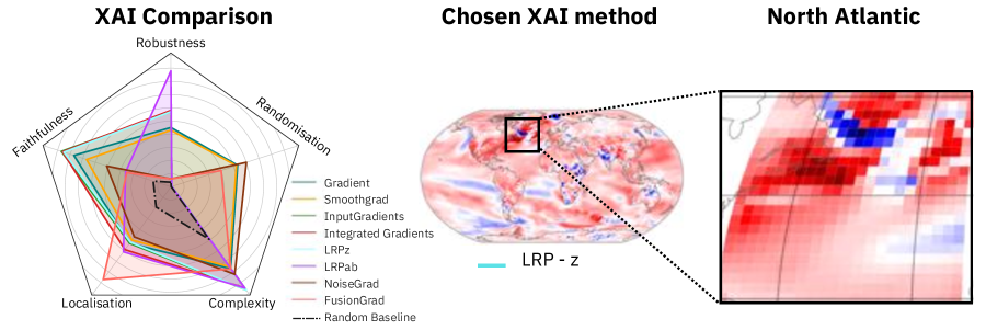
Figure 8: Visualization of the proposed procedure to choose an appropriate XAI method. In the spyder plot (left) the scores in all properties across nine explanation methods applied to the MLP are visualized, according to Table 3. The spyder plot can be used as a visual aid alongside the ranks in each essential category to determine the best-performing XAI method. In the plot the best rank corresponds to the furthest distance from the center of the graph. Thus, ideally an explanation method with outermost lines in all categories corresponds to the best performance across all properties. Based on both the Table 3 and the spyder plot LRP-$z$ and InputGradients are equally appropriate choices. In the middle, the LRP-$z$ explanation map of the decade prediction on the temperature map of $2068$, is shown. The established best-performing method to verify the findings on the impact of the NA region (right) discussed in Section 4.1.

Based on our evaluation, we would select LRP-$z$ to explain the MLP predictions and use the gained insight to interpret the explanations in Figure 7, which relates to the analysis of the impact of the NA region (see Section 4.1). From the explanation, we can see that the network heavily depends on the NA region and is capable of recognizing the cooling patch pattern, enabling it to accurately identify the correct decade in this simulation scenario of global warming.

Discussion and Conclusion

XAI methods aim to improve the understanding of the complex relationships learned by DNNs and can provide novel insights into climate AI research (Camps-Valls et al., 2020; Gibson et al., 2021; Dikshit and Pradhan, 2021; Mayer and Barnes, 2021; Labe and Barnes, 2021; van Straaten et al., 2022; Labe and Barnes, 2022). However, the increasing number of available XAI methods raises two questions: Which explanation method is trustworthy, and which is an appropriate choice for a given task? (Leavitt and Morcos, 2020; Mamalakis et al., 2021, 2022). This issue is illustrated in our motivating example (Figure 7).
To address these questions, we introduced XAI evaluation to climate science. Building upon existing research (Labe and Barnes, 2021) we evaluate various local, model-aware explanation methods. These methods are applied to an MLP and a CNN which assign yearly temperature maps to the corresponding decade class. Given comparable network performances, we then evaluate the XAI methods on the basis of five different properties, namely, robustness, faithfulness, randomization complexity and localization, providing quantitative measures for the quality of an explanation method. For each property, two metrics are explored and compared to a random baseline test on the MLP task (Alvarez-Melis and Jaakkola, 2018; Montavon et al., 2019; Yeh et al., 2019; Bhatt et al., 2020; Arras et al., 2022; Rong et al., 2022a; Hedström et al., 2023). Lastly, based on the metric assessment results, we perform the evaluation across all properties and XAI methods and compare the results between MLP and CNN.

Our results demonstrate that the different metrics vary in their compatibility with climate data. The robustness metric LLE accounts better than AS for its internal variability. In the randomization assessment, we find that the MPT metric is favorable for classification tasks defined on continuous data, whereas regarding the explanation complexity, the Sparseness metric is more suitable for data with natural variability. Lastly, the baseline test in Localization suggests that, in the climate context, localization can be used to identify if the ROI was learned by the network. Although our experiments showcase XAI evaluation for a single climate task, the evaluated properties are also applicable to other research questions. For example, from the robustness scores of the explanations, we learn that the scoring is affected by the increased data and network noise (Clare et al., 2022).

Comparing the explanation performance between MLP and CNN, we can state that in general our findings are consistent with prior research (Mamalakis et al., 2021, 2022). The results indicate that explanation methods considering input contributions perform better in terms of faithfulness, complexity, and robustness independent of the considered network structure. However, we also find LRP-$\alpha$-$\beta$ and LRP-$composite$ to be exceptions, which by neglecting negative evidence and reducing complexity respectively, result in the least faithful explanation. Moreover, we find that gradient-based methods capture the network parameter influence more reliably, corresponding to higher randomization scores. Except for randomization, explanations using averages across perturbations, such as SmoothGrad, NoiseGrad, FusionGrad and Integrated Gradients, do not increase the robustness, faithfulness and complexity, contrary to theoretical motivations and previous claims.

To choose the optimal explanation method for a specific research task, we propose an XAI evaluation guideline. By, firstly, identifying the XAI properties which are important for network and data, the evaluation is targeted to the research question at hand. Secondly, the normalized evaluation scores across the properties are calculated for different XAI methods. To compare the methods, the scores are ranked and the researcher can determine the highest-ranking XAI method. For our classification task, for example, we find LRP-$z$ and InputGradients to be the best-performing methods in the MLP task and LRP-$z$, InputGradients and Integrated Gradients in the CNN task. Returning to our motivating example (Figure 7), we demonstrate based on the NA region that XAI evaluation subsequently facilitates a more trustworthy interpretation of the explained evidence.

With this work, we demonstrate the potential of XAI evaluation for climate AI research. XAI evaluation offers thorough and novel information about the structural properties of explanation methods, providing a more specific comparison and evaluation of explanation performance, thereby supporting researchers in the choice of an appropriate explanation method, independent of the network structure.

Acknowledgments

This work was funded by the German Ministry for Education and Research through project Explaining 4.0 (ref. 01IS200551). The authors also acknowledge the CESM Large Ensemble Community Project (Kay et al., 2015) for making the data publicly available.

Datastatement

Our study is based on the RPC8.5 configuration of the CESM1 Large Ensemble simulations (data instructions). The data is freely available (https://www.cesm.ucar.edu/projects/community-projects/LENS/data-sets.html). The source code for all experiments is accessible at (Github Source Code). All experiments and code are based on Python v3.7.6, Numpy v1.19 (Harris et al., 2020), SciPy v1.4.1 (Virtanen et al., 2020), Matplotlib v3.2.2 (Caswell et al., 2020), and colormaps provided by Matplotlib v3.2.2 (Caswell et al., 2020). Additional Python packages used for development of the ANN, explanation methods and evaluation include Keras/TensorFlow (Abadi et al., 2016), iNNvestigate (Alber et al., 2019) and Quantus (Hedström et al., 2023). We implemented all explanation methods except for NoiseGrad and FusionGrad using iNNvestigate (Alber et al., 2019). For XAI methods by (Bykov et al., 2022) and Quantus (Hedström et al., 2023) we present a Keras/TensorFlow (Abadi et al., 2016) adaptation in our repository. All dataset references are provided throughout the study.

Appendix A Additional Methodology

A.1 Explanations

To provide a theoretical background we provide formulas for the different XAI methods we compare, in the following Section. Gradient
The gradient method is the weak derivative $\nabla_{x}:=\nabla f(\mathbf{x})$ of the network output $f(\mathbf{x})$ with respect to each entry of the temperature map $\mathbf{x}\in\mathbf{x}$ (Baehrens et al., 2010).

$$\Phi(f(\mathbf{x}))=\nabla_{x}$$ (15)

Accordingly, the raw gradient has the same dimensions as the input sample $\nabla_{x},\mathbf{x}\in\mathbb{R}^{D}$.

InputGradient
InputGradient explanations are based on a point-wise multiplication of the impact of each temperature map entry on the network output, i.e. the weak derivative $\nabla_{x}$, with the value of the entry in the explained temperature map $\mathbf{x}$. All explanations are calculated as follows:

$$\Phi(f(\mathbf{x}))=\nabla_{x}\mathbf{x}$$ (16)

with $\Phi(f(\mathbf{x})),\nabla_{x},\mathbf{x}\in\mathbb{R}^{D}$

Integrated Gradients
The Integrated Gradient method aggregates gradients along the straight line path from the baseline $\overline{\mathbf{x}}$ to the input temperature map $\mathbf{x}$. The relevance attribution function is defined as follows:

$$\Phi(f(\mathbf{x}))=(\mathbf{x}-\overline{\mathbf{x}})\odot\int_{0}^{1}\nabla f(\overline{\mathbf{x}}+\alpha(\mathbf{x}-\overline{\mathbf{x}}))\,\text{d}\alpha,$$ (17)

where $\odot$ denotes the element-wise product and $\alpha$ is the step-width from $\overline{\mathbf{x}}$ to $\mathbf{x}$.
Layerwise Relevance Propagation (LRP)
For LRP, the relevances of each neuron $i$ in each layer $l$ are calculated based on the relevances of all connected neurons $j$ in the higher layer $l+1$ (Samek et al., 2017; Montavon et al., 2017).
For the $\alpha$-$\beta$-rule the weighted contribution of a neuron $j$ to a neuron $i$, i.e., $z_{ij}=a_{i}^{(l)}w_{ij}^{(l,l+1)}$ with $a_{i}^{(l)}=x_{i}$, are separated in a positive $z^{+}_{ij}$ and negative $z^{-}_{ij}$ part. Accordingly, the propagation rule is defined by:

$$R_{i}^{(l)}=\sum_{j}\left(\alpha\frac{z^{+}_{ij}}{\sum_{i}z^{+}_{ij}}+\beta\frac{z^{-}_{ij}}{\sum_{i}z^{-}_{ij}}\right)$$ (18)

with $\alpha$ as the positive weight, $\beta$ as negative weight and $\alpha+\beta=1$ to maintain relevance conservation. We set $\alpha=1$ and $\beta=0$
The z-rule accounts for the bounding that input images in image classification are exhibiting, by multiplying positive network weights $w_{ij}^{+}$ with the lowest pixel value $l_{i}$ in the input and the negative weights $w_{ij}^{-}$ by the highest input pixel value $h_{i}$ (Montavon et al., 2017). The relevance are calculated as follows:

$$R_{i}^{(l)}=\sum_{j}\frac{z_{ij}-l_{i}w_{ij}^{+}-h_{i}w_{ij}^{+}}{\sum_{i}z_{ij}-l_{i}w_{ij}^{+}-h_{i}w_{ij}^{+}}$$ (19)

For the composite-rule the relevances of the last layers with high neuron numbers are calculated based on LRP-$0$ (see Bach et al. (2015)), which we drop due to our small network. In the middle layers propagation is based on LRP-$\epsilon$, defined as:

$$R_{i}^{(l)}=\sum_{j}\alpha\frac{a_{j}(w_{ij}+\gamma w_{ij}^{+})}{\sum_{i}a_{j}(w_{ij}+\gamma w_{ij}^{+})}$$ (20)

The relevance of neurons in the layer before the input follows from LRP-$\gamma$

$$R_{i}^{(l)}=\sum_{j}\alpha\frac{z_{ij}}{\sum_{i}z_{ij}}$$ (21)

and the relevance of the input layer is calculated based on equation 19.
SmoothGrad
The SmoothGrad explanations are defined as the average over the explanations of $M$ perturbed input images $\mathbf{x}+\mathbf{g}_{i}$ with $i=[1,\dots,M]$.

$$\Phi(f(\mathbf{x}))=\frac{1}{M+1}\sum_{i=0}^{M}\Phi_{0}(f(\mathbf{x}+\mathbf{g}_{i}))$$ (22)

The additive noise $\mathbf{g}_{i}\sim\mathcal{N}(0,\sigma)$ is generated using a Gaussian distribution.
NoiseGrad
NoiseGrad samples $N$ sets of perturbed network parameters $\hat{\bm{\theta}}_{i}=\bm{\eta}_{i}\bm{\theta}$ using multiplicative noise $\bm{\eta}_{i}\sim\mathcal{N}(\mathbf{1},\bm{\sigma})$. Each set of perturbed parameters $\hat{\bm{\theta}}_{i}$ results in a perturbed network $f_{i}(\mathbf{x}):=f(\mathbf{x};\hat{\bm{\theta}}_{i})$, which are all explained by a baseline explanation method $\Phi_{0}(f(\mathbf{x}))$. The NoiseGrad explanation is calculated as follows:

$$\Phi(f(\mathbf{x}))=\frac{1}{N+1}\sum_{i=0}^{N}\Phi_{0}(f_{i}(\mathbf{x}))$$ (23)

with $f_{0}(\mathbf{x})=f(\mathbf{x})$ being the unperturbed network.
FusionGrad
For FusionGrad the NG procedure is extended by combining the SG procedure using $M$ perturbed input samples with NG calculations. Accordingly, FG can be calculated as follows:

$$\Phi(f(\mathbf{x}))=\frac{1}{M+1}\frac{1}{N+1}\sum_{j=0}^{M}\sum_{i=0}^{N}\Phi_{0}(f_{i}(\mathbf{x}_{j}))$$ (24)

For visualizations, as depicted in Figure 10 and 11 we maintain comparability of the relevance maps $\Phi(f(\mathbf{X}_{i,t}))=\bar{R}^{(i,t)}\in\mathbb{R}^{vxh}$ across different methods, by applying a min-max normalization to all explanations:

$$\bar{R}^{i}=\frac{\mathbb{I}_{\text{max}}R^{i}}{\mathrm{max}\left(r_{jk}|r_{jk}\in R^{i}\forall j\in[1,v]\forall k\in[1,h]\right)}-\frac{\mathbb{I}_{\text{min}}R^{i}}{\mathrm{min}\left(r_{jk}|r_{jk}\in R^{i}\forall j\in[1,v]\forall k\in[1,h]\right)}$$ (25)

with $\mathbb{I}_{\text{min}},\mathbb{I}_{\text{max}}\in\mathbb{R}^{vxh}$ defining corresponding minimum/maximum indicator masks, i.e. for the minimum indicator each entry $\mathrm{\mathbf{i}}_{\text{min}}^{(jk)}=1,\forall r_{jk}<0$ and $\mathrm{\mathbf{i}}_{\text{min}}^{(jk)}=0\forall r_{jk}\geq 0$, for the maximum indicator entries are defined reversely $\mathrm{\mathbf{i}}_{\text{max}}^{(jk)}=1,\forall r_{jk}\geq 0$ and $\mathrm{\mathbf{i}}_{\text{max}}^{(jk)}=0$ otherwise. The normalization maps pixel-wise relevance $r_{jk}\mapsto\bar{r}_{jk}$ with $\bar{r}_{jk}\in[-1,1]$ for methods identifying positive and negative relevance and $\bar{r}_{jk}\in[0,1]$ for methods contributing only positive relevances.

A.2 Evaluation Metrics

Score Calculation

We calculate the scores $Q^{m}$ and according SEM reported in table 1 and 2 based on the normalized scores of $I=50$ explanation samples of each explanation method $M$, as follows:

$$\begin{split}Q^{m}&=\frac{1}{I}\sum_{i=1}^{I}\bar{q}^{m}_{i}\\ \bar{\text{s}}^{m}&=\frac{\text{s}}{\sqrt{I}}\end{split}$$ (26)

with s being the standard deviation of the normalized scores $\bar{q}^{m}_{i}$ (see Section 3) across explanation samples.
We estimate the scores and SEMs for the metrics in the randomisation category using a different procedure than for the other categories. Here the metrics return scores $q^{m}_{n}$ with $n\in\{1,\dots,N\}$ for either all layers (Randomisation metric) $N=L$ or all other classes ($c\neq c_{true}$) with $N=\Gamma$. Thus, we average across $L$ or $\Gamma$ to obtain $q^{m}_{\text{Randomisation}}$, as follows:

$$q^{m}=\frac{1}{N}\sum_{n=1}^{N}q^{m}_{n}$$ (27)

In the following step we normalize each $q^{m}$ as described in Section 3 and calculate mean and SEM using Eq. (26). Thus, the SEM does not consider the score variations across $N$. Another exception to the SEM and mean calculation is the ROAD metric. As discussed in the Section 3, the curve used in the AUC calculation results from the average of $N=50$ samples. Thus, we repeat the AUC calculation for $V=10$ draws of $N=50$ samples and calculate the mean AUC and the SEM.

Baseline Test

As introduced in Rieger and Hansen (2020), we use a random baseline test to assess the evaluation metric reliability in the climate context. According to the number of explanation samples used to calculate the evaluation score we draw $50$ random images $\Phi_{\text{rand}}\in\mathbb{R}^{h\times v}$ from a Uniform distribution $\Phi_{\text{rand}}\sim U(0,1)$. Each time a metric reapplies the explanation procedure, we redraw each random explanation, following the same procedure. The only exception for the re-explanation step is the randomisation metric as it aims for maximally different explanation and the random explanation should maximally violate the metric assumptions (Rieger and Hansen, 2020).

Appendix B Additional Experiments

B.1 Network and Explanation

To asses the predictions of the network for each individual input we include the network predictions for 20CRv3 Reanalysis data, i.e. observations (Slivinski et al., 2019). We measure performance using both the $RMSE=R$ between true $\hat{y}_{\text{true}}$ and predicted year $\hat{y}$ as well as the accuracy on the test set.

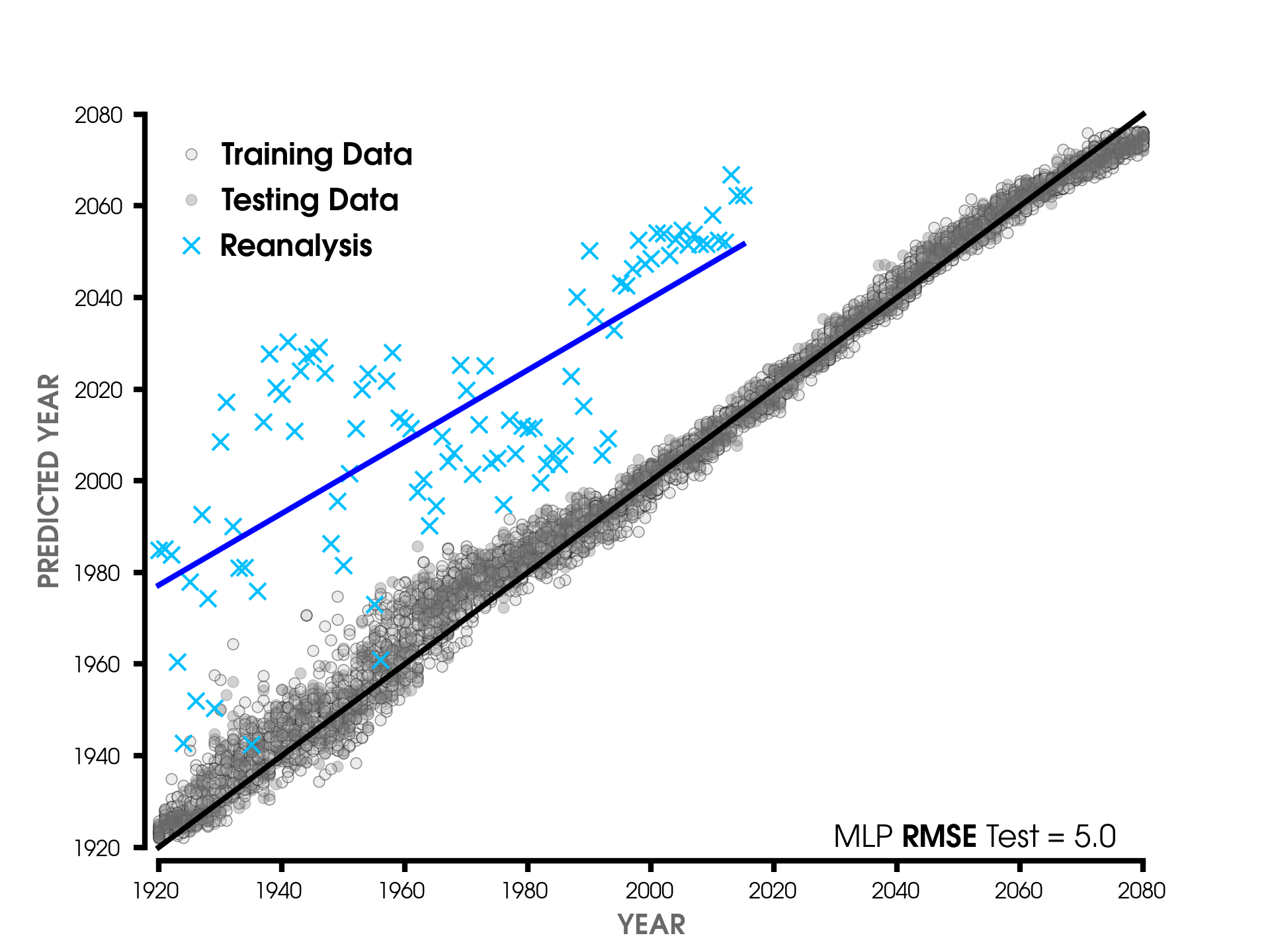
(a)

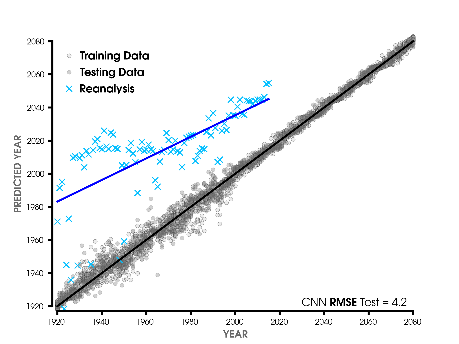
(b)

Figure 9: Network performance based on the RMSE of the predicted years to the true years of both a) MLP and b) CNN (compare to Figure 3c in Labe and Barnes (2021)). The red dots correspond to the agreement of the predictions based on the training and validation data to the actual years and the grey dots show agreement between the predictions on the test set and the actual years, with the black line showing the linear regression across the full model data (training, validation and test data). In blue we also included the predictions on the reanalysis data with the linear regression line in dark blue.

Similar to Labe and Barnes (2021) we show in Figure 9 the regression curves for the model data (grey) and reanalysis data (blue) of A) the MLP and B) CNN. We train both networks such that there are no significant performance differences with test accuracy of $\text{Acc}_{\text{MLP}}=65\pm 4\%$ for the MLP and $\text{Acc}_{\text{CNN}}=70\pm 2\%$ for the CNN (estimated across $50$ trained networks). Additionally, we consider the RMSE of the predicted years and see comparable RSME for the Test Data with $R_{\text{MLP}}=5.0$ and $R_{\text{CNN}}=4.2$.
As we can see in Figure 9, the number of correct predictions changes for different years. Thus, we apply all explanation methods to the full model data $\Omega$, to ensure access to correct samples across all years.

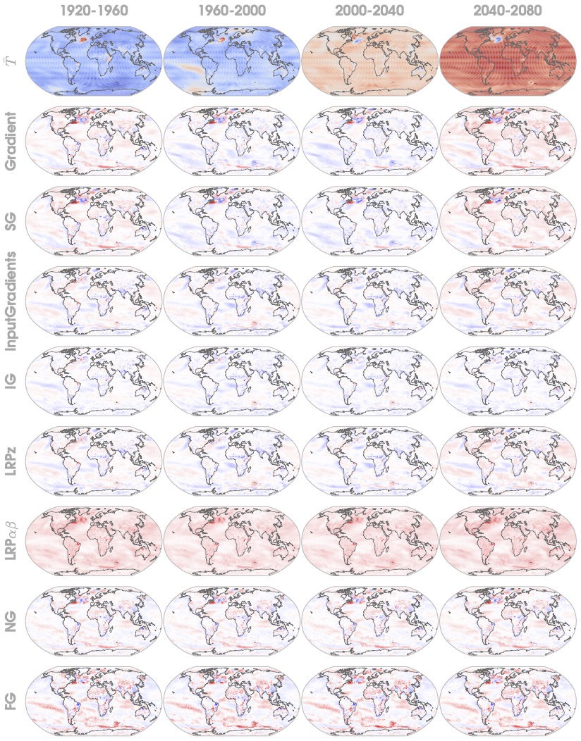
Figure 10: MLP explanation map average over $1920-1960$,$1960-2000$, $2000-2040$ and $2040-2080$ for all XAI methods. The first row shows the average input temperature map $\bar{T}$ with the color bar ranging from maximum (red) to minimum(blue) temperature anomaly. All consecutive lines show the explanation maps of the different XAI methods with color bar ranging from $1$ (red) to $-1$ (blue).

We show examples of for MLP and CNN across all explanation methods in figure 10 and 11. Following Labe and Barnes (2021), we adopt a criterion requiring a correct year regression within an error of $\pm 2$ years, to identify a correct prediction. We average correct predictions across ensemble members and display time periods of $40$ years based on the temporal average of explanations (see Figure 6 in Labe and Barnes (2021)).
In comparison, both figures highlight the difference in spatial learning patterns, with the CNN relevance focusing on pixel groups whereas the MLP relevance can change pixel-wise. In table we list the hyperparameters of the explanation methods, compared in our experiments. We use the notation introduced in Appendix A-A.1. We use IntGrad with the baseline $\bar{\mathbf{x}}$ generated per default by iNNestigate.

Table 4: The hyperparameters of the XAI methods. Note that parameters vary across explanation methods. We report only adjusted parameters, for all others we write $-$. We denote maximum and minimum value across all temperature maps $\mathbf{X}$ in the dataset $\Omega$ as $x_{\text{max}}$ and $x_{\text{min}}$ respectively.

	$\alpha$	$\beta$	$N$	$M$	$\sigma_{\text{SG}}$	$\sigma_{\text{NG}}$	$\Phi_{0}(f(\mathbf{x}))$
FusionGrad	$-$	$-$	$20$	$20$	$0.25(x_{\text{max}}-x_{\text{min}})$	$0.125$	Gradient
InputGradients	$-$	$-$	$-$	$-$	$-$	$-$	$-$
Integrated Gradients	$-$	$-$	$-$	$-$	$-$	$-$	$-$
LRPz	$-$	$-$	$-$	$-$	$-$	$-$	$-$
SmoothGrad	$-$	$-$	$150$	$-$	$0.5(x_{\text{max}}-x_{\text{min}})$	$-$	Gradient
LRPab	$1$	$0$	$-$	$-$	$-$	$-$	$-$
NoiseGrad	$-$	$-$	$-$	$20$	$-$	$0.25$	Gradient
Gradient	$-$	$-$	$-$	$-$	$-$	$-$	$-$

B.2 Evaluation metrics

Hyperparmeters

In table 5 we list the hyperparameters of the different metrics. We list only the adapted parameters for all other (see Hedström et al. (2023)) we used the Quantus default values. The normalisation parameter refers to an explanation normalization according to equation 25.
Faithfulness
In table 5 the perturbation function ’Indices’ refers to the baseline replacement by indices of the highest value pixels in the explanation and ’Linear’ refers to noisy linear imputation (see Rong et al. (2022a) for details).
Randomisation
For the MPT score calculations, we perturb the layer weights starting from the output layer to the input layer, which we refer to as ’bottom$\_$up’ in table 5. To ensure comparability we use the Pearson correlation as the similarity function for both metrics. Localisation
For top-$k$ we consider $k=0.1d$, which are the $10\%$ most relevant pixels of all pixels $d$ in the temperature map.

Table 5: We show the hyperparameters of the XAI evaluation metrics based on the QUANTUS package calculations (Hedström et al., 2023). Note that parameters vary across metrics and we report settings only for metrics with according parameters (for all other we write $-$).

	Robustness		Faithfulness		Randomisation		Complexity		Localisation
Hyperparameters	AS	LLE	FC	ROAD	MPT	RL	Comp.	Spars.	TopK	RRA
Normalization	True	True	True	True	True	True	True	True	True	True
Perturbation function	$\mathcal{N}(0,0.1)$	$\mathcal{N}(0,0.1)$	Indices	Linear	$-$	$-$	$-$	$-$	$-$	$-$
Similarity function	Difference	Lipschitz Constant	Pearson Corr.	$-$	Pearson Corr.	Pearson Corr.	$-$	$-$	$-$	$-$
Num. of samples/runs	$10$	$10$	$50$	$-$	$-$	$-$	$-$	$-$	$-$	$-$
Norm nominator	Frobenius	Euclidean	$-$	$-$	$-$	$-$	$-$	$-$	$-$	$-$
Norm denominator	Frobenius	Euclidean	$-$	$-$	$-$	$-$	$-$	$-$	$-$
Subset size	$-$	$-$	$40$	$-$	$-$	$-$	$-$	$-$	$-$	$-$
Percentage range	$-$	$-$	$-$	$1-50\%$	$-$	$-$	$-$	$-$	$-$
$k$	$-$	$-$	$-$	$-$	$-$	$-$	$-$	$-$	$0.1d$	$-$
Perturbation baseline	$-$	$-$	$U(0,1)$	$U(0,1)$	$-$	$-$	$-$	$-$	$-$	$-$
Number of Classes	$-$	$-$	$-$	$-$	$-$	$20$	$-$	$-$	$-$	$-$
Layer Order	$-$	$-$	$-$	$-$	bottom$\_$up	$-$	$-$	$-$	$-$	$-$

References

- Abadi et al. [2016] M. Abadi, P. Barham, J. Chen, Z. Chen, A. Davis, J. Dean, M. Devin, S. Ghemawat, G. Irving, M. Isard, et al. Tensorflow: a system for large-scale machine learning. In Osdi, volume 16, pages 265–283. Savannah, GA, USA, 2016.
- Adebayo et al. [2018] J. Adebayo, J. Gilmer, M. Muelly, I. Goodfellow, M. Hardt, and B. Kim. Sanity checks for saliency maps. In S. Bengio, H. Wallach, H. Larochelle, K. Grauman, N. Cesa-Bianchi, and R. Garnett, editors, Advances in Neural Information Processing Systems, volume 31. Curran Associates, Inc., 2018. URL https://proceedings.neurips.cc/paper/2018/file/294a8ed24b1ad22ec2e7efea049b8737-Paper.pdf.
- Alber et al. [2019] M. Alber, S. Lapuschkin, P. Seegerer, M. Hägele, K. T. Schütt, G. Montavon, W. Samek, K.-R. Müller, S. Dähne, and P.-J. Kindermans. innvestigate neural networks! Journal of Machine Learning Research, 20(93):1–8, 2019. URL http://jmlr.org/papers/v20/18-540.html.
- Alvarez-Melis and Jaakkola [2018] D. Alvarez-Melis and T. S. Jaakkola. On the robustness of interpretability methods. arXiv preprint arXiv:1806.08049, 2018.
- Anantrasirichai et al. [2019] N. Anantrasirichai, J. Biggs, F. Albino, and D. Bull. A deep learning approach to detecting volcano deformation from satellite imagery using synthetic datasets. Remote Sensing of Environment, 230:111179, sep 2019. doi: 10.1016/j.rse.2019.04.032.
- Arias-Duart et al. [2022] A. Arias-Duart, F. Parés, D. Garcia-Gasulla, and V. Giménez-Ábalos. Focus! rating xai methods and finding biases. In 2022 IEEE International Conference on Fuzzy Systems (FUZZ-IEEE), pages 1–8, 2022. doi: 10.1109/FUZZ-IEEE55066.2022.9882821.
- Arras et al. [2022] L. Arras, A. Osman, and W. Samek. Clevr-xai: A benchmark dataset for the ground truth evaluation of neural network explanations. Information Fusion, 81:14–40, 2022. ISSN 1566-2535. doi: https://doi.org/10.1016/j.inffus.2021.11.008. URL https://www.sciencedirect.com/science/article/pii/S1566253521002335.
- Arrieta et al. [2020] A. B. Arrieta, N. Díaz-Rodríguez, J. D. Ser, A. Bennetot, S. Tabik, A. Barbado, S. Garcia, S. Gil-Lopez, D. Molina, R. Benjamins, R. Chatila, and F. Herrera. Explainable artificial intelligence (XAI): Concepts, taxonomies, opportunities and challenges toward responsible AI. Information Fusion, 58:82–115, jun 2020. doi: 10.1016/j.inffus.2019.12.012.
- Bach et al. [2015] S. Bach, A. Binder, G. Montavon, F. Klauschen, K.-R. Müller, and W. Samek. On pixel-wise explanations for non-linear classifier decisions by layer-wise relevance propagation. PLOS ONE, 10(7):e0130140, jul 2015. doi: 10.1371/journal.pone.0130140.
- Baehrens et al. [2010] D. Baehrens, T. Schroeter, S. Harmeling, M. Kawanabe, K. Hansen, and K.-R. Müller. How to explain individual classification decisions. J. Mach. Learn. Res., 11:1803–1831, aug 2010. ISSN 1532-4435.
- Bhatt et al. [2020] U. Bhatt, A. Weller, and J. M. Moura. Evaluating and aggregating feature-based model explanations. arXiv preprint arXiv:2005.00631, 2020.
- Brocki and Chung [2022] L. Brocki and N. C. Chung. Evaluation of interpretability methods and perturbation artifacts in deep neural networks. CoRR, abs/2203.02928, 2022. doi: 10.48550/arXiv.2203.02928.
- Bromberg et al. [2019] C. L. Bromberg, C. Gazen, J. J. Hickey, J. Burge, L. Barrington, and S. Agrawal. Machine learning for precipitation nowcasting from radar images. ArXiv, abs/1912.12132:4, 2019.
- Bykov et al. [2021] K. Bykov, M. M. C. Höhne, A. Creosteanu, K.-R. Müller, F. Klauschen, S. Nakajima, and M. Kloft. Explaining bayesian neural networks. arXiv preprint arXiv:2108.10346, Aug. 2021.
- Bykov et al. [2022] K. Bykov, A. Hedström, S. Nakajima, and M. M.-C. Höhne. Noisegrad—enhancing explanations by introducing stochasticity to model weights. In Proceedings of the AAAI Conference on Artificial Intelligence, volume 36, pages 6132–6140, 2022.
- Camps-Valls et al. [2020] G. Camps-Valls, M. Reichstein, X. Zhu, and D. Tuia. Advancing Deep Learning for Earth Sciences From Hybrid Modeling To Interpretability. In IEEE International Geoscience and Remote Sensing Symposium, IGARSS 2020, Waikoloa, HI, USA, September 26 - October 2, 2020, pages 3979–3982. IEEE, 2020. doi: 10.1109/IGARSS39084.2020.9323558.
- Caswell et al. [2020] T. A. Caswell, M. Droettboom, A. Lee, J. Hunter, E. Firing, D. Stansby, J. Klymak, T. Hoffmann, E. S. D. Andrade, N. Varoquaux, J. H. Nielsen, B. Root, P. Elson, R. May, D. Dale, Jae-Joon Lee, J. K. Seppänen, D. McDougall, A. Straw, P. Hobson, C. Gohlke, T. S. Yu, E. Ma, A. F. Vincent, S. Silvester, C. Moad, N. Kniazev, P. Ivanov, E. Ernest, and J. Katins. matplotlib/matplotlib: Rel: v3.2.1, 2020.
- Chalasani et al. [2020] P. Chalasani, J. Chen, A. R. Chowdhury, S. Jha, and X. Wu. Concise explanations of neural networks using adversarial training. In Proceedings of the 37th International Conference on Machine Learning, ICML’20. JMLR.org, 2020.
- Chen et al. [2019] C. Chen, O. Li, D. Tao, A. Barnett, C. Rudin, and J. K. Su. This looks like that: Deep learning for interpretable image recognition. In H. Wallach, H. Larochelle, A. Beygelzimer, F. d'Alché-Buc, E. Fox, and R. Garnett, editors, Advances in Neural Information Processing Systems, volume 32. Curran Associates, Inc., 2019. URL https://proceedings.neurips.cc/paper/2019/file/adf7ee2dcf142b0e11888e72b43fcb75-Paper.pdf.
- Chen et al. [2020] K. Chen, P. Wang, X. Yang, N. Zhang, and D. Wang. A model output deep learning method for grid temperature forecasts in tianjin area. Applied Sciences, 10(17):5808, aug 2020. doi: 10.3390/app10175808.
- Clare et al. [2022] M. C. Clare, M. Sonnewald, R. Lguensat, J. Deshayes, and V. Balaji. Explainable artificial intelligence for bayesian neural networks: toward trustworthy predictions of ocean dynamics. Journal of Advances in Modeling Earth Systems, 14(11):e2022MS003162, 2022. doi: 10.1002/essoar.10511239.1.
- Commission et al. [2019] E. Commission, C. Directorate-General for Communications Networks, and Technology. Ethics guidelines for trustworthy AI. Publications Office, 2019. doi: doi/10.2759/346720.
- Dikshit and Pradhan [2021] A. Dikshit and B. Pradhan. Interpretable and explainable AI (XAI) model for spatial drought prediction. Science of The Total Environment, 801:149797, dec 2021. doi: 10.1016/j.scitotenv.2021.149797.
- Ebert-Uphoff and Hilburn [2020] I. Ebert-Uphoff and K. Hilburn. Evaluation, tuning, and interpretation of neural networks for working with images in meteorological applications. Bulletin of the American Meteorological Society, 101(12):E2149 – E2170, 2020. doi: 10.1175/BAMS-D-20-0097.1. URL https://journals.ametsoc.org/view/journals/bams/101/12/BAMS-D-20-0097.1.xml.
- Gautam et al. [2022] S. Gautam, A. Boubekki, S. Hansen, S. A. Salahuddin, R. Jenssen, M. M.-C. Höhne, and M. Kampffmeyer. Protovae: A trustworthy self-explainable prototypical variational model. In Advances in Neural Information Processing Systems, 2022.
- Gautam et al. [2023] S. Gautam, M. M.-C. Höhne, S. Hansen, R. Jenssen, and M. Kampffmeyer. This looks more like that: Enhancing self-explaining models by prototypical relevance propagation. Pattern Recognition, 136:109172, 2023.
- Gevaert et al. [2022] A. Gevaert, A. Rousseau, T. Becker, D. Valkenborg, T. D. Bie, and Y. Saeys. Evaluating feature attribution methods in the image domain. CoRR, abs/2202.12270, 2022. URL https://arxiv.org/abs/2202.12270.
- Gibson et al. [2021] P. B. Gibson, W. E. Chapman, A. Altinok, L. D. Monache, M. J. DeFlorio, and D. E. Waliser. Training machine learning models on climate model output yields skillful interpretable seasonal precipitation forecasts. Communications Earth & amp Environment, 2(1), aug 2021. doi: 10.1038/s43247-021-00225-4.
- Grinwald et al. [2022] D. Grinwald, K. Bykov, S. Nakajima, and M. M.-C. Höhne. Visualizing the diversity of representations learned by bayesian neural networks. arXiv preprint arXiv:2201.10859, 2022.
- Ham et al. [2019] Y.-G. Ham, J.-H. Kim, and J.-J. Luo. Deep learning for multi-year ENSO forecasts. Nature, 573(7775):568–572, sep 2019. doi: 10.1038/s41586-019-1559-7.
- Han et al. [2017] L. Han, J. Sun, W. Zhang, Y. Xiu, H. Feng, and Y. Lin. A machine learning nowcasting method based on real-time reanalysis data. Journal of Geophysical Research: Atmospheres, 122(7):4038–4051, apr 2017. doi: 10.1002/2016jd025783.
- Harder et al. [2021] P. Harder, D. Watson-Parris, D. Strassel, N. Gauger, P. Stier, and J. Keuper. Emulating aerosol microphysics with a machine learning. In ICML 2021 Workshop on Tackling Climate Change with Machine Learning, 2021. URL https://www.climatechange.ai/papers/icml2021/24.
- Harris et al. [2020] C. Harris, K. Millman, S. Walt, R. Gommers, P. Virtanen, D. Cournapeau, E. Wieser, J. Taylor, S. Berg, N. Smith, R. Kern, M. Picus, S. Hoyer, M. Kerkwijk, M. Brett, A. Haldane, J. Río, M. Wiebe, P. Peterson, and T. Oliphant. Array programming with numpy. Nature, 585:357–362, 09 2020. doi: 10.1038/s41586-020-2649-2.
- Hedström et al. [2023] A. Hedström, L. Weber, F. Motzkus, W. Samek, S. Lapuschkin, and M. M.-C. Höhne. Quantus: An explainable ai toolkit for responsible evaluation of neural network explanations and beyond. Journal of Machine Learning Research, 24(34):1–11, 2023.
- Hengl et al. [2017] T. Hengl, J. M. de Jesus, G. B. M. Heuvelink, M. R. Gonzalez, M. Kilibarda, A. Blagotić, W. Shangguan, M. N. Wright, X. Geng, B. Bauer-Marschallinger, M. A. Guevara, R. Vargas, R. A. MacMillan, N. H. Batjes, J. G. B. Leenaars, E. Ribeiro, I. Wheeler, S. Mantel, and B. Kempen. SoilGrids250m: Global gridded soil information based on machine learning. PLOS ONE, 12(2):e0169748, feb 2017. doi: 10.1371/journal.pone.0169748.
- Hilburn et al. [2021] K. A. Hilburn, I. Ebert-Uphoff, and S. D. Miller. Development and interpretation of a neural-network-based synthetic radar reflectivity estimator using goes-r satellite observations. Journal of Applied Meteorology and Climatology, 60(1):3 – 21, 2021. doi: 10.1175/JAMC-D-20-0084.1. URL https://journals.ametsoc.org/view/journals/apme/60/1/jamc-d-20-0084.1.xml.
- Hoffman et al. [2018] R. R. Hoffman, S. T. Mueller, G. Klein, and J. Litman. Metrics for explainable ai: Challenges and prospects. ArXiv, abs/1812.04608, Dec. 2018.
- Hurley and Rickard [2009] N. Hurley and S. Rickard. Comparing measures of sparsity. Information Theory, IEEE Transactions on, 55:4723 – 4741, 11 2009. doi: 10.1109/TIT.2009.2027527.
- Hurrell et al. [2013] J. W. Hurrell, M. M. Holland, P. R. Gent, S. Ghan, J. E. Kay, P. J. Kushner, J.-F. Lamarque, W. G. Large, D. Lawrence, K. Lindsay, W. H. Lipscomb, M. C. Long, N. Mahowald, D. R. Marsh, R. B. Neale, P. Rasch, S. Vavrus, M. Vertenstein, D. Bader, W. D. Collins, J. J. Hack, J. Kiehl, and S. Marshall. The community earth system model: A framework for collaborative research. Bulletin of the American Meteorological Society, 94(9):1339–1360, sep 2013. doi: 10.1175/bams-d-12-00121.1.
- Kay et al. [2015] J. E. Kay, C. Deser, A. Phillips, A. Mai, C. Hannay, G. Strand, J. M. Arblaster, S. C. Bates, G. Danabasoglu, J. Edwards, M. Holland, P. Kushner, J.-F. Lamarque, D. Lawrence, K. Lindsay, A. Middleton, E. Munoz, R. Neale, K. Oleson, L. Polvani, and M. Vertenstein. The community earth system model (CESM) large ensemble project: A community resource for studying climate change in the presence of internal climate variability. Bulletin of the American Meteorological Society, 96(8):1333–1349, aug 2015. doi: 10.1175/bams-d-13-00255.1.
- Krishna et al. [2022] S. Krishna, T. Han, A. Gu, J. Pombra, S. Jabbari, S. Wu, and H. Lakkaraju. The disagreement problem in explainable machine learning: A practitioner’s perspective. CoRR, abs/2202.01602, 2022. URL https://arxiv.org/abs/2202.01602.
- Labe and Barnes [2021] Z. M. Labe and E. A. Barnes. Detecting climate signals using explainable AI with single-forcing large ensembles. Journal of Advances in Modeling Earth Systems, 13(6), jun 2021. doi: 10.1029/2021ms002464.
- Labe and Barnes [2022] Z. M. Labe and E. A. Barnes. Comparison of Climate Model Large Ensembles With Observations in the Arctic Using Simple Neural Networks. Earth and Space Science, 9(7):e02348, July 2022. doi: 10.1002/essoar.10510977.1.
- Lapuschkin et al. [2019] S. Lapuschkin, S. Wäldchen, A. Binder, G. Montavon, W. Samek, and K.-R. Müller. Unmasking clever hans predictors and assessing what machines really learn. Nature communications, 10(1):1096, 2019.
- Leavitt and Morcos [2020] M. L. Leavitt and A. S. Morcos. Towards falsifiable interpretability research. CoRR, abs/2010.12016, 2020. URL https://arxiv.org/abs/2010.12016.
- Leinonen et al. [2021] J. Leinonen, D. Nerini, and A. Berne. Stochastic super-resolution for downscaling time-evolving atmospheric fields with a generative adversarial network. IEEE Transactions on Geoscience and Remote Sensing, 59(9):7211–7223, sep 2021. doi: 10.1109/tgrs.2020.3032790.
- Letzgus et al. [2022] S. Letzgus, P. Wagner, J. Lederer, W. Samek, K.-R. Muller, and G. Montavon. Toward Explainable Artificial Intelligence for Regression Models: A methodological perspective. IEEE Signal Processing Magazine, 39(4):40–58, July 2022. doi: 10.1109/MSP.2022.3153277.
- Mamalakis et al. [2021] A. Mamalakis, I. Ebert-Uphoff, and E. A. Barnes. Neural network attribution methods for problems in geoscience: A novel synthetic benchmark dataset. Environmental Data Science, Mar. 2021.
- Mamalakis et al. [2022] A. Mamalakis, E. A. Barnes, and I. Ebert-Uphoff. Investigating the fidelity of explainable artificial intelligence methods for applications of convolutional neural networks in geoscience. Artificial Intelligence for the Earth Systems, pages 1–42, aug 2022. doi: 10.1175/aies-d-22-0012.1.
- Mayer and Barnes [2021] K. J. Mayer and E. A. Barnes. Subseasonal forecasts of opportunity identified by an explainable neural network. Geophysical Research Letters, 48(10), may 2021. doi: 10.1029/2020gl092092.
- McGovern et al. [2019] A. McGovern, R. Lagerquist, D. J. Gagne, G. E. Jergensen, K. L. Elmore, C. R. Homeyer, and T. Smith. Making the black box more transparent: Understanding the physical implications of machine learning. Bulletin of the American Meteorological Society, 100(11):2175–2199, nov 2019. doi: 10.1175/bams-d-18-0195.1.
- Mohseni et al. [2021] S. Mohseni, N. Zarei, and E. D. Ragan. A multidisciplinary survey and framework for design and evaluation of explainable AI systems. ACM Transactions on Interactive Intelligent Systems, 11(3-4):1–45, dec 2021. doi: 10.1145/3387166.
- Montavon et al. [2017] G. Montavon, S. Lapuschkin, A. Binder, W. Samek, and K.-R. Müller. Explaining nonlinear classification decisions with deep taylor decomposition. Pattern Recognition, 65:211–222, may 2017. doi: 10.1016/j.patcog.2016.11.008.
- Montavon et al. [2018] G. Montavon, W. Samek, and K.-R. Müller. Methods for interpreting and understanding deep neural networks. Digital Signal Processing, 73:1–15, feb 2018. doi: 10.1016/j.dsp.2017.10.011.
- Montavon et al. [2019] G. Montavon, A. Binder, S. Lapuschkin, W. Samek, and K.-R. Müller. Layer-Wise Relevance Propagation: An Overview, pages 193–209. Lecture Notes in Computer Science (including subseries Lecture Notes in Artificial Intelligence and Lecture Notes in Bioinformatics). Springer Verlag, 2019. doi: 10.1007/978-3-030-28954-6˙10.
- Nguyen et al. [2016] A. M. Nguyen, A. Dosovitskiy, J. Yosinski, T. Brox, and J. Clune. Synthesizing the preferred inputs for neurons in neural networks via deep generator networks. In D. D. Lee, M. Sugiyama, U. von Luxburg, I. Guyon, and R. Garnett, editors, Advances in Neural Information Processing Systems 29: Annual Conference on Neural Information Processing Systems 2016, December 5-10, 2016, Barcelona, Spain, pages 3387–3395, 2016. URL https://proceedings.neurips.cc/paper/2016/hash/5d79099fcdf499f12b79770834c0164a-Abstract.html.
- Pegion et al. [2022] K. Pegion, E. J. Becker, and B. P. Kirtman. Understanding predictability of daily southeast u.s. precipitation using explainable machine learning. Artificial Intelligence for the Earth Systems, 1(4), oct 2022. doi: 10.1175/aies-d-22-0011.1.
- phi Nguyen and Martinez [2020] A. phi Nguyen and M. R. Martinez. On quantitative aspects of model interpretability. ArXiv, abs/2007.07584, 2020.
- Ribeiro et al. [2016] M. T. Ribeiro, S. Singh, and C. Guestrin. ” why should i trust you?” explaining the predictions of any classifier. In Proceedings of the 22nd ACM SIGKDD international conference on knowledge discovery and data mining, pages 1135–1144, 2016.
- Rieger and Hansen [2020] L. Rieger and L. K. Hansen. IROF: a low resource evaluation metric for explanation methods. CoRR, abs/2003.08747, 2020. URL https://arxiv.org/abs/2003.08747.
- Rong et al. [2022a] Y. Rong, T. Leemann, V. Borisov, G. Kasneci, and E. Kasneci. A consistent and efficient evaluation strategy for attribution methods. In K. Chaudhuri, S. Jegelka, L. Song, C. Szepesvari, G. Niu, and S. Sabato, editors, Proceedings of the 39th International Conference on Machine Learning, volume 162 of Proceedings of Machine Learning Research, pages 18770–18795. PMLR, 17–23 Jul 2022a. URL https://proceedings.mlr.press/v162/rong22a.html.
- Rong et al. [2022b] Y. Rong, T. Leemann, V. Borisov, G. Kasneci, and E. Kasneci. Evaluating feature attribution: An information-theoretic perspective. CoRR, abs/2202.00449, 2022b. URL https://arxiv.org/abs/2202.00449.
- Samek et al. [2017] W. Samek, A. Binder, G. Montavon, S. Lapuschkin, and K.-R. Muller. Evaluating the visualization of what a deep neural network has learned. IEEE transactions on neural networks and learning systems, 28:2660–2673, Nov. 2017. ISSN 2162-2388. doi: 10.1109/TNNLS.2016.2599820.
- Scher and Messori [2021] S. Scher and G. Messori. Ensemble methods for neural network-based weather forecasts. Journal of Advances in Modeling Earth Systems, 13(2), feb 2021. doi: 10.1029/2020ms002331.
- Shi et al. [2015] X. Shi, Z. Chen, H. Wang, D.-Y. Yeung, W.-K. Wong, and W.-c. Woo. Convolutional lstm network: A machine learning approach for precipitation nowcasting. Advances in neural information processing systems, 28, 2015.
- Simonyan et al. [2014] K. Simonyan, A. Vedaldi, and A. Zisserman. Deep inside convolutional networks: Visualising image classification models and saliency maps. In Y. Bengio and Y. LeCun, editors, 2nd International Conference on Learning Representations, ICLR 2014, Banff, AB, Canada, April 14-16, 2014, Workshop Track Proceedings, 2014. URL http://arxiv.org/abs/1312.6034.
- Sixt et al. [2020] L. Sixt, M. Granz, and T. Landgraf. When explanations lie: Why many modified BP attributions fail. In H. D. III and A. Singh, editors, Proceedings of the 37th International Conference on Machine Learning, volume 119 of Proceedings of Machine Learning Research, pages 9046–9057. PMLR, 13–18 Jul 2020. URL https://proceedings.mlr.press/v119/sixt20a.html.
- Slivinski et al. [2019] L. C. Slivinski, G. P. Compo, J. S. Whitaker, P. D. Sardeshmukh, B. S. Giese, C. McColl, R. Allan, X. Yin, R. Vose, H. Titchner, J. Kennedy, L. J. Spencer, L. Ashcroft, S. Brönnimann, M. Brunet, D. Camuffo, R. Cornes, T. A. Cram, R. Crouthamel, F. Domínguez-Castro, J. E. Freeman, J. Gergis, E. Hawkins, P. D. Jones, S. Jourdain, A. Kaplan, H. Kubota, F. L. Blancq, T.-C. Lee, A. Lorrey, J. Luterbacher, M. Maugeri, C. J. Mock, G. K. Moore, R. Przybylak, C. Pudmenzky, C. Reason, V. C. Slonosky, C. A. Smith, B. Tinz, B. Trewin, M. A. Valente, X. L. Wang, C. Wilkinson, K. Wood, and P. Wyszyński. Towards a more reliable historical reanalysis: Improvements for version 3 of the twentieth century reanalysis system. Quarterly Journal of the Royal Meteorological Society, 145(724):2876–2908, aug 2019. doi: 10.1002/qj.3598.
- Smilkov et al. [2017] D. Smilkov, N. Thorat, B. Kim, F. B. Viégas, and M. Wattenberg. Smoothgrad: removing noise by adding noise. CoRR, abs/1706.03825, 2017. URL http://arxiv.org/abs/1706.03825.
- Sonnewald and Lguensat [2021] M. Sonnewald and R. Lguensat. Revealing the impact of global heating on north atlantic circulation using transparent machine learning. Journal of Advances in Modeling Earth Systems, 13(8), aug 2021. doi: 10.1029/2021ms002496.
- Strumbelj and Kononenko [2010] E. Strumbelj and I. Kononenko. An efficient explanation of individual classifications using game theory. The Journal of Machine Learning Research, 11:1–18, 2010.
- Sundararajan et al. [2017] M. Sundararajan, A. Taly, and Q. Yan. Axiomatic attribution for deep networks. In International conference on machine learning, pages 3319–3328. PMLR, 2017.
- Theiner et al. [2022] J. Theiner, E. Müller-Budack, and R. Ewerth. Interpretable semantic photo geolocation. In Proceedings of the IEEE/CVF Winter Conference on Applications of Computer Vision (WACV), pages 750–760, January 2022.
- Thiebes et al. [2020] S. Thiebes, S. Lins, and A. Sunyaev. Trustworthy artificial intelligence. Electronic Markets, 31(2):447–464, oct 2020. doi: 10.1007/s12525-020-00441-4.
- Tomsett et al. [2022] R. Tomsett, D. Harborne, S. Chakraborty, P. Gurram, and A. Preece. Sanity checks for saliency metrics. Proceedings of the AAAI Conference on Artificial Intelligence, 34:6021–6029, 2022. ISSN 2374-3468. doi: 10.1609/aaai.v34i04.6064.
- van Straaten et al. [2022] C. van Straaten, K. Whan, D. Coumou, B. van den Hurk, and M. Schmeits. Using explainable machine learning forecasts to discover subseasonal drivers of high summer temperatures in western and central europe. Monthly Weather Review, 150(5):1115–1134, may 2022. doi: 10.1175/mwr-d-21-0201.1.
- Vidovic et al. [2015] M. M.-C. Vidovic, N. Görnitz, K.-R. Müller, G. Rätsch, and M. Kloft. Opening the black box: Revealing interpretable sequence motifs in kernel-based learning algorithms. In Machine Learning and Knowledge Discovery in Databases: European Conference, ECML PKDD 2015, Porto, Portugal, September 7-11, 2015, Proceedings, Part II 15, pages 137–153. Springer, 2015.
- Vidovic et al. [2016] M. M.-C. Vidovic, N. Görnitz, K.-R. Müller, and M. Kloft. Feature importance measure for non-linear learning algorithms. arXiv preprint arXiv:1611.07567, 2016.
- Virtanen et al. [2020] P. Virtanen, R. Gommers, T. E. Oliphant, M. Haberland, T. Reddy, D. Cournapeau, E. Burovski, P. Peterson, W. Weckesser, J. Bright, et al. Scipy 1.0: fundamental algorithms for scientific computing in python. Nature methods, 17:261–272, 2020.
- Wang et al. [2021] J. Wang, K. Gao, Z. Zhang, C. Ni, Z. Hu, D. Chen, and Q. Wu. Multisensor remote sensing imagery super-resolution with conditional GAN. Journal of Remote Sensing, 2021:1–11, sep 2021. doi: 10.34133/2021/9829706.
- Yeh et al. [2019] C.-K. Yeh, C.-Y. Hsieh, A. Suggala, D. I. Inouye, and P. K. Ravikumar. On the (in)fidelity and sensitivity of explanations. In Advances in Neural Information Processing Systems, volume 32. Curran Associates, Inc., 2019. URL https://proceedings.neurips.cc/paper/2019/file/a7471fdc77b3435276507cc8f2dc2569-Paper.pdf.
- Yuval and O’Gorman [2020] J. Yuval and P. A. O’Gorman. Stable machine-learning parameterization of subgrid processes for climate modeling at a range of resolutions. Nature Communications, 11(1), jul 2020. doi: 10.1038/s41467-020-17142-3.
- Zhang et al. [2018] J. Zhang, S. A. Bargal, Z. Lin, J. Brandt, X. Shen, and S. Sclaroff. Top-down neural attention by excitation backprop. International Journal of Computer Vision, 126(10):1084–1102, 2018.