CausIL: Causal Graph for Instance Level Microservice Data

Abstract.

AI-based monitoring has become crucial for cloud-based services due to its scale. A common approach to AI-based monitoring is to detect causal relationships among service components and build a causal graph. Availability of domain information makes cloud systems even better suited for such causal detection approaches. In modern cloud systems, however, auto-scalers dynamically change the number of microservice instances, and a load-balancer manages the load on each instance. This poses a challenge for off-the-shelf causal structure detection techniques as they neither incorporate the system architectural domain information nor provide a way to model distributed compute across varying numbers of service instances. To address this, we develop CausIL, which detects a causal structure among service metrics by considering compute distributed across dynamic instances and incorporating domain knowledge derived from system architecture. Towards the application in cloud systems, CausIL estimates a causal graph using instance-specific variations in performance metrics, modeling multiple instances of a service as independent, conditional on system assumptions. Simulation study shows the efficacy of CausIL over baselines by improving graph estimation accuracy by $\sim$25% as measured by Structural Hamming Distance whereas the real-world dataset demonstrates CausIL’s applicability in deployment settings.

1. Introduction

Modern cloud-based applications follow a microservice architecture (Balalaie et al., 2016), consisting of a large number of components connected through complex dependencies (net, 2015; ube, 2021) that run in a distributed environment. These applications have a simple development process and flexible deployment in general (Newman, 2021). A modern microservice ecosystem (Nadareishvili et al., 2016) deploys multiple instances of the same service (which are sometimes referred to as pods (pod, 2022), though similar in meaning) and often increases and decreases their number in response to the change in the load and utilization. The number of unique instances is numerous, short-lived and varying over time. As an illustrative example, in a small microservice at Adobe, 1117 unique instances were spawned within 3 months, with an average of 8 instances active at any time instant. The median life of the instances was only 350 mins. Auto-scalers are configured to automatically scale the number of instances up or down depending on the load and utilization, and a load balancer manages and distributes the load to each of these instances. Due to their large scale and complexity, such architectures are vulnerable to failures. Hence, to maintain the availability and reliability of the system, an accurate structural understanding of the system is required to perform multiple performance diagnosis tasks (Chen et al., 2014; Meng et al., 2020; Liu et al., 2021; Laguna et al., 2013; Nguyen et al., 2011, 2013; Chen et al., 2019).

Building a causal dependency graph to represent system architecture is an approach being used extensively (Chen et al., 2014, 2019; Liu et al., 2021; Wu et al., 2021; Ikram et al., 2022) in the domain of performance diagnosis. Each deployed instance of a microservice is monitored by numerous system indicator metrics (Coburn Watson and Gregg, 2022) like load request, resource utilization, HTTP errors, etc., thus resulting in thousands of such metrics for an entire system. The objective is to learn a graph with causal dependencies among all these metrics using causal structure estimation approaches, such that metrics form the nodes and edge $(a,b)$ denotes that metric $a$ causally affects metric $b$. A failure in one metric can be traced back to the subsequent anomalies in other metrics across multiple microservices using the discovered causal graph.

With multiple instances getting deployed and remaining active for a microservice, it is natural to use metrics from each of the instances in the causal structure estimation. Aggregating metric values over all instances reduce the instance-specific variations of metrics, hence losing a significant amount of information (Moghimi and Corley, 2020), which even we show in §4.2.2 and §6. However, none of the off-the-shelf causal discovery algorithms (Spirtes et al., 2000; Ramsey et al., 2017; Liu et al., 2021) can handle the task of instance-level causal structure learning. Past works (Chen et al., 2014; Gan et al., 2021; Li et al., 2022; Meng et al., 2020) build a causal graph only at an aggregate level and overlook the deployment strategy of microservices over multiple instances. However, even a few instances failing can degrade the quality of service, which might not be captured in an aggregate statistics. Hence, one must perform a diagnosis at the instance level, which can only be possible by capturing instance-specific variations in a causal graph. However, with each instance being short-lived and the total number of instances varying over time, modeling at instance-level is a challenging task, which we aim to solve.

In this work, we propose a novel instance-specific causal structure estimation algorithm, which to the best of our knowledge is the first-of-its-kind, that considers metric variations for each instance deployed per service while building the causal structure, implicitly modeling the decisions of auto-scalers and load balancers. It further incorporates domain knowledge backed by system-based metric semantics combined with intuitive assumptions in a scalable way to improve the accuracy of the structure detection algorithm. We call our approach Causal Structure Detection using Instance Level Simulation CausIL. We have made our code publicly available. We validate our approach on synthetic and semi-synthetic datasets, on which it outperforms the baselines by $\sim 25\%$. We also observe that a large impact is seen by incorporating domain knowledge where accuracy improves by $3.5\times$, as measured by Structural Hamming Distance. We further validate CausIL on a real-world dataset and show performance gain against baselines. The contributions of our work can be summarized as:

1. We study multiple ways of incorporating instance-specific variations in metrics including aggregation strategies and discuss their shortcomings empirically

2. We propose a novel causal structural detection algorithm at the instance level (CausIL) to model instance-level data for microservices. It accounts for multiple data points belonging to multiple instances at each time period due to distributed compute (load-balancer) as well as can model the dynamic number of instances (spawned by an autoscaler), wherein each instance can be short-lived.

3. Domain Knowledge Inclusion: Based on practical assumptions derived from the service dependency graph and metric semantics, we provide a list of general rules in the form of prohibited edges along with ways to incorporate them in CausIL to improve computation time and accuracy.

2. Related Work

With the recent upsurge of work in the field of performance diagnosis of large and complex modern microservice architectures (Chen et al., 2014; Meng et al., 2020; Mondal et al., 2021; Brandón et al., 2020; Ikram et al., 2022), researchers at many cloud-based companies are actively working on alerting and monitoring solutions  (Chen et al., 2019; Wang et al., 2019; Li et al., 2020). Alerting services like Watchdog, New Relic and Splunk diagnose systems by constructing causal graphs between services or using thresholding techniques. These service (new, 2019) monitor performance for each instance by setting alerts for each instance deployed for a microservice. As a result, service reliability tools that use causal dependency graphs should use instance-level data rather than aggregated data for accurate representation. This also allows for the identification and isolation of issues that would otherwise go unnoticed with aggregated data.

Initial works (Nguyen et al., 2013, 2011) have built dependency graphs among services (also called as service call graphs) to diagnose performance during faults, which show control flow from one service to another, which allow analysis of faults at the service level granularity, that is identifying which service is faulty. Service dependency graphs are also used to answer “what-if” based system questions on bandwidth management and application latencies (Tariq et al., 2008, 2013; Jiang et al., 2016; Hu et al., 2018). Grano (Wang et al., 2019) builds a causal dependency graph among physical resources for fault diagnosis. However, performance diagnosis is often demanded at a more granular level.

Multiple works (Chen et al., 2014; Meng et al., 2020; Wu et al., 2021; Wang et al., 2018, 2021) aim to build a causal graph at the performance metric level to diagnose a system in terms of faulty metrics of a service. They utilize the PC algorithm  (Spirtes et al., 2000), a causal structure estimation algorithm, to construct a causal dependency graph at the performance metric level, with each metric representing a node. (Meng et al., 2020) proposed a variation of the PC algorithm to build the causal graph by utilizing the temporal relationships between the metrics of various services. Other nuances in causal graph construction involves using knowledge graph in conjunction with PC algorithm (Qiu et al., 2020), or using alerts which are triggered when a metric crosses a threshold (Chen et al., 2019). However, these approaches are agnostic to the deployment strategy of a microservice which involves multiple instances being spawned and auto-scaled for load-balancing.During a high-load period, aggregating information across all deployed instances to construct the causal graph can result in information loss. (Moghimi and Corley, 2020). Understanding instance-specific metric variations is critical for better capturing system state.

Furthermore, incorporating knowledge of the system architecture can improve the accuracy of the estimated causal graph by removing unnecessary or redundant connections between metrics and enforcing connections that are inherent in microservice systems. Some works (Gan et al., 2021; Li et al., 2022) have developed a causal Bayesian network of the system using system knowledge and causal assumptions. However, to the best of our knowledge, no previous studies have combined instance-level variations in metric data with system knowledge to estimate a causal graph at the performance metric level, which is the main contribution of our research.

3. Problem Formulation

3.1. Preliminaries

A causal structure for a microservice based application (also called dependency graph) is built either with nodes as services or as various performance metrics like latency, load request, utilization etc. The latter approach provides a richer understanding of the entire system and fault localization can be achieved at a more granular level (Chen et al., 2014; Wang et al., 2018; Meng et al., 2020; Ikram et al., 2022) by indicating that a particular metric of a service is faulty. Our solution utilizes the second approach, with a causal graph at the metric level (Fig. 1) where nodes will indicate a set of performance metrics (denoted as parent set for a metric) being responsible for causally influencing an affected metric. Throughout this paper, we have interchangeably used the term service and microservice.

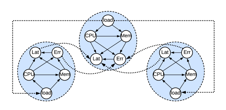
[Causal Dependency Graph among performance metrics]A causal graph between performance metrics of multiple services where workload, error and latency metrics are connected across services.

Figure 1. Causal dependency graph between performance metrics of 3 services. Each service is denoted by a dotted blue circle. Dotted lines indicate dependencies that span across services. The white solid circles are the performance metrics.

3.1.1. Causal Graph Structure

Let $\mathcal{G}(V,E)$ be a causal graph (directed acyclic graph DAG) where the set of nodes $V$ are the metrics observed in the system, and $E$ are the causal edges between those metrics. An edge $v_{i}\rightarrow v_{j}$, where $v_{i},v_{j}\in V$ in $\mathcal{G}$ denote that metric $v_{i}$ is the cause for the metric $v_{j}$ and $v_{j}\mathchoice{\mathrel{\hbox to0.0pt{$\displaystyle\perp$\hss}\mkern 2.0mu{\displaystyle\perp}}}{\mathrel{\hbox to0.0pt{$\textstyle\perp$\hss}\mkern 2.0mu{\textstyle\perp}}}{\mathrel{\hbox to0.0pt{$\scriptstyle\perp$\hss}\mkern 2.0mu{\scriptstyle\perp}}}{\mathrel{\hbox to0.0pt{$\scriptscriptstyle\perp$\hss}\mkern 2.0mu{\scriptscriptstyle\perp}}}V^{\prime}|v_{i}$, where $V^{\prime}=V-{v_{i}}$, that is metric $v_{j}$ is conditionally independent of all other metric given $v_{i}$. The process to estimate a causal graph that is faithful (Pearl et al., 2000) to a given dataset is known as causal structure estimation/discovery.

3.2. Problem Definition

For a microservice $\mathcal{S}$, let $x_{ijt}$ be the value for the $i^{th}$ metric (e.g., latency, CPU utilization, etc.) of $j^{th}$ instance of $\mathcal{S}$ at $t^{th}$ time period. We suppress the subscript for $\mathcal{S}$ for ease of exposition. Let $x_{ijt}$ be a child metric causally dependent on the set $\mathcal{P}(x_{ijt})$ of parent metrics. Thus the conditional distribution of $x_{ijt}$ given $\mathcal{P}(x_{ijt})$ can be written as:

(1) $$x_{ijt}=f_{ij}(\mathcal{P}(x_{ijt}))+\epsilon_{ijt}$$

where, $\epsilon_{ijt}$ is the residual. The task of a causal structure estimation algorithm is to identify the parents $\mathcal{P}$ for each metric $x_{ijt}$ as well as the causal function $f_{ij}(.)$. Given the set of causal parents for each child metric, an estimator $\hat{f}_{ij}$ estimates the strength of the relationship between the parent metrics and the child metric. CausIL uses fGES (Ramsey et al., 2017), a score-based causal discovery algorithm, which is a fast and parallelized form of Greedy Equivalent Search (GES) (Meek, 1997; Chickering, 2002) designed for discovering DAGs with random variables denoting the causal structure. Following literature, we use a penalized version of the Bayesian Information Criterion (BIC) (Schwarz, 1978) as the scoring function which is maximized to select the appropriate causal structure for continuous variables. Modeling performance metrics of multiple instances for a service in a causal graph $\mathcal{G}$ is not trivial, and no principled strategy exists in literature, which we circumvent.

4. Solution Overview

In this section, we first describe the causal assumptions that we make while determining the parents of a particular metric node in the causal graph, followed by two preliminary approaches and their shortcomings in modeling a microservice system. We then propose a novel method named CausIL that leverages metrics for each instance spawned for a microservice while estimating the causal structure of the entire system.

4.1. Metrics Data and Causal Assumptions

Multiple performance metrics are observed in a microservice system, and there is a little global knowledge of which metrics are more important. Previous approaches have used various feature selection methods (Thalheim et al., 2017) to select a subset of influential metrics. However, such approaches are out of the scope for this paper. For each microservice, CausIL observes performance metrics in 5 different categories - (i) Workload ($W$), (ii) CPU Utilization ($U^{c}$), (iii) Memory Utilization ($U^{m}$) (iv) Latency ($L$), and (v) Errors ($E$), which are widely used for system monitoring in industries and are termed as the golden signals (Beyer et al., 2016). Any metric can be essentially classified into one of these categories. For example, the latency metric encapsulates disk I/O latency, web transaction time, network latency, etc. Throughout this paper, we consider these broad categories of metrics in our formulation, while individual monitoring metrics can be plugged into the categories.

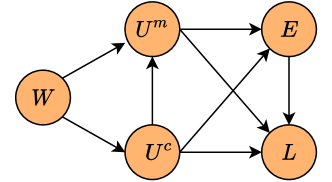
[Causal Dependency Graph of Performance Metrics for a Service Instance]This graph depicts the causal relationship between various performance metrics for an instance of a service. The root node represents the workload, and the leaf node represents latency.

Figure 2. Causal metric graph for each instance of a service.

Similar to a previous approach (Li et al., 2022), we define certain causal assumptions between the metric categories based on domain knowledge of system engineers to define a causal metric graph (Fig. 2). A workload request at a microservice in turn demands resource utilization within the microservice, while the latency is the final effect of the request and hence is the leaf node in the metric graph. Such an assumption holds for all the microservices and their instances.

For request delivery across microservices, we employ the assumption that holds for a generic microservice architecture, that is, the latency and error metrics of a service depend on the callee microservice, while the workload depends on the workload of the caller microservices. Concisely, for a request trace from microservice A to B, where B is the callee microservice and A is the caller microservice, the ground-truth interservice edges that we consider in our formulation are $W^{A}_{t}\rightarrow W^{B}_{t}$, $L^{B}_{t}\rightarrow L^{A}_{t}$, and $E^{B}_{t}\rightarrow E^{A}_{t}$. A causal metric graph with a different selection of metrics can be easily integrated through data-specific domain knowledge.

4.2. Preliminary Approaches

We describe two approaches and identify how they fail to capture the system state in the estimated dependency graph.

4.2.1. Instances as Dedicated Nodes

A naïve approach to model each instance of a service in the causal graph $\mathcal{G}$ is to have a dedicated node for each $x_{ij}$ representing a metric from each instance of a service $\mathcal{S}$. However, whether causal functions are distinct for each instance of $\mathcal{S}$ can be tested by running the hypothesis $f_{ij}=f_{i}$ $\forall j$, given enough data. But, due to the short-lived and ever-changing nature of instances being spawned, some instances might get killed and not be re-spawned again with identical physical characteristics. Hence, available metric data for some instances might be scarce and a stable relational function might not be obtained, making the solution infeasible. In addition, with the number of instances varying over time due to auto-scaler decisions, a dynamic causal graph might be needed if each node in the causal graph corresponds to an individual instance of a service. Moreover, the naïve solution incurs huge computation to run causal structure estimation with 1000’s of instances deployed per service in a large microservice ecosystem.

4.2.2. Value Aggregation across Instances

For each microservice $\mathcal{S}$, this approach (termed as Avg-fGES) groups relevant metrics that causally affect metrics in $\mathcal{S}$ to identify the causal structure of $\mathcal{S}$, i.e., all the five metrics for each instance of $\mathcal{S}$, along with the workload for all instances of caller services and latency and error metrics for all instances of callee services of $\mathcal{S}$ in the service call graph. However, the number of metric values for each service (which is equal to the number of instances) changes with time due to the changing number of instances. Hence at each time instant $t$, to consolidate the metric values for all the instances of a service $x_{ijt}\forall j$, Avg-fGES averages (other aggregation methods can be used) them across the number of instances to form a single aggregated metric $y_{it}$. Formally,

(2) $$y_{it}=\frac{1}{num\_inst(\mathcal{S})}\sum_{j=1}^{num\_inst(\mathcal{S})}x_{ijt}$$

Thus, using the aggregated metric values $y_{it}\forall i$ filtered for service $\mathcal{S}$ and running fGES yields the causal structure.

Why Aggregation Fails? Averaging the metric values across all instances for a service results in loss of information (Moghimi and Corley, 2020; Marvasti, 2010) and hence fails to capture the true dependency relationships among the metrics. A subset of instances of a service might suffer from high utilization periods, but averaging the metric values across all instances dilute the effect of certain instances (Fig. 3), and we lose critical dependencies for such instance exhibiting extreme behavior due to aggregation. Hence the causal relationships will not capture such extreme behaviors.

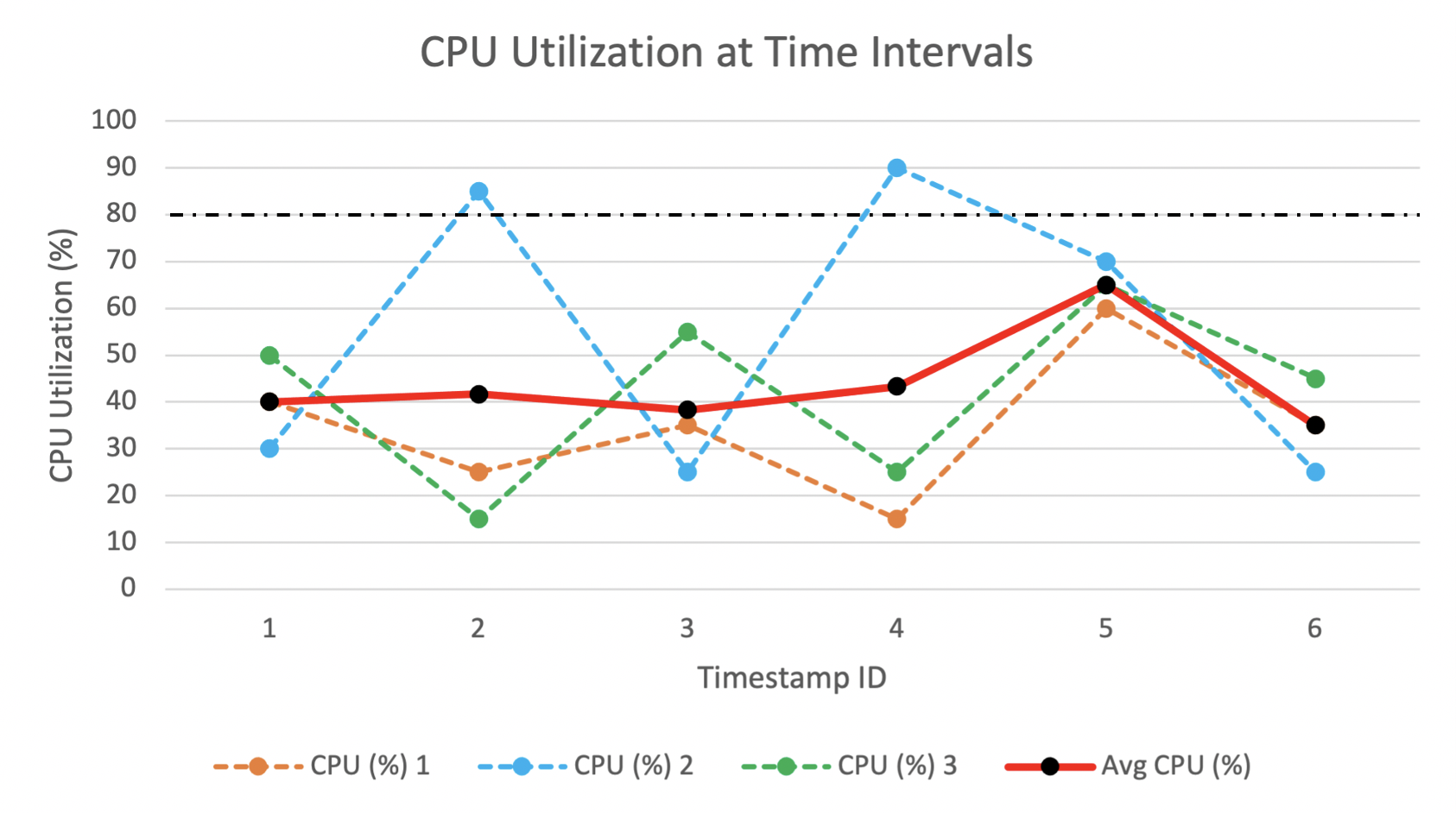
[Line chart showing variation of CPU Utilization]This chart depicts the variation of CPU Utilization for three instances and their average against timestamp and shows how averaging the metric values across all instances dilute the effect of the value of certain instances. Although CPU utilization of one instance is above a threshold, the average over 3 instances is below the threshold.

Figure 3. Variation of CPU Utilization against timestamp for 3 instances and their average CPU utilization.

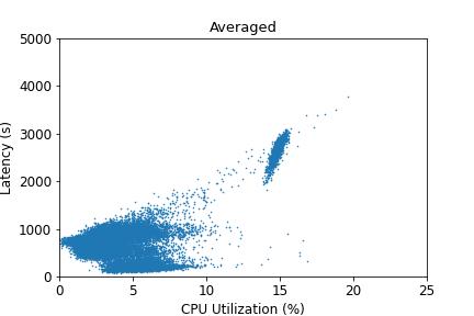
(a)

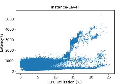
(b)

Figure 4. Averaging data across instances changes the relationship between two metrics. In (b), where metric value for each instance is plot, it shows a quadratic-type relationship between latency and cpu utilization, which gets distorted in (a) due to averaging.

[Scatter plot showing the relationship between latency and cpu utilization for average vs instance level data]In (a), average metric value for is plotted which shows distortion. In (b) metric value for each instance is plotted, and it shows a quadratic-type relationship between latency and cpu utilization. It shows how averaging data across instances changes the relationship between two metrics.

Furthermore, system metrics exhibit non-linear dependencies amongst themselves (Masouros et al., 2020), which get deformed when metric values are averaged (Fig. 4(b)). For example, as shown in Fig. 4(b) obtained from real data, latency shows a non-linear dependency with CPU utilization, with dependencies differing between high and low utilization periods. Consequently, CausIL models non-linear dependencies among the performance metrics at an instance level. Similar issues prevail for any aggregation metric (sum, max, percentile, etc.). Summing-up metrics like CPU-Usage might drown out signals from faulty instances on receiving noise from normal instances. For example, the CPU utilization of two instances increasing by 10% might be normal but one increasing by 20% while another staying same might be a fault signal, the difference not being captured by just summing up the utilization values.

4.3. CausIL: Proposed Approach

To alleviate the issues elicited in the above sections, we propose CausIL that models data observed in multiple instances for each service. We further describe how system domain knowledge can be used to improve accuracy of any causal graph learning algorithm.

4.3.1. Instances as IID Draws

To motivate the design of CausIL, we look at how Kubernetes or similar platforms deploy services where multiple instances (or pods) of a microservice are launched with the same configurations (k8h, 2022). Secondly, these containerized instances are isolated and mostly operate independently of each other (ibm, 2019), making them conditionally independent on upstream and downstream metrics like utilization and latency. Their deployment in general, guarantees that there is no interference from other instances of the same service due to co-location (goo, 2016). It can be safely inferred that conditioned on the load received at the service, its different instances are essentially independent and identical, which we use as an explicit assumption in modeling CausIL. In short, let $W_{j},U_{j}$ be the workload and CPU Usage for instance $j$ of a service respectively, then the conditional distribution $U_{j}|W_{j}$ is independent of $U_{k}|W_{k}$, whereas whereas $U_{j}$ and $U_{k}$ are almost certainly dependent.

During high-load requests, the auto-scalers scale up the number of instances for a particular service, and the load balancer distributes the load almost equally (as we observe from real data) to each of the instances. Performance metrics for an instance depend on the amount of load distributed to only that instance. Following our assumption of instances being conditionally independent given the workload, it implies that the causal function for each instance is the same. Hence, Eq. 1 can be rewritten as:

(3) $$x_{ijt}=f_{i}(\mathcal{P}(x_{ijt}))+\epsilon_{ijt}$$

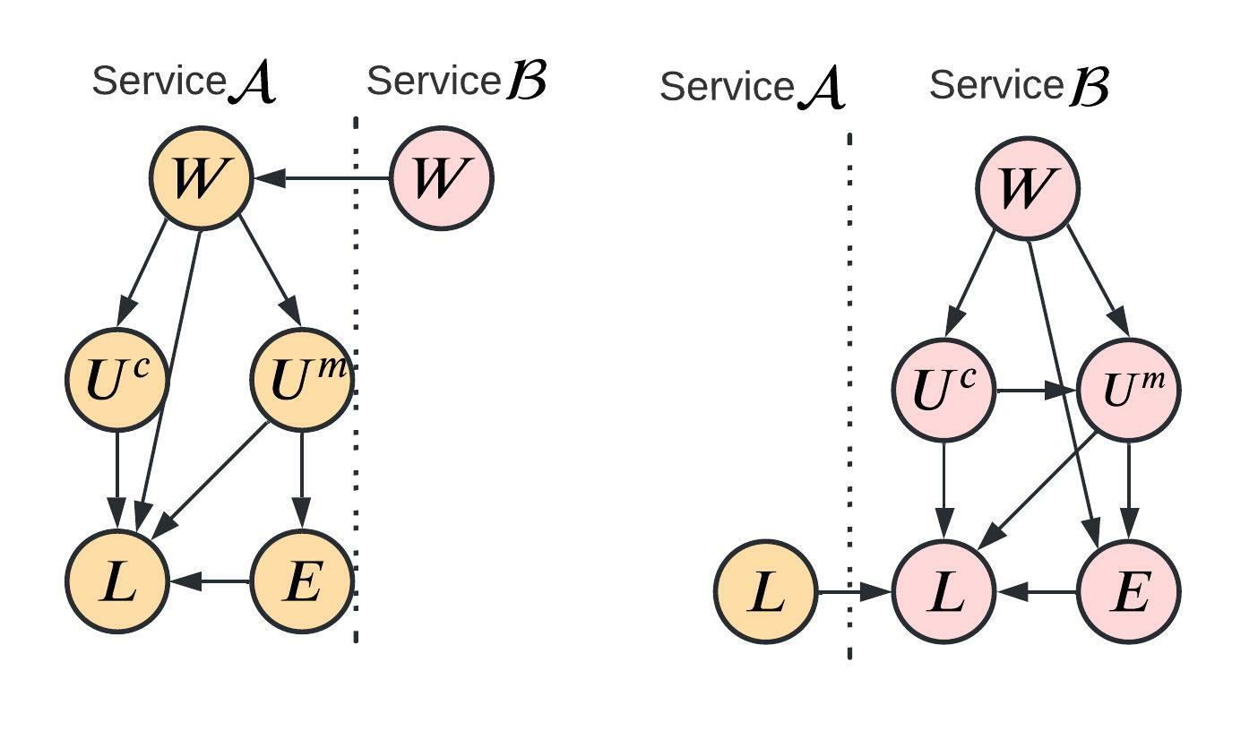
(a)

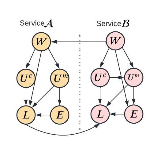
(b)

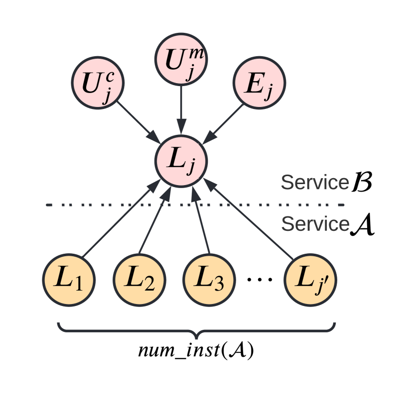
(c)

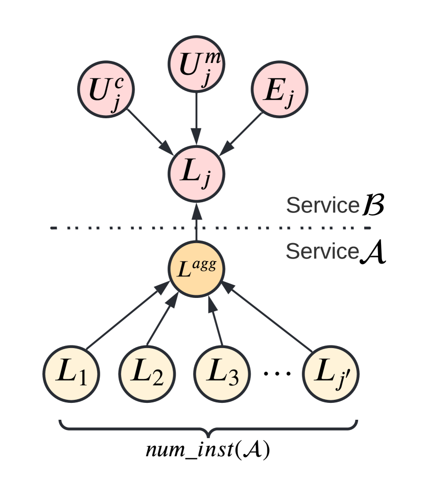
(d)

Figure 5. (a) shows an example estimated causal graph for individual services $\mathcal{A}$ and $\mathcal{B}$ where $\mathcal{B}$ calls $\mathcal{A}$. (b) shows the merged causal graph with error and workload merged. Figure (c) and (d) shows the parent metrics for latency of instance $j$ of $\mathcal{A}$. In (c) latency of $\mathcal{B}$ depends on metrics of $\mathcal{B}$ and latencies of all instances of $\mathcal{A}$. In (d) an aggregated latency node composed from the latencies of all instances of $\mathcal{A}$ is constructed, acting as a latent node.

[Examples of estimated causal graph for individual services A and B]Figure (a) depicts an example of an estimated causal graph for individual services A and B, where service B calls service A. Figure (b) shows the merged causal graph, where error and workload are combined. Figures (c) and (d) represent the parent metrics for the latency of instance j of service A. In (c), the latency of service B is dependent on the metrics of service B and the latencies of all instances of service A. In (d), an aggregated latency node is constructed from the latencies of all instances of service A, serving as a latent node.

4.3.2. Structure Estimation

Similar to Avg-fGES, CausIL identifies the causal structure between the metric nodes, as in §4.1, for one service at a time, making it highly scalable since its complexity will be linear in terms of the number of services. Causal structures of each microservice are then merged appropriately to form the final causal structure as shown in Fig. 5(b). Following the conditional independence assumption of the instances at time $t$, metrics for each instance of a service can be treated as an iid sample from a distribution, realized by flattening the data over the instances.

To reduce computation and improve accuracy while estimating the set of parents for a metric, CausIL selects relevant parent metrics from the concerned service $\mathcal{S}$ and its adjacent services $\mathcal{S}_{c}$ that causally affects some metrics of $\mathcal{S}$ before running fGES. For any metric $x_{ijt}$ of instance $j$ of service $\mathcal{S}$, viable parent metrics set include all the metrics from the same instance, the workload for all instances of caller services and latency and error metrics for all instances of callee services of $\mathcal{S}$. For example, latencies of all instances of callee service can affect the latency of an instance of their caller (Fig. 5(c)). Metrics for all the instances belonging to only the adjacent services are aggregated for each service as illustrated in Fig. 5(d). This is supported by our domain knowledge, since all instances of caller service can call an instance of callee service, which gets managed by the load balancer. Thus, the possible metric nodes that can exhibit dependencies with instance $j$ of $\mathcal{S}$ are all the metrics $\{x_{ijt}\},\forall i$, and union of the aggregation of all the metrics $i^{\prime}$ over all instances of adjacent $\mathcal{S}_{c}$ that causally affect $\mathcal{S}$ in the interservice edges of the call graph, or $\{x^{agg}_{i^{\prime}t}\}$.

After filtering the data for each microservice $\mathcal{S}$, CausIL discovers the causal structure between the nodes. We minimize the BIC-based score function of fGES, which is computed by running a regression model with $x_{ijt}$ data flattened across number of instances as the dependent variable and parent metrics $\mathcal{P}(x_{ijt})$ as the predictors. The score function is defined as

(4) $$\begin{split}Score(x_{ijt},\mathcal{P}(x_{ijt}))=&-2\sum_{j,t}\log\mathcal{(}L(f_{i}(\mathcal{P}(x_{ijt}))|x_{ijt},\mathcal{P}(x_{ijt})))\\ &+\rho k\log n_{i}\end{split}$$

where, $\rho$ is a penalty term that penalizes the estimation of an over-fitting function with large number of parameters, $k$ number of parameters in $f_{i}$, and $n_{i}$ is the number of observation after flattening the data. We found $\rho=2$ to be optimal for our experiments via hyperparameter tuning.

4.3.3. Structural Graph Post-Processing

CausIL generates a completed partially directed acyclic graph (CPDAG) comprising of directed as well as undirected edges. However, undirected edges render the causal graph infeasible to use for a downstream task like root cause analysis. Thus, we direct the undirected edges. To avoid cyclic dependency, we topologically sort the nodes and then assign the direction $n_{i}\rightarrow n_{j}$ where $i<j$ in topological ordering for the undirected edges. This prevents the cycles and results in a directed acyclic graph (DAG).

4.3.4. Algorithm Specifics

Input: Service Call Graph($G_{c}$), Metrics Data at instance level($\mathcal{D}$)

Output: Estimated Causal Graph

1

2Read Data $\mathcal{D}$

3 Read Service Call Graph $G_{c}$

4 $G_{out}\leftarrow null$

 // Iterate over each service

5 for each service $N$ do

6       $\mathcal{D}_{filtered}\leftarrow$Data for metrics of all instances of service $N$

7       $\mathcal{D}_{filtered}\leftarrow$Agg ‘latency’ and ‘error’ over all instances for all child services of $N$

8       $\mathcal{D}_{filtered}\leftarrow$Agg ‘workload’ over all instances for all parent services of $N$

9       Stack data $\mathcal{D}_{filtered}$

10       $G^{\prime}\leftarrow$ Run fGES on $\mathcal{D}_{filtered}$ with domain knowledge

11       Append $G^{\prime}$ to $G_{out}$

12      

13Connect inter-service edges in $G_{out}$

14 return $G_{out}$

Algorithm 1 Discover Causal Structure

Algorithm 1 presents the workflow of CausIL. Note that we take only latency and error metrics for the child nodes and workload metric for the parent nodes due to the relationship stated in §3.

If the total latency of a request is larger than the data collection granularity, past workloads can affect metrics at the current timestamp. However, we observe that latency of requests is much lower (¡100 ms) than the data collection granularity (15 min). Thus, past workloads on current system state is minimal and hence we do not consider the lags in metrics during structural graph construction.

4.4. Incorporating Domain Knowledge

Domain knowledge plays an important role in improving the performance of CausIL in terms of accuracy and computation time. System data and metric semantics provide several easy ways to generalize rules applicable to any microservice architecture without needing a system expert. We apply such rules to form a list of commonly prohibited edges. Nevertheless, any system expert can append to the domain knowledge already provided, which however can be time-consuming and hence we omit them in this paper. A prohibited edge list reduces the space-time complexity of the causal discovery algorithm and restricts the formation of unnecessary edges from system architecture point of view. We propose a list of rules based on Site Reliability Engineers’ (SREs) input to automate the prohibited edge generation process.

Based on expert advice over the metric categories defined in §3, we prohibit edges in the causal graph at a single service level such that: (i) No other metric within the same service for any instance can affect workload, it can be either an exogenous node or depend on the workload of caller service. (ii) latency cannot affect resource utilization. Furthermore, rules for prohibiting inter-service edges are: (i) Prohibit all edges between services if they are not connected in the call graph. (ii) Prohibit all edges between services that are connected except (a) Workload metric in the direction of the call graph and (b) Latency and Error metrics in the opposite direction of the call graph. This follows from the informed causal assumptions across microservices presented in §4.1. This list of prohibited edges for all the microservices serves as the domain knowledge to be introduced to the causal discovery algorithm.

5. Experimental Setup

In this section, we give a brief description of the setup, dataset characteristics and the metrics used for the evaluation of our model. We implemented CausIL in Python while adapted and optimized publicly available libraries (fges-py and tetrad) for running fGES. We have run CausIL on a system having Intel Xeon E5-2686 v4 2.3GHz CPU with 8 cores.

5.1. Baselines and Models

We compare our proposed strategy CausIL against various baselines defined below. The algorithms below were tested with and without the application of Domain Knowledge (DK), which will be indicated as yes/no in the evaluation tables.

1. FCI: Fast Causal Inference is a constraint-based algorithm algorithm (Spirtes et al., 2000) which provides guarantees in causal discovery in the presence of confounding variables. We use the version of FCI that averages data across all instances.

2. Avg-fGES: Implementation of the algorithm described in §4.2.2. Multiple estimation functions $f_{i}$ in Eq. 3 estimating the dependency score between parent metrics and the child metric have been implemented; (i) Avg-fGES-Lin: Ordinary Least Square $f_{i}$, (ii) Avg-fGES-Poly2: Polynomial $f_{i}$ of degree 2, (iii) Avg-fGES-Poly3: Polynomial $f_{i}$ of degree 3.

3. CausIL: Different versions of the proposed method has been implemented that varies in their estimation functions $f_{i}$;

   (i) CausIL-Lin: Ordinary Least Square $f_{i}$, (ii) CausIL-Poly2: Polynomial $f_{i}$ of degree 2, (iii) CausIL-Poly3: Polynomial $f_{i}$ of degree 3.

5.2. Datasets

We evaluated CausIL against a set of synthetic and semi-synthetic, while a case study on a real-world dataset is presented as well.

Synthetic ($\mathcal{D}^{syn}$): Three datasets are generated with 10/20/40 services and each service having 5 metric nodes, thus making a total of 50/100/200 nodes respectively in the causal graph. The metric nodes within and across the services were connected according to §4.1, and data was generated according to Alg. 3 in appendix, which accurately mimics the behavior of a load-balancer and auto-scaler in a real scenario. We present evaluations for each dataset by averaging across 5 graphs. For each instance of a service, time series dataset of a metric $\mathbf{x_{ijt}}=f_{i}(\mathcal{P}(\mathbf{x_{ijt}}))$ is generated, where $f$ is a non-linear quadratic function. Workload for a service $s$ ($W_{s}$) is distributed across each instance uniformly. Across adjacent services $a\rightarrow b$, $W_{b}=\beta W_{a}$, where $\beta\in[0,1]$.

Semi-Synthetic ($\mathcal{D}^{semi-syn}$): With the same graphs generated as in above, causal relationships across metrics are learnt based on data gathered from a real-world service. For each edge in Figure 2, we learn a random forest regressor and then generate output metric value with added random error given parent metric inputs to the function. The function learnt for a metric $x_{i}$ remains same for each instance and service. Workload for exogenous services is equal to the workload of real-world services.

5.3. Evaluation Metrics

Following existing works (Raghu et al., 2018), we evaluate the causal graph generated by CausIL using the following metrics.

1. Adjacency Metrics (Adj) denotes the correctness of the edges in the graph as estimated by CausIL by disregarding the directions of the edges.

2. Arrow Head Metrics (AH) considers the causal orientations of the edge when considered against the true graph and penalizes for the incorrectly identified directions of the correctly identified adjacencies.

3. Structural Hamming Distance (SHD) reports the number of changes that must be made to an estimated causal graph to recreate the ground truth graph.

We report precision (P), recall (R) and F1-score (F) with their usual semantics for Adjacency and Arrow Head metrics. While adjacency metric records precision/recall of identified edges and rewards correctly identified edges, SHD measures edit distance between two graphs and penalizes misidentified/missing edges

[Plots showing how domain knowledge helps in causal structure estimation]Fig. (a), (c) and (e) are bar plots showing the difference in SHD for the three datasets (10/20/40 services). The difference between the run with domain knowledge shows a significant decrease in the SHD than the one run without any domain knowledge. Also, the time taken to construct the graph shows 70x improvement with domain knowledge.

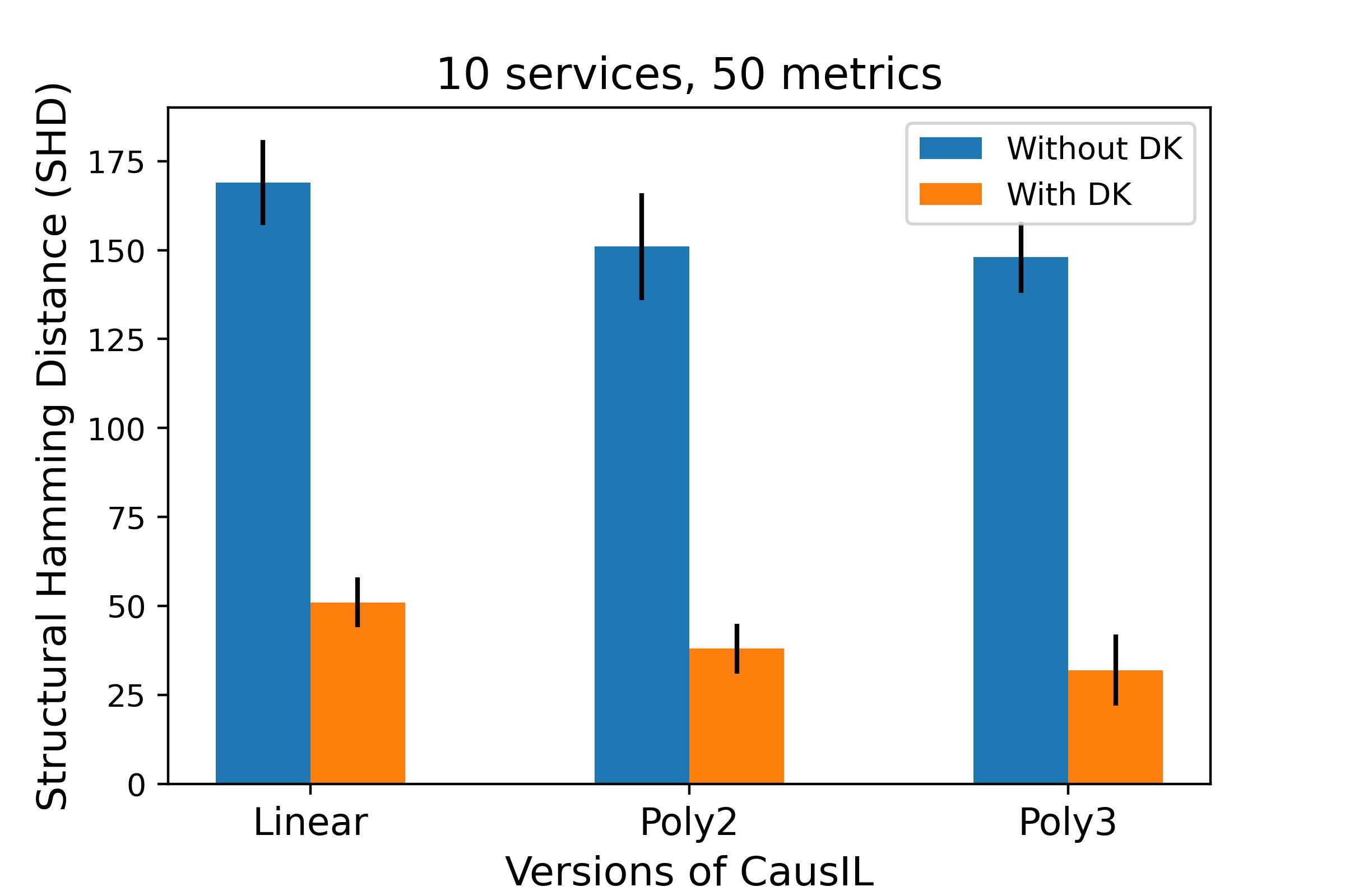
(a)

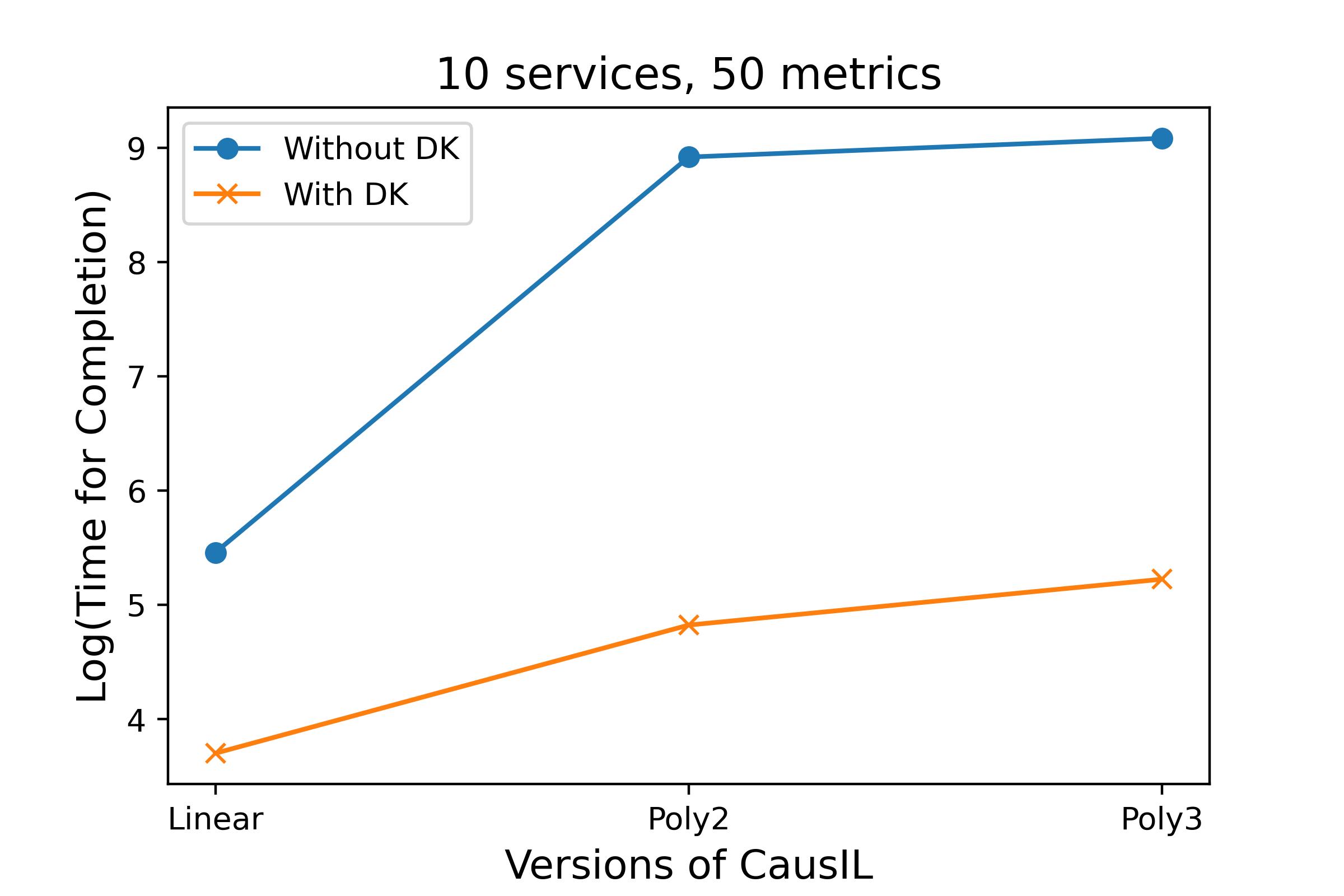
(b)

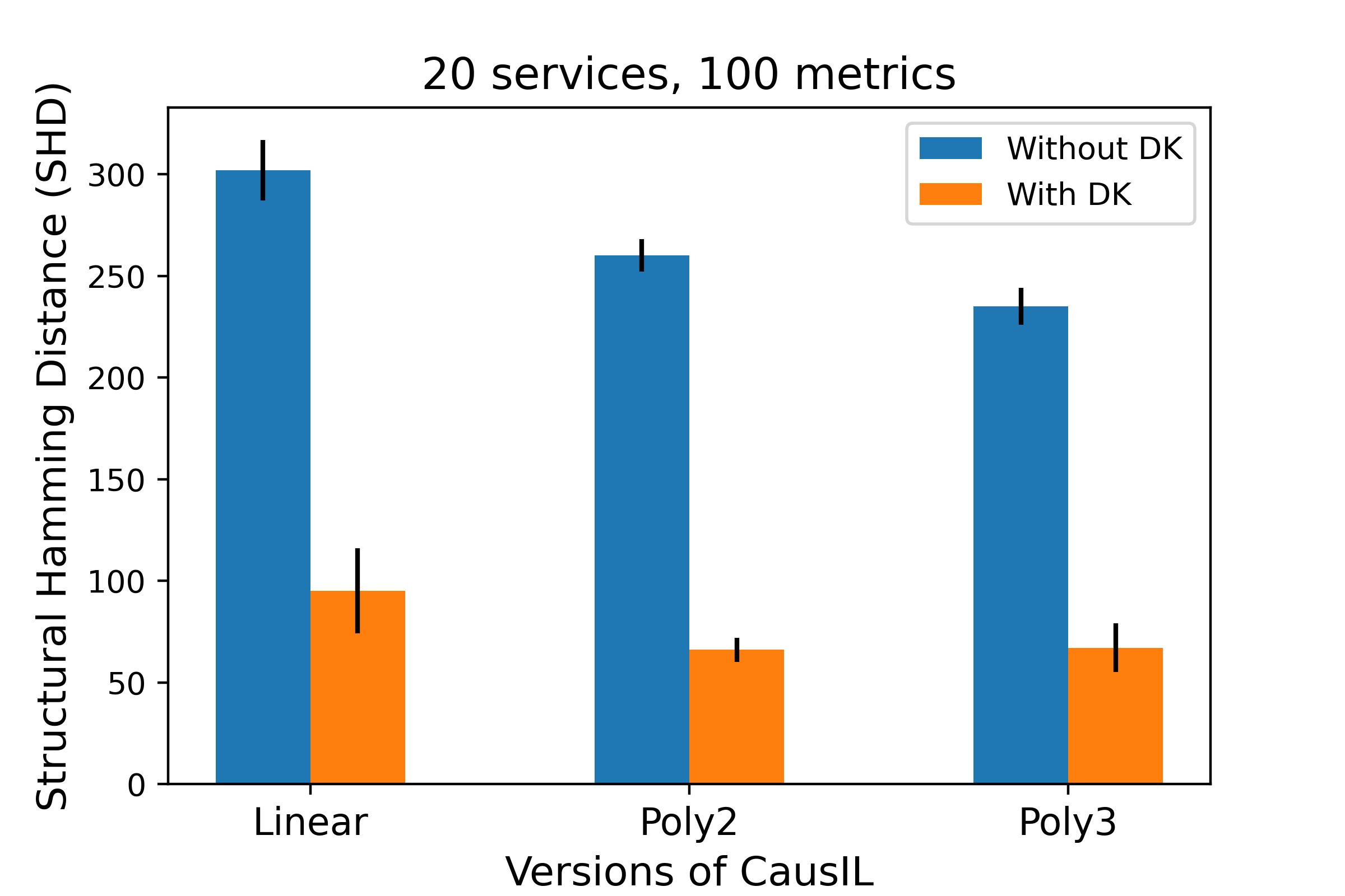
(c)

(d)

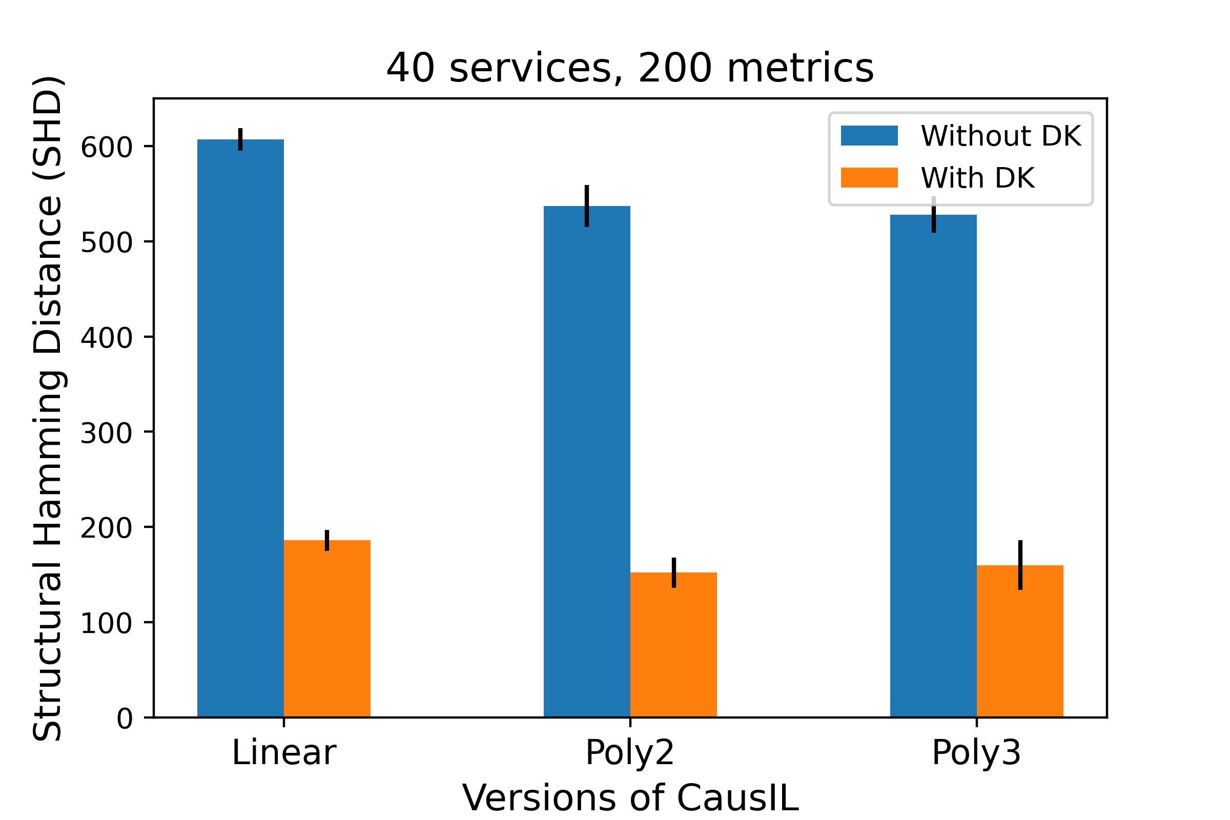
(e)

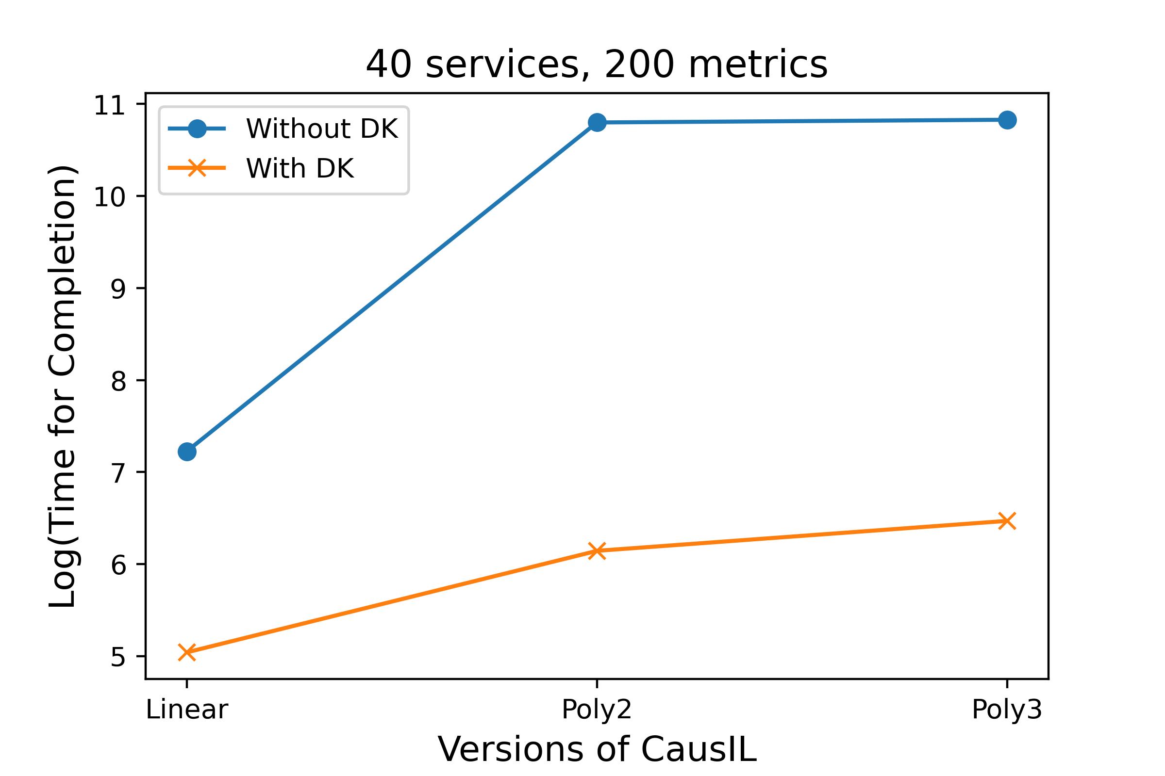
(f)

Figure 6. Demonstrating how domain knowledge (DK) helps in causal structure estimation. Fig. (a), (c) and (e) show the difference in SHD for the three datasets, while (b), (d) and (f) show the improvements in time (logarithmic scale).

6. Evaluation Results

This section presents the evaluations performed to demonstrate the effectiveness of CausIL against the various baselines.

6.1. Impact of Domain Knowledge

We state in §4.4 that the use of domain knowledge for the system architecture in the form of prohibited edge list greatly boosts the accuracy of CausIL. Additionally, it also reduces computational time and complexity. In this section, we elucidate this improvement in performance with synthetic data for different version of CausIL in Fig. 6. We only report SHD in this section since it can effectively penalize redundant edges estimated when CausIL is employed without domain knowledge. Thus it forms a more decisive metric than the others in evaluating the impact of domain knowledge in the construction of the causal graph.

Fig. 6 shows that using domain knowledge of the system architectures improves the SHD of the estimated causal graph by more than $3.5\times$ across all models. With domain knowledge restricting the formation of edges that violate system rules, CausIL can better understand the structure of the system metrics and keep only the relevant edges. It also reduces the time taken for CausIL to estimate the causal graph by more than $70\times$ because computing the causal dependency score and function estimation by the underlying fGES is not required for certain child-parent pairs. Also, because the dataset was generated using a non-linear function, the model version implementing the linear estimation function performs the worst for each dataset. The benefit of introducing domain knowledge can be observed across various scales of the dataset. We will report the results of the remaining evaluations when estimation involved domain knowledge.

6.2. Baseline Comparison

# Services, # Metrics	Model	$\mathcal{D}^{syn}$							$\mathcal{D}^{semi-syn}$
		SHD	AdjP	AdjR	AdjF	AHP	AHR	AHF	SHD	AdjP	AdjR	AdjF	AHP	AHR	AHF
10, 50	FCI	53	0.772	0.841	0.805	0.704	0.909	0.793	53	0.762	0.873	0.814	0.69	0.906	0.783
	Avg-fGES-Lin	54	0.794	0.854	0.822	0.686	0.864	0.765	54	0.793	0.851	0.82	0.68	0.857	0.759
	Avg-fGES-Poly2	48	0.81	0.861	0.834	0.723	0.892	0.799	50	0.807	0.845	0.825	0.713	0.883	0.789
	Avg-fGES-Poly3	46	0.837	0.839	0.837	0.747	0.893	0.814	46	0.837	0.838	0.836	0.745	0.89	0.811
	CausIL-Lin	51	0.788	0.878	0.83	0.695	0.882	0.777	53	0.788	0.874	0.829	0.684	0.868	0.765
	CausIL-Poly2	38	0.889	0.852	0.869	0.795	0.895	0.842	36	0.892	0.877	0.883	0.795	0.892	0.84
	CausIL-Poly3	32	0.909	0.878	0.891	0.823	0.905	0.862	35	0.909	0.875	0.89	0.797	0.877	0.835
20, 100	FCI	105	0.773	0.85	0.81	0.702	0.909	0.792	105	0.772	0.856	0.811	0.699	0.906	0.79
	Avg-fGES-Lin	103	0.814	0.832	0.82	0.706	0.867	0.778	104	0.813	0.827	0.818	0.709	0.872	0.782
	Avg-fGES-Poly2	95	0.823	0.872	0.847	0.716	0.87	0.786	93	0.826	0.886	0.855	0.713	0.864	0.781
	Avg-fGES-Poly3	88	0.845	0.867	0.857	0.74	0.876	0.802	85	0.846	0.871	0.836	0.782	0.869	0.798
	CausIL-Lin	95	0.812	0.856	0.832	0.728	0.897	0.803	100	0.809	0.836	0.82	0.722	0.892	0.797
	CausIL-Poly2	66	0.908	0.895	0.901	0.801	0.883	0.84	68	0.907	0.892	0.899	0.795	0.876	0.833
	CausIL-Poly3	67	0.913	0.881	0.896	0.807	0.884	0.844	72	0.911	0.859	0.884	0.804	0.882	0.841
40, 200	FCI	204	0.792	0.814	0.803	0.719	0.907	0.803	206	0.781	0.802	0.791	0.706	0.904	0.793
	Avg-fGES-Lin	203	0.837	0.78	0.807	0.742	0.886	0.808	206	0.837	0.778	0.806	0.737	0.88	0.802
	Avg-fGES-Poly2	197	0.853	0.782	0.815	0.749	0.879	0.809	200	0.852	0.779	0.813	0.746	0.876	0.806
	Avg-fGES-Poly3	204	0.862	0.741	0.795	0.763	0.886	0.82	203	0.862	0.746	0.799	0.759	0.882	0.816
	CausIL-Lin	186	0.835	0.811	0.824	0.759	0.897	0.827	188	0.833	0.811	0.822	0.755	0.905	0.823
	CausIL-Poly2	152	0.919	0.828	0.871	0.825	0.899	0.86	155	0.92	0.817	0.864	0.809	0.879	0.843
	CausIL-Poly3	160	0.922	0.783	0.846	0.83	0.909	0.863	162	0.922	0.784	0.847	0.821	0.89	0.854

[Table showing the comparison of CausIL against the baselines for all types of datasets.] It summarizes the performance of CausIL for synthetic and semi-synthetic data and demonstrates how preserving the instance-specific variations across various services helps and all estimation functions of CausIL outperform the baselines.

Table 1. Comparison of CausIL against the baselines for all types of datasets.

Table 1 summarizes the performance of CausIL for synthetic and semi-synthetic data and demonstrates how preserving the instance-specific variations across various services helps. The estimated causal graph is evaluated against the ground truth causal graph constructed during data generation, and thus, CausIL aims to implicitly learn the data generation process.

We observe from Table 1 that all estimation functions of CausIL outperform their corresponding versions of Avg-fGES by $\sim 25\%$ on average. CausIL captures more granular information about the system structure and how instance-specific variation of each metric causally affects other metrics. Thus, the causal graph learned by CausIL is more accurate than the baselines when compared against ground-truth (more correctly identified edges and fewer missing edges). We demonstrate this using a toy example (§A.1), where Avg-fGES could not discover (cpu utilization, latency) and (memory, error) edges, which CausIL predicted. Qualitatively, for downstream tasks like root cause detection, inaccurate graph estimated by the baselines can lead to incorrect conclusions about faulty service if graph traversal algorithms (Chen et al., 2014) are used, which a graph estimated by CausIL can limit.

Furthermore, for each of the baseline categories, the one implementing the non-linear estimation function provides better metric values than the linear counterpart. With data being generated from a non-linear function, it is intuitive that a linear estimation function won’t be able to capture the relationships succinctly. With increase in the degree of non-linearity in estimation function, CausIL shows a general trend in performance. We have implemented multiple versions of polynomial estimation functions $f_{i}$ differing in their degree. However, a score-based approach (BIC) can also guide the function choice. CausIL also outperforms FCI in SHD. We notice that arrow head recall for FCI is more than CausIL, though precision is less. This implies that FCI generates a causal graph with a large number of directed edges as compared to ground truth, trying to estimate a denser graph. In terms of memory overhead, CausIL incurs  100MB more than baseline on average.

We further observe that CausIL with synthetic data outperforms when run on semi-synthetic data for the same graph and the same model. This is because semi-synthetic data have correlated and dependent values among various exogenous nodes as well as maintain autoregressive nature of the time series, which makes it intrinsically harder for an algorithm to establish causal dependencies.

6.3. Real-World Use Case Study

We further evaluate CausIL against a real-world dataset collected from a part of a production-based microservice system of an enterprise cloud-service. The call graph for the system follows a star-shaped architecture with a total of 1 monolith calling 9 microservices (§B). The data was collected from Grafana, a monitoring tool that tracks and logs the metric values of several components of a running system at certain time intervals. We collected data for a span of 2 months with 5 minutes granularity.

With the unavailability of a ground truth causal graph between performance metrics for real data, we construct it based on the causal assumptions stated in §4.1 and then evaluate the estimated causal graph against it. We observe from Table 2 that CausIL-Poly2 performs the best among the other models. Though versions of Avg-fGES have high adjacency values, that is, they can estimate edges between the metrics, but the direction of the edges suffers, which is evident from their low arrow head metrics. FCI also performs poorly with real data. Each of the models on average estimates 25-30 undirected edges out of possible 113 ground truth edges.

Model	SHD	AdjP	AdjR	AdjF	AHP	AHR	AHF
FCI	59	0.756	0.796	0.775	0.697	0.922	0.794
Avg-fGES-Lin	52	0.829	0.858	0.843	0.692	0.835	0.757
Avg-fGES-Poly2	53	0.823	0.823	0.823	0.708	0.86	0.777
Avg-fGES-Poly3	51	0.852	0.814	0.833	0.722	0.848	0.78
CausIL-Lin	50	0.807	0.814	0.81	0.737	0.913	0.816
CausIL-Poly2	40	0.818	0.876	0.846	0.785	0.96	0.864
CausIL-Poly3	46	0.824	0.867	0.845	0.739	0.898	0.811

[Table showing the results of experiments on real data]Comparison shows that CausIL-Poly2 performs the best among the other models when run on real data

Table 2. Experiments on Real Data

7. Discussion

Scalability: CausIL discovers service-specific causal structures and then combines them to form the entire causal graph. Adding a new microservice will scale the computation time linearly. Based on the experiments using CausIL-Poly2 on multiple datasets, the average time for causal discovery for each service is 12-13s, with a standard deviation of 1.09s. Furthermore, parallelizing the discovery for each microservice would further improve the computation time.

Domain Knowledge: Aggregating minimal domain knowledge is not expensive since the edge exclusion list that CausIL uses is based on generic system architecture rules and principles. However, system engineers can decide to modify the rules as well, which might be expensive but not necessary, hence not compromising the estimation accuracy. Though argued to be a bad architectural design (Taibi et al., 2020), some real systems might also exhibit cyclic dependencies (Luo et al., 2021), making it hard to model. However, even in the presence of circular requests, microservice operations differ either in terms of multiple regional placements or distinct components are invoked. In such cases, we can essentially split it up into sub-services performing individual operations which can easily be handled by CausIL. On the contrary, circular dependency on services having identical operations will lead to an infinite loop and hence is not observed in real systems.

8. Conclusion

In this paper, we present a novel causal structure detection methodology CausIL that leverages metric variations from all the instances deployed per microservice. It makes a practical assumption based on system domain knowledge that the multiple instances of a service are identical and independent to each other conditioned on the load request received. Thus, CausIL filters relevant system metrics and models the causal graph at the metric-level using instance-level data variations. It estimates a causal graph for each microservice individually and then aggregates them over all microservices to form the final graph. An added advantage is its capability to cope with instances’ distinct and transitional nature, usually observed in a microservice deployment due to auto-scaler configuration.

We further show that incorporating system domain knowledge improves causal structure detection in terms of accuracy and computation time. It helps in estimating the essential edges and ignoring the non-existential edges. From our evaluations on simulated data, we show that our method outperforms the baselines by $\sim 25\%$, and the introduction of domain knowledge improves SHD by $\sim 3.5\times$ on average. We also evaluate on real data elucidating the practical usefulness of CausIL.

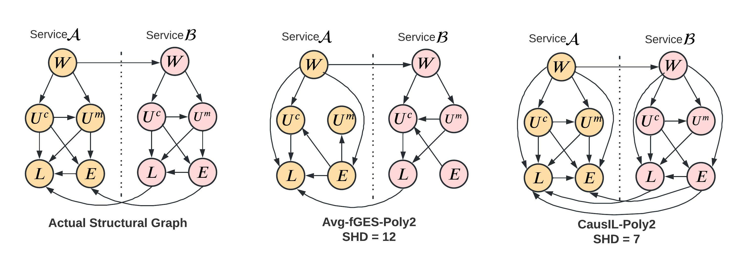
[Example on a dummy setup to show the benefit of CausIL]Example shows that the estimated causal graph from CausIL is able to identify more edges correctly as compared to the Avg-fGES on a 2 service dummy setup.

Figure 7. Illustration of the benefits of CausIL on a toy graph.

Appendix A Additional Evaluations

A.1. Illustration on Toy Graph

We illustrate why CausIL works better than the baseline via an example of a small toy call graph (Figure 7). We consider two services $A$ and $B$, such that $A$ calls $B$ ($A\rightarrow B$). For each of the service, we generate synthetic data (§5.2) for the metrics categories listed in §4.1 and create a ground truth causal graph following the causal assumptions. We run CausIL-Poly2 and Avg-fGES-Poly2 with domain knowledge on the synthetically generated data and report our findings here.

We observe that the Structural Hamming Distance for the estimated causal graph with CausIL is lower than the one estimated with the baseline method. Furthermore, some edges were not identified by Avg-fGES, which was identified by CausIL. This is because of the non-linearity in the dataset is reduced when the corresponding metrics for multiple instances are averaged. It does not capture the true distirbution of the data generation process. An evident example for this is the edge from memory utilization to latency for service $A$, which has been identified by CausIL, but Avg-fGES misses it. The adjacency and arrow head F1 score for CausIL are 0.857 and 0.774 respectively, while the same for Avg-fGES are 0.645 and 0.636 respectively, furthering bolstering the efficacy of CausIL.

A.2. Comparison against multiple aggregation function-based baselines

In §6.2, we have evaluated and compared CausIL against Avg-fGES, which aggregates a particular metric values for all the instances running for a service at any time $t$ by averaging them. However, though we argue that any aggregation function like summation, maximum etc. will have the same shortcoming as doing averaging where the entire spectrum of the relationship will not be captured, we empirically show this in Table 3.

We have evaluated on the synthetic dataset generated at multiple scales, that is, with 50 metric nodes, 100 metric nodes and 200 metric nodes. We report SHD, adjacency F1 score and Arrow Head F1 score. The baselines that we have evaluated against are:

1. Avg-fGES, where metric values over all instances are averaged at any particular time $t$

2. Max-fGES, where the maximum metric value over all the instances is taken at any time instant $t$

3. Min-fGES, where the minimum metric value is chosen

4. Sum-fGES, where metric values for all the instances are summed at any time instant $t$

We observe that CausIL outperforms all the baselines with Avg-fGES and Sum-fGES being the better performing baselines. This proves our claim empirically and the need for the design of a causal structure estimation method that takes into account instance specific variations.

# Services, # Metrics	Estimation Function	Avg-fGES			Max-fGES			Min-fGES			Sum-fGES			CausIL
		SHD	AdjF	AHF	SHD	AdjF	AHF	SHD	AdjF	AHF	SHD	AdjF	AHF	SHD	AdjF	AHF
10, 50	Linear	54	0.822	0.765	53	0.832	0.749	56	0.796	0.779	53	0.804	0.79	51	0.83	0.777
	Poly2	48	0.834	0.799	53	0.824	0.765	53	0.813	0.778	50	0.822	0.8	38	0.869	0.842
	Poly3	46	0.837	0.814	56	0.797	0.776	50	0.801	0.817	47	0.825	0.821	32	0.891	0.862
20, 100	Linear	103	0.82	0.778	98	0.834	0.785	109	0.807	0.775	101	0.816	0.801	95	0.832	0.803
	Poly2	95	0.847	0.786	97	0.827	0.802	99	0.822	0.801	89	0.853	0.799	66	0.901	0.84
	Poly3	88	0.857	0.802	106	0.813	0.778	106	0.797	0.801	86	0.847	0.825	67	0.896	0.844
40, 200	Linear	203	0.807	0.808	204	0.802	0.812	229	0.765	0.802	211	0.791	0.812	186	0.824	0.827
	Poly2	197	0.815	0.809	211	0.789	0.813	228	0.76	0.809	205	0.807	0.802	152	0.861	0.86
	Poly3	204	0.795	0.82	214	0.777	0.821	224	0.757	0.823	204	0.803	0.808	160	0.846	0.863

[Table showing the results of experiments based on different aggregation function]Comparison shows that CausIL outperforms all the versions of instance level data aggregation schemes like Avg-fGES, Sum-fGES, Max-fGES and Min-fGES.

Table 3. Comparison of CausIL against multiple baselines. Avg-fGES averages the metric values over all instances for each time instant. Similarly, Max-fGES computes the maximum, Min-fGES computes the minimum and Sum-fGES computes the sum of the metric values over all instances for any time $t$.

Appendix B Real Graph Details

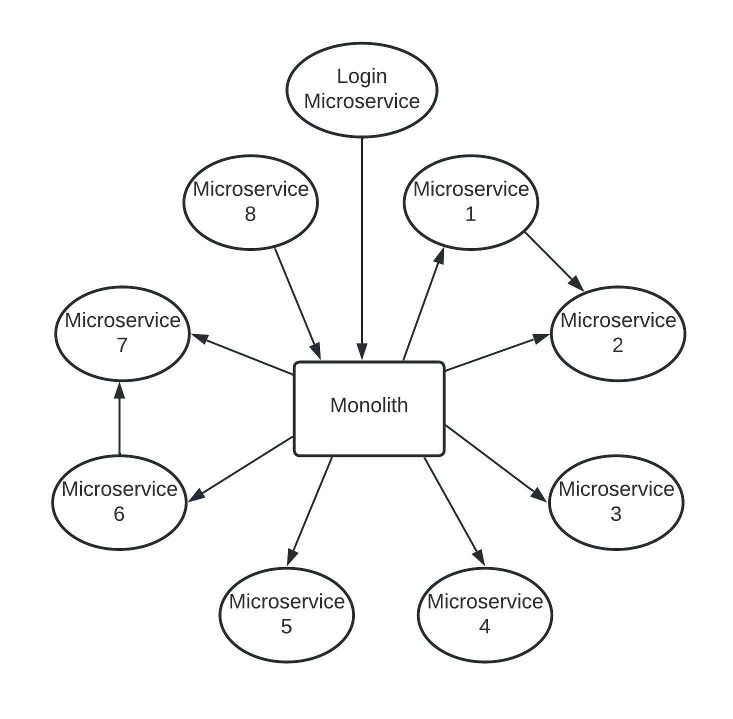
[Service Call Graph for real data]Total of 9 microservices in a star schema where the monolith calls 8 microservices and 1 microservice calls the monolith. Apart from these, microservice 1 also calls microservice 2, and microservice 6 calls microservice 7.

Figure 8. Service Call Graph for real data

In our study with the real data, the underlying service architecture from which the data was collected is illustrated in Figure 8. We collect metrics for each service belonging to the metric categories defined in §4.1, and construct a causal structural graph against which we evaluate. Though, ground truth graph is unknown in a real world setting, we use our constructed graph as a proxy for the ground truth.

Appendix C Data Generation

From a given structural graph, we generate synthetic and semi-synthetic data. We construct a directed acyclic graph of services (call graph) and use it to generate a ground truth causal graph at the metrics level, following existing work (Zheng et al., 2018). The data is generated by using the edges between performance metrics for each service. Algorithm 2 is used to generate a random graph between services, which is then trivially extended to form the graph between performance metrics using the causal assumptions and rules described in §4.1.

Input: Number of nodes $N_{n}$, Number of edges $N_{e}$

Output: Service Call Graph $\mathcal{G}(N_{n},N_{e})$

1

2Initialize $\mathcal{G}(V,E)$, where $V=\{1,2,\ldots,N_{n}\},E=\phi$

3

4for $i\in\{2,3,\ldots,N_{n}\}$ do

5       $j\leftarrow$ sample a node from $\{1,2,\ldots,i-1\}$ randomly

6       $E\leftarrow E\cup\{(i\rightarrow j)\}$

7      

8for $k\in\{N_{n},\ldots,N_{e}\}$ do

9       $i\leftarrow$ sample a node from $\{2,3,\ldots,N_{n}\}$

10       $j\leftarrow$ sample a node from $\{1,2,\ldots,i-1\}$

11       if $(i\rightarrow j)\notin E$ then

12             $E\leftarrow E\cup\{(i\rightarrow j)\}$

13            

14      

return $\mathcal{G}$

Algorithm 2 Generate Random Graph

Input: Real Data $\mathcal{D}_{real}$, Service Call Graph $\mathcal{G}$

Output: Synthetic/Semi-Synthetic Data $\mathcal{D}$

1

2for each dependency edge $i$ in Figure 2 do

3       Generate quadratic/Learn function $f_{i}$

4      

Learn function $f_{0}:W^{agg}\rightarrow R$

 // $R=$ # instances

5

6$\mathcal{D}_{exog}\leftarrow$ random distribution /$\mathcal{D}_{real}[W^{agg}]$

7

8for $t=1,2,\ldots$ do

9       for service $i$ do

10             if $i$ = exogenous service then

11                   $W^{i,agg}_{t}\leftarrow\mathcal{D}_{exog}^{t}$

12                  

13             else

14                   $W^{i,agg}_{t}\leftarrow\sum_{j\in\mathcal{P}(i)}\beta_{j,i}*W^{j,agg}_{t}$

15                  

16            

17            Compute $R_{t}$ using $f_{0}$

18             For each instance $j$, $W_{ijt}\leftarrow N(\mu=\frac{W^{i,agg}_{t}}{R_{t}},\sigma=\frac{\mu}{10})$

19            

20            Compute CPU and Mem. Util. of $i$ based on $f_{i}+\epsilon$

21            

22            if $i$ is leaf node then

23                   compute Latency and Error based on $f_{i}+\epsilon$

24                   Recurse back

25            

26            for $k\in$ child($i$) do

27                   Goto Step 6 for service $k$

28                  

29            

30            if all child($i$) is computed then

31                   Compute $L^{agg}$ and $E^{agg}$ for each child($i$)

32                   Assign Latency and Error based on $f_{i}+\epsilon$

33                  

34            

35      

$\mathcal{D}\leftarrow$ all data generated for each service return $\mathcal{D}$

Algorithm 3 Generate Synthetic/Semi-synthetic Data

Algorithm 3 shows the steps required to generate synthetic or semi-synthetic data for a given call graph $\mathcal{G}$. We first create workload metric values for the exogenous nodes, that is, the nodes without any parent metrics. Workload for the service is distributed to its instances almost equally (Mean being total workload over number of instances). This is based on the observation from the real data where workload at instances were almost equal. Cpu and memory utilization values were computed based on the learned/generated functions, and then the metrics for the child services were computed similarly in a recursive nature. It is to be noted that we add a random gaussian error to the values of the metrics to avoid deterministic relationship of metric values across services.

References

- (1)
- net (2015) 2015. Why You Can’t Talk About Microservices Without Mentioning Netflix. https://smartbear.com/blog/why-you-cant-talk-about-microservices-without-ment/. (2015).
- goo (2016) 2016. Borg, Omega, and Kubernetes https://queue.acm.org/detail.cfm?id=2898444. (2016).
- ibm (2019) 2019. Application containerization https://www.ibm.com/in-en/cloud/learn/containerization/. (2019).
- new (2019) 2019. Caring for Container-Based Services with Checks, Monitoring, and Alerts. https://newrelic.com/blog/how-to-relic/container-service-checks. (2019).
- ube (2021) 2021. CRISP: Critical Path Analysis for Microservice Architectures. https://eng.uber.com/crisp-critical-path-analysis-for-microservice-architectures/. (2021).
- k8h (2022) 2022. Horizontal Pod Autoscaling https://kubernetes.io/docs/tasks/run-application/horizontal-pod-autoscale/. (2022).
- pod (2022) 2022. Pods. https://kubernetes.io/docs/concepts/workloads/pods/. (2022).
- Balalaie et al. (2016) Armin Balalaie, Abbas Heydarnoori, and Pooyan Jamshidi. 2016. Microservices architecture enables devops: Migration to a cloud-native architecture. Ieee Software 33, 3 (2016), 42–52.
- Beyer et al. (2016) Betsy Beyer, Chris Jones, Jennifer Petoff, and Niall Richard Murphy. 2016. Site Reliability Engineering: How Google Runs Production Systems (1st ed.). O’Reilly Media, Inc.
- Brandón et al. (2020) Álvaro Brandón, Marc Solé, Alberto Huélamo, David Solans, María S Pérez, and Victor Muntés-Mulero. 2020. Graph-based root cause analysis for service-oriented and microservice architectures. Journal of Systems and Software 159 (2020), 110432.
- Chen et al. (2014) Pengfei Chen, Yong Qi, Pengfei Zheng, and Di Hou. 2014. Causeinfer: Automatic and distributed performance diagnosis with hierarchical causality graph in large distributed systems. In IEEE INFOCOM 2014-IEEE Conference on Computer Communications. IEEE, 1887–1895.
- Chen et al. (2019) Yujun Chen, Xian Yang, Qingwei Lin, Hongyu Zhang, Feng Gao, Zhangwei Xu, Yingnong Dang, Dongmei Zhang, Hang Dong, Yong Xu, et al. 2019. Outage prediction and diagnosis for cloud service systems. In The World Wide Web Conference. 2659–2665.
- Chickering (2002) David Maxwell Chickering. 2002. Learning equivalence classes of Bayesian-network structures. The Journal of Machine Learning Research 2 (2002), 445–498.
- Coburn Watson and Gregg (2022) Scott Emmons Coburn Watson and Brendan Gregg. 2022. A Microscope on Microservices netflixtechblog.com/a-microscope-on-microservices-923b906103f4/. Netflix Technology Blog (2022).
- Gan et al. (2021) Yu Gan, Mingyu Liang, Sundar Dev, David Lo, and Christina Delimitrou. 2021. Sage: practical and scalable ML-driven performance debugging in microservices. In Proceedings of the 26th ACM International Conference on Architectural Support for Programming Languages and Operating Systems. 135–151.
- Hu et al. (2018) Jianpeng Hu, Linpeng Huang, Tianqi Sun, Yuchang Xu, and Xiaolong Gong. 2018. Log2Sim: automating what-if modeling and prediction for bandwidth management of cloud hosted Web services. In 2018 IEEE International Conference on Web Services (ICWS). IEEE, 99–106.
- Ikram et al. (2022) Muhammad Azam Ikram, Sarthak Chakraborty, Subrata Mitra, Shiv Saini, Saurabh Bagchi, and Murat Kocaoglu. 2022. Root Cause Analysis of Failures in Microservices through Causal Discovery. In Advances in Neural Information Processing Systems. https://openreview.net/forum?id=weoLjoYFvXY
- Jiang et al. (2016) Yurong Jiang, Lenin Ravindranath Sivalingam, Suman Nath, and Ramesh Govindan. 2016. WebPerf: Evaluating what-if scenarios for cloud-hosted web applications. In Proceedings of the 2016 ACM SIGCOMM Conference. 258–271.
- Laguna et al. (2013) Ignacio Laguna, Subrata Mitra, Fahad A Arshad, Nawanol Theera-Ampornpunt, Zongyang Zhu, Saurabh Bagchi, Samuel P Midkiff, Mike Kistler, and Ahmed Gheith. 2013. Automatic problem localization via multi-dimensional metric profiling. In 2013 IEEE 32nd International Symposium on Reliable Distributed Systems. IEEE, 121–132.
- Li et al. (2022) Mingjie Li, Zeyan Li, Kanglin Yin, Xiaohui Nie, Wenchi Zhang, Kaixin Sui, and Dan Pei. 2022. Causal Inference-Based Root Cause Analysis for Online Service Systems with Intervention Recognition. In Proceedings of the 28th ACM SIGKDD Conference on Knowledge Discovery and Data Mining. 3230–3240.
- Li et al. (2020) Ze Li, Qian Cheng, Ken Hsieh, Yingnong Dang, Peng Huang, Pankaj Singh, Xinsheng Yang, Qingwei Lin, Youjiang Wu, Sebastien Levy, et al. 2020. Gandalf: An intelligent, end-to-end analytics service for safe deployment in large-scale cloud infrastructure. In 17th USENIX Symposium on Networked Systems Design and Implementation (NSDI 20). 389–402.
- Liu et al. (2021) Dewei Liu, Chuan He, Xin Peng, Fan Lin, Chenxi Zhang, Shengfang Gong, Ziang Li, Jiayu Ou, and Zheshun Wu. 2021. Microhecl: High-efficient root cause localization in large-scale microservice systems. In 2021 IEEE/ACM 43rd International Conference on Software Engineering: Software Engineering in Practice (ICSE-SEIP). IEEE, 338–347.
- Luo et al. (2021) Shutian Luo, Huanle Xu, Chengzhi Lu, Kejiang Ye, Guoyao Xu, Liping Zhang, Yu Ding, Jian He, and Chengzhong Xu. 2021. Characterizing microservice dependency and performance: Alibaba trace analysis. In Proceedings of the ACM Symposium on Cloud Computing. 412–426.
- Marvasti (2010) MA Marvasti. 2010. Quantifying information loss through data aggregation. VMware Technical White Paper (2010), 1–14.
- Masouros et al. (2020) Dimosthenis Masouros, Sotirios Xydis, and Dimitrios Soudris. 2020. Rusty: Runtime interference-aware predictive monitoring for modern multi-tenant systems. IEEE Transactions on Parallel and Distributed Systems 32, 1 (2020), 184–198.
- Meek (1997) Christopher Meek. 1997. Graphical Models: Selecting causal and statistical models. Ph. D. Dissertation. PhD thesis, Carnegie Mellon University.
- Meng et al. (2020) Yuan Meng, Shenglin Zhang, Yongqian Sun, Ruru Zhang, Zhilong Hu, Yiyin Zhang, Chenyang Jia, Zhaogang Wang, and Dan Pei. 2020. Localizing failure root causes in a microservice through causality inference. In 2020 IEEE/ACM 28th International Symposium on Quality of Service (IWQoS). IEEE, 1–10.
- Moghimi and Corley (2020) Maryam Moghimi and Herbert W Corley. 2020. Information Loss Due to the Data Reduction of Sample Data from Discrete Distributions. Data 5, 3 (2020), 84.
- Mondal et al. (2021) Shanka Subhra Mondal, Nikhil Sheoran, and Subrata Mitra. 2021. Scheduling of Time-Varying Workloads Using Reinforcement Learning. In Proceedings of the AAAI Conference on Artificial Intelligence, Vol. 35. 9000–9008.
- Nadareishvili et al. (2016) Irakli Nadareishvili, Ronnie Mitra, Matt McLarty, and Mike Amundsen. 2016. Microservice architecture: aligning principles, practices, and culture. ” O’Reilly Media, Inc.”.
- Newman (2021) Sam Newman. 2021. Building microservices. ” O’Reilly Media, Inc.”.
- Nguyen et al. (2013) Hiep Nguyen, Zhiming Shen, Yongmin Tan, and Xiaohui Gu. 2013. Fchain: Toward black-box online fault localization for cloud systems. In 2013 IEEE 33rd International Conference on Distributed Computing Systems. IEEE, 21–30.
- Nguyen et al. (2011) Hiep Nguyen, Yongmin Tan, and Xiaohui Gu. 2011. Pal: P ropagation-aware a nomaly l ocalization for cloud hosted distributed applications. In Managing Large-scale Systems via the Analysis of System Logs and the Application of Machine Learning Techniques. 1–8.
- Pearl et al. (2000) Judea Pearl et al. 2000. Models, reasoning and inference. Cambridge, UK: CambridgeUniversityPress 19, 2 (2000).
- Qiu et al. (2020) Juan Qiu, Qingfeng Du, Kanglin Yin, Shuang-Li Zhang, and Chongshu Qian. 2020. A causality mining and knowledge graph based method of root cause diagnosis for performance anomaly in cloud applications. Applied Sciences 10, 6 (2020), 2166.
- Raghu et al. (2018) Vineet K Raghu, Allen Poon, and Panayiotis V Benos. 2018. Evaluation of causal structure learning methods on mixed data types. In Proceedings of 2018 ACM SIGKDD Workshop on Causal Discovery. PMLR, 48–65.
- Ramsey et al. (2017) Joseph Ramsey, Madelyn Glymour, Ruben Sanchez-Romero, and Clark Glymour. 2017. A million variables and more: the Fast Greedy Equivalence Search algorithm for learning high-dimensional graphical causal models, with an application to functional magnetic resonance images. International journal of data science and analytics 3, 2 (2017), 121–129.
- Schwarz (1978) Gideon Schwarz. 1978. Estimating the dimension of a model. The annals of statistics (1978), 461–464.
- Spirtes et al. (2000) Peter Spirtes, Clark N Glymour, Richard Scheines, and David Heckerman. 2000. Causation, prediction, and search. MIT press.
- Taibi et al. (2020) Davide Taibi, Valentina Lenarduzzi, and Claus Pahl. 2020. Microservices anti-patterns: A taxonomy. In Microservices. Springer, 111–128.
- Tariq et al. (2008) Mukarram Tariq, Amgad Zeitoun, Vytautas Valancius, Nick Feamster, and Mostafa Ammar. 2008. Answering what-if deployment and configuration questions with wise. In Proceedings of the ACM SIGCOMM 2008 conference on Data communication. 99–110.
- Tariq et al. (2013) Mukarram Bin Tariq, Kaushik Bhandankar, Vytautas Valancius, Amgad Zeitoun, Nick Feamster, and Mostafa Ammar. 2013. Answering “what-if” deployment and configuration questions with WISE: Techniques and deployment experience. IEEE/ACM Transactions on Networking 21, 1 (2013), 1–13.
- Thalheim et al. (2017) Jörg Thalheim, Antonio Rodrigues, Istemi Ekin Akkus, Pramod Bhatotia, Ruichuan Chen, Bimal Viswanath, Lei Jiao, and Christof Fetzer. 2017. Sieve: Actionable insights from monitored metrics in distributed systems. In Proceedings of the 18th ACM/IFIP/USENIX Middleware Conference. 14–27.
- Wang et al. (2019) Hanzhang Wang, Phuong Nguyen, Jun Li, Selcuk Kopru, Gene Zhang, Sanjeev Katariya, and Sami Ben-Romdhane. 2019. GRANO: Interactive graph-based root cause analysis for cloud-native distributed data platform. Proceedings of the VLDB Endowment 12, 12 (2019), 1942–1945.
- Wang et al. (2021) Hanzhang Wang, Zhengkai Wu, Huai Jiang, Yichao Huang, Jiamu Wang, Selcuk Kopru, and Tao Xie. 2021. Groot: An Event-graph-based Approach for Root Cause Analysis in Industrial Settings. arXiv preprint arXiv:2108.00344 (2021).
- Wang et al. (2018) Ping Wang, Jingmin Xu, Meng Ma, Weilan Lin, Disheng Pan, Yuan Wang, and Pengfei Chen. 2018. Cloudranger: root cause identification for cloud native systems. In 2018 18th IEEE/ACM International Symposium on Cluster, Cloud and Grid Computing (CCGRID). IEEE, 492–502.
- Wu et al. (2021) Li Wu, Johan Tordsson, Jasmin Bogatinovski, Erik Elmroth, and Odej Kao. 2021. MicroDiag: Fine-grained Performance Diagnosis for Microservice Systems. In ICSE21 Workshop on Cloud Intelligence.
- Zheng et al. (2018) Xun Zheng, Bryon Aragam, Pradeep Ravikumar, and Eric P. Xing. 2018. DAGs with NO TEARS: Continuous Optimization for Structure Learning. In Advances in Neural Information Processing Systems.
\Description