Response to criticism on “Ruling Out Primordial Black Hole Formation From Single-Field Inflation”: A note on bispectrum and one-loop correction in single-field inflation with primordial black hole formation

Abstract

Primordial black holes (PBHs) can be formed from the collapse of large-amplitude perturbation on small scales in the early universe. Such an enhanced spectrum can be realized by introducing a flat region in the potential of single-field inflation, which makes the inflaton go into a temporary ultraslow-roll (USR) period. In this paper, we calculate the bispectrum of curvature perturbation in such a scenario. We explicitly confirm that bispectrum satisfies Maldacena’s theorem. At the end of the USR period, the bispectrum is generated by bulk interaction and field redefinition. At the end of inflation, bispectrum is generated only by bulk interaction. We also calculate the one-loop correction to the power spectrum from the bispectrum, called the source method. We find it consistent with the calculation of one-loop correction from the second-order expansion of in-in perturbation theory. In the last section of this paper, we write our response to criticism to our letter [1] by [2]. We argue that the criticism is based on the incorrect use of Maldacena’s theorem. After fixing such a mistake, we show that the one-loop correction in our letter is reproduced in the source method as well. This confirms our letter’s conclusion that rules out PBH formation from single-field inflation.

I Introduction

Despite no observational evidence, primordial black holes (PBHs) have been a research interest [3, 4, 5, 6] because they are a potential dark matter candidate [7, 8] and they can explain LIGO-Virgo gravitational wave events [9]. The most widely studied formation mechanism of a PBH is the collapse of large amplitude of quantum fluctuation on small scales generated in single-field inflation. On large scales, quantum fluctuations are tightly constrained by cosmic microwave background (CMB) observation [10, 11, 12]. Their power spectrum is almost scale invariant with the amplitude $2.1\times 10^{-9}$. On small scales, observational constraints are loose enough so it is possible to have a theory of large amplitude of the power spectrum [13, 14, 15, 16, 17, 18, 19]. Typically $\mathcal{O}(0.01)$ amplitude of power spectrum is needed to produce a significant amount of PBHs [20, 21].

In our letter [1], we pointed out that such a large amplitude of small-scale perturbation can affect prediction on large scales. This is possible because cubic self-interaction between perturbation with long and short wavelengths induces one-loop correction to the large-scale power spectrum. We considered a PBH formation from an extremely flat region in the potential that induces a temporary ultraslow-roll (USR) period [22, 23, 24, 25, 26]. In the end, we argued that our result could be generalized into any PBH formation model with a sharp transition of the second slow-roll (SR) parameter. We found that if the small-scale power spectrum reached $\mathcal{O}(0.01)$, one-loop correction to the large-scale power spectrum would become comparable to its tree-level contribution breaking the perturbativity of the theory. Therefore, we have concluded that PBH formation in single-field inflation is ruled out.

In this paper, we explore the features of this cubic self-interaction. In § II, we briefly review the power spectrum of curvature perturbation. In § III, we calculate the bispectrum of curvature perturbation generated by cubic self-interaction. We explicitly confirm that it satisfies Maldacena’s theorem. In § IV, we calculate the one-loop correction to the large-scale power spectrum by two different methods. We find the same result of one-loop correction in both methods. In § V, we conclude our paper. In § VI, we write our response to criticism by [2].

II Two-point functions

In this section, we briefly review the analytical formula of curvature perturbation in PBH formation [27, 28, 29, 30, 31, 32, 33]. We consider a formation model from an extremely flat region in the potential [34] that leads to a temporary USR motion of the inflaton. The action of canonical inflation is given by

$$S=\frac{1}{2}\int\mathrm{d}^{4}x\sqrt{-g}\left[M_{\mathrm{pl}}^{2}R-(\partial_{\mu}\phi)^{2}-2V(\phi)\right],$$ (1)

where $M_{\mathrm{pl}}$ is reduced Planck scale, $g=\mathrm{det}~{}g_{\mu\nu}$, $g_{\mu\nu}$ and $R$ are metric tensor and its Ricci scalar. Consider a spatially flat, homogeneous and isotropic background,

$$\mathrm{d}s^{2}=-\mathrm{d}t^{2}+a^{2}(t)\mathrm{d}\mathbf{x}^{2}=a^{2}(\tau)(-\mathrm{d}\tau^{2}+\mathrm{d}\mathbf{x}^{2}),$$ (2)

where $\tau$ is conformal time. Equations of motion for the scale factor $a(t)$ and the homogeneous part of the inflaton $\phi(t)$ are the Friedmann equations

$$H^{2}=\frac{1}{3M_{\mathrm{pl}}^{2}}\left(\frac{1}{2}\dot{\phi}^{2}+V(\phi)\right),~{}\dot{H}=-\frac{\dot{\phi}^{2}}{2M_{\mathrm{pl}}^{2}},$$ (3)

with $H=\dot{a}/{a}$ being the Hubble parameter, and the Klein-Gordon equation

$$\ddot{\phi}+3H\dot{\phi}+\frac{\mathrm{d}V}{\mathrm{d}\phi}=0.$$ (4)

Here, a dot denotes time derivative.

When CMB-scale fluctuations leave the horizon at around $\phi_{\mathrm{CMB}}$ (see Fig. 1), the potential is slightly tilted to realize slow-roll inflation, satisfying

$$\absolutevalue{\frac{\ddot{\phi}}{\dot{\phi}H}}\ll 1,~{}\epsilon\equiv-\frac{\dot{H}}{H^{2}}=\frac{\dot{\phi}^{2}}{2M_{\mathrm{pl}}^{2}H^{2}}\ll 1,$$ (5)

where $\epsilon$ is a SR parameter. In the SR period, $\epsilon$ is approximately constant. Then the inflaton goes through an extremely flat region of the potential, between time $t_{s}$ to $t_{e}$, experiencing an USR period. When inflaton enters this region with $\mathrm{d}V/\mathrm{d}\phi\approx 0$, Eq. (4) becomes $\ddot{\phi}\approx-3H\dot{\phi}$, so $\dot{\phi}\propto a^{-3}$, which breaks SR approximation [25]. This makes $\epsilon$ strongly time-dependent and extremely small as

$$\epsilon=\frac{\dot{\phi}^{2}}{2M_{\mathrm{pl}}^{2}H^{2}}\propto a^{-6}.$$ (6)

We also define the second SR parameter

$$\eta\equiv\frac{\dot{\epsilon}}{\epsilon H}=2\epsilon+2\frac{\ddot{\phi}}{\dot{\phi}H},$$ (7)

which is approximately constant and very small in SR period $\absolutevalue{\eta}\ll 1$, but large in USR period $\eta\approx-6$. The latter regime satisfies the condition of the growth of the non-constant mode of perturbation found in [35], namely, $3-\epsilon+\eta<0$, so that enhanced spectrum is obtained then.

After the USR period, the inflaton enters the SR period again until the end of inflation. In both SR and USR periods, because $\epsilon$ is very small, the scale factor can be approximated as $a=-1/H\tau\propto e^{Ht}$.

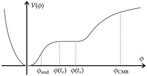
Figure 1: Schematic picture of the inflaton potential realizing PBH formation. When the inflaton is around $\phi_{\mathrm{CMB}}$, scales probed by CMB observations leave the horizon and it is in the SR regime. It enters an extremely flat region at $t=t_{s}$ undergoing an USR period. It enters the SR period again at $t=t_{e}$ until $\phi_{\mathrm{end}}$, the end of inflation.

Small perturbation from the homogeneous part, $\phi(t)$, of the inflaton $\phi(\mathbf{x},t)$ and metric can be expressed as

$$\phi(\mathbf{x},t)=\phi(t)+\delta\phi(\mathbf{x},t),$$

$$\mathrm{d}s^{2}=-N^{2}\mathrm{d}t^{2}+\gamma_{ij}(\mathrm{d}x^{i}+N^{i}\mathrm{d}t)(\mathrm{d}x^{j}+N^{j}\mathrm{d}t),$$ (8)

where $\gamma_{ij}$ is the three-dimensional metric on slices of constant $t$, $N$ is the lapse function, and $N^{i}$ is the shift vector. We choose comoving gauge condition

$$\delta\phi(\mathbf{x},t)=0,~{}\gamma_{ij}(\mathbf{x},t)=a^{2}(t)e^{2\zeta(\mathbf{x},t)}\delta_{ij},$$ (9)

where $\zeta(\mathbf{x},t)$ is curvature perturbation. Here, tensor perturbation is not relevant. Also, $N$ and $N^{i}$ are obtained by solving constraint equations.

Expanding the action (1) up to the second-order of the curvature perturbation yields

$$S^{(2)}[\zeta]=M_{\mathrm{pl}}^{2}\int\mathrm{d}t~{}\mathrm{d}^{3}x~{}a^{3}\epsilon\left[\dot{\zeta}^{2}-\frac{1}{a^{2}}(\partial_{i}\zeta)^{2}\right].$$ (10)

In terms of Mukhanov-Sasaki variable $v=zM_{\mathrm{pl}}\zeta$, where $z=a\sqrt{2\epsilon}$, the action becomes canonically normalized

$$S^{(2)}_{\mathrm{can}}[v]=\frac{1}{2}\int\mathrm{d}\tau~{}\mathrm{d}^{3}x\left[(v^{\prime})^{2}-(\partial_{i}v)^{2}+\frac{z^{\prime\prime}}{z}v^{2}\right],$$ (11)

where a prime denotes derivative with respect to $\tau$. In momentum space, quantization is performed by promoting the Mukhanov-Sasaki variable as an operator

$$v_{\mathbf{k}}(\tau)=M_{\mathrm{pl}}z\zeta_{\mathbf{k}}(\tau)=v_{k}(\tau)\hat{a}_{\mathbf{k}}+v^{*}_{k}(\tau)\hat{a}_{-\mathbf{k}}^{\dagger},$$ (12)

where mode function $v_{k}(\tau)$ approximately satisfies

$$v_{k}^{\prime\prime}+\left(k^{2}-\frac{2}{\tau^{2}}\right)v_{k}=0,$$ (13)

in both SR and USR regimes, and the operators satisfy the commutation relation $[\hat{a}_{\mathbf{k}},\hat{a}_{-\mathbf{k^{\prime}}}^{\dagger}]=(2\pi)^{3}\delta(\mathbf{k}+\mathbf{k^{\prime}})$ under the normalization condition

$$v_{k}^{\prime*}v_{k}-v_{k}^{\prime}v_{k}^{*}=i.$$ (14)

The general solution of mode function $v_{k}(\tau)$ is

$$v_{k}(\tau)=\frac{\mathcal{A}_{k}}{\sqrt{2k}}\left(1-\frac{i}{k\tau}\right)e^{-ik\tau}+\frac{\mathcal{B}_{k}}{\sqrt{2k}}\left(1+\frac{i}{k\tau}\right)e^{ik\tau},$$ (15)

where $\mathcal{A}_{k}$ and $\mathcal{B}_{k}$ are determined by boundary conditions or definition of a vacuum state.

At an early time, $t\lesssim t_{s}$, the inflaton was in SR period with Bunch-Davies initial vacuum. Then the mode function of the curvature perturbation $\zeta_{k}=v_{k}/zM_{\mathrm{pl}}$ is given by

$$\zeta_{k}(\tau)=\left(\frac{iH}{2M_{\mathrm{pl}}\sqrt{\epsilon_{\mathrm{SR}}}}\right)_{\star}\frac{1}{k^{3/2}}\times\left[\mathcal{A}_{1,k}e^{-ik\tau}(1+ik\tau)-\mathcal{B}_{1,k}e^{ik\tau}(1-ik\tau)\right],$$ (16)

with the particular choice of $\mathcal{A}_{1,k}=1$ and $\mathcal{B}_{1,k}=0$. Here $\epsilon_{\mathrm{SR}}$ is $\epsilon$ in SR period and subscript $\star$ denotes the value at the horizon crossing epoch $\tau=-1/k$.

At $t_{s}\lesssim t\lesssim t_{e}$, the inflaton is in USR period. We define $\tau_{s}$ and $\tau_{e}$ as conformal time corresponding to $t_{s}$ and $t_{e}$, respectively. The SR parameter $\epsilon$ can be written as $\epsilon(\tau)=\epsilon_{\mathrm{SR}}(\tau/\tau_{s})^{6}$ based on proportionality in (6). Therefore, the curvature perturbation becomes

$$\zeta_{k}(\tau)=\left(\frac{iH}{2M_{\mathrm{pl}}\sqrt{\epsilon_{\mathrm{SR}}}}\right)_{\star}\left(\frac{\tau_{s}}{\tau}\right)^{3}\frac{1}{k^{3/2}}\times\left[\mathcal{A}_{2,k}e^{-ik\tau}(1+ik\tau)-\mathcal{B}_{2,k}e^{ik\tau}(1-ik\tau)\right],$$ (17)

where coefficients $\mathcal{A}_{2,k}$ and $\mathcal{B}_{2,k}$ are determined by matching to the SR solution (16) at the boundary. We consider instantaneous transition from SR to USR, because it is a good approximation to numerical solutions [32]. Solutions of the coefficients by requiring continuity of $\zeta_{k}(\tau)$ and $\zeta_{k}^{\prime}(\tau)$ at transition $\tau=\tau_{s}$ are

$$\mathcal{A}_{2,k}=1-\frac{3(1+k^{2}\tau_{s}^{2})}{2ik^{3}\tau_{s}^{3}},$$ (18)

$$\mathcal{B}_{2,k}=-\frac{3(1+ik\tau_{s})^{2}}{2ik^{3}\tau_{s}^{3}}e^{-2ik\tau_{s}}.$$ (19)

At late time, $t\gtrsim t_{e}$, the inflaton goes back to SR dynamics. The curvature perturbation can be written as

$$\zeta_{k}(\tau)=\left(\frac{iH}{2M_{\mathrm{pl}}\sqrt{\epsilon_{\mathrm{SR}}}}\right)_{\star}\left(\frac{\tau_{s}}{\tau_{e}}\right)^{3}\frac{1}{k^{3/2}}\times\left[\mathcal{A}_{3,k}e^{-ik\tau}(1+ik\tau)-\mathcal{B}_{3,k}e^{ik\tau}(1-ik\tau)\right],$$ (20)

where coefficients $\mathcal{A}_{3,k}$ and $\mathcal{B}_{3,k}$ are determined by matching to the USR solution (17) at the boundary. Solutions of the coefficients by requiring continuity of $\zeta_{k}(\tau)$ and $\zeta_{k}^{\prime}(\tau)$ at transition $\tau=\tau_{e}$ are

$$\mathcal{A}_{3,k}=\frac{-1}{4k^{6}\tau_{s}^{3}\tau_{e}^{3}}\left\{9(k\tau_{s}-i)^{2}(k\tau_{e}+i)^{2}e^{2ik(\tau_{e}-\tau_{s})}-[k^{2}\tau_{s}^{2}(2k\tau_{s}+3i)+3i][k^{2}\tau_{e}^{2}(2k\tau_{e}-3i)-3i]\right\},$$ (21)

$$\mathcal{B}_{3,k}=\frac{3}{4k^{6}\tau_{s}^{3}\tau_{e}^{3}}\left\{e^{-2ik\tau_{s}}[3+k^{2}\tau_{e}^{2}(3-2ik\tau_{e})](k\tau_{s}-i)^{2}+ie^{-2ik\tau_{e}}[3i+k^{2}\tau_{s}^{2}(2k\tau_{s}+3i)](k\tau_{e}-i)^{2}\right\}.$$ (22)

The two-point functions of curvature perturbation and power spectrum can be written as

$$\left\langle\zeta_{\mathbf{k}}(\tau)\zeta_{\mathbf{k}^{\prime}}(\tau)\right\rangle\equiv(2\pi)^{3}\delta^{3}(\mathbf{k}+\mathbf{k^{\prime}})\left\langle\!\left\langle\zeta_{\mathbf{k}}(\tau)\zeta_{-\mathbf{k}}(\tau)\right\rangle\!\right\rangle,$$ (23)

$$\Delta^{2}_{s}(k,\tau)\equiv\frac{k^{3}}{2\pi^{2}}\left\langle\!\left\langle\zeta_{\mathbf{k}}(\tau)\zeta_{-\mathbf{k}}(\tau)\right\rangle\!\right\rangle,$$ (24)

the bracket $\langle\cdots\rangle=\bra{0}\cdots\ket{0}$ denotes the vacuum expectation value (VEV), and $\Delta^{2}_{s}(k)$ is the power spectrum multiplied by the phase space density. We define $k_{s}$ and $k_{e}$ as wavenumbers which cross the horizon at $\tau_{s}$ and $\tau_{e}$, respectively. At the end of inflation, $\tau_{0}~{}(\rightarrow 0)$, the tree-level power spectrum is

$$\Delta^{2}_{s(0)}(k,\tau_{0})=\frac{k^{3}}{2\pi^{2}}\absolutevalue{\zeta_{k}(\tau_{0})}^{2}=\left(\frac{H^{2}}{8\pi^{2}M_{\mathrm{pl}}^{2}\epsilon_{\mathrm{SR}}}\right)_{\star}\left(\frac{k_{e}}{k_{s}}\right)^{6}\absolutevalue{\mathcal{A}_{3,k}-\mathcal{B}_{3,k}}^{2},$$ (25)

where coefficients $\mathcal{A}_{3,k}$ and $\mathcal{B}_{3,k}$ are given by (21) and (22), respectively.

On large scale, the power spectrum approaches an almost scale-invariant limit

$$\Delta_{s(\mathrm{SR})}^{2}(k)\equiv\Delta^{2}_{s(0)}(k\ll k_{s},\tau_{0})=\left(\frac{H^{2}}{8\pi^{2}M_{\mathrm{pl}}^{2}\epsilon_{\mathrm{SR}}}\right)_{\star},$$ (26)

with a small wavenumber dependence due to the horizon crossing condition manifested in the spectral tilt

$$n_{s}-1=\frac{\mathrm{d}\log\Delta_{s(\mathrm{SR})}^{2}}{\mathrm{d}\log k}=-2\epsilon_{\mathrm{SR}}-\eta_{\mathrm{SR}},$$ (27)

where $\eta_{\mathrm{SR}}$ is $\eta$ in SR period. This large-scale limit must be consistent with CMB observation. On small scale with larger wavenumber, $k_{s}\lesssim k\lesssim k_{e}$, the power spectrum is oscillating around

$$\Delta_{s(\mathrm{PBH})}^{2}\approx\Delta_{s(\mathrm{SR})}^{2}(k_{s})\left(\frac{k_{e}}{k_{s}}\right)^{6},$$ (28)

whose high-density peak may collapse into PBHs. It is amplified by factor $(k_{e}/k_{s})^{6}$ compared to the CMB-scale power spectrum. Plot of the typical power spectrum is shown in Fig. 2.

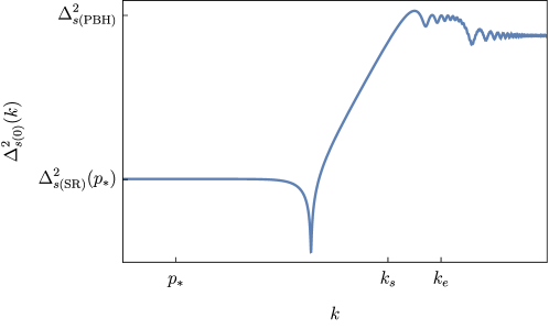
Figure 2: Power spectrum of the curvature perturbation. At CMB scale, $k\ll k_{s}$, the power spectrum is almost scale invariant. $p_{*}=0.05~{}\mathrm{Mpc}^{-1}$ is the pivot scale with amplitude $\Delta_{s(\mathrm{SR})}^{2}(p_{*})=2.1\times 10^{-9}$, based on observational result [11]. At small scale, between $k_{s}$ and $k_{e}$, the power spectrum is amplified to typically $\Delta_{s(\mathrm{PBH})}^{2}\sim\mathcal{O}(0.01)$ to form appreciable amount of PBHs.

III Three-point functions

Three-point functions is generated by cubic self-interaction. Expanding (1) to third-order of $\zeta$ yields the interaction action [36]

$$S^{(3)}[\zeta]=S_{\mathrm{bulk}}[\zeta]+S_{\mathrm{B}}[\zeta]+M_{\mathrm{pl}}^{2}\int\mathrm{d}t~{}\mathrm{d}^{3}x~{}2f(\zeta)\left(\frac{\delta L}{\delta\zeta}\right)_{1},$$ (29)

where the explicit form will be given shortly. The bulk interaction $S_{\mathrm{bulk}}[\zeta]$ reads

$$S_{\mathrm{bulk}}[\zeta]=M_{\mathrm{pl}}^{2}\int\mathrm{d}t~{}\mathrm{d}^{3}x~{}a^{3}\left[\epsilon^{2}\dot{\zeta}^{2}\zeta+\frac{1}{a^{2}}\epsilon^{2}(\partial_{i}\zeta)^{2}\zeta-2\epsilon\dot{\zeta}\partial_{i}\zeta\partial_{i}\chi-\frac{1}{2}\epsilon^{3}\dot{\zeta}^{2}\zeta+\frac{1}{2}\epsilon\zeta(\partial_{i}\partial_{j}\chi)^{2}+\frac{1}{2}\epsilon\dot{\eta}\dot{\zeta}\zeta^{2}\right],$$ (30)

where $\chi=\epsilon\partial^{-2}\dot{\zeta}$. The boundary interaction $S_{\mathrm{B}}[\zeta]$ reads [37]

$$S_{\mathrm{B}}[\zeta]=M_{\mathrm{pl}}^{2}\int\mathrm{d}t~{}\mathrm{d}^{3}x~{}\frac{\mathrm{d}}{\mathrm{d}t} \left[-9a^{3}H\zeta^{3}+\frac{a}{H}\zeta(\partial_{i}\zeta)^{2}-\frac{1}{4aH^{3}}(\partial_{i}\zeta)^{2}\partial^{2}\zeta-\frac{a\epsilon}{H}\zeta(\partial_{i}\zeta)^{2}\right.$$ (31)

$$\left.+\frac{a}{2H^{2}}\zeta(\partial_{i}\partial_{j}\zeta\partial_{i}\partial_{j}\chi-\partial^{2}\zeta\partial^{2}\chi)-\frac{a^{3}}{2H^{2}}\zeta(\partial_{i}\partial_{j}\chi\partial_{i}\partial_{j}\chi-\partial^{2}\chi\partial^{2}\chi)-\frac{\epsilon a^{3}}{H}\zeta\dot{\zeta}^{2}-\frac{\eta a^{3}}{2}\zeta^{2}\partial^{2}\chi\right],$$

where total spatial derivatives are omitted. Boundary interactions without $\dot{\zeta}$ are unimportant because they will not contribute to the correlation of $\zeta$. The last term is interaction proportional to the equation of motion in the lowest order,

$$\left(\frac{\delta L}{\delta\zeta}\right)_{1}=\frac{\mathrm{d}}{\mathrm{d}t}(\epsilon a^{3}\dot{\zeta})-\epsilon a\partial^{2}\zeta.$$ (32)

The function $f(\zeta)$ is explicitly given by

$$f(\zeta)=\frac{\eta}{4}\zeta^{2}+\frac{\dot{\zeta}}{H}\zeta+\frac{1}{4a^{2}H^{2}}[-(\partial_{i}\zeta)^{2}+\partial^{-2}\partial_{i}\partial_{j}(\partial_{i}\zeta\partial_{j}\zeta)]+\frac{1}{2H}[\partial_{i}\zeta\partial_{i}\chi-\partial^{-2}\partial_{i}\partial_{j}(\partial_{i}\zeta\partial_{j}\chi)].$$ (33)

Performing field redefinition $\zeta=\bm{\zeta}+f(\bm{\zeta})$ generates a third-order terms from the second-order action (10) as

$$S^{(2)}[\zeta]=S^{(2)}[\bm{\zeta}]+\int\mathrm{d}t~{}\mathrm{d}^{3}x \left[(-2)f(\bm{\zeta})\left(\frac{\delta L}{\delta\bm{\zeta}}\right)_{1}-\frac{\mathrm{d}}{\mathrm{d}t}\left(\frac{a}{2H^{2}}\bm{\zeta}(\partial_{i}\partial_{j}\bm{\zeta}\partial_{i}\partial_{j}\bm{\chi}-\partial^{2}\bm{\zeta}\partial^{2}\bm{\chi})\right.\right.$$

$$\left.\left.-\frac{a^{3}}{2H^{2}}\bm{\zeta}(\partial_{i}\partial_{j}\bm{\chi}\partial_{i}\partial_{j}\bm{\chi}-\partial^{2}\bm{\chi}\partial^{2}\bm{\chi})-\frac{\epsilon a^{3}}{H}\bm{\zeta}\dot{\bm{\zeta}}^{2}-\frac{\eta a^{3}}{2}\bm{\zeta}^{2}\partial^{2}\bm{\chi}\right)\right],$$ (34)

where $\bm{\chi}=\epsilon\partial^{-2}\dot{\bm{\zeta}}$. Such additional third-order action cancels the last term in (29) and all the boundary interactions including $\dot{\zeta}$ in (31), so the total action is [37]

$$S^{(2)}[\zeta]+S^{(3)}[\zeta]=S^{(2)}[\bm{\zeta}]+S_{\mathrm{bulk}}[\bm{\zeta}].$$ (35)

In terms of $\bm{\zeta}$, the total action is simply given by the second-order action (10) and bulk interaction (30). The interaction Hamiltonian in terms of $\bm{\zeta}$ is

$$H_{\mathrm{int}}(\tau)=-M_{\mathrm{pl}}^{2}\int\mathrm{d}^{3}x~{}a^{2}\left[\epsilon^{2}(\bm{\zeta}^{\prime})^{2}\bm{\zeta}+\epsilon^{2}(\partial_{i}\bm{\zeta})^{2}\bm{\zeta}-2\epsilon^{2}\bm{\zeta}^{\prime}\partial_{i}\bm{\zeta}\partial_{i}\partial^{-2}\bm{\zeta}^{\prime}-\frac{1}{2}\epsilon^{3}(\bm{\zeta}^{\prime})^{2}\bm{\zeta}+\frac{1}{2}\epsilon^{3}\bm{\zeta}(\partial_{i}\partial_{j}\partial^{-2}\bm{\zeta}^{\prime})^{2}+\frac{1}{2}\epsilon\eta^{\prime}\bm{\zeta}^{\prime}\bm{\zeta}^{2}\right].$$ (36)

In the standard SR inflation without PBH formation, the first three terms and last three terms of (36) have coupling $\mathcal{O}(\epsilon^{2})$ and $\mathcal{O}(\epsilon^{3})$, respectively. However, for inflation model with PBH formation, everything is the same except the last term of (36) becomes $\mathcal{O}(\epsilon)$ because $\eta$ has $\mathcal{O}(1)$ transition [39, 40, 41, 42, 43]. Therefore, the leading interaction is

$$H_{\mathrm{int}}(\tau)=-\frac{1}{2}M_{\mathrm{pl}}^{2}\int\mathrm{d}^{3}x~{}a^{2}\epsilon\eta^{\prime}\bm{\zeta}^{\prime}\bm{\zeta}^{2}.$$ (37)

Three-point functions of $\zeta$ can be written schematically as

$$\langle\zeta_{\mathbf{k}_{1}}(\tau)\zeta_{\mathbf{k}_{2}}(\tau)\zeta_{\mathbf{k}_{3}}(\tau)\rangle=\langle\bm{\zeta}_{\mathbf{k}_{1}}(\tau)\bm{\zeta}_{\mathbf{k}_{2}}(\tau)\bm{\zeta}_{\mathbf{k}_{3}}(\tau)\rangle+\mathrm{redefinition~{}terms},$$ (38)

where the first term is generated by bulk interaction (36) and the second term is boundary contribution at $\tau$ from field redefinition. Higher-order correction to the expectation value of an operator $\mathcal{O}(\tau)$ is calculated by the in-in perturbation theory

$$\langle\mathcal{O(\tau)}\rangle=\left\langle\left[\bar{\mathrm{T}}\exp\left(i\int_{-\infty}^{\tau}\mathrm{d}\tau^{\prime}H_{\mathrm{int}}(\tau^{\prime})\right)\right]\mathcal{\hat{O}}(\tau)\left[\mathrm{T}\exp\left(-i\int_{-\infty}^{\tau}\mathrm{d\tau^{\prime}}H_{\mathrm{int}}(\tau^{\prime})\right)\right]\right\rangle,$$ (39)

where $\mathrm{T}$ and $\bar{\mathrm{T}}$ denote time and antitime ordering. For three-point functions, the operator is $\bm{\zeta}_{\mathbf{k}_{1}}(\tau)\bm{\zeta}_{\mathbf{k}_{2}}(\tau)\bm{\zeta}_{\mathbf{k}_{3}}(\tau)$. First-order expansion of (39) reads

$$\langle\mathcal{O(\tau)}\rangle=2\int_{-\infty}^{\tau}\mathrm{d}\tau_{1}~{}\mathrm{Im}\left\langle\mathcal{\hat{O}}(\tau)H_{\mathrm{int}}(\tau_{1})\right\rangle.$$ (40)

Bispectrum $\left\langle\!\left\langle\zeta_{\mathbf{k}_{1}}(\tau)\zeta_{\mathbf{k}_{2}}(\tau)\zeta_{\mathbf{k}_{3}}(\tau)\right\rangle\!\right\rangle$ is defined as

$$\langle\zeta_{\mathbf{k}_{1}}(\tau)\zeta_{\mathbf{k}_{2}}(\tau)\zeta_{\mathbf{k}_{3}}(\tau)\rangle=(2\pi)^{3}\delta(\mathbf{k}_{1}+\mathbf{k}_{2}+\mathbf{k}_{3})\left\langle\!\left\langle\zeta_{\mathbf{k}_{1}}(\tau)\zeta_{\mathbf{k}_{2}}(\tau)\zeta_{\mathbf{k}_{3}}(\tau)\right\rangle\!\right\rangle.$$ (41)

The squeezed limit, when one of wavenumbers in the bispectrum is very small, the bispectrum satisfies Maldacena’s theorem [36]

$$\lim_{k_{1}\rightarrow 0}\left\langle\!\left\langle\zeta_{\mathbf{k}_{1}}(\tau)\zeta_{\mathbf{k}_{2}}(\tau)\zeta_{-\mathbf{k}_{2}}(\tau)\right\rangle\!\right\rangle =-(n_{s}(k_{2},\tau)-1)\left\langle\!\left\langle\zeta_{\mathbf{k}_{2}}(\tau)\zeta_{-\mathbf{k}_{2}}(\tau)\right\rangle\!\right\rangle\left\langle\!\left\langle\zeta_{\mathbf{k}_{1}}(\tau)\zeta_{-\mathbf{k}_{1}}(\tau)\right\rangle\!\right\rangle$$

$$=-(n_{s}(k_{2},\tau)-1)\absolutevalue{\zeta_{k_{2}}(\tau)}^{2}\absolutevalue{\zeta_{k_{1}}(\tau)}^{2},$$ (43)

where we define

$$n_{s}(k,\tau)-1=\frac{\mathrm{d}\log\Delta_{s}^{2}(k,\tau)}{\mathrm{d}\log k}.$$ (44)

We emphasize that Maldacena’s theorem is satisfied by the bispectrum of $\zeta$, not $\bm{\zeta}$. We now calculate the bispectrum at four different epochs.

III.1 Slightly after the end of USR period

In this subsection, we calculate bispectrum at a time slightly after the end of the USR period. Note that every time $\tau_{e}$ is written in this subsection implicitly means it is evaluated at $\tau_{e}^{+}$ when the inflaton is already in the second SR period. The three-point functions of $\bm{\zeta}$ is given by

$$\langle\bm{\zeta}_{\mathbf{k}_{1}}(\tau_{e})\bm{\zeta}_{\mathbf{k}_{2}}(\tau_{e})\bm{\zeta}_{\mathbf{k}_{3}}(\tau_{e})\rangle=2\int_{-\infty}^{\tau_{e}}\mathrm{d}\tau_{1}~{}\mathrm{Im}\left\langle\bm{\zeta}_{\mathbf{k}_{1}}(\tau)\bm{\zeta}_{\mathbf{k}_{2}}(\tau)\bm{\zeta}_{\mathbf{k}_{3}}(\tau)H_{\mathrm{int}}(\tau_{1})\right\rangle.$$ (45)

Substituting (37) yields bispectrum

$$\left\langle\!\left\langle\bm{\zeta}_{\mathbf{k}_{1}}(\tau_{e})\bm{\zeta}_{\mathbf{k}_{2}}(\tau_{e})\bm{\zeta}_{\mathbf{k}_{3}}(\tau_{e})\right\rangle\!\right\rangle=-2M_{\mathrm{pl}}^{2}\int_{-\infty}^{\tau_{e}}\mathrm{d}\tau_{1}\epsilon(\tau_{1})\eta^{\prime}(\tau_{1})a^{2}(\tau_{1})\mathrm{Im}\left[\zeta_{k_{1}}(\tau_{e})\zeta_{k_{2}}(\tau_{e})\zeta_{k_{3}}(\tau_{e})\zeta_{\tilde{k}_{1}}^{*}(\tau_{1})\zeta_{\tilde{k}_{2}}^{*}(\tau_{1})\zeta_{\tilde{k}_{3}}^{\prime*}(\tau_{1})\right]+\mathrm{perm}.$$ (46)

Here and hereafter, $+\mathrm{perm}$ means summation over a cyclic permutation of suffices with a tilde in the preceeding expression. To evaluate the time integral, we remind that $\eta$ is almost constant in both SR and USR periods, so $\eta^{\prime}(\tau)\approx 0$ except for sharp transitions around $\tau=\tau_{s}$ and $\tau=\tau_{e}$. Therefore, $\eta^{\prime}(\tau)$ can be written as

$$\eta^{\prime}(\tau)=\Delta\eta[-\delta(\tau-\tau_{s})+\delta(\tau-\tau_{e})],$$ (47)

where $\Delta\eta\approx 6$. After evaluating the time integral, the bispectrum becomes

$$\left\langle\!\left\langle\bm{\zeta}_{\mathbf{k}_{1}}(\tau_{e})\bm{\zeta}_{\mathbf{k}_{2}}(\tau_{e})\bm{\zeta}_{\mathbf{k}_{3}}(\tau_{e})\right\rangle\!\right\rangle= -2M_{\mathrm{pl}}^{2}\epsilon(\tau_{e})a^{2}(\tau_{e})\Delta\eta~{}\zeta_{k_{1}}(\tau_{e})\zeta_{\tilde{k}_{1}}^{*}(\tau_{e})\zeta_{k_{2}}(\tau_{e})\zeta_{\tilde{k}_{2}}^{*}(\tau_{e})\mathrm{Im}(\zeta_{k_{3}}(\tau_{e})\zeta_{\tilde{k}_{3}}^{\prime*}(\tau_{e}))$$

$$+2M_{\mathrm{pl}}^{2}\epsilon(\tau_{s})a^{2}(\tau_{s})\Delta\eta~{}\mathrm{Im}\left[\zeta_{k_{1}}(\tau_{e})\zeta_{k_{2}}(\tau_{e})\zeta_{k_{3}}(\tau_{e})\zeta_{\tilde{k}_{1}}^{*}(\tau_{s})\zeta_{\tilde{k}_{2}}^{*}(\tau_{s})\zeta_{\tilde{k}_{3}}^{\prime*}(\tau_{s})\right]+\mathrm{perm}.$$ (48)

From normalization condition (14), we can obtain

$$\mathrm{Im}(\zeta_{k}(\tau_{e})\zeta_{k}^{\prime*}(\tau_{e}))=\frac{1}{4M_{\mathrm{pl}}^{2}\epsilon(\tau_{e})a^{2}(\tau_{e})}.$$ (49)

Substituting it to (48), we find the squeezed limit of bispectrum as

$$\left\langle\!\left\langle\bm{\zeta}_{\mathbf{k}_{1}}(\tau_{e})\bm{\zeta}_{\mathbf{k}_{2}}(\tau_{e})\bm{\zeta}_{-\mathbf{k}_{2}}(\tau_{e})\right\rangle\!\right\rangle=-\left\{\Delta\eta-4\Delta\eta M_{\mathrm{pl}}^{2}\epsilon(\tau_{s})a^{2}(\tau_{s})\mathrm{Im}\left[\frac{\zeta_{k_{2}}^{2}(\tau_{e})}{\absolutevalue{\zeta_{k_{2}}(\tau_{e})}^{2}}\zeta_{k_{2}}^{*}(\tau_{s})\zeta_{k_{2}}^{\prime*}(\tau_{s})\right]\right\}\absolutevalue{\zeta_{k_{1}}(\tau_{e})}^{2}\absolutevalue{\zeta_{k_{2}}(\tau_{e})}^{2}.$$ (50)

We define the coefficient $C(k)=C_{e}(k)+C_{s}(k)$, where

$$C_{e}(k)=\Delta\eta,~{}C_{s}(k)=-4\Delta\eta M_{\mathrm{pl}}^{2}\epsilon(\tau_{s})a^{2}(\tau_{s})\mathrm{Im}\left[\frac{\zeta_{k}^{2}(\tau_{e})}{\absolutevalue{\zeta_{k}(\tau_{e})}^{2}}\zeta_{k}^{*}(\tau_{s})\zeta_{k}^{\prime*}(\tau_{s})\right].$$ (51)

Plot of $C_{e}(k)$ and $C_{s}(k)$ are shown in Fig. 3. For comparison, we also plot $n_{s}(k,\tau_{e})-1$ directly from the mode function (17). We can see that $C_{s}(k)$ almost overlaps with $n_{s}(k,\tau_{e})-1$, but they are not precisely equal. Clearly, the coefficient $C(k)\neq n_{s}(k,\tau_{e})-1$, implies that the bispectrum of $\bm{\zeta}$ does not satisfy Maldacena’s theorem.

The bispectrum of $\zeta$ is given by the bispectrum of $\bm{\zeta}$ plus contribution from field redefinition. Because $\eta(\tau_{e})\approx 0$, the leading field redefinition (33) is $\dot{\bm{\zeta}}\bm{\zeta}/H$. Noting that $a(\tau_{e})H=k_{e}$, the bispectrum of $\zeta$ reads

$$\left\langle\!\left\langle\zeta_{\mathbf{k}_{1}}(\tau_{e})\zeta_{\mathbf{k}_{2}}(\tau_{e})\zeta_{\mathbf{k}_{3}}(\tau_{e})\right\rangle\!\right\rangle= \left\langle\!\left\langle\bm{\zeta}_{\mathbf{k}_{1}}(\tau_{e})\bm{\zeta}_{\mathbf{k}_{2}}(\tau_{e})\bm{\zeta}_{\mathbf{k}_{3}}(\tau_{e})\right\rangle\!\right\rangle+$$

$$k_{e}^{-1}\left[\langle\!\langle\bm{\zeta}_{\mathbf{k}_{2}}^{\prime}(\tau_{e})\bm{\zeta}_{-\mathbf{k}_{2}}(\tau_{e})\rangle\!\rangle\left\langle\!\left\langle\bm{\zeta}_{\mathbf{k}_{3}}(\tau_{e})\bm{\zeta}_{-\mathbf{k}_{3}}(\tau_{e})\right\rangle\!\right\rangle+\left\langle\!\left\langle\bm{\zeta}_{\mathbf{k}_{2}}(\tau_{e})\bm{\zeta}_{-\mathbf{k}_{2}}(\tau_{e})\right\rangle\!\right\rangle\langle\!\langle\bm{\zeta}_{\mathbf{k}_{3}}^{\prime}(\tau_{e})\bm{\zeta}_{-\mathbf{k}_{3}}(\tau_{e})\rangle\!\rangle\right.$$

$$\left.+\left\langle\!\left\langle\bm{\zeta}_{\mathbf{k}_{1}}(\tau_{e})\bm{\zeta}_{-\mathbf{k}_{1}}(\tau_{e})\right\rangle\!\right\rangle\langle\!\langle\bm{\zeta}_{\mathbf{k}_{3}}^{\prime}(\tau_{e})\bm{\zeta}_{-\mathbf{k}_{3}}(\tau_{e})\rangle\!\rangle+\langle\!\langle\bm{\zeta}_{\mathbf{k}_{1}}(\tau_{e})\bm{\zeta}_{-\mathbf{k}_{1}}^{\prime}(\tau_{e})\rangle\!\rangle\left\langle\!\left\langle\bm{\zeta}_{\mathbf{k}_{3}}(\tau_{e})\bm{\zeta}_{-\mathbf{k}_{3}}(\tau_{e})\right\rangle\!\right\rangle\right.$$

$$\left.+\left\langle\!\left\langle\bm{\zeta}_{\mathbf{k}_{1}}(\tau_{e})\bm{\zeta}_{-\mathbf{k}_{1}}(\tau_{e})\right\rangle\!\right\rangle\langle\!\langle\bm{\zeta}_{\mathbf{k}_{2}}(\tau_{e})\bm{\zeta}_{-\mathbf{k}_{2}}^{\prime}(\tau_{e})\rangle\!\rangle+\langle\!\langle\bm{\zeta}_{\mathbf{k}_{1}}(\tau_{e})\bm{\zeta}_{-\mathbf{k}_{1}}^{\prime}(\tau_{e})\rangle\!\rangle\left\langle\!\left\langle\bm{\zeta}_{\mathbf{k}_{2}}(\tau_{e})\bm{\zeta}_{-\mathbf{k}_{2}}(\tau_{e})\right\rangle\!\right\rangle\right].$$ (52)

The leading terms in squeezed limit, $k_{1}\rightarrow 0$, are

$$\left\langle\!\left\langle\zeta_{\mathbf{k}_{1}}(\tau_{e})\zeta_{\mathbf{k}_{2}}(\tau_{e})\zeta_{-\mathbf{k}_{2}}(\tau_{e})\right\rangle\!\right\rangle= \left\langle\!\left\langle\bm{\zeta}_{\mathbf{k}_{1}}(\tau_{e})\bm{\zeta}_{\mathbf{k}_{2}}(\tau_{e})\bm{\zeta}_{-\mathbf{k}_{2}}(\tau_{e})\right\rangle\!\right\rangle$$

$$+k_{e}^{-1}\left\langle\!\left\langle\bm{\zeta}_{\mathbf{k}_{1}}(\tau_{e})\bm{\zeta}_{-\mathbf{k}_{1}}(\tau_{e})\right\rangle\!\right\rangle\left[\langle\!\langle\bm{\zeta}_{\mathbf{k}_{2}}^{\prime}(\tau_{e})\bm{\zeta}_{-\mathbf{k}_{2}}(\tau_{e})\rangle\!\rangle+\langle\!\langle\bm{\zeta}_{\mathbf{k}_{2}}(\tau_{e})\bm{\zeta}_{-\mathbf{k}_{2}}^{\prime}(\tau_{e})\rangle\!\rangle\right],$$ (53)

and more explicitly

$$\left\langle\!\left\langle\zeta_{\mathbf{k}_{1}}(\tau_{e})\zeta_{\mathbf{k}_{2}}(\tau_{e})\zeta_{-\mathbf{k}_{2}}(\tau_{e})\right\rangle\!\right\rangle=- \left\{\Delta\eta-4\Delta\eta M_{\mathrm{pl}}^{2}\epsilon(\tau_{s})a^{2}(\tau_{s})\mathrm{Im}\left[\frac{\zeta_{k_{2}}^{2}(\tau_{e})}{\absolutevalue{\zeta_{k_{2}}(\tau_{e})}^{2}}\zeta_{k_{2}}^{*}(\tau_{s})\zeta_{k_{2}}^{\prime*}(\tau_{s})\right]\right.$$

$$\left.-2\mathrm{Re}\left[\frac{\zeta_{k_{2}}(\tau_{e})\zeta_{k_{2}}^{\prime*}(\tau_{e})}{k_{e}\absolutevalue{\zeta_{k_{2}}(\tau_{e})}^{2}}\right]\right\}\absolutevalue{\zeta_{k_{1}}(\tau_{e})}^{2}\absolutevalue{\zeta_{k_{2}}(\tau_{e})}^{2}.$$ (54)

We define contribution from field redefinition as

$$B(k)=2\mathrm{Re}\left[\frac{\zeta_{k}(\tau_{e})\zeta_{k}^{\prime*}(\tau_{e})}{k_{e}\absolutevalue{\zeta_{k}(\tau_{e})}^{2}}\right],$$ (55)

so the total coefficient is $T(k)=C(k)-B(k)$. The plot of $B(k)$ and $T(k)$ are shown in Fig. (3). We can see that $T(k)$ precisely equals to $n_{s}(k,\tau_{e})-1$, which confirms Maldacena’s theorem. Equality $T(k)=n_{s}(k,\tau_{e})-1$ holds exactly, which one can confirm by substituting mode function (17) to the explicit form of $T(k)$.

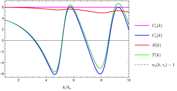
Figure 3: Plot of $C_{e}(k)$, $C_{s}(k)$, $B(k)$, $T(k)$, and $n_{s}(k,\tau_{e})-1$. We choose $k_{e}/k_{s}=10$ just for illustrative purposes.

III.2 Slightly before the end of USR period

In this subsection, we calculate bispectrum at a time slightly before the end of the USR period. Note that every time $\tau_{e}$ is written in this subsection implicitly means it is evaluated at $\tau_{e}^{-}$ when the inflaton is still in the USR period. At this time, there is still no sharp transition at $\tau_{e}$, so the bispectrum of $\bm{\zeta}$ is

$$\left\langle\!\left\langle\bm{\zeta}_{\mathbf{k}_{1}}(\tau_{e})\bm{\zeta}_{\mathbf{k}_{2}}(\tau_{e})\bm{\zeta}_{\mathbf{k}_{3}}(\tau_{e})\right\rangle\!\right\rangle=2M_{\mathrm{pl}}^{2}\epsilon(\tau_{s})a^{2}(\tau_{s})\Delta\eta~{}\mathrm{Im}\left[\zeta_{k_{1}}(\tau_{e})\zeta_{k_{2}}(\tau_{e})\zeta_{k_{3}}(\tau_{e})\zeta_{\tilde{k}_{1}}^{*}(\tau_{s})\zeta_{\tilde{k}_{2}}^{*}(\tau_{s})\zeta_{\tilde{k}_{3}}^{\prime*}(\tau_{s})\right]+\mathrm{perm}.$$ (56)

Because $\eta(\tau_{e})\approx-6$, the leading field redefinition (33) are $\eta\bm{\zeta}^{2}/4$ and $\dot{\bm{\zeta}}\bm{\zeta}/H$. In squeezed limit, the bispectrum of $\zeta$ is

$$\left\langle\!\left\langle\zeta_{\mathbf{k}_{1}}(\tau_{e})\zeta_{\mathbf{k}_{2}}(\tau_{e})\zeta_{-\mathbf{k}_{2}}(\tau_{e})\right\rangle\!\right\rangle= \left\langle\!\left\langle\bm{\zeta}_{\mathbf{k}_{1}}(\tau_{e})\bm{\zeta}_{\mathbf{k}_{2}}(\tau_{e})\bm{\zeta}_{-\mathbf{k}_{2}}(\tau_{e})\right\rangle\!\right\rangle+\frac{\eta(\tau_{e})}{4}4\left\langle\!\left\langle\bm{\zeta}_{\mathbf{k}_{1}}(\tau_{e})\bm{\zeta}_{-\mathbf{k}_{1}}(\tau_{e})\right\rangle\!\right\rangle\left\langle\!\left\langle\bm{\zeta}_{\mathbf{k}_{2}}(\tau_{e})\bm{\zeta}_{-\mathbf{k}_{2}}(\tau_{e})\right\rangle\!\right\rangle$$

$$+k_{e}^{-1}\left\langle\!\left\langle\bm{\zeta}_{\mathbf{k}_{1}}(\tau_{e})\bm{\zeta}_{-\mathbf{k}_{1}}(\tau_{e})\right\rangle\!\right\rangle\left(\langle\!\langle\bm{\zeta}_{\mathbf{k}_{2}}^{\prime}(\tau_{e})\bm{\zeta}_{-\mathbf{k}_{2}}(\tau_{e})\rangle\!\rangle+\langle\!\langle\bm{\zeta}_{\mathbf{k}_{2}}(\tau_{e})\bm{\zeta}_{-\mathbf{k}_{2}}^{\prime}(\tau_{e})\rangle\!\rangle\right).$$ (57)

More explicitly, it can be written as

$$\left\langle\!\left\langle\zeta_{\mathbf{k}_{1}}(\tau_{e})\zeta_{\mathbf{k}_{2}}(\tau_{e})\zeta_{-\mathbf{k}_{2}}(\tau_{e})\right\rangle\!\right\rangle=- \left\{-4\Delta\eta M_{\mathrm{pl}}^{2}\epsilon(\tau_{s})a^{2}(\tau_{s})\mathrm{Im}\left[\frac{\zeta_{k_{2}}^{2}(\tau_{e})}{\absolutevalue{\zeta_{k_{2}}(\tau_{e})}^{2}}\zeta_{k_{2}}^{*}(\tau_{s})\zeta_{k_{2}}^{\prime*}(\tau_{s})\right]\right.$$

$$\left.-2\mathrm{Re}\left[\frac{\zeta_{k_{2}}(\tau_{e})\zeta_{k_{2}}^{\prime*}(\tau_{e})}{k_{e}\absolutevalue{\zeta_{k_{2}}(\tau_{e})}^{2}}\right]+\Delta\eta\right\}\absolutevalue{\zeta_{k_{1}}(\tau_{e})}^{2}\absolutevalue{\zeta_{k_{2}}(\tau_{e})}^{2}.$$ (58)

III.3 Exactly at the end of USR period

In this subsection, we calculate the bispectrum at exactly the end of the USR period. The bispectrum of $\bm{\zeta}$ is

$$\left\langle\!\left\langle\bm{\zeta}_{\mathbf{k}_{1}}(\tau_{e})\bm{\zeta}_{\mathbf{k}_{2}}(\tau_{e})\bm{\zeta}_{\mathbf{k}_{3}}(\tau_{e})\right\rangle\!\right\rangle= -2M_{\mathrm{pl}}^{2}\epsilon(\tau_{e})a^{2}(\tau_{e})\frac{1}{2}\Delta\eta~{}\zeta_{k_{1}}(\tau_{e})\zeta_{\tilde{k}_{1}}^{*}(\tau_{e})\zeta_{k_{2}}(\tau_{e})\zeta_{\tilde{k}_{2}}^{*}(\tau_{e})\mathrm{Im}(\zeta_{k_{3}}(\tau_{e})\zeta_{\tilde{k}_{3}}^{\prime*}(\tau_{e}))$$

$$+2M_{\mathrm{pl}}^{2}\epsilon(\tau_{s})a^{2}(\tau_{s})\Delta\eta~{}\mathrm{Im}\left[\zeta_{k_{1}}(\tau_{e})\zeta_{k_{2}}(\tau_{e})\zeta_{k_{3}}(\tau_{e})\zeta_{\tilde{k}_{1}}^{*}(\tau_{s})\zeta_{\tilde{k}_{2}}^{*}(\tau_{s})\zeta_{\tilde{k}_{3}}^{\prime*}(\tau_{s})\right]+\mathrm{perm},$$ (59)

where factor $1/2$ arises because only the left half of the Dirac-Delta function is integrated. In the squeezed limit, it becomes

$$\left\langle\!\left\langle\bm{\zeta}_{\mathbf{k}_{1}}(\tau_{e})\bm{\zeta}_{\mathbf{k}_{2}}(\tau_{e})\bm{\zeta}_{-\mathbf{k}_{2}}(\tau_{e})\right\rangle\!\right\rangle=-\left\{\frac{1}{2}\Delta\eta-4\Delta\eta M_{\mathrm{pl}}^{2}\epsilon(\tau_{s})a^{2}(\tau_{s})\mathrm{Im}\left[\frac{\zeta_{k_{2}}^{2}(\tau_{e})}{\absolutevalue{\zeta_{k_{2}}(\tau_{e})}^{2}}\zeta_{k_{2}}^{*}(\tau_{s})\zeta_{k_{2}}^{\prime*}(\tau_{s})\right]\right\}\absolutevalue{\zeta_{k_{1}}(\tau_{e})}^{2}\absolutevalue{\zeta_{k_{2}}(\tau_{e})}^{2}.$$ (60)

After adding contribution from field redefinition, the bispectrum of $\zeta$ in squeezed limit is

$$\left\langle\!\left\langle\zeta_{\mathbf{k}_{1}}(\tau_{e})\zeta_{\mathbf{k}_{2}}(\tau_{e})\zeta_{-\mathbf{k}_{2}}(\tau_{e})\right\rangle\!\right\rangle= \left\langle\!\left\langle\bm{\zeta}_{\mathbf{k}_{1}}(\tau_{e})\bm{\zeta}_{\mathbf{k}_{2}}(\tau_{e})\bm{\zeta}_{-\mathbf{k}_{2}}(\tau_{e})\right\rangle\!\right\rangle+\frac{\eta(\tau_{e})}{4}4\left\langle\!\left\langle\bm{\zeta}_{\mathbf{k}_{1}}(\tau_{e})\bm{\zeta}_{-\mathbf{k}_{1}}(\tau_{e})\right\rangle\!\right\rangle\left\langle\!\left\langle\bm{\zeta}_{\mathbf{k}_{2}}(\tau_{e})\bm{\zeta}_{-\mathbf{k}_{2}}(\tau_{e})\right\rangle\!\right\rangle$$

$$+k_{e}^{-1}\left\langle\!\left\langle\bm{\zeta}_{\mathbf{k}_{1}}(\tau_{e})\bm{\zeta}_{-\mathbf{k}_{1}}(\tau_{e})\right\rangle\!\right\rangle\left(\langle\!\langle\bm{\zeta}_{\mathbf{k}_{2}}^{\prime}(\tau_{e})\bm{\zeta}_{-\mathbf{k}_{2}}(\tau_{e})\rangle\!\rangle+\langle\!\langle\bm{\zeta}_{\mathbf{k}_{2}}(\tau_{e})\bm{\zeta}_{-\mathbf{k}_{2}}^{\prime}(\tau_{e})\rangle\!\rangle\right),$$ (61)

and more explicitly

$$\left\langle\!\left\langle\zeta_{\mathbf{k}_{1}}(\tau_{e})\zeta_{\mathbf{k}_{2}}(\tau_{e})\zeta_{-\mathbf{k}_{2}}(\tau_{e})\right\rangle\!\right\rangle=- \left\{\frac{1}{2}\Delta\eta-4\Delta\eta M_{\mathrm{pl}}^{2}\epsilon(\tau_{s})a^{2}(\tau_{s})\mathrm{Im}\left[\frac{\zeta_{k_{2}}^{2}(\tau_{e})}{\absolutevalue{\zeta_{k_{2}}(\tau_{e})}^{2}}\zeta_{k_{2}}^{*}(\tau_{s})\zeta_{k_{2}}^{\prime*}(\tau_{s})\right]\right.$$

$$\left.-2\mathrm{Re}\left[\frac{\zeta_{k_{2}}(\tau_{e})\zeta_{k_{2}}^{\prime*}(\tau_{e})}{k_{e}\absolutevalue{\zeta_{k_{2}}(\tau_{e})}^{2}}\right]-\eta(\tau_{e})\right\}\absolutevalue{\zeta_{k_{1}}(\tau_{e})}^{2}\absolutevalue{\zeta_{k_{2}}(\tau_{e})}^{2}.$$ (62)

We need to define $\eta(\tau_{e})=-\Delta\eta/2$ so the squeezed limit of bispectrum becomes a continuous function from $\tau_{e}^{-}$ to $\tau_{e}^{+}$. Therefore, bispectrum (54), (58), and (62) are equal.

III.4 At the end of inflation

At the end of inflation, $\tau_{0}~{}(\rightarrow 0)$, contribution from field redefinition are negligible because $\eta(\tau_{0})\approx 0$ and $\dot{\zeta}$ decays. Therefore, bispectrum of $\zeta$ and $\bm{\zeta}$ are equal

$$\langle\zeta_{\mathbf{k}_{1}}(\tau_{0})\zeta_{\mathbf{k}_{2}}(\tau_{0})\zeta_{\mathbf{k}_{3}}(\tau_{0})\rangle=\langle\bm{\zeta}_{\mathbf{k}_{1}}(\tau_{0})\bm{\zeta}_{\mathbf{k}_{2}}(\tau_{0})\bm{\zeta}_{\mathbf{k}_{3}}(\tau_{0})\rangle,$$ (63)

and it is given by

$$\left\langle\!\left\langle\zeta_{\mathbf{k}_{1}}(\tau_{0})\zeta_{\mathbf{k}_{2}}(\tau_{0})\zeta_{\mathbf{k}_{3}}(\tau_{0})\right\rangle\!\right\rangle=-2M_{\mathrm{pl}}^{2}\int_{-\infty}^{\tau_{0}}\mathrm{d}\tau_{1}\epsilon(\tau_{1})\eta^{\prime}(\tau_{1})a^{2}(\tau_{1})\mathrm{Im}\left[\zeta_{k_{1}}(\tau_{0})\zeta_{k_{2}}(\tau_{0})\zeta_{k_{3}}(\tau_{0})\zeta_{\tilde{k}_{1}}^{*}(\tau_{1})\zeta_{\tilde{k}_{2}}^{*}(\tau_{1})\zeta_{\tilde{k}_{3}}^{\prime*}(\tau_{1})\right]+\mathrm{perm}.$$ (64)

Substituting (47) to the time integral yields

$$\left\langle\!\left\langle\zeta_{\mathbf{k}_{1}}(\tau_{0})\zeta_{\mathbf{k}_{2}}(\tau_{0})\zeta_{\mathbf{k}_{3}}(\tau_{0})\right\rangle\!\right\rangle= -2M_{\mathrm{pl}}^{2}\epsilon(\tau_{e})a^{2}(\tau_{e})\Delta\eta~{}\mathrm{Im}\left[\zeta_{k_{1}}(\tau_{0})\zeta_{k_{2}}(\tau_{0})\zeta_{k_{3}}(\tau_{0})\zeta_{\tilde{k}_{1}}^{*}(\tau_{e})\zeta_{\tilde{k}_{2}}^{*}(\tau_{e})\zeta_{\tilde{k}_{3}}^{\prime*}(\tau_{e})\right]$$

$$+2M_{\mathrm{pl}}^{2}\epsilon(\tau_{s})a^{2}(\tau_{s})\Delta\eta~{}\mathrm{Im}\left[\zeta_{k_{1}}(\tau_{0})\zeta_{k_{2}}(\tau_{0})\zeta_{k_{3}}(\tau_{0})\zeta_{\tilde{k}_{1}}^{*}(\tau_{s})\zeta_{\tilde{k}_{2}}^{*}(\tau_{s})\zeta_{\tilde{k}_{3}}^{\prime*}(\tau_{s})\right]+\mathrm{perm}.$$ (65)

In the squeezed limit, the bispectrum becomes

$$\left\langle\!\left\langle\zeta_{\mathbf{k}_{1}}(\tau_{0})\zeta_{\mathbf{k}_{2}}(\tau_{0})\zeta_{\mathbf{k}_{3}}(\tau_{0})\right\rangle\!\right\rangle=- \left\{4\Delta\eta M_{\mathrm{pl}}^{2}\epsilon(\tau_{e})a^{2}(\tau_{e})\mathrm{Im}\left[\frac{\zeta_{k_{2}}^{2}(\tau_{0})}{\absolutevalue{\zeta_{k_{2}}(\tau_{0})}^{2}}\zeta_{k_{2}}^{*}(\tau_{e})\zeta_{k_{2}}^{\prime*}(\tau_{e})\right]\right.$$

$$\left.-4\Delta\eta M_{\mathrm{pl}}^{2}\epsilon(\tau_{s})a^{2}(\tau_{s})\mathrm{Im}\left[\frac{\zeta_{k_{2}}^{2}(\tau_{0})}{\absolutevalue{\zeta_{k_{2}}(\tau_{0})}^{2}}\zeta_{k_{2}}^{*}(\tau_{s})\zeta_{k_{2}}^{\prime*}(\tau_{s})\right]\right\}\absolutevalue{\zeta_{k_{1}}(\tau_{0})}^{2}\absolutevalue{\zeta_{k_{2}}(\tau_{0})}^{2}.$$ (66)

We define the coefficient as

$$C_{0}(k)=4\Delta\eta M_{\mathrm{pl}}^{2}\mathrm{Im}\left\{\frac{\zeta_{k}^{2}(\tau_{0})}{\absolutevalue{\zeta_{k}(\tau_{0})}^{2}}\left[\epsilon(\tau_{e})a^{2}(\tau_{e})\zeta_{k}^{*}(\tau_{e})\zeta_{k}^{\prime*}(\tau_{e})-\epsilon(\tau_{s})a^{2}(\tau_{s})\zeta_{k}^{*}(\tau_{s})\zeta_{k}^{\prime*}(\tau_{s})\right]\right\}.$$ (67)

Plot of $C_{0}(k)$ is shown in Fig. 4. For comparison, we also plot $n_{s}(k,\tau_{0})-1$ directly from power spectrum (25). We can see that $C_{0}(k)$ precisely equals to $n_{s}(k,\tau_{0})-1$, which confirms Maldacena’s theorem. The equality $C_{0}(k)=n_{s}(k,\tau_{0})-1$ holds exactly, which one can confirm by substituting mode function (20) to the explicit form of $C_{0}(k)$.

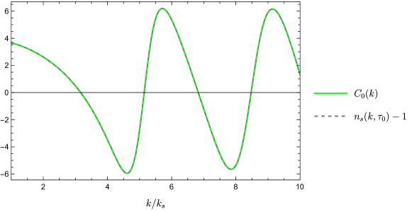
Figure 4: Plot of $C_{0}(k)$ and $n_{s}(k,\tau_{0})-1$. We choose $k_{e}/k_{s}=10$ just for illustrative purposes.

IV One-loop correction

Schematically, one-loop correction to the power spectrum of $\zeta$ can be written as

$$\left\langle\!\left\langle\zeta_{\mathbf{p}}(\tau_{0})\zeta_{-\mathbf{p}}(\tau_{0})\right\rangle\!\right\rangle_{(1)}=\left\langle\!\left\langle\bm{\zeta}_{\mathbf{p}}(\tau_{0})\bm{\zeta}_{-\mathbf{p}}(\tau_{0})\right\rangle\!\right\rangle_{(1)}+\mathrm{redefinition~{}terms}.$$ (68)

The redefinition terms are negligible because they are evaluated at the end of SR period. Thus, one-loop correction at the end of inflation is simply

$$\left\langle\!\left\langle\zeta_{\mathbf{p}}(\tau_{0})\zeta_{-\mathbf{p}}(\tau_{0})\right\rangle\!\right\rangle_{(1)}=\left\langle\!\left\langle\bm{\zeta}_{\mathbf{p}}(\tau_{0})\bm{\zeta}_{-\mathbf{p}}(\tau_{0})\right\rangle\!\right\rangle_{(1)}.$$ (69)

In this section, we calculate the one-loop correction to the large-scale power spectrum by two different methods: source method and direct in-in formalism. The source method utilizes bispectrum to calculate one-loop correction, which is used by [2]. Prior to this work, source method is implemented by [46, 47], in a similar context. On the other hand, direct in-in formalism is simply a second-order expansion of the in-in perturbation theory (39), as we did in [1].

IV.1 Source Method

Recall the second-order and third-order actions given by (10), (30), and (35). Total second-order and leading bulk interaction reads

$$S[\bm{\zeta}]=S^{(2)}[\bm{\zeta}]+S_{\mathrm{bulk}}[\bm{\zeta}]=M_{\mathrm{pl}}^{2}\int\mathrm{d}\tau~{}\mathrm{d}^{3}x~{}a^{2}\epsilon\left[(\bm{\zeta}^{\prime})^{2}-(\partial_{i}\bm{\zeta})^{2}+\frac{1}{2}\eta^{\prime}\bm{\zeta}^{\prime}\bm{\zeta}^{2}\right].$$ (70)

The corresponding equation of motion for $\bm{\zeta}$ with long wavelength is

$$\bm{\zeta}_{\mathbf{p}}^{\prime\prime}+\frac{(a^{2}\epsilon)^{\prime}}{a^{2}\epsilon}\bm{\zeta}_{\mathbf{p}}^{\prime}+\frac{(a^{2}\epsilon\eta^{\prime})^{\prime}}{4a^{2}\epsilon}\int\frac{\mathrm{d}^{3}k}{(2\pi)^{3}}\bm{\zeta}_{\mathbf{k}}\bm{\zeta}_{\mathbf{p}-\mathbf{k}}=0,$$ (71)

where $\mathbf{p}$ is a wavevector on CMB scale. The last term can be regarded as a source term of the second-order differential equation. The solution can be written as $\bm{\zeta}=\bm{\zeta}^{f}+\bm{\zeta}^{s}$, where $\bm{\zeta}^{f}$ and $\bm{\zeta}^{s}$ are the homogeneous and inhomogeneous solutions, respectively. The mode function of the homogeneous solution is

$$\bm{\zeta}^{f}_{p}(\tau)=\mathcal{A}_{p}+\mathcal{B}_{p}\int^{\tau}\frac{\mathrm{d}\tau_{1}}{a^{2}(\tau_{1})\epsilon(\tau_{1})},$$ (72)

where $\mathcal{A}_{p}$ and $\mathcal{B}_{p}$ are arbitrary functions of $p$. The inhomogeneous solution is given by

$$\bm{\zeta}^{s}_{\mathbf{p}}(\tau)=-\frac{1}{4}\int_{-\infty}^{\tau}\frac{\mathrm{d}\tau_{1}}{a^{2}(\tau_{1})\epsilon(\tau_{1})}\int_{-\infty}^{\tau_{1}}\mathrm{d}\tau_{2}\left[a^{2}(\tau_{2})\epsilon(\tau_{2})\eta^{\prime}(\tau_{2})\right]^{\prime}\int\frac{\mathrm{d}^{3}k}{(2\pi)^{3}}\bm{\zeta}_{\mathbf{k}}(\tau_{2})\bm{\zeta}_{\mathbf{p}-\mathbf{k}}(\tau_{2}),$$ (73)

then performing integration by parts leads to

$$\bm{\zeta}^{s}_{\mathbf{p}}(\tau_{0})= -\frac{1}{4}\int_{-\infty}^{\tau_{0}}\frac{\mathrm{d}\tau_{1}}{a^{2}(\tau_{1})\epsilon(\tau_{1})}a^{2}(\tau_{1})\epsilon(\tau_{1})\eta^{\prime}(\tau_{1})\int\frac{\mathrm{d}^{3}k}{(2\pi)^{3}}\bm{\zeta}_{\mathbf{k}}(\tau_{1})\bm{\zeta}_{\mathbf{p}-\mathbf{k}}(\tau_{1})$$

$$+\frac{1}{4}\int_{-\infty}^{\tau_{0}}\frac{\mathrm{d}\tau_{1}}{a^{2}(\tau_{1})\epsilon(\tau_{1})}\int_{-\infty}^{\tau_{1}}\mathrm{d}\tau_{2}~{}a^{2}(\tau_{2})\epsilon(\tau_{2})\eta^{\prime}(\tau_{2})\int\frac{\mathrm{d}^{3}k}{(2\pi)^{3}}\frac{\mathrm{d}}{\mathrm{d}\tau_{2}}\left[\bm{\zeta}_{\mathbf{k}}(\tau_{2})\bm{\zeta}_{\mathbf{p}-\mathbf{k}}(\tau_{2})\right].$$ (74)

Because we are interested in the finite effect of the amplified perturbation on small scale due to the USR period, the wavenumber integration domain is restricted to $k_{s}\lesssim k\lesssim k_{e}$. Substituting (47) to the time integral and use approximation $p\ll k$ yields

$$\bm{\zeta}^{s}_{\mathbf{p}}(\tau_{0})=-\frac{1}{4}\Delta\eta\int\frac{\mathrm{d}^{3}k}{(2\pi)^{3}}\bm{\zeta}_{\mathbf{k}}(\tau_{e})\bm{\zeta}_{\mathbf{p}-\mathbf{k}}(\tau_{e})+\frac{1}{4}\Delta\eta\int\frac{\mathrm{d}^{3}k}{(2\pi)^{3}}\frac{2}{3k_{e}}\bm{\zeta}^{\prime}_{\mathbf{k}}(\tau_{e})\bm{\zeta}_{\mathbf{p}-\mathbf{k}}(\tau_{e}).$$ (75)

Note that each $\bm{\zeta}$ in this solution is an operator.

The two-point function of $\bm{\zeta}$ can be written as

$$\left\langle\!\left\langle\bm{\zeta}_{\mathbf{p}}(\tau_{0})\bm{\zeta}_{-\mathbf{p}}(\tau_{0})\right\rangle\!\right\rangle=\langle\!\langle\bm{\zeta}^{f}_{\mathbf{p}}(\tau_{0})\bm{\zeta}^{f}_{-\mathbf{p}}(\tau_{0})\rangle\!\rangle+2\langle\!\langle\bm{\zeta}^{s}_{\mathbf{p}}(\tau_{0})\bm{\zeta}^{f}_{-\mathbf{p}}(\tau_{0})\rangle\!\rangle+\langle\!\langle\bm{\zeta}^{s}_{\mathbf{p}}(\tau_{0})\bm{\zeta}^{s}_{-\mathbf{p}}(\tau_{0})\rangle\!\rangle.$$ (76)

The first term is simply the tree-level contribution

$$\left\langle\!\left\langle\bm{\zeta}_{\mathbf{p}}(\tau_{0})\bm{\zeta}_{-\mathbf{p}}(\tau_{0})\right\rangle\!\right\rangle_{(0)}\equiv\langle\!\langle\bm{\zeta}^{f}_{\mathbf{p}}(\tau_{0})\bm{\zeta}^{f}_{-\mathbf{p}}(\tau_{0})\rangle\!\rangle=\absolutevalue{\zeta_{p}(\tau_{0})}^{2},$$ (77)

with power spectrum given in (26). The second and third terms are one-loop corrections to the two-point function

$$\left\langle\!\left\langle\bm{\zeta}_{\mathbf{p}}(\tau_{0})\bm{\zeta}_{-\mathbf{p}}(\tau_{0})\right\rangle\!\right\rangle_{(1)}\equiv 2\langle\!\langle\bm{\zeta}^{s}_{\mathbf{p}}(\tau_{0})\bm{\zeta}^{f}_{-\mathbf{p}}(\tau_{0})\rangle\!\rangle+\langle\!\langle\bm{\zeta}^{s}_{\mathbf{p}}(\tau_{0})\bm{\zeta}^{s}_{-\mathbf{p}}(\tau_{0})\rangle\!\rangle.$$ (78)

The one-loop correction comes from the correlation between inhomogeneous and homogeneous solutions and the correlation of two inhomogeneous solutions.

First, we calculate the correlation of two inhomogeneous solutions. It reads

$$\langle\!\langle\bm{\zeta}^{s}_{\mathbf{p}}(\tau_{0})\bm{\zeta}^{s}_{-\mathbf{p}}(\tau_{0})\rangle\!\rangle=\left(\frac{\Delta\eta}{4}\right)^{2}\int\frac{\mathrm{d}^{3}k_{1}\mathrm{d}^{3}k_{2}}{(2\pi)^{6}}\left\langle\!\left\langle\bar{\bm{\zeta}}_{\mathbf{k}_{1}}(\tau_{e})\bm{\zeta}_{\mathbf{p}-\mathbf{k}_{1}}(\tau_{e})\bar{\bm{\zeta}}_{\mathbf{k}_{2}}(\tau_{e})\bm{\zeta}_{-\mathbf{p}-\mathbf{k}_{2}}(\tau_{e})\right\rangle\!\right\rangle,$$ (79)

where $\bar{\bm{\zeta}}$ is defined as

$$\bar{\bm{\zeta}}_{\mathbf{k}}(\tau_{e})=\bm{\zeta}_{\mathbf{k}}(\tau_{e})-\frac{2}{3k_{e}}\bm{\zeta}^{\prime}_{\mathbf{k}}(\tau_{e}).$$ (80)

Performing Wick contraction, it becomes

$$\langle\!\langle\bm{\zeta}^{s}_{\mathbf{p}}(\tau_{0})\bm{\zeta}^{s}_{-\mathbf{p}}(\tau_{0})\rangle\!\rangle=\left(\frac{\Delta\eta}{4}\right)^{2}\int\frac{\mathrm{d}^{3}k}{(2\pi)^{3}}\left[\absolutevalue{\zeta_{k}-\frac{2}{3k_{e}}\zeta^{\prime}_{k}}^{2}\absolutevalue{\zeta_{k}}^{2}+\absolutevalue{\left(\zeta_{k}-\frac{2}{3k_{e}}\zeta^{\prime}_{k}\right)\zeta_{k}^{*}}^{2}\right]_{\tau=\tau_{e}}.$$ (81)

We can estimate how large is such correction. Performing integration around $k\sim k_{s}$ leads to

$$\langle\!\langle\bm{\zeta}^{s}_{\mathbf{p}}(\tau_{0})\bm{\zeta}^{s}_{-\mathbf{p}}(\tau_{0})\rangle\!\rangle\sim\mathcal{O}(1)\absolutevalue{\zeta_{p}(\tau_{0})}^{2}\frac{\absolutevalue{\zeta_{k_{s}}(\tau_{e})}^{2}}{\absolutevalue{\zeta_{p}(\tau_{0})}^{2}}\Delta_{s(\mathrm{PBH})}^{2}.$$ (82)

Substituting typical numerical values for PBH formation, $p/k_{s}\sim 10^{-6}$ for PBH with mass $\mathcal{O}(10)M_{\odot}$, $\Delta_{s(\mathrm{PBH})}^{2}\sim 0.01$, and $\Delta_{s(\mathrm{SR})}^{2}(p)\sim 10^{-9}$, we obtain

$$\frac{\langle\!\langle\bm{\zeta}^{s}_{\mathbf{p}}(\tau_{0})\bm{\zeta}^{s}_{-\mathbf{p}}(\tau_{0})\rangle\!\rangle}{\left\langle\!\left\langle\bm{\zeta}_{\mathbf{p}}(\tau_{0})\bm{\zeta}_{-\mathbf{p}}(\tau_{0})\right\rangle\!\right\rangle_{(0)}}\sim\mathcal{O}(1)\frac{\left[\Delta_{s(\mathrm{PBH})}^{2}\right]^{2}}{\Delta_{s(\mathrm{SR})}^{2}(p)}\left(\frac{p}{k_{s}}\right)^{3}\ll 1.$$ (83)

Therefore, the correlation of two inhomogeneous solutions is very small because of cubic suppression between large and small scale.

Next, we calculate the correlation between inhomogeneous and homogeneous solutions. It reads

$$\langle\!\langle\bm{\zeta}^{s}_{\mathbf{p}}(\tau_{0})\bm{\zeta}^{f}_{-\mathbf{p}}(\tau_{0})\rangle\!\rangle=\frac{1}{4}\Delta\eta\int\frac{\mathrm{d}^{3}k}{(2\pi)^{3}}\left[-\langle\!\langle\bm{\zeta}_{\mathbf{k}}(\tau_{e})\bm{\zeta}_{-\mathbf{k}}(\tau_{e})\bm{\zeta}_{\mathbf{p}}(\tau_{e})\rangle\!\rangle+\frac{2}{3k_{e}}\langle\!\langle\bm{\zeta}^{\prime}_{\mathbf{k}}(\tau_{e})\bm{\zeta}_{-\mathbf{k}}(\tau_{e})\bm{\zeta}_{\mathbf{p}}(\tau_{e})\rangle\!\rangle\right].$$ (84)

Note that we use $\bm{\zeta}_{\mathbf{p}}(\tau_{0})\approx\bm{\zeta}_{\mathbf{p}}(\tau_{e})$. This can be understoon intutively as follows. We are calculating one-loop correction generated by cubic self interaction. The vertex factor of the one-loop correction corresponds to the bispectrum. Such bispectrum evolves in time with dominant contribution at $\tau=\tau_{e}$. One-loop correction at the end of inflation is obtained by integrating the bispectrum over time to the end of inflation, which capture the main contribution at $\tau=\tau_{e}$.

In this source method, one-loop correction to the large-scale power spectrum is proportional to the squeezed limit of the three-point functions. The first term is nothing but the squeezed limit of bispectrum that is given by (60). The second term is three-point correlations involving time derivative of $\bm{\zeta}$, which can be calculated from in-in perturbation theory (40). The squeezed limit of such correlations, when one of $\bm{\zeta}$ is a long-wavelength perturbation, is given by

$$\langle\!\langle\bm{\zeta}^{\prime}_{\mathbf{k}}(\tau_{e})\bm{\zeta}_{-\mathbf{k}}(\tau_{e})\bm{\zeta}_{\mathbf{p}}(\tau_{e})\rangle\!\rangle=-2M_{\mathrm{pl}}^{2}\int_{-\infty}^{\tau_{e}}\mathrm{d}\tau_{1}\epsilon(\tau_{1})\eta^{\prime}(\tau_{1})a^{2}(\tau_{1})\mathrm{Im}\left[\zeta^{\prime}_{k}(\tau_{e})\zeta_{k}(\tau_{e})\zeta_{p}(\tau_{e})\zeta_{\tilde{k}}^{\prime*}(\tau_{1})\zeta_{\tilde{k}}^{*}(\tau_{1})\zeta_{\tilde{p}}^{*}(\tau_{1})\right]+\mathrm{perm}.$$ (85)

Note that permutated terms with $\zeta_{p}^{\prime}$ can be neglected because they are much smaller than the others. Performing time integral with $\eta^{\prime}(\tau)$ given in (47), we obtain

$$\langle\!\langle\bm{\zeta}^{\prime}_{\mathbf{k}}(\tau_{e})\bm{\zeta}_{-\mathbf{k}}(\tau_{e})\bm{\zeta}_{\mathbf{p}}(\tau_{e})\rangle\!\rangle= -4M_{\mathrm{pl}}^{2}\epsilon(\tau_{e})a^{2}(\tau_{e})\frac{1}{2}\Delta\eta\absolutevalue{\zeta_{p}(\tau_{e})}^{2}\absolutevalue{\zeta_{k}(\tau_{e})}^{2}\mathrm{Im}(\zeta_{k}^{\prime}(\tau_{e})\zeta_{k}^{\prime*}(\tau_{e}))$$

$$+4M_{\mathrm{pl}}^{2}\epsilon(\tau_{s})a^{2}(\tau_{s})\Delta\eta\absolutevalue{\zeta_{p}(\tau_{e})}^{2}\mathrm{Im}\left[\zeta^{\prime}_{k}(\tau_{e})\zeta_{k}(\tau_{e})\zeta_{k}^{\prime*}(\tau_{s})\zeta_{k}^{*}(\tau_{s})\right].$$ (86)

The first term obviously vanishes, so only the second term contributes to the correlations. Substituting (60) and (86) to (84) yields

$$\left\langle\!\left\langle\zeta_{\mathbf{p}}(\tau_{0})\zeta_{-\mathbf{p}}(\tau_{0})\right\rangle\!\right\rangle_{(1)}= ~{}\frac{1}{2}(\Delta\eta)^{2}\absolutevalue{\zeta_{p}(\tau_{e})}^{2}$$ (87)

$$\times\int\frac{\mathrm{d}^{3}k}{(2\pi)^{3}}\left\{\frac{1}{2}\absolutevalue{\zeta_{k}(\tau_{e})}^{2}-4M_{\mathrm{pl}}^{2}\epsilon(\tau_{s})a^{2}(\tau_{s})\mathrm{Im}\left[\left(\zeta_{k}(\tau_{e})-\frac{2}{3k_{e}}\zeta^{\prime}_{k}(\tau_{e})\right)\zeta_{k}(\tau_{e})\zeta_{k}^{*}(\tau_{s})\zeta_{k}^{\prime*}(\tau_{s})\right]\right\}.$$

We will compare this result to direct in-in formalism in the next subsection.

IV.2 Direct In-In Formalism

The second-order expansion of in-in perturbation theory reads

$$\langle\mathcal{O(\tau)}\rangle=\langle\mathcal{O(\tau)}\rangle_{(0,2)}^{\dagger}+\langle\mathcal{O(\tau)}\rangle_{(1,1)}+\langle\mathcal{O(\tau)}\rangle_{(0,2)},$$ (88)

$$\langle\mathcal{O(\tau)}\rangle_{(1,1)}=\int_{-\infty}^{\tau}\mathrm{d}\tau_{1}\int_{-\infty}^{\tau}\mathrm{d}\tau_{2}\langle H_{\mathrm{int}}(\tau_{1})\mathcal{\hat{O}}(\tau)H_{\mathrm{int}}(\tau_{2})\rangle,$$

$$\langle\mathcal{O(\tau)}\rangle_{(0,2)}=-\int_{-\infty}^{\tau}\mathrm{d}\tau_{1}\int_{-\infty}^{\tau_{1}}\mathrm{d}\tau_{2}\langle\mathcal{\hat{O}}(\tau)H_{\mathrm{int}}(\tau_{1})H_{\mathrm{int}}(\tau_{2})\rangle.$$

Because we are interested in one-loop correction to the large-scale power spectrum, the operator $\mathcal{O(\tau)}$ is $\bm{\zeta}_{\mathbf{p}}(\tau_{0})\bm{\zeta}_{-\mathbf{p}}(\tau_{0})$. Substituting the leading interaction (37) leads to

$$\langle\bm{\zeta}_{\mathbf{p}}(\tau_{0})\bm{\zeta}_{-\mathbf{p}}(\tau_{0})\rangle_{(1,1)}=\frac{1}{4}M_{\mathrm{pl}}^{4}\int_{-\infty}^{\tau_{0}}\mathrm{d}\tau_{1}~{}a^{2}(\tau_{1})\epsilon(\tau_{1})\eta^{\prime}(\tau_{1})\int_{-\infty}^{\tau_{0}}\mathrm{d}\tau_{2}~{}a^{2}(\tau_{2})\epsilon(\tau_{2})\eta^{\prime}(\tau_{2})$$

$$\int\prod_{a=1}^{6}\left[\frac{\mathrm{d}^{3}k_{a}}{(2\pi)^{3}}\right]\delta(\mathbf{k}_{1}+\mathbf{k}_{2}+\mathbf{k}_{3})\delta(\mathbf{k}_{4}+\mathbf{k}_{5}+\mathbf{k}_{6})\left\langle\bm{\zeta}_{\mathbf{k}_{1}}^{\prime}(\tau_{1})\bm{\zeta}_{\mathbf{k}_{2}}(\tau_{1})\bm{\zeta}_{\mathbf{k}_{3}}(\tau_{1})\bm{\zeta}_{\mathbf{p}}(\tau_{0})\bm{\zeta}_{-\mathbf{p}}(\tau_{0})\bm{\zeta}_{\mathbf{k}_{4}}^{\prime}(\tau_{2})\bm{\zeta}_{\mathbf{k}_{5}}(\tau_{2})\bm{\zeta}_{\mathbf{k}_{6}}(\tau_{2})\right\rangle,$$ (89)

$$\langle\bm{\zeta}_{\mathbf{p}}(\tau_{0})\bm{\zeta}_{-\mathbf{p}}(\tau_{0})\rangle_{(0,2)}=-\frac{1}{4}M_{\mathrm{pl}}^{4}\int_{-\infty}^{\tau_{0}}\mathrm{d}\tau_{1}~{}a^{2}(\tau_{1})\epsilon(\tau_{1})\eta^{\prime}(\tau_{1})\int_{-\infty}^{\tau_{1}}\mathrm{d}\tau_{2}~{}a^{2}(\tau_{2})\epsilon(\tau_{2})\eta^{\prime}(\tau_{2})$$

$$\int\prod_{a=1}^{6}\left[\frac{\mathrm{d}^{3}k_{a}}{(2\pi)^{3}}\right]\delta(\mathbf{k}_{1}+\mathbf{k}_{2}+\mathbf{k}_{3})\delta(\mathbf{k}_{4}+\mathbf{k}_{5}+\mathbf{k}_{6})\left\langle\bm{\zeta}_{\mathbf{p}}(\tau_{0})\bm{\zeta}_{-\mathbf{p}}(\tau_{0})\bm{\zeta}_{\mathbf{k}_{1}}^{\prime}(\tau_{1})\bm{\zeta}_{\mathbf{k}_{2}}(\tau_{1})\bm{\zeta}_{\mathbf{k}_{3}}(\tau_{1})\bm{\zeta}_{\mathbf{k}_{4}}^{\prime}(\tau_{2})\bm{\zeta}_{\mathbf{k}_{5}}(\tau_{2})\bm{\zeta}_{\mathbf{k}_{6}}(\tau_{2})\right\rangle.$$ (90)

The total one-loop correction reads

$$\left\langle\!\left\langle\bm{\zeta}_{\mathbf{p}}(\tau_{0})\bm{\zeta}_{-\mathbf{p}}(\tau_{0})\right\rangle\!\right\rangle_{(1)}=\left\langle\!\left\langle\bm{\zeta}_{\mathbf{p}}(\tau_{0})\bm{\zeta}_{-\mathbf{p}}(\tau_{0})\right\rangle\!\right\rangle_{(1,1)}+2\mathrm{Re}\left\langle\!\left\langle\bm{\zeta}_{\mathbf{p}}(\tau_{0})\bm{\zeta}_{-\mathbf{p}}(\tau_{0})\right\rangle\!\right\rangle_{(0,2)}.$$ (91)

Performing time integral with $\eta^{\prime}(\tau)$ given in (47) and Wick contraction, we obtain

$$\left\langle\!\left\langle\bm{\zeta}_{\mathbf{p}}(\tau_{0})\bm{\zeta}_{-\mathbf{p}}(\tau_{0})\right\rangle\!\right\rangle_{(1)}=\frac{1}{4}M_{\mathrm{pl}}^{4}(\Delta\eta)^{2}\absolutevalue{\zeta_{p}(\tau_{0})}^{2}\int\frac{\mathrm{d}^{3}k}{(2\pi)^{3}}16\left\{\left[\epsilon^{2}a^{4}\absolutevalue{\zeta_{k}}^{2}\mathrm{Im}(\zeta_{p}\zeta_{p}^{\prime*})\mathrm{Im}(\zeta_{k}\zeta_{k}^{\prime*})\right]_{\tau=\tau_{e}}\right.$$

$$-4\epsilon(\tau_{e})a^{2}(\tau_{e})\epsilon(\tau_{s})a^{2}(\tau_{s})\mathrm{Im}(\zeta_{p}(\tau_{0})\zeta_{p}^{*}(\tau_{e}))\mathrm{Im}\left(\zeta^{\prime}_{k}(\tau_{e})\zeta_{k}(\tau_{e})\zeta_{k}^{*}(\tau_{s})\zeta_{k}^{\prime*}(\tau_{s})\right)$$

$$\left.-2\epsilon(\tau_{e})a^{2}(\tau_{e})\epsilon(\tau_{s})a^{2}(\tau_{s})\mathrm{Im}(\zeta_{p}(\tau_{e})\zeta_{p}^{\prime*}(\tau_{e}))\mathrm{Im}\left(\zeta_{k}^{2}(\tau_{e})\zeta_{k}^{*}(\tau_{s})\zeta_{k}^{\prime*}(\tau_{s})\right)+\left[\epsilon^{2}a^{4}\absolutevalue{\zeta_{k}}^{2}\mathrm{Im}(\zeta_{p}\zeta_{p}^{\prime*})\mathrm{Im}(\zeta_{k}\zeta_{k}^{\prime*})\right]_{\tau=\tau_{s}}\right\}.$$ (92)

The last term is much smaller than the other terms because the curvature perturbation is not amplified at $\tau=\tau_{s}$ yet. After some algebra, we find

$$\left\langle\!\left\langle\zeta_{\mathbf{p}}(\tau_{0})\zeta_{-\mathbf{p}}(\tau_{0})\right\rangle\!\right\rangle_{(1)}= ~{}\frac{1}{4}(\Delta\eta)^{2}\absolutevalue{\zeta_{p}(\tau_{e})}^{2}$$ (94)

$$\times\int\frac{\mathrm{d}^{3}k}{(2\pi)^{3}}\left\{\absolutevalue{\zeta_{k}(\tau_{e})}^{2}-8M_{\mathrm{pl}}^{2}\epsilon(\tau_{s})a^{2}(\tau_{s})\mathrm{Im}\left[\left(\zeta_{k}(\tau_{e})-\frac{2}{3k_{e}}\zeta^{\prime}_{k}(\tau_{e})\right)\zeta_{k}(\tau_{e})\zeta_{k}^{*}(\tau_{s})\zeta_{k}^{\prime*}(\tau_{s})\right]\right\}.$$

Hence, the calculation of one-loop correction by direct in-in formalism and source method (87) leads to the same result.

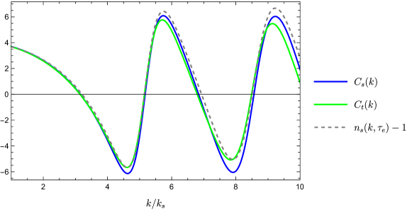
Figure 5: Plot of $C_{s}(k)$, $C_{t}(k)$, and $n_{s}(k,\tau_{e})-1$. We choose $k_{e}/k_{s}=10$ just for illustrative purposes.

One-loop correction (94) can be written as

$$\left\langle\!\left\langle\zeta_{\mathbf{p}}(\tau_{0})\zeta_{-\mathbf{p}}(\tau_{0})\right\rangle\!\right\rangle_{(1)}=\Delta\eta\absolutevalue{\zeta_{p}(\tau_{e})}^{2}\int\frac{\mathrm{d}^{3}k}{(2\pi)^{3}}\left[\frac{1}{2}C_{s}(k)-C_{t}(k)+\frac{1}{4}\Delta\eta\right]\absolutevalue{\zeta_{k}(\tau_{e})}^{2},$$ (95)

where $C_{s}(k)$ is defined in (51) and $C_{t}(k)$ is defined as

$$C_{t}(k)=-4\Delta\eta M_{\mathrm{pl}}^{2}\epsilon(\tau_{s})a^{2}(\tau_{s})\mathrm{Im}\left[\frac{\zeta^{\prime}_{k}(\tau_{e})\zeta_{k}(\tau_{e})}{3k_{e}\absolutevalue{\zeta_{k}(\tau_{e})}^{2}}\zeta_{k}^{*}(\tau_{s})\zeta_{k}^{\prime*}(\tau_{s})\right].$$ (96)

Plot of $C_{t}(k)$ is shown in Fig. 5. For comparison, we also plot $C_{s}(k)$ and $n_{s}(k,\tau_{e})-1$ in the same figure. We can see that $C_{s}(k)\approx C_{t}(k)\approx n_{s}(k,\tau_{e})-1$, so we can approximate the integral as

$$\int\frac{\mathrm{d}^{3}k}{(2\pi)^{3}}\left[\frac{1}{2}C_{s}(k)-C_{t}(k)\right]\absolutevalue{\zeta_{k}(\tau_{e})}^{2} \approx-\frac{1}{2}\int\frac{\mathrm{d}^{3}k}{(2\pi)^{3}}(n_{s}(k,\tau_{e})-1)\absolutevalue{\zeta_{k}(\tau_{e})}^{2}$$

$$=-\frac{1}{2}\int\mathrm{d}\log k~{}\Delta_{s}^{2}(k,\tau_{e})\frac{\mathrm{d}\log\Delta_{s}^{2}(k,\tau_{e})}{\mathrm{d}\log k}\approx-\frac{1}{2}\Delta_{s(\mathrm{PBH})}^{2}.$$ (97)

Then, the one-loop correction becomes

$$\left\langle\!\left\langle\zeta_{\mathbf{p}}(\tau_{0})\zeta_{-\mathbf{p}}(\tau_{0})\right\rangle\!\right\rangle_{(1)}\approx-\frac{1}{2}\Delta\eta\absolutevalue{\zeta_{p}(\tau_{e})}^{2}\Delta_{s(\mathrm{PBH})}^{2}+\frac{1}{4}(\Delta\eta)^{2}\absolutevalue{\zeta_{p}(\tau_{e})}^{2}\int\frac{\mathrm{d}^{3}k}{(2\pi)^{3}}\absolutevalue{\zeta_{k}(\tau_{e})}^{2}.$$ (98)

We compare the one-loop correction to the tree-level contribution as

$$\frac{\left\langle\!\left\langle\zeta_{\mathbf{p}}(\tau_{0})\zeta_{-\mathbf{p}}(\tau_{0})\right\rangle\!\right\rangle_{(1)}}{\left\langle\!\left\langle\zeta_{\mathbf{p}}(\tau_{0})\zeta_{-\mathbf{p}}(\tau_{0})\right\rangle\!\right\rangle_{(0)}}\approx-\frac{1}{2}(\Delta\eta)\Delta_{s(\mathrm{PBH})}^{2}+\frac{1}{4}(\Delta\eta)^{2}\int\frac{\mathrm{d}^{3}k}{(2\pi)^{3}}\absolutevalue{\zeta_{k}(\tau_{e})}^{2}.$$ (99)

In order to trust perturbation theory, this ratio must be much smaller than unity. The first term is one-loop correction predicted by [2]. For $\Delta_{s(\mathrm{PBH})}^{2}\sim 0.1$, the ratio is $\mathcal{O}(0.1)$, so contribution of the first term is quite small . However, there is also the second term. Requiring the second term to be much smaller than unity leads to upper bound $\Delta_{s(\mathrm{PBH})}^{2}\ll\mathcal{O}(0.01)$.

In Eq. (98), we obtain the bare one-loop correction. Issue related to regularization and renormalization is discussed in [1]. Although we focus on SR to USR to SR transition with $\Delta\eta\approx 6$, our result is general for any sharp $\eta$ transition. We briefly discuss other PBH formation models from single-field inflation in [1].

V Conclusion

We have shown that bispectrum in single-field inflation with PBH formation from the USR region satisfies Maldacena’s theorem. At the end of the USR period, the bispectrum is generated by bulk interaction and field redefinition. At the end of inflation, bispectrum is generated only by bulk interaction. We have also demonstrated that the calculation of one-loop correction by source method and direct in-in formalism leads to the same result, confirming our previous conclusion that it is not possible to form appreciable amount of PBHs in single-field inflation.

VI Response to criticism

Our recent letter [1] has been criticized by [2]. In this section, we write our response to that criticism. The author calculates the contribution of the large amplitude of small-scale perturbation to the one-loop correction of the large-scale power spectrum. The author also focuses only on a finite range of momenta that is relevant to PBH formation, so neither infrared (IR) nor ultraviolet (UV) divergence is expected. The author does not perform any regularization or renormalization. The author finds different result of one-loop correction that leads to different conclusion compared to our letter [1].

First, we would like to note that the author of [2] actually finds a similar form of one-loop correction. Based on his Eq. (II.9), the ratio of the one-loop correction to the tree-level contribution is

$$R\equiv\frac{\delta P_{\zeta}(k_{L})}{P_{\zeta}(k_{L})}\sim\Delta\mathcal{P}_{\zeta},$$ (101)

where $\Delta\mathcal{P}_{\zeta}\simeq 0.1$ is peak of small-scale dimensionless power spectrum. Perturbativity at a large scale is violated when $R\simeq 1$. Although the author finds $R\sim 0.1$ without giving the proportionality constant precisely, the author writes “such a correction to be small as well”. At this point, we think it is unclear why the author already expects a small one-loop correction, although the author himself shows that a large amplitude of small-scale perturbation might push the large-scale power spectrum to the limit of perturbativity. Of course, we understand that in the end, the author of [2] finds the proportionality constant is $3/2$ in Eq. (III.23), which would justify his previous speculation, if it were correct.

Now we recall the result of our letter [1]. Compared to Eq. (36) of our letter

$$R\equiv\frac{\Delta_{s(1)}^{2}(p)}{\Delta_{s(\mathrm{SR})}^{2}(p)}=\frac{1}{4}(\Delta\eta)^{2}\left(1.1+\log\frac{k_{e}}{k_{s}}\right)\Delta_{s(\mathrm{PBH})}^{2},$$ (102)

the difference is only in the proportionality constant. We find the proportionality constant is

$$\frac{1}{4}(\Delta\eta)^{2}\left(1.1+\log\frac{k_{e}}{k_{s}}\right)\sim\mathcal{O}(10),$$ (103)

while the author of [2] finds the proportionality constant is $3/2$ that comes from $\Delta\eta/4$. We disagree with it and explain the reason below.

At the end of section III, the author of [2] explains that one-loop correction from the field redefinition $\zeta\rightarrow\zeta_{n}+\eta\zeta_{n}^{2}/4+\zeta_{n}\zeta_{n}^{\prime}$ is suppressed. It means that the one-loop correction that he calculates must only arise from the bulk interaction of $\zeta_{n}$. In particular, action (III.16) should be the action of $\zeta_{n}$, not $\zeta$. Then, the correlation of short modes in the presence of long mode in Eq. (III.22) should also be the correlation of $\zeta_{n}$ evaluated at the end of the USR period. To obtain Eq. (III.23) from Eq. (III.22), the author of [2] takes the same procedure as Eq. (II.9), which is substituting Maldacena’s theorem to Eq. (III.22). We argue that this is incorrect because bispectrum of $\zeta_{n}$ at the end of USR period does not satisfy the theorem, as we explained in § III.1 to § III.3 of this paper. We have derived the one-loop correction from bispectrum in § IV.1 of this paper based on the same method adopted in [2]. After correcting the error of [2], we obtained the same result compared to direct in-in formalism in § IV.2.

In summary, the author of [2] incorrectly substituted Maldacena’s theorem for the bispectrum that is generated only by bulk interaction at the end of the USR period. This has led to incorrect one-loop correction results. After fixing such a mistake, we have shown that the one-loop correction in our letter based on the in-in formalism [1] is reproduced even in the method employed in [2].