A Practical Upper Bound for the Worst-Case Attribution Deviations

Abstract

Model attribution is a critical component of deep neural networks (DNNs) for its interpretability to complex models. Recent studies bring up attention to the security of attribution methods as they are vulnerable to attribution attacks that generate similar images with dramatically different attributions. Existing works have been investigating empirically improving the robustness of DNNs against those attacks; however, none of them explicitly quantifies the actual deviations of attributions. In this work, for the first time, a constrained optimization problem is formulated to derive an upper bound that measures the largest dissimilarity of attributions after the samples are perturbed by any noises within a certain region while the classification results remain the same. Based on the formulation, different practical approaches are introduced to bound the attributions above using Euclidean distance and cosine similarity under both $\ell_{2}$ and $\ell_{\infty}$-norm perturbations constraints. The bounds developed by our theoretical study are validated on various datasets and two different types of attacks (PGD attack and IFIA attribution attack). Over 10 million attacks in the experiments indicate that the proposed upper bounds effectively quantify the robustness of models based on the worst-case attribution dissimilarities.

1 Introduction

Attribution methods play an important role in deep learning applications as one of the subareas of explainable AI. Practitioners use attribution methods to measure the relative importance among different features and to understand the impacts of features contributing to the model outputs. They have been widely used in a number of critical real-world applications, such as risk management [2], medical imaging [24, 29] and drug discovery [13]. In particular, attributions are supposed to be secure and resistant to external manipulation such that proper explanations can be applied to safety-sensitive applications. Regulations are also deployed in countries to enforce the interpretability of deep learning models for a ‘right to explain’ [10]. Although attribution methods have been extensively studied [28, 36, 18, 25, 31, 39], recent works reveal that they are vulnerable to visually imperceptible perturbations that drastically alter the attributions and keep the model outputs unchanged [8, 6].

Prior works [4, 3, 12, 30, 33, 23, 32] investigate the attribution robustness based on empirical and statistical estimations over entire dataset. However, current attribution robustness works are unable to evaluate how robust the model is given any arbitrary test point, perturbed or unperturbed. In this paper, we study the problem of finding the worst attribution perturbation within certain predefined regions. Specifically, given a trained model and an image sample, we propose theoretical upper bounds of the attribution deviations from the unperturbed ones. As far as we know, this is the first attempt to provide an upper bound of attribution differences.

In this paper, the general upper bound for attribution deviation is first quantified as the maximum changes of attributions after the samples are perturbed while classification results remain the same. Two cases are analyzed, including with and without label constraint, which refers to the classification labels being unchanged and changed, respectively, after the original samples are attacked. For each case, two mostly used perturbation constraints, $\ell_{2}$ and $\ell_{\infty}$-norm, are considered to compute the upper bound. For $\ell_{2}$-norm constraint, our approach is based on the first-order Taylor series of model attribution, and a tight upper bound ignoring the label constraint is computed from the singular value of the attribution gradient. $\ell_{\infty}$-norm constraint is more complicated because the upper bound is a solution of a concave quadratic programming with box constraints, which is an NP-hard problem. Thus, two relaxation approaches are proposed. Moreover, a more restricted bound constrained on the unchanged label is also studied. In this study, Euclidean distance and cosine distance, which are also employed in the previous empirical studies [4, 30, 32], are used as dissimilarity functions to measure attribution difference. We summarize the contributions of this paper as follows:

• We formally define the general upper bound for attribution deviation as the optimization problem with norm constraint and label constraint to find the maximum change of attributions after samples being attacked. According to the best knowledge of the authors, it has not been studied before.

• The tight upper bounds for $\ell_{2}$-norm constrained attacks with and without classification label constraints are proposed based on the first-order Taylor series. The proposed bound without label constraints generalizes to all gradient-based attribution methods, and the one with label constraints is applicable to all attribution methods satisfying the axiom of completeness.

• Two different approaches are provided to bound the $\ell_{\infty}$-norm constrained attacks above, which uses an $\ell_{p}$-norm relaxation and a mathematical property of the quadratic form.

• The experimental results show that the upper bounds derived in this paper can effectively bound the attribution differences between all 10 million attacked samples and their corresponding original samples from different models, datasets, attack methods and parameters choices.

The rest of this paper is organized as follows. We start with an introduction to notations and related works. The formulation of the general upper bound for attribution deviation is defined in Sec. 3. Specific methods to find the upper bounds in different scenarios are provided in Sec. 4. In Sec. 5, detailed experimental results are presented and the paper concludes in Sec. 6.

2 Preliminaries and related works

We consider a twice-differentiable classifier $f$ that maps the input set $\mathcal{D}=\left\{({\bm{x}}^{(i)},y^{(i)})\right\}_{i=1}^{n}$ to the logits, $f:\mathbb{R}^{d}\rightarrow\mathbb{R}^{k}$, where ${\bm{x}}^{(i)}\in\mathbb{R}^{d}$ and $y^{(i)}\in\left\{1,\ldots,k\right\}$ represent the $i$-th sample and its ground truth label. The non-bold version $x_{k}$ represents the $k$-th feature of ${\bm{x}}$ and $f_{y}$ is the logit at label $y$. The model attribution of the input sample given label $y$ is computed by $g^{y}:\mathbb{R}^{d}\rightarrow\mathbb{R}^{d}$, and we denote the attribution of ${\bm{x}}$ by $g^{y}({\bm{x}})$.

2.1 Model attribution

The model attribution studies the importance of each input feature $x_{i}$ that contributes to the final output $f_{y}({\bm{x}})$. We can classify the most used attribution methods into two categories, perturbations-based methods [36, 39] and backpropagation-based methods [25, 1], which include gradient-based methods. In particular, in this paper, we focus on the most commonly used gradient-based attribution methods, saliency map (SM), gradient*input and integrated gradient (IG). Saliency map [28] is defined as the gradients of output with respect to the input. Gradient*input [26] is computed by element-wise multiplication of input features and the gradients. Integrated gradients [31] is defined as line integral of gradients from a baseline image $\bm{a}$ to the input image ${\bm{x}}$ weighted by their difference. It is worth noting that IG satisfies the axiom of completeness, $\sum_{i}g_{i}^{y}({\bm{x}})=f_{y}({\bm{x}})$, which builds a direct connection between the attributions and model outputs. The mathematical expressions and examples of the attribution methods are given in Table 1.

Table 1: Mathematical expressions and visual examples of the selected attribution methods. Attributions have been taken absolute values and are presented heatmaps to reflect relative importance among pixels. The baseline $\bm{a}$ of IG is chosen as a black image. $\otimes$ denotes the element-wise multiplication.

Original image	Saliency map	Input*gradient	Integrated gradients
	$\nabla f_{y}({\bm{x}})$	${\bm{x}}\otimes\nabla f_{y}({\bm{x}})$	$({\bm{x}}-\bm{a})\otimes\int_{0}^{1}\nabla f_{y}(\bm{a}+\alpha({\bm{x}}-\bm{a}))\,d\alpha$

2.2 Attribution robustness

It has been discovered in the literature that model attributions can be easily sabotaged by adversaries. Similar to adversarial examples [9], human-indistinguishable perturbations can be also augmented to natural images that, though classification results remain unchanged, misdirect the model attributions towards meaningless interpretations [8] or any predefined arbitrary patterns which are unrelated to the original images [6].

To mitigate the threat of being attacked, researchers have also worked on training attribution robust models. The most considered techniques are adapted from adversarial training [19], and they minimize the differences between original and the worst-case perturbed attributions. Boopathy et al. [3] and Chen et al. [4] consider the $\ell_{1}$-norm distance to measure the difference between attributions, and Ivankay et al. [12] uses Pearson correlation coefficient. Singh et al. [30] and Wang et al. [33] choose $\ell_{2}$-norm distance, where the former minimizes the spatial correlation between image and attribution using a soft-margin triplet loss, and the latter shows the smoothness of the decision surface is related to attribution robustness based on a geometric understanding. Wang & Kong [32] emphasizes the directions of attributions using the relationship between Kendall’s rank correlation and cosine similarity and protects the attribution based on the latter. However, none of the aforementioned methods defines a quantitative measurement to the attribution changes after perturbation. More clearly, the attributions are not guaranteed to be protected for all perturbations within the allowable region that do not alter the classification outputs.

3 Formulation of general upper bound for attribution deviations

In this section, we formally define the general upper bound for attribution deviation as a measurement of attribution robustness. Recall that adversaries incapacitate the attributions of neural networks by adding imperceptible noises to natural images. For an attributional robust model, on the contrary, the imperceptible noises should not change the interpretability of attributions, i.e., images perturbed by noises should provide similar attributions as the original ones. To evaluate such resistance against adversaries, it is essential to find an upper bound that represents the worst-case dissimilarity of attributions after the original images being perturbed. Thus, we define the general upper bound for attribution deviations as follows.

Definition 1 (General upper bound for attribution deviations).

Given a trained neural network $f$, a fixed allowable region for perturbation $\bm{\delta}$, $\mathcal{B}_{\varepsilon}=\left\{\bm{\delta}:\|\bm{\delta}\|_{p}\leq\varepsilon\right\}$, and an input sample ${\bm{x}}$, the general upper bound for attribution deviations $T(\varepsilon;{\bm{x}})$ is defined that, for all perturbations $\bm{\delta}\in\mathcal{B}_{\varepsilon}$, if $\operatorname*{arg\,max}_{k}f_{k}({\bm{x}})=\operatorname*{arg\,max}_{k}f_{k}({\bm{x}}+\bm{\delta})$, then their corresponding attributions satisfy that $D(g^{y}({\bm{x}}),g^{y}({\bm{x}}+\bm{\delta}))\leq T(\varepsilon;{\bm{x}})$.

In the above definition, $D(\cdot,\cdot)$ is a dissimilarity metric that measures the difference between two attributions, where a smaller value indicates that two attributions are more similar and represent closer meaningful interpretations. $T$ is a function with respect to the threshold $\varepsilon$ and ${\bm{x}}$. The definition formalizes the guarantee of attribution robustness, where when the model is more robust, the model attributions being attacked are less likely to be misled. More precisely, when being attacked, the change of attribution is bounded above and the smaller upper bound indicates the more attributional robust model.

Based on the above definition, the general upper bound for attribution deviations $T(\varepsilon;{\bm{x}})$ can be found by solving the following optimization problem

$$\max_{\bm{\delta}} D(g^{y}({\bm{x}}),g^{y}({\bm{x}}+\bm{\delta}))$$ (1)

s.t. $$\|\bm{\delta}\|_{p}\leq\varepsilon$$

$$\operatorname*{arg\,max}_{k}f_{k}({\bm{x}})=\operatorname*{arg\,max}_{k}f_{k}({\bm{x}}+\bm{\delta})$$

We refer the first constraint $\|\bm{\delta}\|_{p}\leq\varepsilon$ to the norm constraint and the second one to the label constraint as it requires the unchanged label after being perturbed. In following sections, we attempt to solve the optimization problem (1) using the two mostly used norm constraints on the perturbations, $\ell_{2}$ and $\ell_{\infty}$, i.e., $\|\bm{\delta}\|_{2}\leq\varepsilon$ and $\|\bm{\delta}\|_{\infty}\leq\varepsilon$. For the dissimilarity metric, we choose from previously used attribution measurements, the Euclidean distance and the cosine distance. An alternative formulation of this problem is to find the maximum perturbation $\varepsilon$ subject to $D(g^{y}({\bm{x}}),g^{y}({\bm{x}}+\bm{\delta}))\leq\omega$ where $\omega$ is a predefined threshold. The results obtained from problem (1) can be converted directly to the alternative formulation, and we defer the procedures to Appendix E.

4 A practical upper bound for attribution deviations

4.1 Upper bound under $\ell_{2}$-norm constraint without the label constraint

To start with, the upper bound without label constraints is studied. This will provide a looser bound since, intuitively, stronger adversaries are allowed to perturb the samples that may change the classification results. While perturbations are restricted in a small region and indistinguishable to human, they could be enough to cause huge difference in attributions. The upper bound for $\ell_{2}$-norm constrained case is a straightforward derivation of the first-order Taylor series of attribution functions. The following theorem provides a tight bound for attribution robustness assuming that the attribution function is locally linear.

Theorem 1.

Given a twice-differentiable classifier $f:\mathbb{R}^{d}\rightarrow\mathbb{R}^{k}$, and its attribution $g^{y}$ on label $y$, assume that $g^{y}$ is locally linear within the neighborhood of ${\bm{x}}$, $\mathcal{B}_{\varepsilon}({\bm{x}})=\left\{{\bm{x}}+\bm{\delta}|\|\bm{\delta}\|_{2}\leq\varepsilon\right\}$, then for all perturbations $\|\bm{\delta}\|_{2}\leq\varepsilon$,

$$\|g^{y}({\bm{x}}+\bm{\delta})-g^{y}({\bm{x}})\|_{2}\leq\xi_{max}\varepsilon,$$

where $\xi_{max}$ is the largest singular value of $H=\nabla g^{y}({\bm{x}})$.

Proof.

Based on the Taylor series of $g^{y}({\bm{x}})$ and the above condition, we have

$$\|g^{y}({\bm{x}}+\bm{\delta})-g^{y}({\bm{x}})\|_{2}^{2} \leq\|\bm{\delta}^{\top}\nabla g^{y}({\bm{x}})\|_{2}^{2}$$ (2)

$$=\bm{\delta}^{\top}\nabla g^{y}({\bm{x}})\nabla g^{y}({\bm{x}})^{\top}\bm{\delta}$$ (3)

$$=\frac{\bm{\delta}^{\top}}{\|\bm{\delta}\|_{2}}P\frac{\bm{\delta}}{\|\bm{\delta}\|_{2}}\cdot\|\bm{\delta}\|^{2}_{2}$$ (4)

$$\leq\lambda_{max}\|\bm{\delta}\|^{2}_{2}\leq\lambda_{max}\varepsilon^{2}$$ (5)

where $\lambda_{max}$ is the largest eigenvalue of $P=HH^{\top}=\nabla g^{y}({\bm{x}})\nabla g^{y}({\bm{x}})^{\top}$, and $\bm{v}_{max}$ is the corresponding eigenvector. The equality in Eq. (5) is achieved when $\bm{\delta}$ is $\varepsilon\bm{v}_{max}$ or $-\varepsilon\bm{v}_{max}$. Since the singular values of $H$ are equal to the square root of the eigenvalues of $P$, then,

$$\|g^{y}({\bm{x}}+\bm{\delta})-g^{y}({\bm{x}})\|_{2}\leq\sqrt{\lambda_{max}}\varepsilon=\xi_{max}\varepsilon.$$ (6)

∎

Note that the local linearity of attribution function is a weak assumption for both attribution and adversarial robust models since most of the defense methods [22, 33] attempt to smoothen the functions. In addition, when the magnitude of perturbation $\bm{\delta}$ is constrained to small size, the magnitude of the higher-order Taylor remainders is negligible. We include the empirical results evaluating this assumption in Appendix B. Furthermore, we also provide a generalization of the theorem that bounds the attribution differences as a function of a constant $c\geq 1$ that measures the error margin of the first-order Taylor series in Appendix B.2, which can be applied similarly to all other results in this work.

It is also noticed that the above theorem uses the gradient of attribution $H=\nabla g^{y}({\bm{x}})$, which is also the Hessian matrix $\nabla^{2}f_{y}({\bm{x}})$ when the attribution is chosen as saliency maps and can be computed easily for other gradient-based attribution methods. Moreover, the second-order derivatives can be zeros for ReLU networks [6]. In this work, the non-linearity functions are replaced by softplus function $f({\bm{x}};\beta)=\frac{1}{\beta}\log(1+e^{\beta{\bm{x}}})$ as in Dombrowski et al. [6]. A 2D example of the upper bound is illustrated in Fig. 1(a). The optimum solution is in the same direction as the semi-major axis of the ellipse, which represents $\bm{\delta}^{\top}P\bm{\delta}$. The circle represents the 2D Euclidean ball bounded by $T(\varepsilon;{\bm{x}})$, which is derived from the length of the semi-major axis.

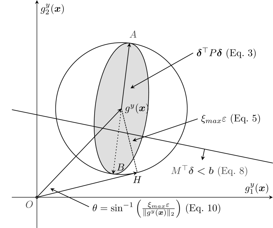
(a)

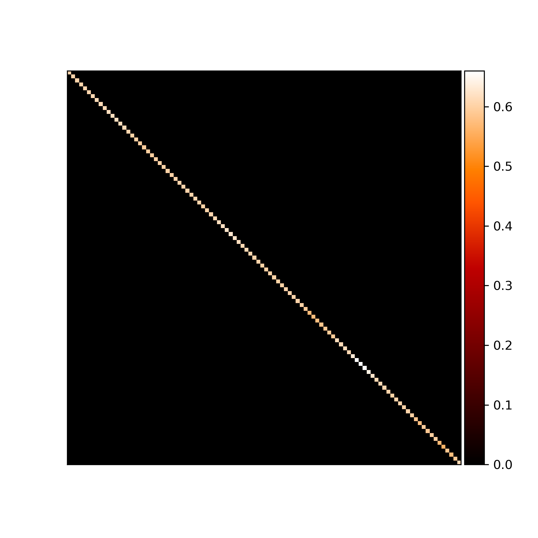
(b)

Figure 1: (a) 2D illustration of the proposed upper bound on Euclidean distance and cosine distance. (b) Visualization of the absolute values of gradient IG as a heat map. The gradient is generated using CIFAR-10 ($3072\times 3072$), and the values are normalized to $[0,1]$. Here the first 100 dimensions of each axis are plotted for better visualization. More figures and the mathematical analysis are given in Appendix C.

4.2 Upper bound under $\ell_{\infty}$-norm constraint without the label constraint

The upper bound for $\ell_{\infty}$-norm constrained case is more complicated as $\|\bm{\delta}\|_{\infty}\leq\varepsilon$ defines a box constraints inequality system that $-\varepsilon\leq\delta_{i}\leq\varepsilon$ for all $i$. If we still consider the quadratic form derived from the first-order Taylor series as in Sec. 4.1, the above optimization problem (1) turns into a concave quadratic programming with box constraints, which is NP-hard [21]. In order to compute the upper bound efficiently, we consider a loose relaxation of $p$-norms.

Corollary 1.

Given a twice-differentiable classifier $f:\mathbb{R}^{d}\rightarrow\mathbb{R}^{k}$, and its attribution $g^{y}$ on label $y$, assume that $g^{y}$ is locally linear within the neighborhood of ${\bm{x}}$, $\mathcal{B}_{\varepsilon}({\bm{x}})=\left\{{\bm{x}}+\bm{\delta}|\|\bm{\delta}\|_{p}\leq\varepsilon\right\}$, then for all perturbations $\|\bm{\delta}\|_{p}\leq\varepsilon$ that $p>2$, $\|g^{y}({\bm{x}}+\bm{\delta})-g^{y}({\bm{x}})\|_{2}\leq d^{\frac{1}{2}-\frac{1}{p}}\xi_{max}\varepsilon$, where $\xi_{max}$ is the largest singular value of $H=\nabla g^{y}({\bm{x}})$.

The proof of the relaxation of $p$-norm and Corollary 1 can be found in Appendix A.1. Note that this corollary not only avoids the NP-hard problem for $\ell_{\infty}$-norm constraint, but it is also a general upper bound for $p$-norm constraint on $\bm{\delta}$ for all $p>2$. However, it is also noticed that the upper bound increases with respect to the input sample dimension. The multiplication factor for $\ell_{\infty}$ is $\sqrt{d}$. For high-dimensional input samples, the provided method would scale up to an extremely loose upper bound that can be trivial but meaningless. To better bound the attribution deviations in the $\ell_{\infty}$-norm case, we provide a tighter upper bound using the sparsity of attribution gradients.

Theorem 2.

Given a twice-differentiable classifier $f$, its attribution on label $y$, $g^{y}$, and the gradient $H=\nabla g^{y}$, assume that $g^{y}$ is locally linear within the neighborhood of ${\bm{x}}$, $\mathcal{B}_{\varepsilon}({\bm{x}})=\left\{{\bm{x}}+\bm{\delta}|\|\bm{\delta}\|_{\infty}\leq\varepsilon\right\}$, then for all perturbations $\|\bm{\delta}\|_{\infty}\leq\varepsilon$,

$$\|g^{y}({\bm{x}}+\bm{\delta})-g^{y}({\bm{x}})\|_{2}\leq\varepsilon\sqrt{\sum_{i,j}\left|P_{ij}\right|}.$$ (7)

where $P=HH^{\top}$ and the equality is taken at $\bm{\delta}=(\pm\varepsilon,\ldots,\pm\varepsilon)^{\top}$.

The proof is deferred to Appendix A.2. This upper bound as the summation of absolute values of the matrix $P=\nabla g^{y}({\bm{x}})\nabla g^{y}({\bm{x}})^{\top}$ is shown to be tighter than that given in Corollary 1 since $P$ is a diagonal-dominated and positive semi-definite matrix (see Fig. 1(b)), which implies that $\left|P_{ii}\right|\approx\lambda_{i}$.

4.3 Upper bound with the label constraint

In this section, we extend our study of the upper bound to the case that labels are not changed after the samples are perturbed. Here, only attribution methods satisfying the axiom of completeness are studied as the axiom provides a direct connection between attributions and model outputs, i.e., $\sum_{i}g_{i}^{y}({\bm{x}})=f_{y}({\bm{x}})$. The following proposition gives a sufficient condition to ensure that the classification result remains unchanged after the sample is perturbed.

Proposition 1.

Denote the gradient-based attribution satisfying the completeness axiom of ${\bm{x}}$ on ground truth label $y$ by $g^{y}({\bm{x}})$, and the attribution on a different label $y^{\prime}$ by $g^{y^{\prime}}({\bm{x}})$. Given the perturbation $\bm{\delta}$, assume that $g^{y}$ is locally linear within the neighborhood of ${\bm{x}}$, $\mathcal{B}_{\varepsilon}({\bm{x}})=\left\{{\bm{x}}+\bm{\delta}|\|\bm{\delta}\|_{p}\leq\varepsilon\right\}$, the classification result of ${\bm{x}}+\bm{\delta}$ does not change from $y$ to $y^{\prime}$ if

$$\left(\left(\nabla g^{y^{\prime}}({\bm{x}})-\nabla g^{y}({\bm{x}})\right)\Delta\right)^{\top}\bm{\delta}<f_{y}({\bm{x}})-f_{y^{\prime}}({\bm{x}}),$$ (8)

where $\Delta$ is an all one vector, $\Delta=\left(1,\ldots,1\right)^{\top}\in\mathbb{R}^{d}$.

The full proof can be found in Appendix A.3. Note that the inequality is linear to $\bm{\delta}$ and we denote $M=(\nabla g^{y^{\prime}}({\bm{x}})-\nabla g^{y}({\bm{x}}))\Delta$ and $b=f_{y}({\bm{x}})-f_{y^{\prime}}({\bm{x}})$ for simplicity, i.e., $M^{\top}\bm{\delta}<b$. To bound the attribution differences after the sample is perturbed by noise $\bm{\delta}$ in $\ell_{2}$-norm ball, i.e., $\|\bm{\delta}\|_{2}\leq\varepsilon$, the upper bound can be formulated by rewriting the optimization problem (1) as the optimal value of the following quadratic programing with concave objective function and a system of linear constraints for all labels different from $y$,

$$\max_{\bm{\delta}}~{}\bm{\delta}^{\top}P\bm{\delta}\quad\text{s.t. }\|\bm{\delta}\|_{2}\leq\varepsilon\text{ and }M^{\top}\bm{\delta}<b.$$ (9)

To simplify the computation, in this work, we only consider the second best label $y^{\prime}$, i.e., $y^{\prime}=\operatorname*{arg\,max}_{k\in\left\{1,\ldots,c\right\}\backslash y}f_{k}({\bm{x}})$. In such case, the constraint $M^{\top}\bm{\delta}<b$ defines a half-space. Recall that Theorem 1 states that the upper bound in $\ell_{2}$-norm case without label constraint is $\xi_{max}\varepsilon$, and we noticed that this bound is achieved at two opposite vectors $\bm{\delta}^{\ast}=\varepsilon\bm{v}_{max}$ or $\bm{\delta}^{\ast}=-\varepsilon\bm{v}_{max}$. Thus, at least one of these two vectors lies in the half-space defined by the linear constraint (see point $A$ and $B$ in Fig. 1(a). Therefore, the upper bound provided in Theorem 1 is also achieved even if the label constraint is added, i.e., the optimal value of optimization problem (9) is also $\xi_{max}\varepsilon$.

The bound of $\ell_{p}$-norm constrained case can be derived similarly. The less tight upper bound is still achievable at $d^{\frac{1}{2}-\frac{1}{p}}\xi_{max}\varepsilon$ as in Corollary 1. Generalizing the $\ell_{\infty}$-norm constrained upper bound using Eq. 7 is simpler. According to Theorem 2, there are $2^{d}$ different optimal solutions that achieve the optimum and they are the corners of the $\ell_{\infty}$-norm box. As long as the feasible region is non-empty, there exists at least one corner of the box lying inside the feasible region, and the optimum value is achieved. Similarly, given a $d$-dimensional $\ell_{\infty}$-norm box, and $k$ label constraints that each separates the entire space into two half-spaces, if at least one corner of the box lies within the feasible region, the optimum value is attainable.

4.4 Upper bound based on cosine distance

In the previous parts of this section, we discussed several practical upper bounds based on Euclidean distance. It is noticed that Wang & Kong [32] claims that cosine similarity ($D_{s}$) is a better metric to measure the difference of attributions as it emphasizes the relative importance among different features rather than the absolute magnitude of each individual feature. Our method can be trivially extended to the scenarios using cosine distance ($D_{c}=1-D_{s}(g^{y}({\bm{x}}+\bm{\delta}),g^{y}({\bm{x}}))$) as the dissimilarity function $D$ defined in the formulation (1) with simple modifications.

Corollary 2.

Given a twice-differentiable classifier $f:\mathbb{R}^{d}\rightarrow\mathbb{R}^{k}$ and its attribution $g^{y}$ on label $y$, for all perturbations $\|\bm{\delta}\|_{p}\leq\varepsilon$, if the Euclidean distance of $g^{y}({\bm{x}}+\bm{\delta})$ and $g^{y}({\bm{x}})$ is upper bounded by $T(\varepsilon;{\bm{x}})$, and $0\leq T(\varepsilon;{\bm{x}})\leq\|g^{y}({\bm{x}})\|_{2}$, then their cosine distance ($D_{c}$) is upper bounded by

$$D_{c}(g^{y}({\bm{x}}+\bm{\delta}),g^{y}({\bm{x}}))\leq 1-\sqrt{1-\frac{T(\varepsilon;{\bm{x}})^{2}}{\|g^{y}({\bm{x}})\|^{2}_{2}}}.$$ (10)

This upper bound is valid when the assumption that $0\leq T(\varepsilon;{\bm{x}})\leq\|g^{y}({\bm{x}})\|_{2}$ is satisfied, i.e., the variation of attribution distance is smaller than the original attribution. As shown in Fig. 1(a), the angle between original and perturbed attributions is bounded by $\theta$ computed from the corollary.

5 Experimental results

Table 2: Evaluation of upper bound without the label constraint.

	SM					Input*gradient					IG
	$\widehat{T}_{e}$	$T_{e}$	$T^{\prime}_{e}$	$\widehat{T}_{c}$	$T_{c}$	$\widehat{T}_{e}$	$T_{e}$	$T^{\prime}_{e}$	$\widehat{T}_{c}$	$T_{c}$	$\widehat{T}_{e}$	$T_{e}$	$T^{\prime}_{e}$	$\widehat{T}_{c}$	$T_{c}$
$\ell_{2}$	0.09	0.31	0.34	6.88	7.41	0.07	0.46	0.46	0.51	2.60	0.02	0.17	0.17	1.80	3.84
$\ell_{\infty}$	0.41	0.85	-	21.87	27.09	0.07	0.69	-	7.03	50.59	0.25	0.52	-	23.24	35.00

In this section, we evaluate the effectiveness of proposed upper bounds by numerical experiments under both $\ell_{2}$ and $\ell_{\infty}$-norms. In the following results, we compute the theoretical upper bounds for adversarial robust models and attributional robust models, including Adversarial Training (AT) [19], IG-NORM [4], Adversarial Attributional Training with robust training loss (AdvAAT) [12], Attributional Robustness Training (ART) [30], TRADES [37] and Integrated Gradients Regularizer (IGR) [32]. We follow previous attribution robustness studies to use ResNet-18 to evaluate CIFAR-10 [15], and use the neural network with four convolutional layers followed by three fully-connected layers to evaluate MNIST [17] and Fashion-MNIST [34]. The proposed upper bounds are also scalable to datasets with larger images, but due to the scalability problem of existing attribution defense methods, we provide evaluations of Flower [20] and ImageNet [5] on attributional non-robust models in Appendix D.3.

For each selected model, the theoretical upper bounds for both Euclidean distance and cosine distance are computed. We convert the cosine values to degrees for easier comparison. The theoretical bounds are compared with corresponding distance between original sample and attacked sample to verify the effectiveness of the bounds. We denote the theoretical upper bounds for Euclidean distance and cosine distance as $T_{e}$ and $T_{c}$, respectively. The $\ell_{2}$ PGD-20 attack [19] is implemented for $\ell_{2}$-norm bounded case. The 200-step IFIA with the top-$k$ intersection as dissimilarity function [8] is implemented for $\ell_{\infty}$-norm bounded case, where $k$ is 100 for MNIST and Fashion-MNIST and 1000 for CIFAR-10. Each sample is attacked 20 times and the mean distance is computed. The sample mean Euclidean and cosine distances of the entire dataset under corresponding attacks are denoted by $\widehat{T}_{e}$ and $\widehat{T}_{c}$, respectively. All the experiments are implemented on NVIDIA GeForce RTX 3090 .

In addition, we also provide a generalization of the proposed bounds based on the generalization of Theorem 1 (Appendix B.2) that adaptively multiply a scalar $c$ for an given input ${\bm{x}}$ in case that the weak assumption is violated in rare cases. Explicitly, the adaptive value of $c$ for $i$-th sample is given as follows (details in Appendix B.3)

$$c^{(i)}=\max\left\{1,\frac{\|g^{y}({\bm{x}}^{(i)}+\varepsilon\bm{v}^{(i)}_{max})-g^{y}({\bm{x}}^{(i)})\|_{2}}{\xi^{(i)}_{max}\varepsilon}\right\}.$$ (11)

5.1 Evaluation of upper bounds without the label constraint

We first evaluate the upper bounds without label constraints, which can be applied to any gradient-based attribution method. Here three methods are evaluated, saliency map, input*gradient and integrated gradients. The upper bounds computed from TRADES+IGR on CIFAR-10 are presented in Table 2, and results from other models are deferred to Appendix D.1. We use the unlabelled upper bound introduced in Theorem 1 and 2 to compute $T_{e}=\xi_{max}\varepsilon$ and extend it to $T_{c}$ using Eq. 10. The perturbation size is chosen to be 0.1 for $\ell_{2}$ and 0.25 for $\ell_{\infty}$. The generalized upper bound $T^{\prime}_{e}=c\xi_{max}\varepsilon$ (Eq. 11) is also provided for $\ell_{2}$ case, and is not necessary for $\ell_{\infty}$ case. As observed in the table, the proposed upper bounds are valid for different attribution methods and both Euclidean and cosine distances are well-bounded. More precisely, none of the $\ell_{\infty}$ perturbed attributions is outside the theoretical bound and none of the $\ell_{2}$ perturbed attributions is outside the generalized bound.

5.2 Evaluation of upper bounds under $\ell_{2}$-norm constraint and label constraint

To evaluate the upper bound of attribution deviations after samples being attacked by $\ell_{2}$-norm constrained perturbations, we use the method provided in Sec. 4.3 and 4.4 to obtain the theoretical upper bounds for both Euclidean distance ($T_{e}=\xi_{max}\varepsilon$) and cosine distance ($T_{c}$ in Eq. 10). Integrated gradients (IG) is chosen here as the theoretical bound with the label constraint is based on the axiom of completeness. Besides, as discussed in Sec. 4.1, the percentages of attacked attribution outside $T_{e}$ are provided, and the generalized bound is also calculated and denoted by $T^{\prime}_{e}=c\xi_{max}\varepsilon$. Since $T^{\prime}_{e}$ bounds all the attacked attributions, i.e., 100% for all the models, we do not report the percentages in the table. From Table 3, we observe the following results. (i) The percentages are low, which supports our assumption in Sec. 4.1 that $g^{y}$ is locally linear. (ii) The computed values for both Euclidean ($T^{\prime}_{e}$) and cosine distance ($T_{c}$) successfully bound the attribution differences above for every dataset and every model. In addition, we also show the minimum Euclidean gaps between samples and bounds in Section 5.4 to illustrate that the tightness of the proposed bounds.

Table 3: Evaluation of upper bounds under $\ell_{2}$-norm constraint and label constraint. The numbers in the brackets indicate the percentages that attacked attribution is outside the $T_{e}$.

Model	$\widehat{T}_{e}$	$T_{e}$	$T^{\prime}_{e}$	$\widehat{T}_{c}$($\deg$)	$T_{c}$($\deg$)
$\varepsilon=0.05$	MNIST
AT	0.0685	0.1537 [2.25%]	0.1596	3.6935	7.0951
IG-NORM	0.1158	0.2888 [2.00%]	0.2967	3.3174	7.2615
ART	0.0626	0.3591 [6.00%]	0.3702	2.3923	6.8657
AdvAAT	0.0876	0.3269 [6.20%]	0.3404	1.9034	6.8992
TRADES	0.1620	0.5060 [1.68%]	0.5271	2.8374	6.9988
TRADES+IGR	0.1784	0.4964 [1.32%]	0.5145	2.9075	6.9779
$\varepsilon=0.05$	Fashion-MNIST
AT	0.0659	0.0700 [2.19%]	0.0869	10.1442	12.9577
IG-NORM	0.1181	0.1789 [0.00%]	0.1789	6.6002	8.8043
AdvAAT	0.1115	0.1735 [6.20%]	0.1858	5.8544	9.3692
ART	0.0940	0.1387 [0.94%]	0.1411	5.4507	9.8234
TRADES	0.0626	0.0963 [4.16%]	0.1184	8.3521	12.0991
TRADES+IGR	0.0403	0.0453 [1.91%]	0.0507	7.7302	8.8411
$\varepsilon=0.1$	CIFAR-10
AT	0.0392	0.2532 [0.09%]	0.2533	2.7335	4.7724
IG-NORM	0.0149	0.1582 [0.42%]	0.1621	1.6505	4.3711
AdvAAT	0.0374	0.2386 [0.06%]	0.2386	0.2847	3.8202
ART	0.0733	0.2278 [0.00%]	0.2278	0.5918	4.2123
TRADES	0.0264	0.1734 [0.16%]	0.1734	1.9084	3.8686
TRADES+IGR	0.0240	0.1692 [0.09%]	0.1692	1.8011	3.8384

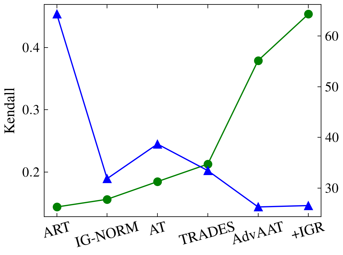
(a) MNIST

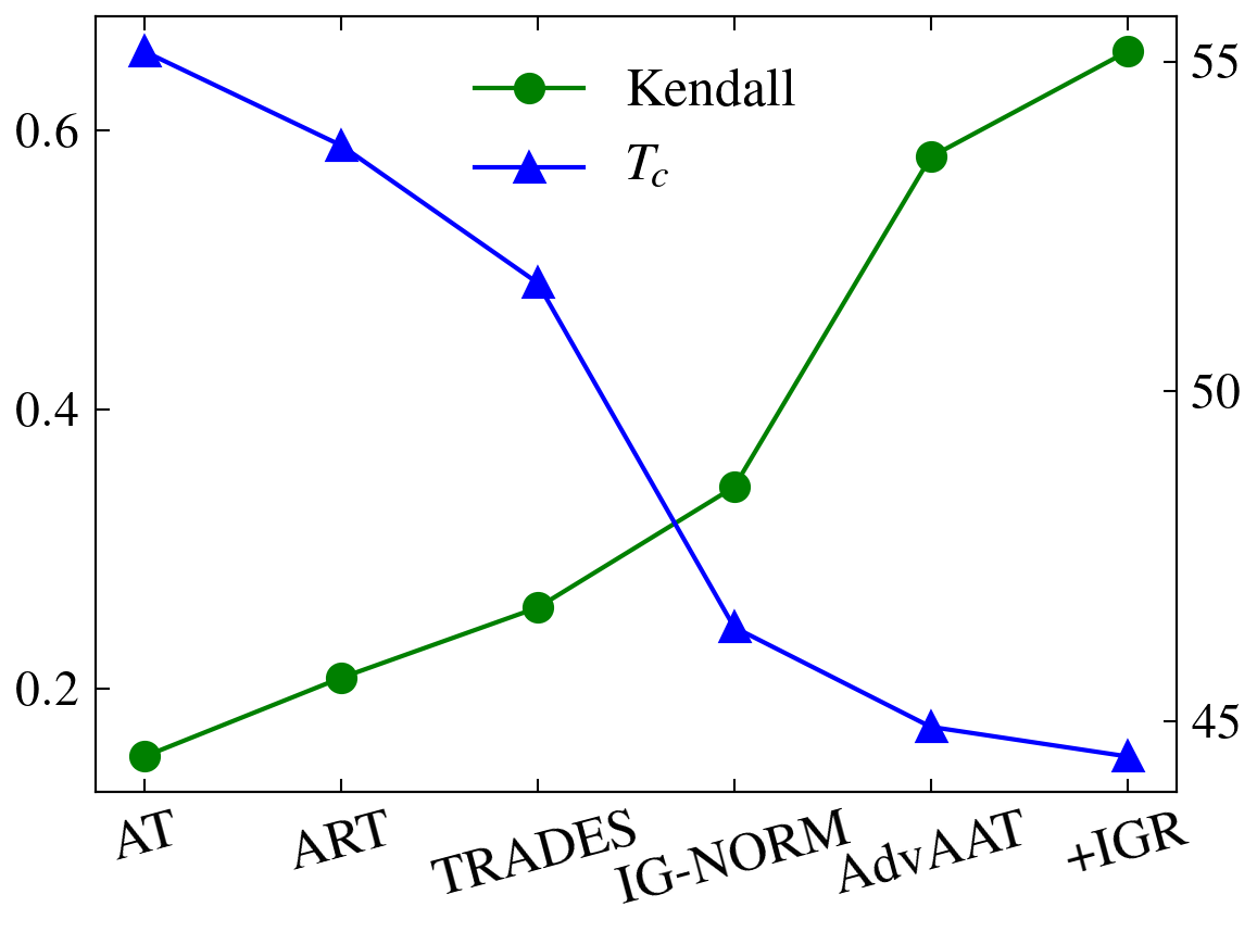
(b) Fashion-MNIST

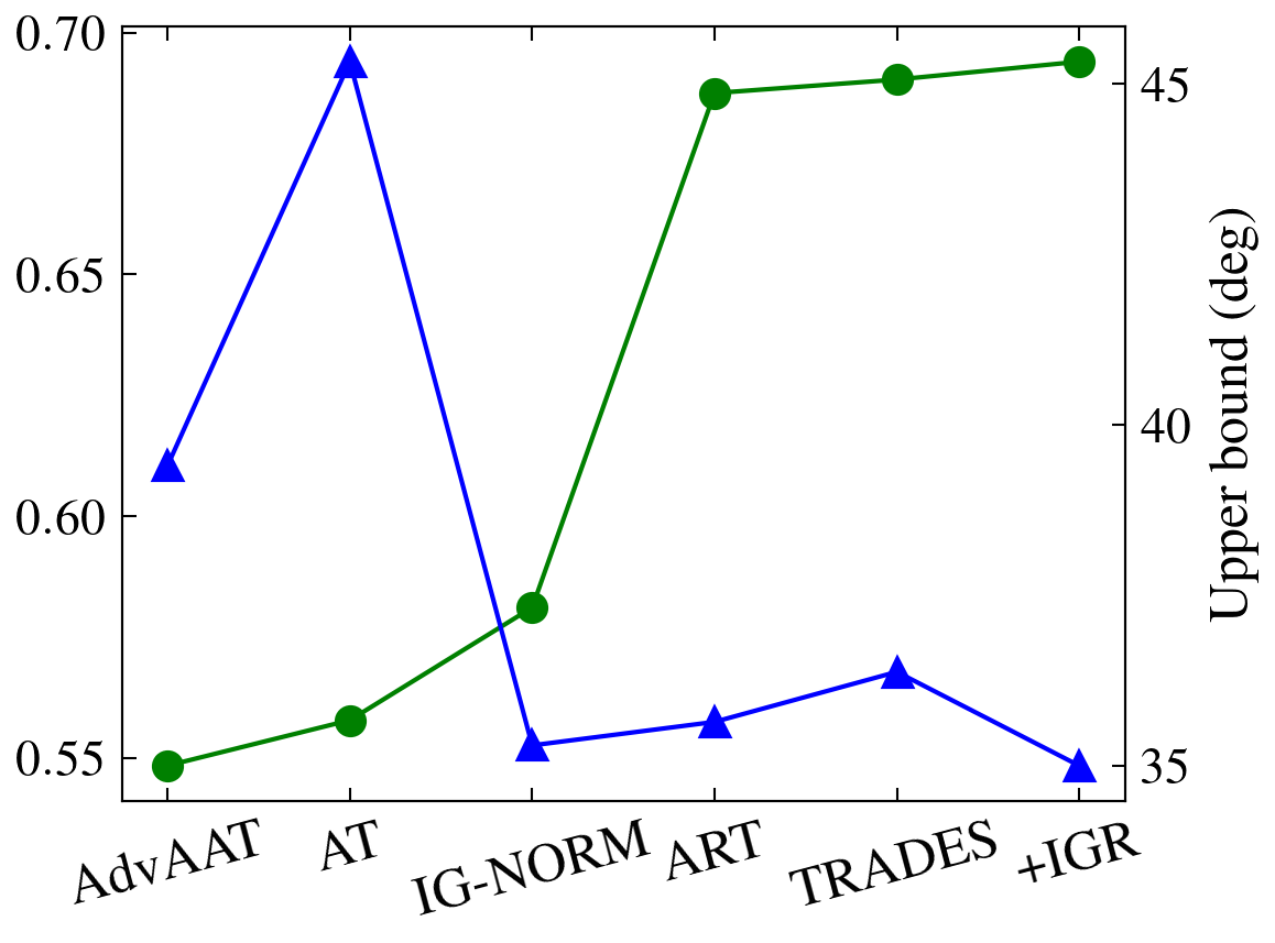
(c) CIFAR-10

Figure 2: Comparison between Kendall’s rank correlation and the theoretical bound of cosine distance. For clear comparison, we convert the cosine distance to angles in degrees.

5.3 Evaluation of upper bounds under $\ell_{\infty}$-norm constraint and label constraint

Table 4: Evaluation of upper bounds $\ell_{\infty}$-norm constraint and label constraint.

Model	Kendall	$\widehat{T}_{e}$	$T_{e}$	$\widehat{T}_{c}$($\deg$)	$T_{c}$($\deg$)
$\varepsilon=0.05$	MNIST
AT	0.1846	0.3461	0.7752	15.3616	38.7024
IG-NORM	0.1562	0.6836	1.2046	16.4506	31.8791
AdvAAT	0.3791	1.6269	2.1992	11.3173	26.3000
ART	0.1439	1.4193	2.8218	12.8025	64.3115
TRADES	0.2127	1.1779	2.2216	15.9881	33.4681
TRADES+IGR	0.4537	1.2991	2.0386	17.5923	26.5748
$\varepsilon=0.05$	Fashion-MNIST
AT	0.1516	0.0990	0.2802	18.9720	55.1501
IG-NORM	0.3446	0.2384	0.8819	12.6023	46.4270
AdvAAT	0.5810	0.1938	0.9206	9.4499	44.9184
ART	0.2079	0.1660	0.7215	9.6582	53.7281
TRADES	0.2582	0.1042	0.4536	13.7010	51.6448
TRADES+IGR	0.6565	0.0722	0.2526	15.0947	44.4703
$\varepsilon=0.1$	CIFAR-10
AT	0.5578	0.4058	0.7649	26.6195	45.3223
IG-NORM	0.5811	0.1997	0.4783	21.6311	35.2981
AdvAAT	0.5484	0.2293	0.5211	28.7342	39.3981
ART	0.6875	0.3128	0.6734	31.0090	35.6422
TRADES	0.6903	0.2322	0.5001	22.9779	36.3759
TRADES+IGR	0.6940	0.2474	0.5236	23.2356	35.0009

Table 5: Evaluation of tightness of the bounds in Euclidean distance for $\ell_{2}$ and $\ell_{\infty}$ cases.

	MNIST			Fashion-MNIST			CIFAR-10
$\ell_{2}(\varepsilon=)$	0.05	0.1	0.2	0.05	0.1	0.2	0.1	0.2	0.3
AT	0.0260	0.0320	0.0140	0.0078	0.0130	0.1207	0.0004	0.0045	0.0134
IG-NORM	0.0391	0.0597	0.0291	0.0121	0.0171	0.0742	0.0016	0.0210	0.0448
AdvAAT	0.0290	0.0465	0.0294	0.0103	0.0167	0.0183	0.0037	0.0090	0.0181
ART	0.0178	0.0115	0.0182	0.0029	0.0239	0.0011	0.0019	0.0031	0.0141
TRADES	0.0014	0.0032	0.0104	0.0037	0.0082	0.0723	0.0028	0.0048	0.0147
TRADES+IGR	0.0010	0.0038	0.0041	0.0064	0.0134	0.0385	0.0016	0.0100	0.0126
$\ell_{\infty}(\varepsilon=)$	0.01	0.03	0.05	0.01	0.03	0.05	4/255	8/255	0.1
AT	0.0021	0.0035	0.0117	0.0004	0.0352	0.0708	0.0025	0.0053	0.1381
IG-NORM	0.0001	0.0062	0.0105	0.0010	0.0590	0.1069	0.0026	0.0145	0.0003
AdvAAT	0.0004	0.0223	0.0901	0.0136	0.0847	0.1665	0.0448	0.1513	0.2078
ART	0.0082	0.0112	0.0233	0.0424	0.1049	0.1467	0.0118	0.0412	0.0870
TRADES	0.0001	0.0046	0.0026	0.0014	0.0337	0.0634	0.0068	0.0043	0.0530
TRADES+IGR	0.0016	0.0143	0.1389	0.0014	0.0375	0.0682	0.0016	0.0090	0.0197

In this subsection, the upper bounds of attribution deviations under $\ell_{\infty}$ attacks are presented. Instead of the much looser bound derived from $\ell_{p}$-norm relaxation (Corollary 1), the upper bound is computed from $T_{e}=\varepsilon\sqrt{\sum|P_{ij}|}$ as introduced in Sec. 4.3 and 4.4 . Moreover, the empirical attribution robustness is also provided using Kendall’s rank correlation [14] for comparison of theoretical and empirical protection. It should be emphasized that all the previous attribution robustness studies are based on $\ell_{\infty}$-norm constraints. Kendall’s rank correlation, which is non-differentiable, is used as one of the indexes to measure the difference between the original attributions and the attributions attacked by IFIA under $\ell_{\infty}$-norm constraints. From the results in Table 4, we see that the computed theoretical upper bounds are valid to measure the worst-case attribution deviations. For each dataset and each model, the sample mean of attribution distances is strictly smaller than the theoretical distance. Because of the relaxation, all attacked attributions are bounded by $T_{e}$. There is no outlier, and there is no need to use the generalized bound $T^{\prime}_{e}$. Moreover, the results also show that for a model with a larger Kendall’s rank correlation, the theoretical cosine distance upper bound is more likely to be smaller (see Fig. 2), which means that the model is more difficult to be attacked. This also confirms that cosine similarity is positively correlated to Kendall’s rank correlation as proposed in Wang & Kong [32].

5.4 Evaluation of the tightness of bounds

In addition, we further report the minimum Euclidean gaps between samples and theoretical bounds in Table 5 to measure the tightness of the provided bounds, which is defined as

$$r=\min_{0\leq i\leq n}T^{(i)}_{e}-\widehat{T}_{e}^{(i)}$$ (12)

Note that the superscript $(i)$ represents the $i$-th sample and $T^{(i)}_{e}$ is replaced by $T^{\prime(i)}_{e}$ in $\ell_{2}$-norm cases. $r$ is a straightforward measurement of the theoretical bound. We notice that although the mean of theoretical bounds sometimes are multiple times larger than the sample mean distance, the tightest bound can be only $10^{-4}$ greater than the sample distance. We also observe that the values of $r$ are all positive, which also indicates that there is no perturbed attribution that violates our theoretical bounds.

We also provide the visualizations of the distribution of the gap between theoretical bounds and attribution differences from real data in Appendix D. The values are directly computed using $T^{(i)}_{e}-\widehat{T}_{e}^{(i)}$. As we can observe from the figures, all values are positive, which verifies the validity of our bounds, and most of the values are lying close to $0$, which shows the tightness of the bounds.

6 Conclusion

In this paper, an upper bound that measures the worst-case attribution deviations is proposed. The bound is formulated as the optimum value of a constrained optimization problem. The optimization problem is constrained on the size of perturbation and the unchanged classification label after being perturbed. For each of the two metrics of the attribution difference, Euclidean and cosine distances, the problem is solved based on the first-order Taylor series and the estimation of attribution gradients and the solution bounds the attribution deviations under both $\ell_{2}$ and $\ell_{\infty}$-norm attacks. Experimental results validate the effectiveness of the proposed bounds.

Appendix A Proofs

A.1 Proof of Corollary 1

Before we prove Corollary 1, We first introduce the following lemma.

Lemma 1.

For $0<q<p$, the following inequality holds:

$$\|{\bm{x}}\|_{q}\leq d^{\frac{1}{q}-\frac{1}{p}}\|{\bm{x}}\|_{p}$$ (13)

where ${\bm{x}}\in\mathbb{R}^{d}$.

Proof.

Consider $\bm{u},\bm{v}\in\mathbb{R}^{d}$, using the Hölder’s Inequality that for $m,n$ satisfying $\frac{1}{m}+\frac{1}{n}=1$,

$$\sum_{i}|u_{i}||v_{i}|\leq\left(\sum_{i}|u_{i}|^{m}\right)^{\frac{1}{m}}\left(\sum_{i}|v_{i}|^{n}\right)^{\frac{1}{n}}.$$ (14)

If we take $|u_{i}|=|x_{i}|^{q}$, $v_{i}=1$, $m=\frac{p}{q}$ and $n=\frac{p}{p-q}$, we get

$$\sum_{i}|x_{i}|^{q}\leq\left(\sum_{i}|x_{i}|^{p}\right)^{\frac{q}{p}}d^{\frac{p-q}{p}}$$ (15)

By taking the power of $\frac{1}{q}$ on both sides, we have

$$\left(\sum_{i}|x_{i}|^{q}\right)^{\frac{1}{q}}\leq\left(\sum_{i}|x_{i}|^{p}\right)^{\frac{1}{p}}d^{\frac{1}{q}-\frac{1}{p}}$$ (16)

which concludes the proof. ∎

See 1

Proof.

Using Lemma 1, we have $\|\bm{\delta}\|_{2}\leq d^{\frac{1}{2}-\frac{1}{p}}\|\bm{\delta}\|_{p}$. Similar to the proof of Theorem 1,

$$\|g^{y}({\bm{x}}+\bm{\delta})-g^{y}({\bm{x}})\|_{2}^{2}\leq\lambda_{max}\|\bm{\delta}\|_{2}^{2}\leq\lambda_{max}\left(d^{\frac{1}{2}-\frac{1}{p}}\|\bm{\delta}\|_{p}\right)^{2}\leq\lambda_{max}\left(d^{\frac{1}{2}-\frac{1}{p}}\varepsilon\right)^{2}$$ (17)

Therefore,

$$\|g^{y}({\bm{x}}+\bm{\delta})-g^{y}({\bm{x}})\|_{2}\leq d^{\frac{1}{2}-\frac{1}{p}}\xi_{max}\varepsilon$$ (18)

∎

A.2 Proof of Theorem 2

See 2

Proof.

Recall that under the local linearity assumption,

$$\|g^{y}({\bm{x}}+\bm{\delta})-g^{y}({\bm{x}})\|_{2}^{2}\leq\bm{\delta}^{\top}P\bm{\delta}=\sum_{i,j}P_{ij}\delta_{i}\delta_{j}.$$ (19)

Since $P_{ij}\leq|P_{ij}|$ and $\delta_{i}\delta_{j}\leq\|\bm{\delta}\|^{2}_{\infty}\leq\varepsilon^{2}$ for all $i,j$, we can easily prove the theorem that

$$\|g^{y}({\bm{x}}+\bm{\delta})-g^{y}({\bm{x}})\|_{2}^{2}\leq\varepsilon^{2}\sum_{i,j}|P_{ij}|.$$ (20)

∎

A.3 Proof of Proposition 1

See 1

Proof.

Recall that we denote the gradient-based attribution satisfying the completeness axiom of ${\bm{x}}$ on target label $y$ by $g^{y}({\bm{x}})$, e.g., integrated gradients. Similarly, we denote the attribution on a different label $y^{\prime}$ by $g^{y^{\prime}}({\bm{x}})$. Given the perturbation $\bm{\delta}$, according to the above assumption, we can write that

$$g^{y}({\bm{x}}+\bm{\delta})=g^{y}({\bm{x}})+\nabla g^{y}({\bm{x}})^{\top}\bm{\delta}$$ (21)

Similarly, the approximation of $g^{y^{\prime}}({\bm{x}}+\bm{\delta})$ is given by:

$$g^{y^{\prime}}({\bm{x}}+\bm{\delta})=g^{y^{\prime}}({\bm{x}})+\nabla g^{y^{\prime}}({\bm{x}})^{\top}\bm{\delta}$$ (22)

According to the completeness axiom, given an all one vector $\Delta=(1,\ldots,1)^{\top}$, we have

$$\Delta^{\top}g^{y}({\bm{x}})=f_{y}({\bm{x}}).$$ (23)

Consider the perturbation $\bm{\delta}$, if $\bm{\delta}$ does not change the label of ${\bm{x}}$ from $y$ to $y^{\prime}$, then $f_{y^{\prime}}({\bm{x}}+\bm{\delta})<f_{y}({\bm{x}}+\bm{\delta})$, i.e.,

$$\Delta^{\top}g^{y^{\prime}}({\bm{x}}+\bm{\delta})<\Delta^{\top}g^{y}({\bm{x}}+\bm{\delta}),$$ (24)

which gives

$$\Delta^{\top}g^{y^{\prime}}({\bm{x}})+\Delta^{\top}\nabla g^{y^{\prime}}({\bm{x}})^{\top}\bm{\delta}<\Delta^{\top}g^{y}({\bm{x}})+\Delta^{\top}\nabla g^{y}({\bm{x}})^{\top}\bm{\delta}.$$ (25)

By rearranging the above inequality, we have

$$\left(\left(\nabla g^{y^{\prime}}({\bm{x}})-\nabla g^{y}({\bm{x}})\right)\Delta\right)^{\top}\bm{\delta}<f_{y}({\bm{x}})-f_{y^{\prime}}({\bm{x}}).$$ (26)

∎

A.4 Proof of Corollary 2

See 2

Proof.

The corollary can be proved using the geometric property (see Fig. 1(a)) that

$$\sin(g^{y}({\bm{x}}+\bm{\delta}),g^{y}({\bm{x}}))\leq\frac{T(\varepsilon;{\bm{x}})}{\|g^{y}({\bm{x}})\|_{2}},$$ (27)

and,

$$\text{cosd}(g^{y}({\bm{x}}+\bm{\delta}),g^{y}({\bm{x}})) =1-\cos(g^{y}({\bm{x}}+\bm{\delta}),g^{y}({\bm{x}}))$$ (28)

$$=1-\sqrt{1-\sin^{2}(g^{y}({\bm{x}}+\bm{\delta}),g^{y}({\bm{x}}))}$$ (29)

$$\leq 1-\sqrt{1-\frac{T(\varepsilon;{\bm{x}})^{2}}{\|g^{y}({\bm{x}})\|_{2}^{2}}}$$ (30)

∎

Appendix B Analysis of local linearity assumption

B.1 Evaluation of local linearity assumption of attribution functions

The theories of this work are based on the local linearity assumption that $g^{y}({\bm{x}})$ is linear within $\mathcal{B}_{\varepsilon}({\bm{x}})=\{{\bm{x}}+\bm{\delta}|\|\bm{\delta}\|_{p}\leq\varepsilon\}$. It is worth noting that such local linearity is a valid assumption for smooth functions, which can be achieved by both adversarial and attributional robust methods. Adversarial defense methods look for locally linearity functions to reduce the impact of adversarial attacks [22, 35]. Similarly, attributional defense methods train for smooth gradients to defend against attribution attacks [33]. It is also a common practice in related literature [7, 11, 27, 16, 38] to make similar assumptions.

Furthermore, the validity of this assumption also depends on the size of $\bm{\delta}$. The perturbation $\bm{\delta}$ is restricted within a small $\ell_{p}$ ball around ${\bm{x}}$ to ensure that the perturbed images are visually indistinguishable comparing to its original counterpart. The maximum allowable size $\varepsilon$ for $\bm{\delta}$ is relatively small compared with the intensity range of the original image. When $\bm{\delta}$ is small, the remainder of the Taylor series of $g^{y}({\bm{x}})$ is negligible and the local linearity assumption is valid. As shown in Figure 3, the value of $\eta({\bm{x}},\bm{\delta})=\|g^{y}({\bm{x}})-g^{y}({\bm{x}}+\bm{\delta})-\bm{\delta}^{\top}\nabla g^{y}({\bm{x}})\|_{2}$ is small and negligible when $\|\bm{\delta}\|_{\infty}$ is small.

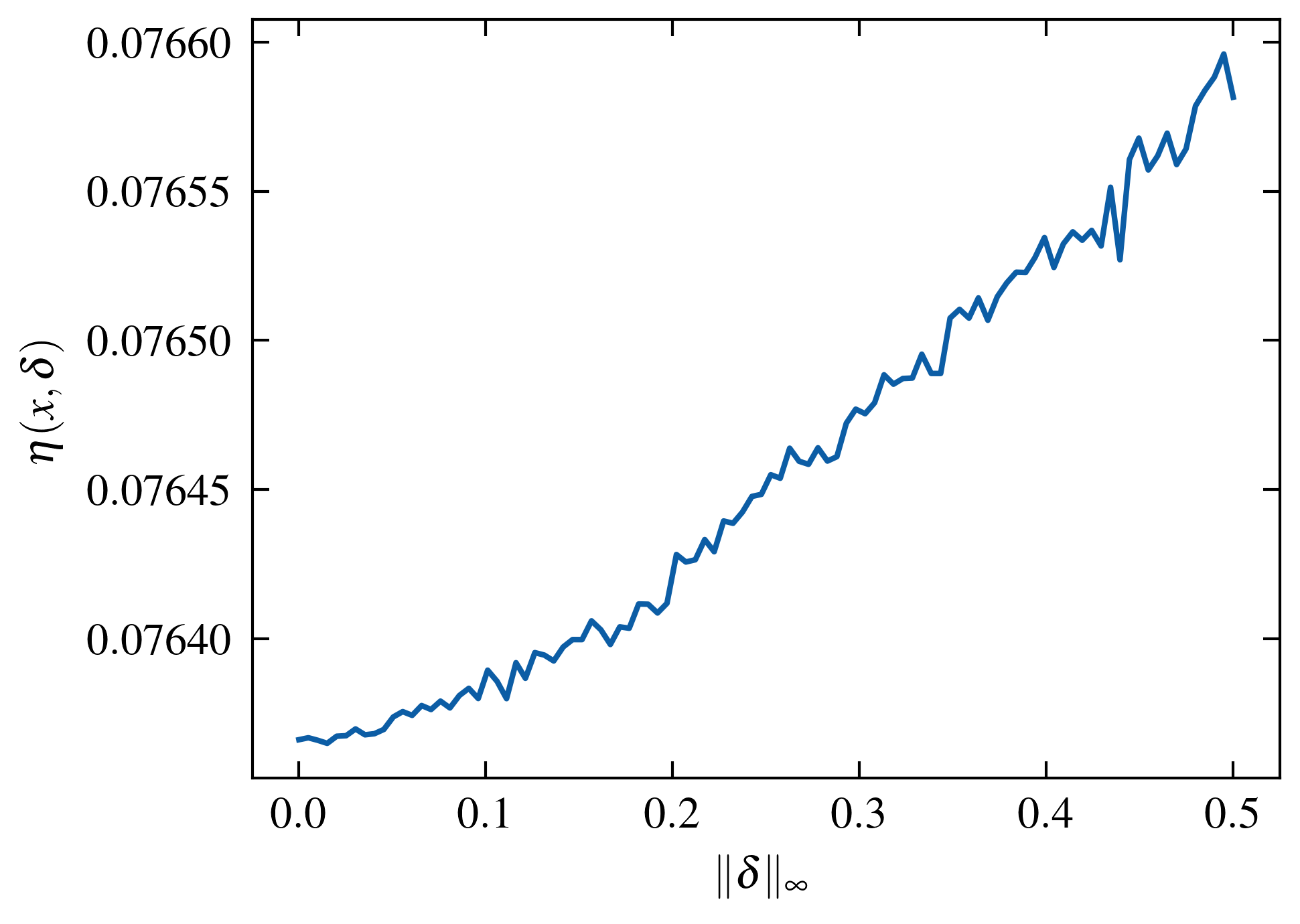
(a) AT

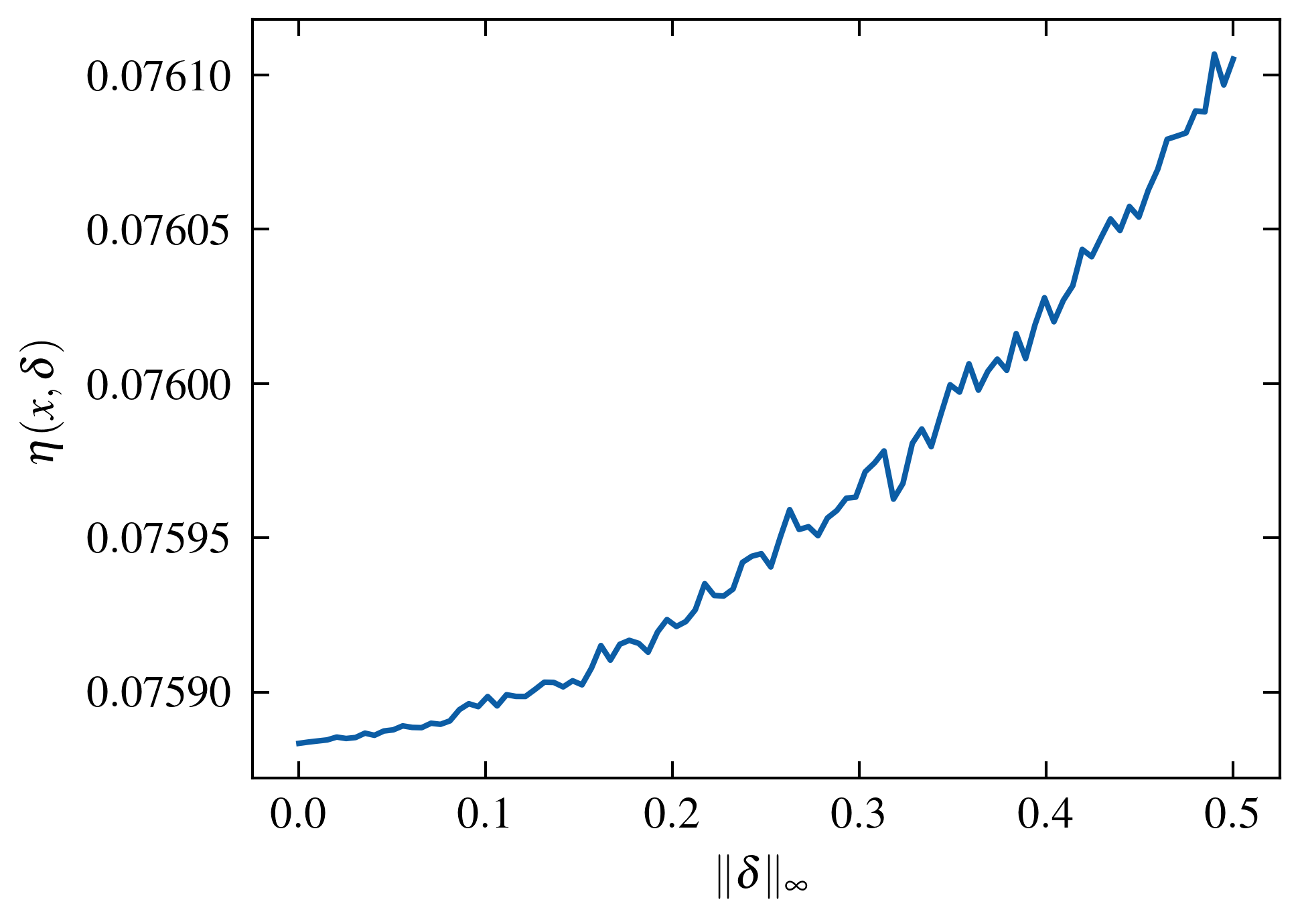
(b) IG-NORM

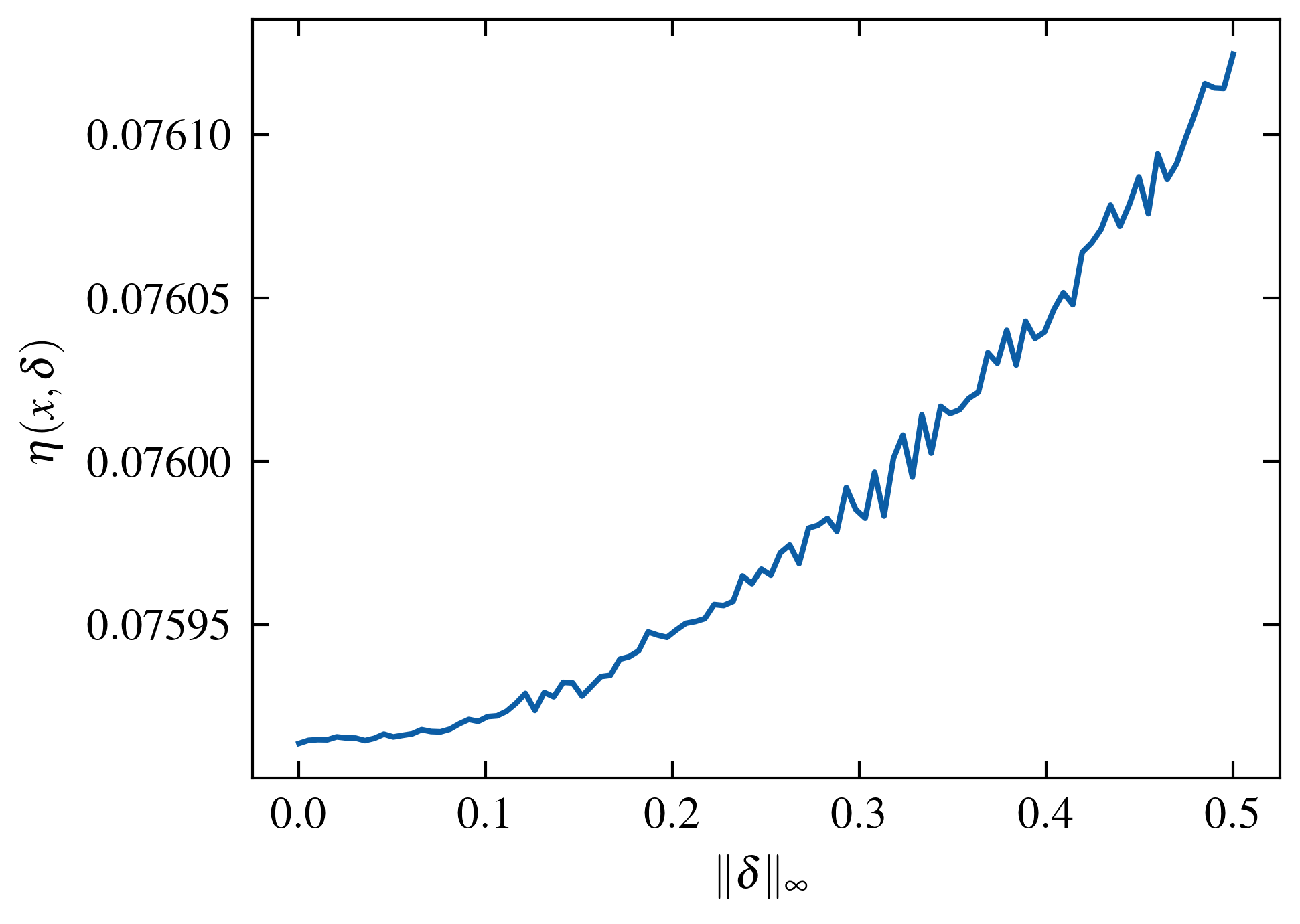
(c) AdvAAT

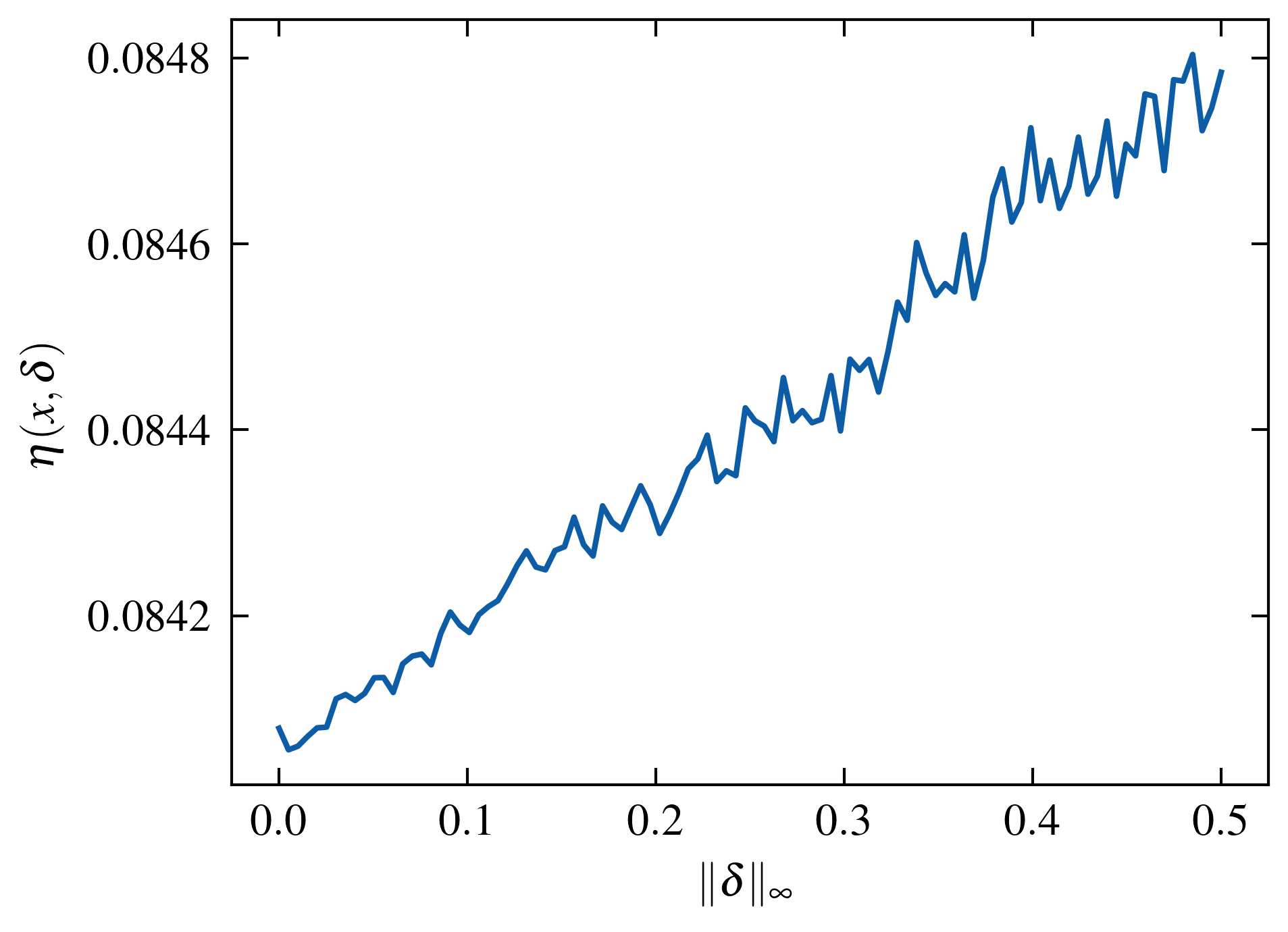
(d) ART

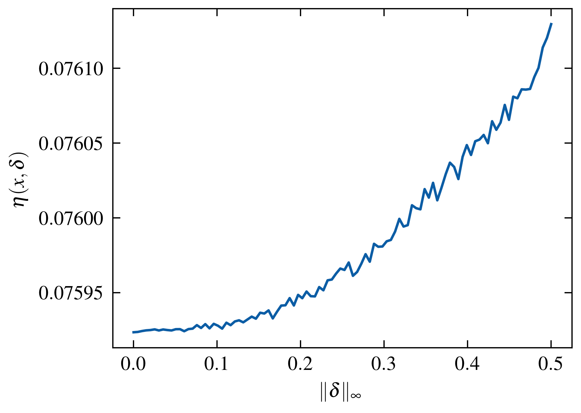
(e) TRADES

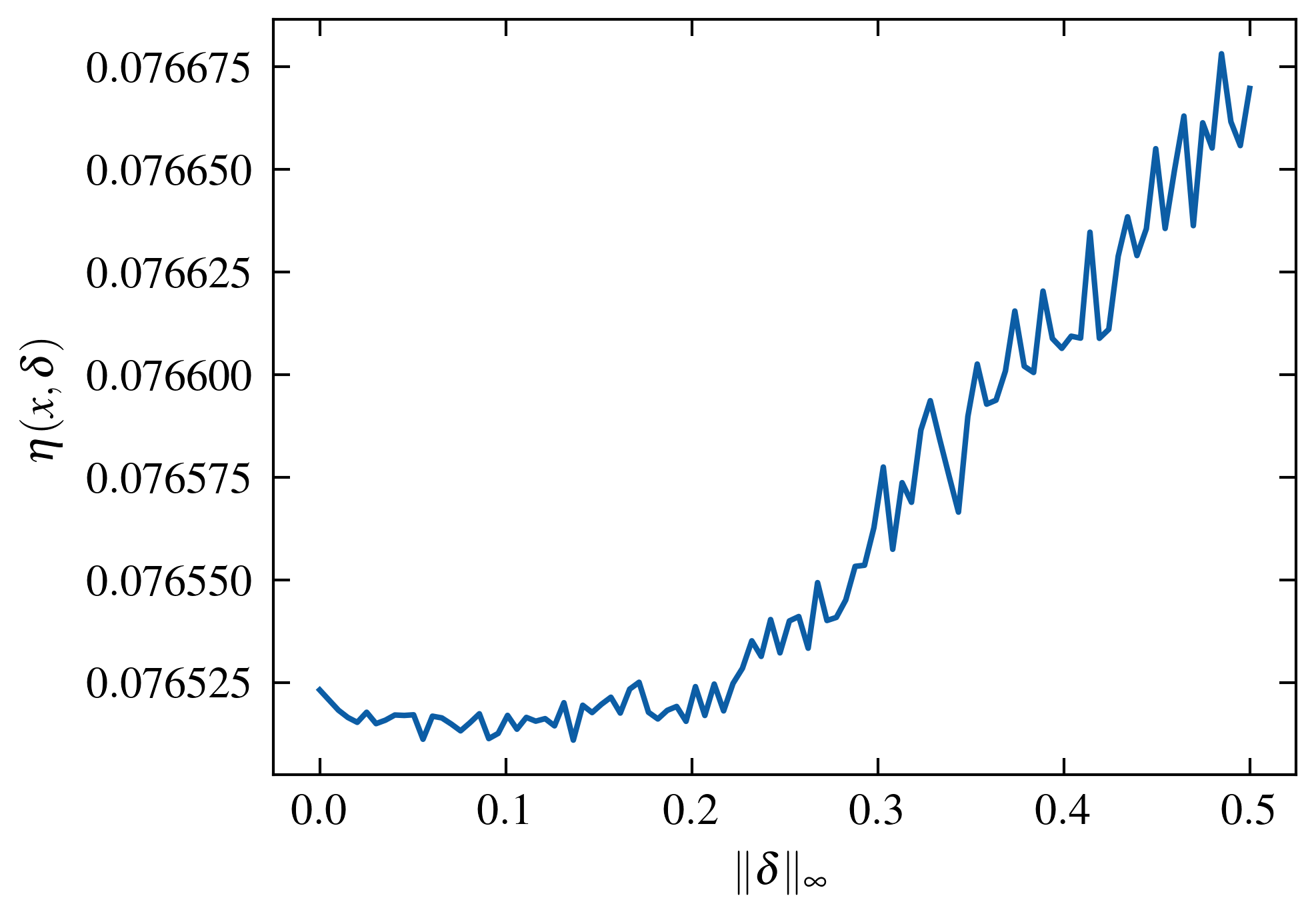
(f) TRADES+IGR

Figure 3: Values of $\eta$ for different $\|\bm{\delta}\|_{\infty}$ computed from CIFAR-10 using integrated gradients. The magnitudes are ranging from $0.07$ to $0.09$ and are negligible comparing with the average norm of attributions which is $3.47$ on CIFAR-10.

B.2 Generalization of Theorem 1

Theorem 3.

Given a twice-differentiable classifier $f:\mathbb{R}^{d}\rightarrow\mathbb{R}^{k}$, and its attribution $g^{y}$ on label $y$, denote the Taylor series of $g^{y}({\bm{x}}+\bm{\delta})$ as $g^{y}({\bm{x}})+\bm{\delta}^{\top}\nabla g^{y}({\bm{x}})+R_{1}({\bm{x}})$. If $-(c-1)\bm{\delta}^{\top}\nabla g^{y}({\bm{x}})\preceq R_{1}({\bm{x}})\preceq(c-1)\bm{\delta}^{\top}\nabla g^{y}({\bm{x}})$ for a constant $c\geq 1$, where $\preceq$ refers to element-wise less than or equal to, then for all perturbations $\|\bm{\delta}\|_{2}\leq\varepsilon$,

$$\|g^{y}({\bm{x}}+\bm{\delta})-g^{y}({\bm{x}})\|_{2}\leq c\xi_{max}\varepsilon,$$

where $\xi_{max}$ is the largest singular value of $H=\nabla g^{y}({\bm{x}})$.

Proof.

Based on the Taylor series of $g^{y}({\bm{x}})$ and the above condition, we have

$$\|g^{y}({\bm{x}}+\bm{\delta})-g^{y}({\bm{x}})\|_{2}^{2}\leq\|\bm{\delta}^{\top}\nabla g^{y}({\bm{x}})+(c-1)\bm{\delta}^{\top}\nabla g^{y}({\bm{x}})\|_{2}^{2} =c^{2}\bm{\delta}^{\top}\nabla g^{y}({\bm{x}})\nabla g^{y}({\bm{x}})^{\top}\bm{\delta}$$ (31)

$$=c^{2}\frac{\bm{\delta}^{\top}}{\|\bm{\delta}\|_{2}}P\frac{\bm{\delta}}{\|\bm{\delta}\|_{2}}\cdot\|\bm{\delta}\|^{2}_{2}$$ (32)

$$\leq c^{2}\lambda_{max}\|\bm{\delta}\|^{2}_{2}\leq c^{2}\lambda_{max}\varepsilon^{2}$$ (33)

where $\lambda_{max}$ is the largest eigenvalue of $P=HH^{\top}=\nabla g^{y}({\bm{x}})\nabla g^{y}({\bm{x}})^{\top}$, and $\bm{v}_{max}$ is the corresponding eigenvector. The equality in Eq. 33 is achieved when $\bm{\delta}$ is $\varepsilon\bm{v}_{max}$ or $-\varepsilon\bm{v}_{max}$. Since the singular values of $H$ are equal to the square root of the eigenvalues of $P$, then,

$$\|g^{y}({\bm{x}}+\bm{\delta})-g^{y}({\bm{x}})\|_{2}\leq c\sqrt{\lambda_{max}}\varepsilon=c\xi_{max}\varepsilon.$$ (34)

∎

This is a generalized version of Theorem 1 that is applicable for all twice-differentiable classifiers. Under local linearity assumption, $R_{1}({\bm{x}})=0$, which means $c=1$, the result coincides with the original version of Theorem 1.

B.3 Derivation of Eq. (11)

By Taylor expansion, $g^{y}({\bm{x}}+\bm{\delta})-g^{y}({\bm{x}})=\bm{\delta}^{\top}\nabla g^{y}({\bm{x}})+R_{1}({\bm{x}})$, where $R_{1}$ is the first order Taylor remainder. Thus, we have

$$\|R_{1}({\bm{x}})\|_{2}\geq\|g^{y}({\bm{x}}+\bm{\delta})-g^{y}({\bm{x}})\|_{2}-\|\bm{\delta}^{\top}\nabla g^{y}({\bm{x}})\|_{2}$$ (35)

Take $c=\frac{\|R_{1}({\bm{x}})\|_{2}}{\|\bm{\delta}^{\top}\nabla g^{y}({\bm{x}})\|_{2}}+1$,

$$\|\bm{\delta}^{\top}\nabla g^{y}({\bm{x}})\|_{2}+\|R_{1}({\bm{x}})\|_{2}=c\|\bm{\delta}^{\top}\nabla g^{y}({\bm{x}})\|_{2},$$ (36)

and it would be the worst-case for the linear assumption when $\bm{\delta}=\varepsilon\bm{v}_{max}$. By taking $\varepsilon\bm{v}_{max}$ as $\bm{\delta}$, $\|R_{1}({\bm{x}})\|_{2}$ can be estimated by

$$\max\left\{0,\|g^{y}({\bm{x}}+\varepsilon\bm{v}_{max})-g^{y}({\bm{x}})\|_{2}-\|\varepsilon\bm{v}_{max}^{\top}\nabla g^{y}({\bm{x}})\|_{2}\right\}.$$ (37)

Since $\|g^{y}({\bm{x}}+\varepsilon\bm{v}_{max})-g^{y}({\bm{x}})\|_{2}-\|\varepsilon\bm{v}_{max}^{\top}\nabla g^{y}({\bm{x}})\|_{2}\leq\|R_{1}({\bm{x}})\|_{2}$. Putting Eq. (37) into $c$ and using the result in Eq. (6), we have

$$c =\max\left\{0,\frac{\|g^{y}({\bm{x}}+\varepsilon\bm{v}_{max})-g^{y}({\bm{x}})\|_{2}-\|\varepsilon\bm{v}_{max}^{\top}\nabla g^{y}({\bm{x}})\|_{2}}{\xi_{max}\varepsilon}\right\}+1$$ (38)

$$=\max\left\{1,\frac{\|g^{y}({\bm{x}}+\varepsilon\bm{v}_{max})-g^{y}({\bm{x}})\|_{2}}{\xi_{max}\varepsilon}\right\}.$$ (39)

Appendix C Analysis of attribution gradients

C.1 The gradient of integrated gradients

We provide the justification showing that the gradient of IG is diagonal-dominated. Consider that

$$\text{IG}({\bm{x}})_{i}=x_{i}\times\frac{1}{m}\sum_{\alpha=1}^{m}\frac{\partial f(\frac{\alpha}{m}{\bm{x}})}{\partial x_{i}}$$ (40)

and

$$\nabla\text{IG}({\bm{x}})_{ij}=\frac{\partial\text{IG}({\bm{x}})_{i}}{\partial x_{j}}$$ (41)

If $i\neq j$, then

$$\frac{\partial\text{IG}({\bm{x}})_{i}}{\partial x_{j}}=x_{i}\cdot\frac{1}{m}\sum_{\alpha=1}^{m}\frac{\partial^{2}f(\frac{\alpha}{m}{\bm{x}})}{\partial x_{i}\partial x_{j}}\times\frac{\alpha}{m}$$ (42)

If $i=j$, then

$$\frac{\partial\text{IG}({\bm{x}})_{i}}{\partial x_{j}}=\frac{1}{m}\sum_{\alpha=1}^{m}\frac{\partial f(\frac{\alpha}{m}{\bm{x}})}{\partial x_{j}}+x_{i}\cdot\frac{1}{m}\sum_{\alpha=1}^{m}\frac{\partial^{2}f(\frac{\alpha}{m}{\bm{x}})}{\partial x_{i}\partial x_{j}}\times\frac{\alpha}{m}$$ (43)

Denote that $H^{(\alpha)}_{ij}=\frac{\partial^{2}f(\frac{\alpha}{m}{\bm{x}})}{\partial x_{i}\partial x_{j}}$, i.e., $H^{(\alpha)}$ is the Hessian matrix of $f(\frac{\alpha}{m}{\bm{x}})$. Thus

$$\frac{\partial\text{IG}({\bm{x}})_{i}}{\partial x_{j}}=\begin{cases}\frac{1}{m}\sum_{\alpha=1}^{m}\nabla f(\frac{\alpha}{m}{\bm{x}})+x_{i}\cdot\frac{\alpha}{m^{2}}H^{(\alpha)}_{ij},\quad i=j\\ x_{i}\cdot\sum_{\alpha=1}^{m}\frac{\alpha}{m^{2}}H^{(\alpha)}_{ij},\quad i\neq j\end{cases}$$ (44)

In matrix form,

$$\nabla\text{IG}=\text{diag}\left(\frac{1}{m}\sum_{\alpha=1}^{m}\nabla f(\frac{\alpha}{m}{\bm{x}})\right)+[{\bm{x}},\cdots,{\bm{x}}]\otimes\frac{\alpha}{m^{2}}\sum_{\alpha=1}^{m}H^{(\alpha)}$$ (45)

If we use softplus as an activation function, i.e., $g({\bm{x}})=\frac{1}{\beta}\log(1+\exp(\beta{\bm{x}}))$, then,

$$g^{\prime\prime}({\bm{x}})=\frac{\beta e^{\beta{\bm{x}}}}{(e^{\beta{\bm{x}}}+1)^{2}}$$ (46)

and

$$\lim_{\beta\rightarrow\infty}g^{\prime\prime}({\bm{x}})=0$$ (47)

As $\beta\rightarrow\infty$, $H^{(\alpha)}$ will tend to $0$, and the second term in Eq. 45 will tend to 0. At the same time, if we choose the number of steps in IG, $m$ larger, $\frac{\alpha}{m^{2}}$ will converge to $0$ faster than $\frac{1}{m}$. Therefore, $\nabla\text{IG}$ will be diagonal-dominated.

C.2 Additional visualization of attribution gradients

We provide the first 100-dimensions heatmaps of absolute values of attribution gradients, i.e., gradients of IG, on MNIST and Fashion-MNIST in addition to CIFAR-10 presented in Fig. 1(b). Moreover, the complete heatmaps for all the three datasets are also presented. As observed in Figs. 4, 5, 6 and 7, the matrices of attribution gradients are diagonal-dominant.

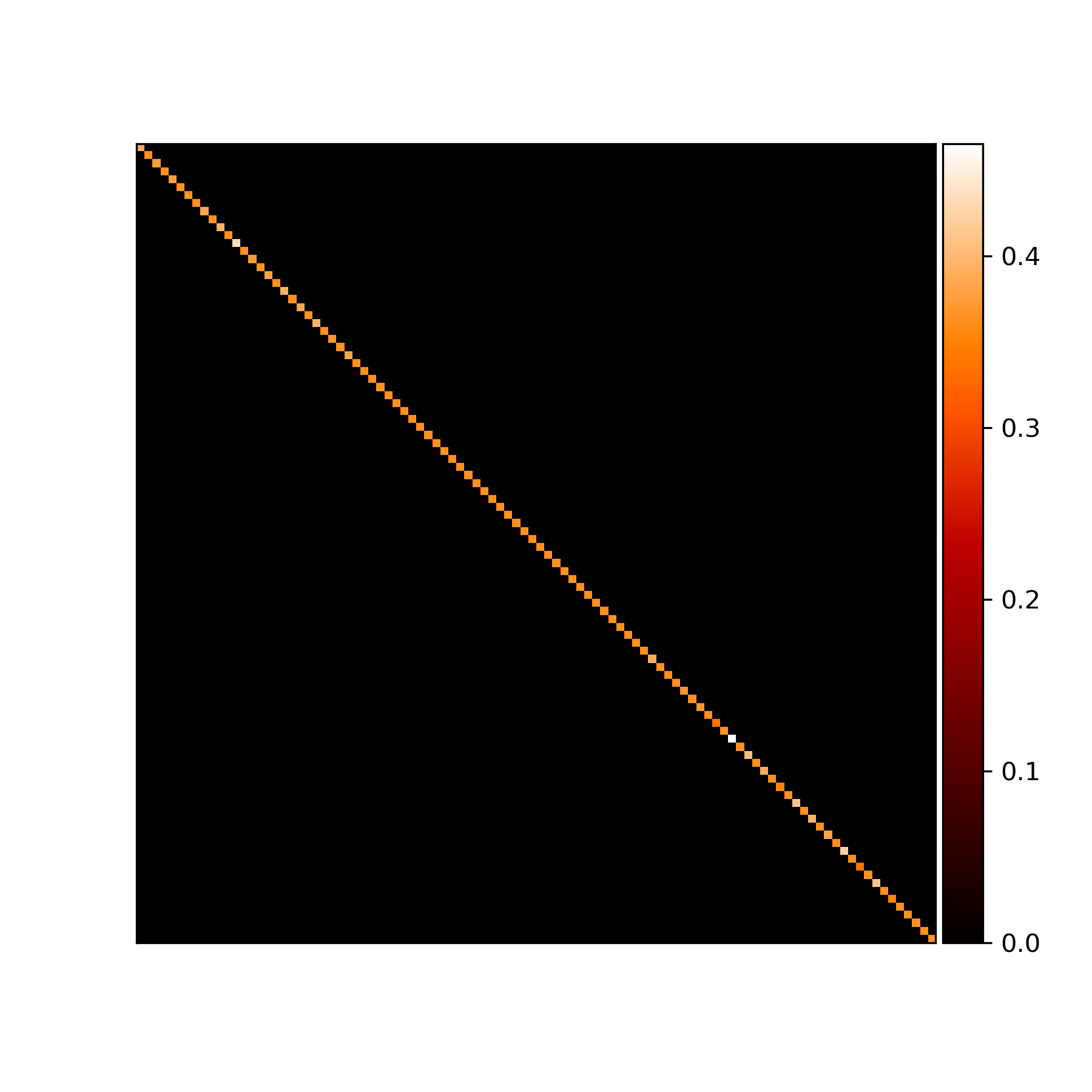
(a)

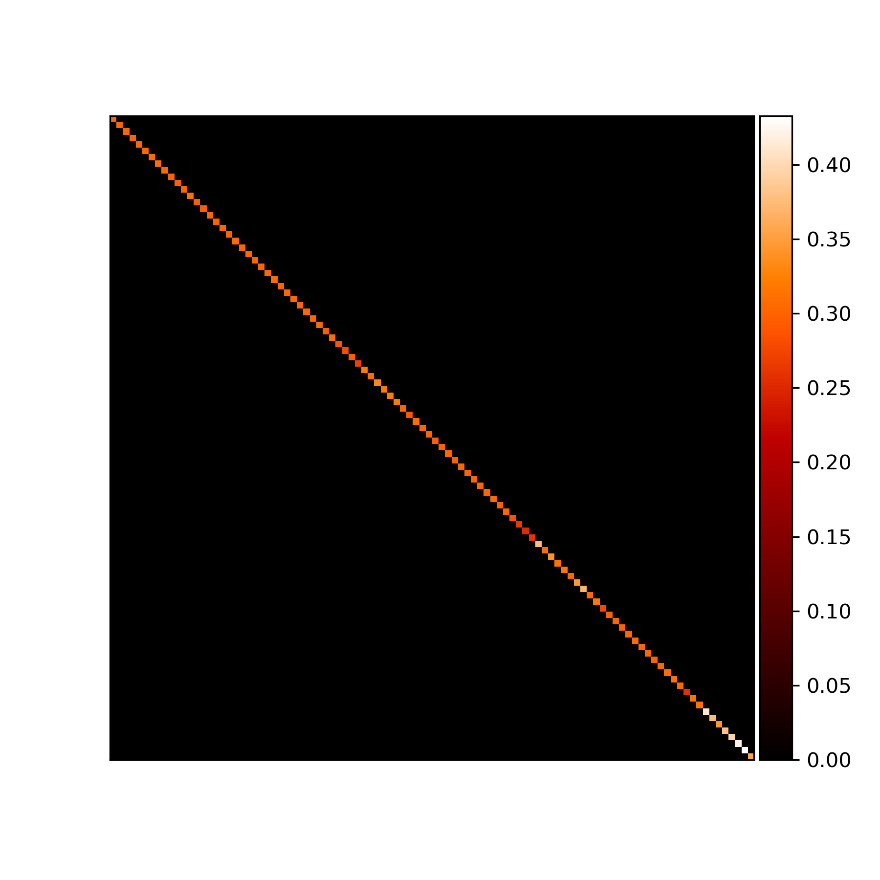
(b)

Figure 4: The first 100 dimensions of gradient attribution generated from (a) MNIST and (b) Fashion-MNIST.

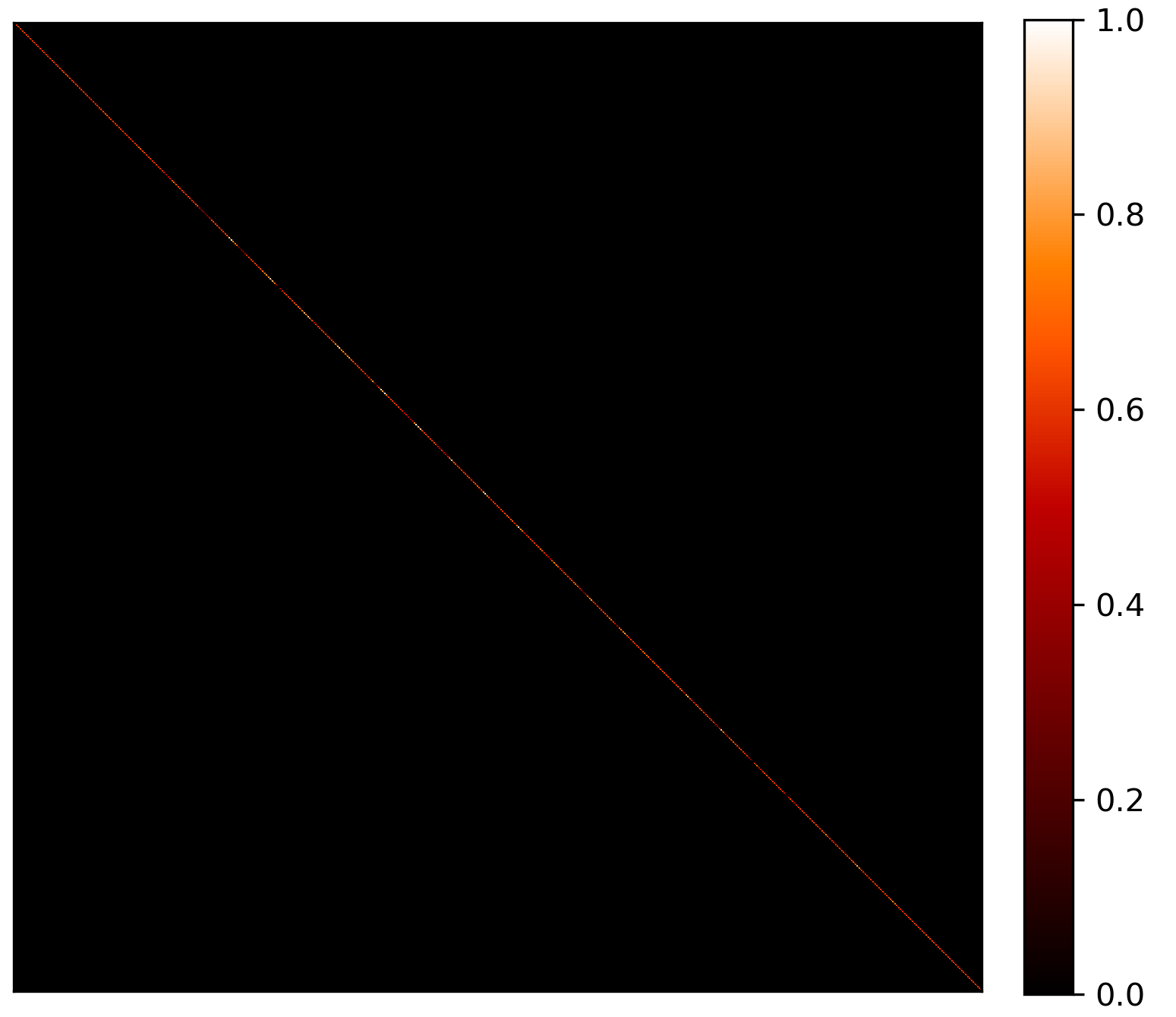
Figure 5: The full heatmap of attribution gradients of MNIST in size $784\times 784$.

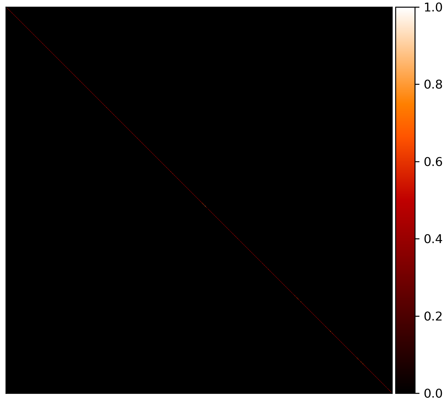
Figure 6: The full heatmap of attribution gradients of Fashion-MNIST in size $784\times 784$.

Figure 7: The full heatmap of attribution gradients of CIFAR-100 in size $3072\times 3072$.

Appendix D Additional experimental results

D.1 Additional results of upper bound on more models without the label constraint

In this subsection, we evaluate the proposed upper bound without the label constraint for the other models, apart from TRADES+IGR in the paper. The perturbation size is chosen to be $0.1$ for all evaluations. As in Sec. 5, we use Theorem 1 and 2 to compute $T_{e}=\xi_{max}\varepsilon$ and extend it to $T_{c}$ using Eq. 10. The modified upper bound $T^{\prime}_{e}=c\xi_{max}\varepsilon$ is also provided to address the inaccurate Taylor approximation (less than $1\%$). $\widehat{T}_{e}$ and $\widehat{T}_{c}$ are computed from the corresponding average attribution differences. The results are given in Table 6. It is shown that the sample distances under both Euclidean and cosine metrics are bounded by $T^{\prime}_{e}$ and $T_{c}$ as expected. All the distortion caused by the attacks i.e., $\widehat{T}_{e}$ and $\widehat{T}_{c}$ are smaller than $T^{\prime}_{e}$ and $T_{c}$.

Table 6: Evaluation of upper bounds without the label constraint. The cosine distance values $\widehat{T}_{c}$ and $\widehat{T}^{\prime}_{c}$ are converted to degrees for easier comparison.

	SM					Input*gradient					IG
$\ell_{2}$	$\widehat{T}_{e}$	$T_{e}$	$T^{\prime}_{e}$	$\widehat{T}_{c}$	$T_{c}$	$\widehat{T}_{e}$	$T_{e}$	$T^{\prime}_{e}$	$\widehat{T}_{c}$	$T_{c}$	$\widehat{T}_{e}$	$T_{e}$	$T^{\prime}_{e}$	$\widehat{T}_{c}$	$T_{c}$
AT	0.44	0.94	0.98	9.19	14.87	0.07	0.63	0.63	1.17	4.34	0.04	0.25	0.25	2.73	4.77
IG-NORM	0.03	0.70	0.79	4.33	9.06	0.03	0.50	0.52	1.40	4.75	0.01	0.16	0.16	1.65	4.37
AdvAAT	0.30	1.83	1.83	11.24	20.44	0.08	0.66	0.67	1.84	3.79	0.04	0.24	0.24	0.28	3.82
ART	0.18	0.79	0.81	10.88	14.21	0.09	0.92	0.97	0.83	6.06	0.07	0.23	0.23	0.59	4.21
TRADES	0.11	0.76	0.76	10.01	18.40	0.05	0.48	0.48	1.19	3.20	0.03	0.17	0.17	1.91	3.87
$\ell_{\infty}$
AT	0.55	1.27	-	23.47	30.18	0.63	0.73	-	9.28	61.03	0.41	0.76	-	26.62	45.32
IG-NORM	0.42	0.70	-	25.16	32.60	0.21	0.70	-	6.88	42.94	0.20	0.48	-	21.63	35.30
AdvAAT	0.64	1.83	-	25.20	31.25	0.07	0.74	-	7.79	45.16	0.23	0.52	-	28.73	39.40
ART	0.49	1.01	-	23.81	35.17	0.27	0.79	-	10.21	48.30	0.31	0.67	-	31.01	35.64
TRADES	0.39	0.75	-	22.40	29.10	0.33	0.69	-	9.17	52.63	0.23	0.50	-	22.98	36.38

D.2 Ablation study of upper bound using different $\varepsilon$

In this subsection, we provide more experimental results of the proposed bound on MNIST, Fashion-MNIST and CIFAR-10 in both $\ell_{2}$ and $\ell_{\infty}$ cases under label constraint. More specifically, for MNIST and Fashion-MNIST, we additionally provide results of $\varepsilon=0.1$ and $\varepsilon=0.2$ in $\ell_{2}$ case, and $\varepsilon=0.01$ and $\varepsilon=0.03$ in $\ell_{\infty}$ case. For CIFAR-10, we provide $\varepsilon=0.2$ and $\varepsilon=0.3$ for $\ell_{2}$ case, and $\varepsilon=4/255$ and $\varepsilon=8/255$ in $\ell_{\infty}$ case. The results are presented in Tabs. 7 and 8. For $\ell_{2}$ constrained case, we also provide the modified upper bound $T^{\prime}_{e}$ as in Sec. 5 since the Taylor approximations are inaccurate occasionally ($0\sim 6\%$). For all tested $\varepsilon$, it is noticed that the theoretical bounds bound the sample Euclidean and cosine distance above. In some cases, the means of $T_{e}$ and $T^{\prime}_{e}$ are the same because $T_{e}$ bound $\widehat{T}_{e}$ well and the $c$ in Eq. (11) equals to 1 for $T^{\prime}_{e}$. As in Sec. 5, for $\ell_{\infty}$ case, we do not present the results of $T^{\prime}_{e}$, because $T_{e}$ has bounded all $\widehat{T}_{e}$ above.

Table 7: Evaluation of $\ell_{2}$-norm upper bound with the label constraint on MNIST, Fashion-MNIST and CIFAR-10 using different $\varepsilon$.

	$\widehat{T}_{e}$	$T_{e}$	$T^{\prime}_{e}$	$\widehat{T}_{c}$($\deg$)	$T_{c}$($\deg$)	$\widehat{T}_{e}$	$T_{e}$	$T^{\prime}_{e}$	$\widehat{T}_{c}$($\deg$)	$T_{c}$($\deg$)
MNIST	$\varepsilon=0.1$					$\varepsilon=0.2$
AT	0.0856	0.3074	0.3101	4.6026	14.3020	0.1176	0.4611	0.4617	5.9845	29.6082
IG-NORM	0.1436	0.5776	0.5776	3.9514	14.6430	0.2094	0.8664	0.8679	5.4824	30.3707
AdvAAT	0.0938	0.7182	0.7193	2.1315	13.8325	0.1346	1.0773	1.1013	2.8725	28.5660
ART	0.2031	0.6538	0.6542	6.4244	13.9011	0.2302	0.9807	0.9993	8.5982	28.7175
TRADES	0.2159	1.0120	1.0812	3.4791	14.1049	0.3281	1.5180	1.5211	4.9429	29.1695
TRADES+IGR	0.2171	0.9928	1.0101	3.4171	14.0621	0.3032	1.4892	1.4892	4.5166	29.0745
Fashion-MNIST	$\varepsilon=0.1$					$\varepsilon=0.2$
AT	0.1080	0.1400	0.1401	16.7770	26.6451	0.1413	0.2100	0.2119	21.3901	63.7570
IG-NORM	0.1232	0.3578	0.3578	8.9312	17.8256	0.1771	0.5367	0.5371	12.5177	37.7516
AdvAAT	0.1500	0.3470	0.3533	7.3499	19.0014	0.1984	0.5205	0.5209	9.4643	40.6308
ART	0.2057	0.2774	0.2775	11.6920	19.9515	0.2343	0.4161	0.4161	13.4216	43.0352
TRADES	0.0797	0.1926	0.1987	10.5544	24.7845	0.1050	0.2889	0.2889	13.8358	56.9729
TRADES+IGR	0.0672	0.0906	0.0906	11.3338	17.9020	0.0879	0.1359	0.1510	14.7998	37.9358
CIFAR-10	$\varepsilon=0.2$					$\varepsilon=0.3$
AT	0.0607	0.5064	0.5064	3.7975	9.5783	0.0858	1.2661	1.2661	5.2981	24.5816
IG-NORM	0.0123	0.3164	0.3164	1.4311	8.7679	0.0592	0.7910	0.7910	6.9460	22.4006
AdvAAT	0.0300	0.4772	0.4775	1.7094	7.6575	0.0548	1.1933	1.1933	3.0553	19.4588
ART	0.0501	0.4556	0.4699	3.1004	8.4476	0.0718	1.1391	1.1420	6.3493	21.5468
TRADES	0.0360	0.3468	0.3468	3.9435	7.7550	0.0528	0.8671	0.8780	5.7514	19.7151
TRADES+IGR	0.0395	0.3384	0.3385	4.1222	7.6942	0.0577	0.8460	0.8460	5.9201	19.5551

Table 8: Evaluation of upper bounds under $\ell_{\infty}$-norm constraint and label constraint on MNIST, Fashion-MNIST and CIFAR-10 with different $\varepsilon$.

	$\widehat{T}_{e}$	$T_{e}$	$\widehat{T}_{c}$($\deg$)	$T_{c}$($\deg$)	$\widehat{T}_{e}$	$T_{e}$	$\widehat{T}_{c}$($\deg$)	$T_{c}$($\deg$)
MNIST	$\varepsilon=0.01$				$\varepsilon=0.03$
AT	0.0556	0.1550	2.9408	7.1839	0.0888	0.4651	4.2516	22.0345
IG-NORM	0.1005	0.2409	2.8745	6.0632	0.1710	0.7228	4.4179	18.4742
AdvAAT	0.0608	0.4398	1.4264	5.0839	0.1280	1.3195	2.4883	15.4170
ART	0.0767	0.5644	2.8025	10.3833	0.3617	1.6931	9.3505	32.7312
TRADES	0.1634	0.4443	2.7539	6.3323	0.3193	1.3330	4.7523	19.3224
TRADES+IGR	0.1744	0.4077	2.7731	5.1333	0.2932	1.2232	4.2425	15.5702
Fashion-MNIST	$\varepsilon=0.01$				$\varepsilon=0.03$
AT	0.0516	0.0560	6.5146	9.4467	0.1043	0.1680	16.4165	29.4979
IG-NORM	0.0611	0.1113	4.7737	8.3315	0.1137	0.3339	8.1315	25.7661
AdvAAT	0.0987	0.1841	5.3706	8.1184	0.1616	0.5523	7.9204	25.0658
ART	0.0660	0.1443	6.6582	9.2791	0.3946	0.4329	23.0589	28.9294
TRADES	0.0509	0.0907	7.0612	9.0233	0.0804	0.2721	10.8579	28.0672
TRADES+IGR	0.0363	0.0505	7.1214	8.0541	0.0716	0.1515	12.1090	24.8550
CIFAR-10	$\varepsilon=4/255$				$\varepsilon=8/255$
AT	0.0894	0.1200	6.0843	6.4041	0.1549	0.2400	10.5129	12.8901
IG-NORM	0.0388	0.0750	4.5743	5.2004	0.0700	0.1501	8.1882	10.4443
AdvAAT	0.0776	0.0817	2.2657	5.7139	0.0959	0.1635	3.8595	11.4857
ART	0.0722	0.1056	4.3010	5.2445	0.1281	0.2113	8.4555	10.5337
TRADES	0.0539	0.0784	3.6093	5.3381	0.0909	0.1569	9.3571	10.7232
TRADES+IGR	0.0589	0.0821	3.8230	5.1622	0.0978	0.1643	9.5879	10.3668

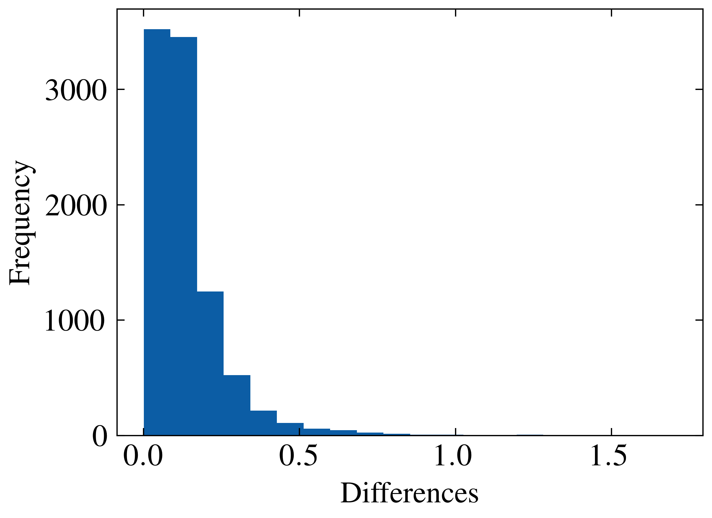
(a) AT

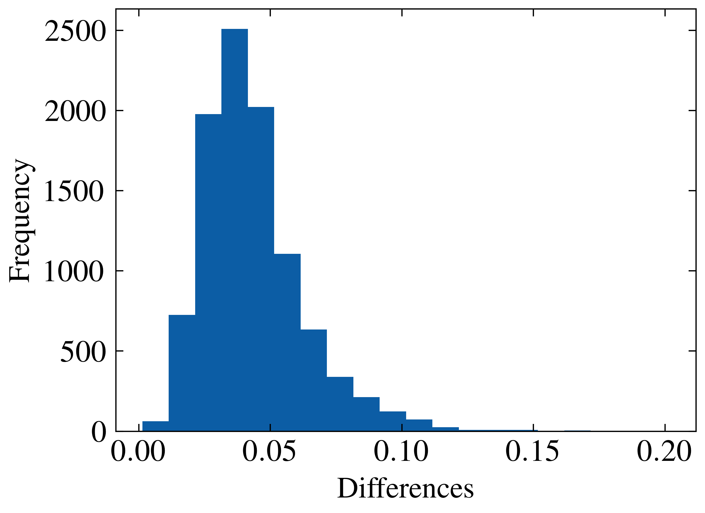
(b) IG-NORM

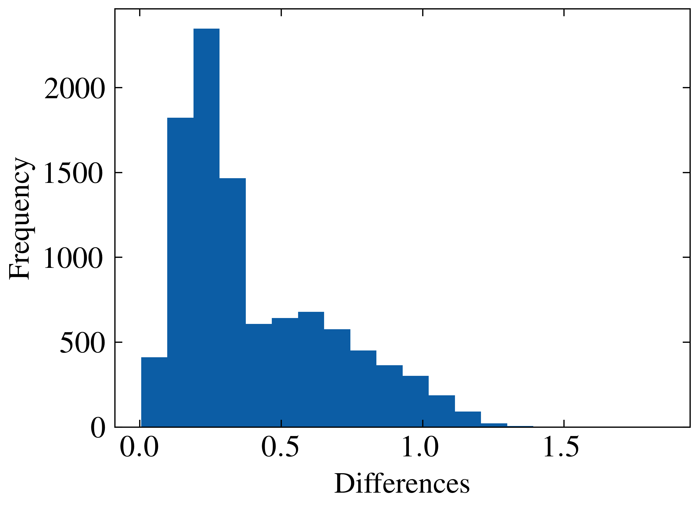
(c) AdvAAT

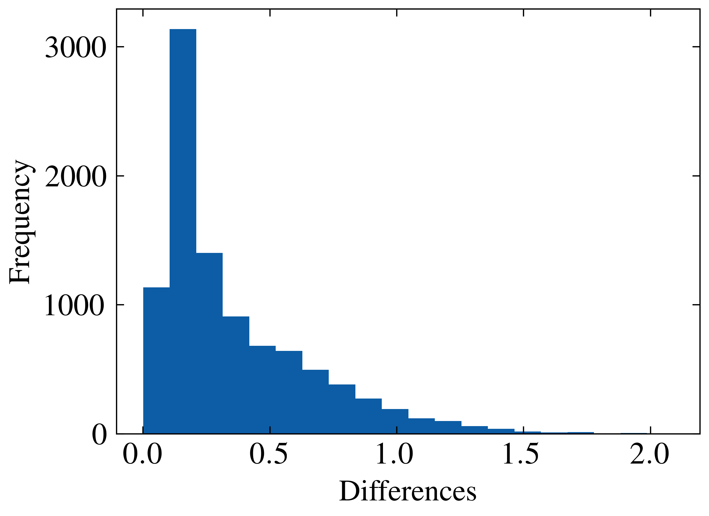
(d) ART

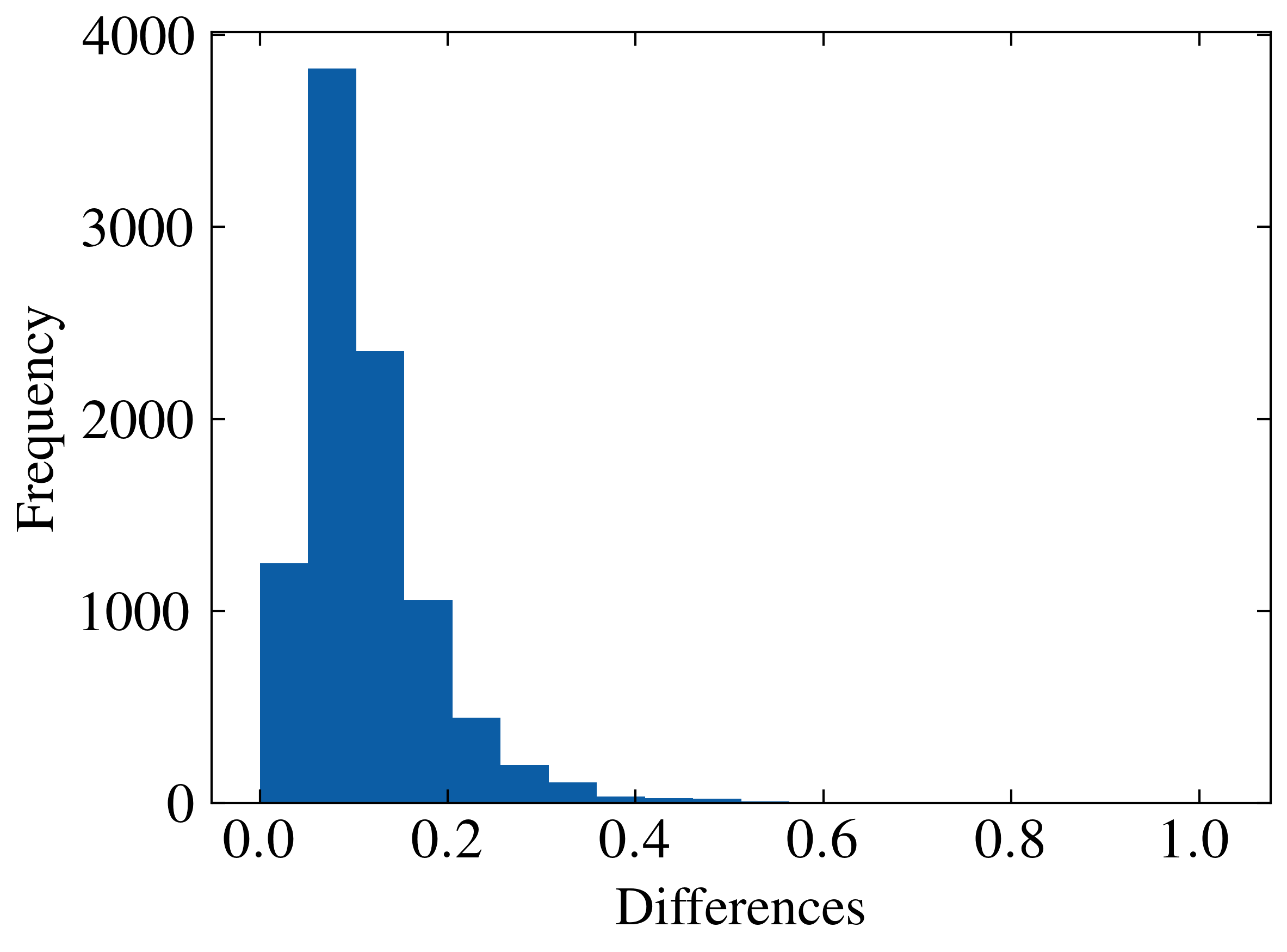
(e) TRADES

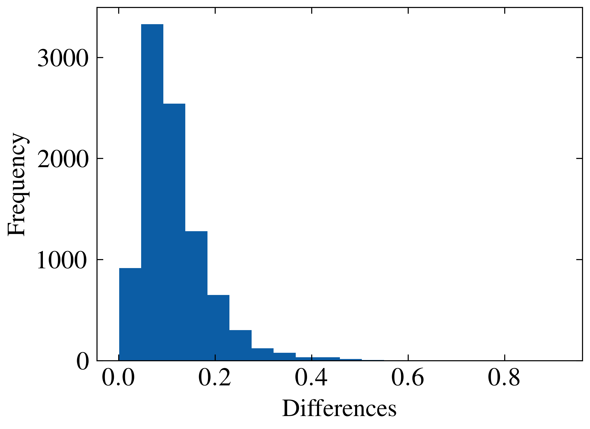
(f) TRADES+IGR

Figure 8: Distributions of differences between computed bounds and attribution differences from CIFAR-10.

Table 9: Evaluation of upper bounds with the label constraint on Flower dataset. The numbers in the brackets indicate the percentages that attacked attribution is outside the $T_{e}$.

	$\ell_{2}$					$\ell_{\infty}$
	$\widehat{T}_{e}$	$T_{e}$	$T^{\prime}_{e}$	$\widehat{T}_{c}$($\deg$)	$T_{c}$($\deg$)	$\widehat{T}_{e}$	$T_{e}$	$\widehat{T}_{c}$($\deg$)	$T_{c}$($\deg$)
AT	0.0170	0.0341 [2.17%]	0.0447	1.3165	1.9806	0.0238	0.4100	2.1937	13.4811
AdvAAT	0.0295	0.1424 [0.00%]	0.1424	1.5568	2.2835	0.0472	0.1025	1.4130	11.8732
TRADES	0.0220	0.0534 [0.72%]	0.0592	1.3383	3.1567	0.0182	0.1081	3.3887	11.9829
TRADES+IGR	0.0080	0.0219 [0.72%]	0.0262	0.8870	2.1255	0.0242	0.2873	1.5930	12.5584

Table 10: Evaluation of upper bounds with the label constraint on ImageNet. The numbers in the brackets indicate the percentages that attacked attribution is outside the $T_{e}$.

	$\ell_{2}$					$\ell_{\infty}$
	$\widehat{T}_{e}$	$T_{e}$	$T^{\prime}_{e}$	$\widehat{T}_{c}$($\deg$)	$T_{c}$($\deg$)	$\widehat{T}_{e}$	$T_{e}$	$\widehat{T}_{c}$($\deg$)	$T_{c}$($\deg$)
CE	0.1049	0.1923[3.06%]	0.2365	7.7959	8.0933	0.3148	0.7399	3.8227	10.9339
AT	0.1077	0.1588[3.32%]	0.5221	3.4773	5.1797	0.1974	0.2226	0.3455	8.7333

D.3 Evaluation of upper bounds under $\ell_{2}$-norm and $\ell_{\infty}$-norm constraints on larger size images.

The proposed method is also scalable to larger size images. In this subsection, we provide experimental results on Flower [20], which contains images of size of $128\times 128\times 3$, and a subset of ImageNet [5] containing 5,000 randomly chosen images with size of $224\times 224\times 3$. We choose $\varepsilon=0.1$ for $\ell_{2}$ and $\varepsilon=8/255$ for $\ell_{\infty}$ cases to compute the theoretical upper bounds $T_{e}$ and $T_{c}$, as well as the modified bound $T^{\prime}_{e}$, as introduced in Sec. 5. The sample distance $\widehat{T}_{e}$ and $\widehat{T}_{c}$ are computed from the mean of distances between perturbed and original attributions, where PGD-20 is used as $\ell_{2}$ attack and 200-step IFIA is used as $\ell_{\infty}$ attack. In paricular, since the baseline attribution robustness methods do not scale up to ImageNet, we only provide results using standard training and adversarial training to illustrate the scalability of our method. The results are presented in Tabs. 9 and 10.

We notice that the theoretical bounds are all valid for larger size images, where all angular and modified Euclidean bound effective bound the maximum discrepancy of perturbed attributions. It worths noting that the computation costs of the values for the upper bound in $\ell_{2}$-norm constrained case become heavier for high-dimensional images due to the computation of eigenvalues for large matrices. For $\ell_{\infty}$-norm case, these eigenvalue computations have been avoided. We will study the scalability of our methods under $\ell_{2}$-norm constraint in future work.

Appendix E Alternative formulation of upper bound to the worst-case attribution deviations

The formulation of Eq. 1 can be rewritten in an equivalent form to find the maximum $\varepsilon$ subject to the attribution difference under certain threshold $\omega$. Formally, the formulation can be written as

$$\max \varepsilon$$ (48)

s.t. $$D(g^{y}({\bm{x}}),g^{y}({\bm{x}}+\bm{\delta}))\leq\omega$$

$$\|\bm{\delta}\|_{p}\leq\varepsilon$$

$$\operatorname*{arg\,max}_{k}f_{k}({\bm{x}})=\operatorname*{arg\,max}_{k}f_{k}({\bm{x}}+\bm{\delta})$$

Under the above formulation, we can use the theoretical bound derived using Eq. 1 to find the corresponding optimal $\varepsilon$. For the $\ell_{2}$-norm case with or without the label constraint, when $D(\cdot,\cdot)$ is the $\ell_{2}$ distance, the maximum $\varepsilon$ can be computed using the upper bound $\xi_{max}\varepsilon$ derived in Theorem 1,

$$\max_{\bm{\delta}}\|g^{y}({\bm{x}}+\bm{\delta})-g^{y}({\bm{x}})\|_{2}=\xi_{max}\varepsilon\leq\omega$$ (49)

$$\Rightarrow\varepsilon\leq\frac{\omega}{\xi_{max}}$$ (50)

Similarly, the maximum $\varepsilon$ when $D(\cdot,\cdot)$ is cosine distance can be derived using Corollary 2 as

$$\max_{\bm{\delta}}D_{c}(g^{y}({\bm{x}}+\bm{\delta}),g^{y}({\bm{x}}))=1-\sqrt{1-\frac{\xi_{max}\varepsilon}{\|g^{y}({\bm{x}})\|_{2}^{2}}}\leq\omega$$ (51)

$$\Rightarrow\varepsilon\leq\frac{\|g({\bm{x}})\|_{2}^{2}}{\xi_{max}}\left(1-(1-\omega)^{2}\right)$$ (52)

The maximum $\varepsilon$ for the $\ell_{\infty}$ constraint case with and without the label constraint can be also derived in the same way using the relaxed upper bound in Theorem 2. Since the Kendall’s rank correlation is discontinuous, researchers proposed to use cosine similarity and $\ell_{p}$ distance to measure the similarity/dissimilarity between attributions from attacked samples and original samples [32, 4, 3]. Thus, in this work, we derive the bounds for cosine similarity and Euclidean distance.

References

- [1] Sebastian Bach, Alexander Binder, Grégoire Montavon, Frederick Klauschen, Klaus-Robert Müller, and Wojciech Samek. On pixel-wise explanations for non-linear classifier decisions by layer-wise relevance propagation. PloS one, 10(7):e0130140, 2015.
- [2] Umang Bhatt, Alice Xiang, Shubham Sharma, Adrian Weller, Ankur Taly, Yunhan Jia, Joydeep Ghosh, Ruchir Puri, José MF Moura, and Peter Eckersley. Explainable machine learning in deployment. In Proceedings of the 2020 conference on fairness, accountability, and transparency, pages 648–657, 2020.
- [3] Akhilan Boopathy, Sijia Liu, Gaoyuan Zhang, Cynthia Liu, Pin-Yu Chen, Shiyu Chang, and Luca Daniel. Proper network interpretability helps adversarial robustness in classification. In International Conference on Machine Learning, pages 1014–1023. PMLR, 2020.
- [4] Jiefeng Chen, Xi Wu, Vaibhav Rastogi, Yingyu Liang, and Somesh Jha. Robust attribution regularization. In Advances in Neural Information Processing Systems, pages 14300–14310, 2019.
- [5] Jia Deng, Wei Dong, Richard Socher, Li-Jia Li, Kai Li, and Li Fei-Fei. Imagenet: A large-scale hierarchical image database. In 2009 IEEE conference on computer vision and pattern recognition, pages 248–255. Ieee, 2009.
- [6] Ann-Kathrin Dombrowski, Maximillian Alber, Christopher Anders, Marcel Ackermann, Klaus-Robert Müller, and Pan Kessel. Explanations can be manipulated and geometry is to blame. In Advances in Neural Information Processing Systems, pages 13589–13600, 2019.
- [7] Chris Finlay and Adam M Oberman. Scaleable input gradient regularization for adversarial robustness. arXiv preprint arXiv:1905.11468, 2019.
- [8] Amirata Ghorbani, Abubakar Abid, and James Zou. Interpretation of neural networks is fragile. In Proceedings of the AAAI Conference on Artificial Intelligence, volume 33, pages 3681–3688, 2019.
- [9] Ian J Goodfellow, Jonathon Shlens, and Christian Szegedy. Explaining and harnessing adversarial examples. In International Conference on Learning Representations, 2015.
- [10] Bryce Goodman and Seth Flaxman. European union regulations on algorithmic decision-making and a “right to explanation”. AI magazine, 38(3):50–57, 2017.
- [11] Hongyu Guo, Yongyi Mao, and Richong Zhang. Mixup as locally linear out-of-manifold regularization. In Proceedings of the AAAI Conference on Artificial Intelligence, volume 33, pages 3714–3722, 2019.
- [12] Adam Ivankay, Ivan Girardi, Chiara Marchiori, and Pascal Frossard. FAR: A general framework for attributional robustness. In 32nd British Machine Vision Conference, BMVC 2021, Online, page 24. BMVA Press, 2021.
- [13] José Jiménez-Luna, Francesca Grisoni, and Gisbert Schneider. Drug discovery with explainable artificial intelligence. Nature Machine Intelligence, 2(10):573–584, 2020.
- [14] Maurice George Kendall. Rank correlation methods. 1948.
- [15] Alex Krizhevsky. Learning multiple layers of features from tiny images. 2009.
- [16] Cassidy Laidlaw, Sahil Singla, and Soheil Feizi. Perceptual adversarial robustness: Defense against unseen threat models. In 9th International Conference on Learning Representations, ICLR 2021, Virtual Event, Austria, May 3-7, 2021. OpenReview.net, 2021.
- [17] Yann LeCun, Corinna Cortes, and CJ Burges. Mnist handwritten digit database. ATT Labs [Online]. Available: http://yann.lecun.com/exdb/mnist, 2, 2010.
- [18] Scott M Lundberg and Su-In Lee. A unified approach to interpreting model predictions. Advances in neural information processing systems, 30, 2017.
- [19] Aleksander Madry, Aleksandar Makelov, Ludwig Schmidt, Dimitris Tsipras, and Adrian Vladu. Towards deep learning models resistant to adversarial attacks. In International Conference on Learning Representations, 2018.
- [20] M-E Nilsback and Andrew Zisserman. A visual vocabulary for flower classification. In 2006 IEEE Computer Society Conference on Computer Vision and Pattern Recognition (CVPR’06), volume 2, pages 1447–1454. IEEE, 2006.
- [21] Panos M Pardalos and Stephen A Vavasis. Quadratic programming with one negative eigenvalue is np-hard. Journal of Global optimization, 1(1):15–22, 1991.
- [22] Chongli Qin, James Martens, Sven Gowal, Dilip Krishnan, Krishnamurthy Dvijotham, Alhussein Fawzi, Soham De, Robert Stanforth, and Pushmeet Kohli. Adversarial robustness through local linearization. Advances in Neural Information Processing Systems, 32, 2019.
- [23] Anindya Sarkar, Anirban Sarkar, and Vineeth N Balasubramanian. Enhanced regularizers for attributional robustness. In Proceedings of the AAAI Conference on Artificial Intelligence, volume 35, pages 2532–2540, 2021.
- [24] Rory Sayres, Ankur Taly, Ehsan Rahimy, Katy Blumer, David Coz, Naama Hammel, Jonathan Krause, Arunachalam Narayanaswamy, Zahra Rastegar, Derek Wu, et al. Using a deep learning algorithm and integrated gradients explanation to assist grading for diabetic retinopathy. Ophthalmology, 126(4):552–564, 2019.
- [25] Avanti Shrikumar, Peyton Greenside, and Anshul Kundaje. Learning important features through propagating activation differences. In International Conference on Machine Learning, pages 3145–3153. PMLR, 2017.
- [26] Avanti Shrikumar, Peyton Greenside, Anna Shcherbina, and Anshul Kundaje. Not just a black box: Learning important features through propagating activation differences. arXiv preprint arXiv:1605.01713, 2016.
- [27] Carl-Johann Simon-Gabriel, Yann Ollivier, Leon Bottou, Bernhard Schölkopf, and David Lopez-Paz. First-order adversarial vulnerability of neural networks and input dimension. In International Conference on Machine Learning, pages 5809–5817. PMLR, 2019.
- [28] Karen Simonyan, Andrea Vedaldi, and Andrew Zisserman. Deep inside convolutional networks: Visualising image classification models and saliency maps. In 2nd International Conference on Learning Representations, ICLR 2014, Banff, AB, Canada, April 14-16, 2014, Workshop Track Proceedings, 2014.
- [29] Amitojdeep Singh, Sourya Sengupta, and Vasudevan Lakshminarayanan. Explainable deep learning models in medical image analysis. Journal of Imaging, 6(6):52, 2020.
- [30] Mayank Singh, Nupur Kumari, Puneet Mangla, Abhishek Sinha, Vineeth N Balasubramanian, and Balaji Krishnamurthy. Attributional robustness training using input-gradient spatial alignment. In Computer Vision–ECCV 2020: 16th European Conference, Glasgow, UK, August 23–28, 2020, Proceedings, Part XXVII 16, pages 515–533. Springer, 2020.
- [31] Mukund Sundararajan, Ankur Taly, and Qiqi Yan. Axiomatic attribution for deep networks. In International Conference on Machine Learning, pages 3319–3328. PMLR, 2017.
- [32] Fan Wang and Adams Wai-Kin Kong. Exploiting the relationship between kendall’s rank correlation and cosine similarity for attribution protection. In Alice H. Oh, Alekh Agarwal, Danielle Belgrave, and Kyunghyun Cho, editors, Advances in Neural Information Processing Systems, 2022.
- [33] Zifan Wang, Haofan Wang, Shakul Ramkumar, Piotr Mardziel, Matt Fredrikson, and Anupam Datta. Smoothed geometry for robust attribution. In Advances in Neural Information Processing Systems, volume 33, pages 13623–13634. Curran Associates, Inc., 2020.
- [34] Han Xiao, Kashif Rasul, and Roland Vollgraf. Fashion-mnist: a novel image dataset for benchmarking machine learning algorithms. arXiv preprint arXiv:1708.07747, 2017.
- [35] Yao-Yuan Yang, Cyrus Rashtchian, Hongyang Zhang, Russ R Salakhutdinov, and Kamalika Chaudhuri. A closer look at accuracy vs. robustness. Advances in neural information processing systems, 33:8588–8601, 2020.
- [36] Matthew D Zeiler and Rob Fergus. Visualizing and understanding convolutional networks. In European conference on computer vision, pages 818–833. Springer, 2014.
- [37] Hongyang Zhang, Yaodong Yu, Jiantao Jiao, Eric Xing, Laurent El Ghaoui, and Michael Jordan. Theoretically principled trade-off between robustness and accuracy. In International Conference on Machine Learning, pages 7472–7482. PMLR, 2019.
- [38] Linjun Zhang, Zhun Deng, Kenji Kawaguchi, Amirata Ghorbani, and James Zou. How does mixup help with robustness and generalization? In 9th International Conference on Learning Representations, ICLR 2021, Virtual Event, Austria, May 3-7, 2021. OpenReview.net, 2021.
- [39] Luisa M. Zintgraf, Taco S. Cohen, Tameem Adel, and Max Welling. Visualizing deep neural network decisions: Prediction difference analysis. In International Conference on Learning Representations, ICLR 2017. OpenReview.net, 2017.