Posterior Robustness with Milder Conditions: Contamination Models Revisited

Abstract

Robust Bayesian linear regression is a classical but essential statistical tool. Although novel robustness properties of posterior distributions have been proved recently under a certain class of error distributions, their sufficient conditions are restrictive and exclude several important situations. In this work, we revisit a classical two-component mixture model for response variables, also known as contamination model, where one component is a light-tailed regression model and the other component is heavy-tailed. The latter component is independent of the regression parameters, which is crucial in proving the posterior robustness. We obtain new sufficient conditions for posterior (non-)robustness and reveal non-trivial robustness results by using those conditions. In particular, we find that even the Student-$t$ error distribution can achieve the posterior robustness in our framework. A numerical study is performed to check the Kullback-Leibler divergence between the posterior distribution based on full data and that based on data obtained by removing outliers.

Keywords: heavy-tailed distribution; posterior robustness; two-component mixture

Introduction

Bayesian posterior robustness (O’Hagan, 1979) and related topics have long been studied (e.g., West, 1984; Andrade and O’Hagan, 2006, 2011; O’Hagan and Pericchi, 2012). There, one of the most important objectives is to perform posterior analysis using moderate observations only and discarding outliers that are not related to the parameters of interest. Because the task of manually detecting or determining outliers is difficult in general, robust models are desired under which the effects of outliers are automatically removed.

Although many robust regression models have been proposed in the literature, few works (e.g., O’Hagan, 1979) have given theoretical justifications to those models. In fact, it is only recently that Desgagné (2013, 2015) and Gagnon et al. (2019) have proved posterior robustness for scale, location-scale, and regression models, respectively. Here, posterior densities are said to be robust if they converge to the corresponding conditional densities of parameters based only on non-outliers as the absolute values of outliers tend to infinity. Since then, posterior robustness has been established in various practically important settings; Hamura et al. (2022) obtained robustness results for regressions with shrinkage priors, whereas Hamura et al. (2021) considered a case of integer-valued observation.

In proving the posterior robustness, Gagnon et al. (2019) and Hamura et al. (2022) considered the following model; with observations $y_{1},\dots,y_{n}$, $p$-dimensional covariate vectors ${\text{\boldmath$x$}}_{1},\dots,{\text{\boldmath$x$}}_{n}$, regression coefficients ${\text{\boldmath$\beta$}}\in\mathbb{R}^{p}$ and a scale parameter ${\sigma}\in(0,\infty)$, they assume

$$y_{i}\sim f((y_{i}-{{\text{\boldmath$x$}}_{i}}^{\top}{\text{\boldmath$\beta$}})/{\sigma})/{\sigma},\ \ \ \ i=1,\ldots,n,$$ (1)

for some error density $f$ and prior $({\text{\boldmath$\beta$}},{\sigma})\sim\pi({\text{\boldmath$\beta$}},{\sigma})$. In their proof, it is crucial to assume the log-regularly varying error density, which has tails heavier than the Student’s $t$-distributions, to ensure posterior robustness. If $f$ is the Student’s $t$-distribution, the posterior is not robust (Gagnon and Hayashi, 2023). These theoretical findings imply the superiority of log-regularly varying error density to the Student’s $t$-distributions. However, it has also been reported that the Student’s $t$-error distribution is fairly competitive in posterior inference in several numerical studies (Hamura et al., 2022).

In this paper, we revisit the following classical two-component mixture regression model, also known as the contamination model:

$$y_{i}\sim(1-s)f_{0}((y_{i}-{{\text{\boldmath$x$}}_{i}}^{\top}{\text{\boldmath$\beta$}})/{\sigma})/{\sigma}+sf_{1}(y_{i})\text{,}\ \ \ \ i=1,\ldots,n,$$ (2)

where $({\text{\boldmath$\beta$}},{\sigma})\sim\pi({\text{\boldmath$\beta$}},{\sigma})$ and $s\in(0,1)$ is a prior probability that an observation becomes an outlier. The first density, $f_{0}$, has thinner tails and is typically the standard normal distribution. The second density, $f_{1}$, is a heavy-tailed distribution, such as Student’s $t$-distribution, and expected to accommodate outliers. One notable feature of the above model is that the second term is completely independent of the parameters $({\text{\boldmath$\beta$}},{\sigma})$. This is a significant difference from the classical two-component mixtures in Box and Tiao (1968) and subsequent research (Tak et al., 2019; Silva et al., 2020), where the second component is also scaled by observational standard error $\sigma$.

Under the model (2), we show that the posterior is robust if $\pi({\sigma})$, the marginal prior for ${\sigma}$, has tails sufficiently lighter than those of the error density $f_{1}$. When $f_{1}$ is log-regularly varying, then most of prior distributions can satisfy this sufficient condition for robustness. Furthermore, we prove that the sufficient condition on the tails of $\pi({\sigma})$ is “nearly” necessary as well; if the error distribution is not log-regularly varying and has lighter tails than $\pi({\sigma})$, then the posterior is not robust. With these conditions, we can identify the posterior (non)-robustness for most of the error and prior distributions used in the regression models.

Our result can also explain the gap between the non-robustness of the Student $t$-distribution in model (1) and its success in posterior inference in numerical studies. For simplicity, assume that only the first observation, $y_{1}$, is outlying and let $|y_{1}|\to\infty$. Then, under the model (1) with $f(y)\propto|y|^{-1-{\alpha}}$ as $|y|\to\infty$ for ${\alpha}>0$ (Student’s $t$-distribution with ${\alpha}$ degree-of-freedom), it holds that

$$p({\text{\boldmath$\beta$}},{\sigma}|{\text{\boldmath$y$}}) \propto\pi({\text{\boldmath$\beta$}},{\sigma}){f((y_{1}-{{\text{\boldmath$x$}}_{1}}^{\top}{\text{\boldmath$\beta$}})/{\sigma})\over f(y_{1}){\sigma}}\prod_{i=2}^{n}{f((y_{i}-{{\text{\boldmath$x$}}_{i}}^{\top}{\text{\boldmath$\beta$}})/{\sigma})\over{\sigma}}{}$$

$$\to\pi({\text{\boldmath$\beta$}},{\sigma}){\sigma}^{{\alpha}}\prod_{i=2}^{n}{f((y_{i}-{{\text{\boldmath$x$}}_{i}}^{\top}{\text{\boldmath$\beta$}})/{\sigma})\over{\sigma}}{}$$

as $|y_{1}|\to\infty$. This limit is the product of the posterior density without $y_{1}$ and factor ${\sigma}^{{\alpha}}$. In other words, the Student’s $t$-distribution can never achieve the posterior robustness. By contrast, under the model (2), we have

$$p({\text{\boldmath$\beta$}},{\sigma}|{\text{\boldmath$y$}}) \propto\pi({\text{\boldmath$\beta$}},{\sigma})\Big{\{}{1-s\over s}{f_{0}((y_{1}-{{\text{\boldmath$x$}}_{1}}^{\top}{\text{\boldmath$\beta$}})/{\sigma})\over{\sigma}f_{1}(y_{1})}+1\Big{\}}\prod_{i=2}^{n}\Big{\{}(1-s){f_{0}((y_{i}-{{\text{\boldmath$x$}}_{i}}^{\top}{\text{\boldmath$\beta$}})/{\sigma})\over{\sigma}}+sf_{1}(y_{i})\Big{\}}{}$$

$$\to\pi({\text{\boldmath$\beta$}},{\sigma})\prod_{i=2}^{n}\Big{\{}(1-s){f_{0}((y_{i}-{{\text{\boldmath$x$}}_{i}}^{\top}{\text{\boldmath$\beta$}})/{\sigma})\over{\sigma}}+sf_{1}(y_{i})\Big{\}}{}$$

as $|y_{1}|\to\infty$, provided that $f_{1}$ has sufficiently heavier tails than $f_{0}$. This is precisely the posterior without $y_{1}$, for which we confirm the posterior robustness. Here, the main difference from the model (1) is that the second component $f_{1}$ of (2) does not involve the parameters $({\text{\boldmath$\beta$}},\sigma)$ of the first component. Thanks to this difference, outliers are not linked to any of parameters $({\text{\boldmath$\beta$}},{\sigma})$ in this model and therefore have no effects on the joint posterior distribution of $({\text{\boldmath$\beta$}},{\sigma})$, as long as $f_{1}$ has heavier tails than $f_{0}$. This observation applies to the general case of multiple outliers, as will be seen below.

The remainder of this paper is organized as follows. In Section 2, sufficient conditions and necessary conditions for posterior robustness are given. In Section 3, a numerical example is given, in which we see that the Kullback-Leibler divergence between the target and available posteriors can diverge or converge to $0$ in some cases. Proofs are given in the Supplementary Material.

Contamination Models and Posterior Robustness

Suppose that we observe

$$y_{i}\sim(1-s){\rm{N}}(y_{i}|{{\text{\boldmath$x$}}_{i}}^{\top}{\text{\boldmath$\beta$}},{\sigma}^{2})+sf_{1}(y_{i}){}$$

for $i=1,\dots,n$, where ${\text{\boldmath$x$}}_{i}$ are continuous continuous explanatory variables and where ${\text{\boldmath$\beta$}}=({\beta}_{k})_{k=1}^{p}\in\mathbb{R}^{p}$ and ${\sigma}\in(0,\infty)$ are parameters of interest following a prior distribution $\pi({\text{\boldmath$\beta$}},{\sigma})$. Here, $f_{1}(\cdot)$ is an error density, and $s\in(0,1)$ is a prior probability that observation is generated from $f_{1}$.

Following the work of Desgagné (2015), let ${\cal K},{\cal L}\subset\{1,\dots,n\}$ satisfy ${\cal K}\cup{\cal L}=\{1,\dots,n\}$, ${\cal K}\cap{\cal L}=\emptyset$, and ${\cal K},{\cal L}\neq\emptyset$. Suppose that $a_{i}\in\mathbb{R}$, $b_{i}\neq 0$, and $y_{i}=a_{i}+b_{i}{\omega}$, ${\omega}\to\infty$, for $i\in{\cal L}$, such that ${\cal L}$ represents the set of indices of outlying observations. We say that the posterior is robust to outliers under the above model if $p({\text{\boldmath$\beta$}},{\sigma}|{\text{\boldmath$y$}})\to p({\text{\boldmath$\beta$}},{\sigma}|{\text{\boldmath$y$}}_{{\cal K}})$ as ${\omega}\to\infty$, where ${\text{\boldmath$y$}}=(y_{i})_{i=1}^{n}$, ${\text{\boldmath$y$}}_{{\cal K}}=(y_{i})_{i\in{\cal K}}$, and ${\text{\boldmath$y$}}_{{\cal L}}=(y_{i})_{i\in{\cal L}}$.

To derive conditions for posterior robustness, we limit the class of prior distributions for $({\text{\boldmath$\beta$}},{\sigma})$. Suppose that

$$\pi({\text{\boldmath$\beta$}}|{\sigma})={\pi({\text{\boldmath$\beta$}},{\sigma})\over\pi({\sigma})}\leq M\prod_{k=1}^{p}\Big{\{}{1\over{\sigma}}{(|{\beta}_{k}|/{\sigma})^{{\kappa}-1}\over(1+|{\beta}_{k}|/{\sigma})^{{\kappa}+\nu}}\Big{\}},$$ (3)

for some $\nu>0$, $0<{\kappa}\leq 1$ and $M>0$, where $\pi({\sigma})=\int_{\mathbb{R}^{p}}\pi({\text{\boldmath$\beta$}},{\sigma})d{\text{\boldmath$\beta$}}$. That is, the ratio of the prior density and some double-sided scaled-beta density (with spike at the origin) must be bounded uniformly by some constant. This condition is satisfied by most of the conditionally independent priors that are commonly used in practice. Examples include shrinkage priors, such as the horseshoe prior (Carvalho et al., 2009, 2010), as well as the normal priors. The condition is also satisfied by some multivariate priors for dependent $\beta$, including the multivariate normal prior.

Likewise, we assume the error distributions, $f_{1}$, are bounded as

$$f_{1}(y) \geq{1\over M^{\prime}}{1\over(1+|y|)^{1+{\alpha}}}{1\over\{1+\log(1+|y|)\}^{1+{\gamma}}},$$ (4)

for some ${\alpha}\geq 0$, ${\gamma}\geq-1$ and $M^{\prime}>0$. The class of distributions that satisfy this condition includes Student’s $t$-distributions (${\alpha}>0$ and ${\gamma}=-1$) and log-regularly varying distributions (${\alpha}=0$ and ${\gamma}>0$).

The following theorem gives a sufficient condition for the posterior to be robust.

Theorem 1.

Suppose that conditions (3) and (4) are satisfied for $\nu>{\alpha}$. Also, suppose that

$$E[{\sigma}^{|{\cal L}|{\alpha}+\rho}]<\infty$$ (5)

for some $\rho>0$. Then the posterior is robust to outliers under our model; that is, we have

$$\lim_{{\omega}\to\infty}p({\text{\boldmath$\beta$}},{\sigma}|{\text{\boldmath$y$}})=p({\text{\boldmath$\beta$}},{\sigma}|{\text{\boldmath$y$}}_{{\cal K}}){}$$

at each $({\text{\boldmath$\beta$}},{\sigma})\in\mathbb{R}^{p}\times(0,\infty)$.

The moment condition for $\pi({\sigma})$ in (5) could be a strong requirement, especially when $\alpha>0$ and multiple outliers are expected. Next, we prove that the posterior robustness does not hold if this moment condition is not satisfied, in addition that the error density tails are not sufficiently heavily tailed.

Theorem 2.

Let $h\colon\mathbb{R}^{p}\to(0,\infty)$ be a probability density and suppose that $\pi({\text{\boldmath$\beta$}}|{\sigma})=h({\text{\boldmath$\beta$}}/{\sigma})/{\sigma}^{p}$. Let ${\alpha}>0$ and suppose that

$$f_{1}(y) \leq M^{\prime}{1\over(1+|y|)^{1+{\alpha}}}{}$$

for all $y\in\mathbb{R}$ for some $M^{\prime}>0$. Suppose that

$$\pi({\sigma})\geq(1/{\widetilde{M}})/{\sigma}^{|{\cal L}|{\alpha}+1-\rho}$$ (6)

for all ${\sigma}>1$ for some ${\widetilde{M}}>0$ and $0<\rho<1$. Then we have

$$\lim_{{\omega}\to\infty}p({\text{\boldmath$\beta$}},{\sigma}|{\text{\boldmath$y$}})=0{}$$

at each $({\text{\boldmath$\beta$}},{\sigma})\in\mathbb{R}^{p}\times(0,\infty)$.

Clearly, under the assumptions of Theorem 2, the posterior does not converge in the usual sense. Indeed, we see in the next section that the Kullback-Leibler divergence between $p({\text{\boldmath$\beta$}},{\sigma}|{\text{\boldmath$y$}}_{{\cal K}})$ and $p({\text{\boldmath$\beta$}},{\sigma}|{\text{\boldmath$y$}})$ diverges in such a situation.

From Theorems 1 and 2, we can determine whether a prior $\pi({\sigma})$ yields a robust posterior or not in most cases. Suppose that ${\text{\boldmath$\beta$}}/{\sigma}$ and ${\sigma}$ are independent and that (3) holds. Suppose that equality holds in (4). Then, if we use a gamma prior for ${\sigma}^{2}$, the moment condition in (5) is always satisfied; hence the posterior is robust regardless of the choice of ${\alpha}$. If we use an inverse gamma prior or a scaled beta prior for ${\sigma}^{2}$, either (5) or (6) is satisfied, depending on the hyperparameters. That is, there exists a threshold separating robust and non-robust cases. These observations are summarized in Table 1.

Table 1: Priors and conditions in Theorem 1 and 2

Prior for $\sigma^{2}$	Density $\pi({\sigma})d{\sigma}$	Condition (5)	Condition (6)
		for robustness	for non-robustness
Inverse-gamma:	$(1/{\sigma}^{2A+1})\exp(-B/{\sigma}^{2})$	$2A>|{\cal L}|{\alpha}$	$2A<|{\cal L}|{\alpha}$
$\mathrm{IG}(A,B)$
Gamma: $\mathrm{Ga}(C,D)$	${\sigma}^{2C-1}\exp(-D{\sigma}^{2})$	✓	NA
Scaled-beta:	${\sigma}^{2E-1}/(1+{\sigma}^{2})^{E+F}$	$2F>|{\cal L}|{\alpha}$	$2F<|{\cal L}|{\alpha}$
$\mathrm{SB}(E,F)$

The sufficient conditions obtained in this study differ from those in Gagnon et al. (2019) and Hamura et al. (2022) not only in the model specification given in (1) and (2) but also in the requirement of the error and prior densities. Table 2 summarizes the sufficient conditions for posterior robustness in the literature and Theorem 1. It is worth emphasizing that, in Theorem 1, we do not make any assumption directly on $|{\cal L}|$, the number of outliers. In proving the posterior robustness, it is inevitable to control the number of the indices $i\in{\cal L}$ for which $|y_{i}-{{\text{\boldmath$x$}}_{i}}^{\top}{\text{\boldmath$\beta$}}|$ is outlying and the number of the indices $i\in{\cal K}$ for which $|y_{i}-{{\text{\boldmath$x$}}_{i}}^{\top}{\text{\boldmath$\beta$}}|$ is close to $0$. These numbers are further studied in our Lemma 1, which enables the proof of posterior robustness without any assumption on $|{\cal L}|$. For details, see the Supplemetary Materials. In addition, as pointed out in the introduction, our model allows $f_{1}$ not to be log-regular varying in proving the posterior robustness, which is also significantly different from the settings in the literature. However, we also note that these conditions are not nested in one another. For example, the conditions in Gagnon et al. (2019) cover the improper prior for $({\text{\boldmath$\beta$}},{\sigma})$.

Table 2: Sufficient conditions of model components for robustness

	Number of	Error density	Prior density $\pi({\text{\boldmath$\beta$}},{\sigma})$
	outliers $|{\cal L}|$	tails ($f$ or $f_{1}$)	Density bounds	Moments	Improper
Gagnon et al.	$|{\cal K}|\geq|{\cal L}|+2p-1$	LRVD	$\max\{1,1/{\sigma}\}$	–	✓
(2019)
Hamura et al.	$|{\cal K}|\geq|{\cal L}|+p$	LRVD	$\displaystyle\sup_{t\in\mathbb{R}}|t|\pi_{{\beta}}(t)<\infty$	$E[{\sigma}^{-n}]<\infty$	NA
(2020)
Theorem 1	Not needed	${1\over(1+|y|)^{1+{\alpha}}}$	$\prod\limits_{k=1}^{p}{(|{\beta}_{k}|/{\sigma})^{{\kappa}-1}/{\sigma}\over(1+|{\beta}_{k}|/{\sigma})^{{\kappa}+\nu}}$	$E[{\sigma}^{|{\cal L}|{\alpha}+\rho}]<\infty$	NA
of this study

Numerical Examples

Here, we numerically calculate the Kullback-Leibler (KL) divergence of the target posterior distribution $p({\text{\boldmath$\beta$}},{\sigma}|{\text{\boldmath$y$}}_{{\cal K}})$ from the available posterior distribution $p({\text{\boldmath$\beta$}},{\sigma}|{\text{\boldmath$y$}})$, which is given by

$${\rm{KL}}=\int_{\mathbb{R}^{p}\times(0,\infty)^{p}}p({\text{\boldmath$\beta$}},{\sigma}|{\text{\boldmath$y$}}_{{\cal K}})\log{p({\text{\boldmath$\beta$}},{\sigma}|{\text{\boldmath$y$}}_{{\cal K}})\over p({\text{\boldmath$\beta$}},{\sigma}|{\text{\boldmath$y$}})}d({\text{\boldmath$\beta$}},{\sigma})\text{.}{}$$

We use the conjugate normal-inverse gamma prior:

$$\pi({\text{\boldmath$\beta$}},{\sigma}) ={2B^{A}\over{\Gamma}(A)}{1\over{\sigma}^{2A+1}}\exp\Big{(}-{B\over{\sigma}^{2}}\Big{)}{1\over(2\pi)^{p/2}C^{p}{\sigma}^{p}}\exp\Big{(}-{\|{\text{\boldmath$\beta$}}\|^{2}\over 2C^{2}{\sigma}^{2}}\Big{)}\text{,}{}$$

where $A,B,C>0$. Under this prior, the posterior becomes a finite mixture of known distributions and analytically and numerically tractable. We consider the following two error densities:

$$f_{1}^{\rm{light}}(y)={{\alpha}/2\over(1+|y|)^{1+{\alpha}}}\text{,}\quad y\in\mathbb{R}\text{,}{}$$

$$f_{1}^{\rm{heavy}}(y)={{\gamma}/2\over 1+|y|}{1\over\{1+\log(1+|y|)\}^{1+{\gamma}}}\text{,}\quad y\in\mathbb{R}\text{,}{}$$

where ${\alpha},{\gamma}>0$. The first error distribution, $f_{1}^{\rm{light}}$, is the double-sided scale-beta distribution, whose tail behavior is equivalent to that of Student’s $t$-distribution. The second error distribution, $f_{1}^{\rm{heavy}}$, is the unfolded version of the log-Pareto distribution of Cormann and Reiss (2009).

As an example, we set ${\alpha}=3$ and ${\gamma}=3/2$, $B=C=1$, $s=1/10$, ${\text{\boldmath$y$}}=(1,2,3,4,{\omega})^{\top}$, ${\omega}\in\{10^{1},10^{2},10^{3},10^{4},10^{5}\}$, and

$$\begin{pmatrix}{{\text{\boldmath$x$}}_{1}}^{\top}\\ \vdots\\ {{\text{\boldmath$x$}}_{5}}^{\top}\end{pmatrix} =\begin{pmatrix}1&2-1/3\\ 1&2-1/4\\ 1&2-1/5\\ 1&2-1/6\\ 1&2-1/7\end{pmatrix}\text{.}{}$$

In this example, $n=5$, $p=2$, and ${\cal K}=\{1,\dots,4\}$ and ${\cal L}=\{5\}$. For the two cases $A=1/10$ and $A=2$, and for each of the error distributions $f_{1}^{\rm{light}}$ and $f_{1}^{\rm{heavy}}$, we obtain the Monte Carlo approximation of the KL divergence by using 1,000 samples from the posterior distributions. The results are summarized in Figure 1. It is clearly seen that the KL divergence does not converge to $0$ when $f_{1}=f_{1}^{\rm{light}}$ and $A=1/10$, since the condition of Theorem 2 is satisfied and the posterior is not convergent. In the other three cases, where the sufficient condition of Theorem 1 is satisfied, the KL divergence converges to $0$.

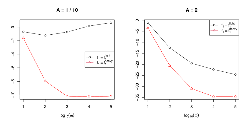
Figure 1: The logarithm of the KL divergence between $p({\text{\boldmath$\beta$}},{\sigma}|{\text{\boldmath$y$}}_{{\cal K}})$ and $p({\text{\boldmath$\beta$}},{\sigma}|{\text{\boldmath$y$}})$ for ${\omega}=10^{1},10^{2},10^{3},10^{4},10^{5}$.

Next, under the same setting, Figure 2 shows the posterior and predictive distributions of ${\beta}_{1}+{\tilde{x}}_{2}{\beta}_{2}$ and ${\tilde{y}}\sim(1-s)f_{0}(\{{\tilde{y}}-({\beta}_{1}+{\tilde{x}}_{2}{\beta}_{2})\}/{\sigma})/{\sigma}+sf_{1}({\tilde{y}})$ given $y$ with ${\omega}=10^{2}$ for ${\tilde{x}}_{2}\in\{1.5,1.6,\dots,1.9,2.0\}$. When $f_{1}=f_{1}^{\rm{light}}$ and $A=1/10$, the credible intervals become extremely wide since the posterior of $({\text{\boldmath$\beta$}},{\sigma})$ converges to zero. Comparing the two panels for $f_{1}^{\rm{light}}$ and $f_{1}^{\rm{heavy}}$ when $A=2$, it can be seen that the predictive intervals are slightly wider for $f_{1}^{\rm{heavy}}$ than for $f_{1}^{\rm{light}}$, reflecting the difference in the tail behavior of the two error densities.

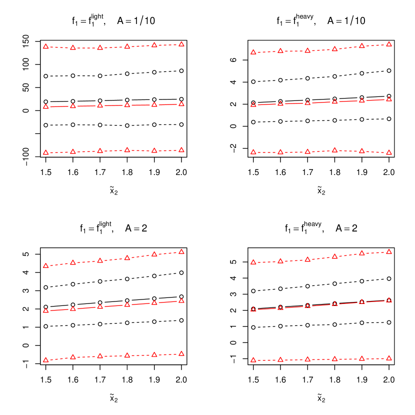
Figure 2: The posterior medians and quantiles of ${\beta}_{1}+{\tilde{x}}_{2}{\beta}_{2}$ (black) and of ${\tilde{y}}$ (red) for ${\tilde{x}}_{2}=1.5,1.6,\dots,1.9,2.0$. Here, we set ${\omega}=10^{2}$.

Supplementary Material for “Posterior Robustness with Milder Conditions: Contamination Models Revisited”

A Basic Lemma

The following result is used in the proof of Theorem 1 of the main text.

Lemma 1.

Let $p\in\mathbb{N}$ and $m,n\in\mathbb{N}$. Let $a_{i}\in\mathbb{R}$, $b_{i}\neq 0$, and ${\text{\boldmath$x$}}_{i}\in\mathbb{R}^{p}$, $i=1,\dots,m$, and $c_{j}\in\mathbb{R}$ and ${\text{\boldmath$z$}}_{j}\in\mathbb{R}^{p}$, $j=1,\dots,n$, be continuous variables such that there is no exact collinearity.

• For any $l\in\mathbb{N}$, there exist ${\delta},{\varepsilon},M>0$ such that for all ${\omega}\geq M$ and all ${\text{\boldmath$\beta$}}\in\mathbb{R}^{p}$, the condition that

  • there exist distinct indices $i_{1},\dots,i_{l}=1,\dots,m$ such that $|a_{i_{1}}+b_{i_{1}}{\omega}-{{\text{\boldmath$x$}}_{i_{1}}}^{\top}{\text{\boldmath$\beta$}}|,\dots,|a_{i_{l}}+b_{i_{l}}{\omega}-{{\text{\boldmath$x$}}_{i_{l}}}^{\top}{\text{\boldmath$\beta$}}|\leq{\varepsilon}{\omega}$

  implies that

  • there exist distinct indices $k_{1},\dots,k_{l}=1,\dots,p$ such that $|{\beta}_{k_{1}}|,\dots,|{\beta}_{k_{l}}|\geq{\delta}{\omega}$.

• Let $c_{j}=0$ and ${\text{\boldmath$z$}}_{j}={\text{\boldmath$e$}}_{-j}^{(p)}$ for $j=-1,\dots,-p$. Let ${\widehat{J}}=\{-1,\dots,-p\}\cup\{1,\dots,n\}$. Let $\eta>0$ be arbitrary. Then for any $1\leq l\leq p$, there exist ${\varepsilon},M>0$ such that for all ${\omega}\geq M$ and all ${\text{\boldmath$\beta$}}\in\mathbb{R}^{p}$, the condition that

  • there exist distinct indices $i_{1},\dots,i_{l}=1,\dots,m$ such that $|a_{i_{1}}+b_{i_{1}}{\omega}-{{\text{\boldmath$x$}}_{i_{1}}}^{\top}{\text{\boldmath$\beta$}}|,\dots,|a_{i_{l}}+b_{i_{l}}{\omega}-{{\text{\boldmath$x$}}_{i_{l}}}^{\top}{\text{\boldmath$\beta$}}|\leq{\varepsilon}{\omega}$

  implies that

  • the set of indices $\{j\in{\widehat{J}}||c_{j}-{{\text{\boldmath$z$}}_{j}}^{\top}{\text{\boldmath$\beta$}}|\leq\eta\}$ has at most $p-l$ elements.

• Let $\eta>0$ and $\overline{{\varepsilon}}>0$ be arbitrary. Then there exist ${\delta}>0$, $0<{\varepsilon}<\overline{{\varepsilon}}$, and $M>0$ such that for all ${\omega}\geq M$,

  $$\mathbb{R}^{p} \subset\Big{(}\bigcap_{i=1}^{m}\{{\text{\boldmath$\beta$}}\in\mathbb{R}^{p}||a_{i}+b_{i}{\omega}-{{\text{\boldmath$x$}}_{i}}^{\top}{\text{\boldmath$\beta$}}|>{\varepsilon}{\omega}\}\Big{)}{}$$

  $$\quad\cup\bigcup_{l=1}^{p}\bigcup_{1\leq i_{1}<\dots<i_{l}\leq m}\Big{(}\Big{(}\bigcap_{i\in\{i_{1},\dots,i_{l}\}}\{{\text{\boldmath$\beta$}}\in\mathbb{R}^{p}||a_{i}+b_{i}{\omega}-{{\text{\boldmath$x$}}_{i}}^{\top}{\text{\boldmath$\beta$}}|\leq{\varepsilon}{\omega}\}\Big{)}{}$$

  $$\quad\cap\Big{(}\bigcap_{i\in\{1,\dots,m\}\setminus\{i_{1},\dots,i_{l}\}}\{{\text{\boldmath$\beta$}}\in\mathbb{R}^{p}||a_{i}+b_{i}{\omega}-{{\text{\boldmath$x$}}_{i}}^{\top}{\text{\boldmath$\beta$}}|>{\varepsilon}{\omega}\}\Big{)}{}$$

  $$\quad\cap\Big{\{}\bigcup_{1\leq k_{1}<\dots<k_{l}\leq p}\bigcap_{k\in\{k_{1},\dots,k_{l}\}}\{{\text{\boldmath$\beta$}}\in\mathbb{R}^{p}||({\text{\boldmath$e$}}_{k}^{(p)})^{\top}{\text{\boldmath$\beta$}}|\geq{\delta}{\omega}\}\Big{\}}{}$$

  $$\quad\cap\Big{[}\Big{(}\bigcap_{j\in{\widehat{J}}}\{{\text{\boldmath$\beta$}}\in\mathbb{R}^{p}||c_{j}-{{\text{\boldmath$z$}}_{j}}^{\top}{\text{\boldmath$\beta$}}|>\eta\}\Big{)}{}$$

  $$\quad\cup\bigcup_{1\leq q\leq p-l}\bigcup_{\begin{subarray}{c}j_{1},\dots,j_{q}\in{\widehat{J}}\\ j_{1}<\dots<j_{q}\end{subarray}}\Big{\{}\Big{(}\bigcap_{j\in\{j_{1},\dots,j_{q}\}}\{{\text{\boldmath$\beta$}}\in\mathbb{R}^{p}||c_{j}-{{\text{\boldmath$z$}}_{j}}^{\top}{\text{\boldmath$\beta$}}|\leq\eta\}\Big{)}{}$$

  $$\quad\cap\Big{(}\bigcap_{j\in{\widehat{J}}\setminus\{j_{1},\dots,j_{q}\}}\{{\text{\boldmath$\beta$}}\in\mathbb{R}^{p}||c_{j}-{{\text{\boldmath$z$}}_{j}}^{\top}{\text{\boldmath$\beta$}}|>\eta\}\Big{)}\Big{\}}\Big{]}\Big{)}\text{.}{}$$

Proof.   For part (i), note that for all ${\varepsilon}>0$, ${\omega}>0$, and ${\text{\boldmath$\beta$}}\in\mathbb{R}^{p}$ and all $i=1,\dots,m$, we have that

$$|a_{i}+b_{i}{\omega}-{{\text{\boldmath$x$}}_{i}}^{\top}{\text{\boldmath$\beta$}}|\leq{\varepsilon}{\omega}\quad\text{if and only if}\quad{{\text{\boldmath$x$}}_{i}}^{\top}{\text{\boldmath$\beta$}}/{\omega}\in[a_{i}/{\omega}+b_{i}\pm{\varepsilon}]\text{.}{}$$

In particular, $|a_{i}+b_{i}{\omega}-{{\text{\boldmath$x$}}_{i}}^{\top}{\text{\boldmath$\beta$}}|\leq{\varepsilon}{\omega}$ implies

$$(\max_{1\leq i\leq m}\|{\text{\boldmath$x$}}_{i}\|)(\sqrt{p}\max_{1\leq k\leq p}|{\beta}_{k}|)/{\omega}\geq|a_{i}/{\omega}+b_{i}+s|\geq|b_{i}|-|a_{i}|/{\omega}-{\varepsilon}{}$$

for some $s\in[\pm{\varepsilon}]$. Therefore, part (i) is trivial if $l=1$. Let $1\leq l^{\prime}\leq p$ be arbitrary and assume that part (i) holds for $l=l^{\prime}$ and let ${{\delta}}^{\prime},{{\varepsilon}}^{\prime},M^{\prime}>0$ be such that for all ${\omega}\geq M^{\prime}$ and all ${\text{\boldmath$\beta$}}\in\mathbb{R}^{p}$, the condition that there exist distinct indices $i_{1},\dots,i_{l^{\prime}}=1,\dots,m$ such that $|a_{i_{1}}+b_{i_{1}}{\omega}-{{\text{\boldmath$x$}}_{i_{1}}}^{\top}{\text{\boldmath$\beta$}}|,\dots,|a_{i_{l^{\prime}}}+b_{i_{l^{\prime}}}{\omega}-{{\text{\boldmath$x$}}_{i_{l^{\prime}}}}^{\top}{\text{\boldmath$\beta$}}|\leq{{\varepsilon}}^{\prime}{\omega}$ implies that there exist distinct indices $k_{1},\dots,k_{l^{\prime}}=1,\dots,p$ such that $|{\beta}_{k_{1}}|,\dots,|{\beta}_{k_{l^{\prime}}}|\geq{{\delta}}^{\prime}{\omega}$. Let ${\cal I}=\{(i_{1},\dots,i_{l^{\prime}+1})^{\top}\in\{1,\dots,m\}^{l^{\prime}+1}|\text{$i_{1},\dots,i_{l^{\prime}+1}$ are distinct}\}$ and ${\cal K}=\{(k_{1},\dots,k_{l^{\prime}})^{\top}\in\{1,\dots,p\}^{l^{\prime}+1}|\text{$k_{1},\dots,k_{l^{\prime}}$ are distinct}\}$. For ${\text{\boldmath$i$}}=(i_{1},\dots,i_{l^{\prime}+1})^{\top}\in{\cal I}$ and ${\text{\boldmath$k$}}=(k_{1},\dots,k_{l^{\prime}})^{\top}\in{\cal K}$, let ${\text{\boldmath$a$}}({\text{\boldmath$i$}})=(a_{i_{1}},\dots,a_{i_{l^{\prime}+1}})^{\top}$ and ${\text{\boldmath$b$}}({\text{\boldmath$i$}})=(b_{i_{1}},\dots,b_{i_{l^{\prime}+1}})^{\top}$, let $1\leq{\tilde{k}}_{1}({\text{\boldmath$k$}})<\dots<{\tilde{k}}_{p-l^{\prime}}({\text{\boldmath$k$}})\leq p$ be such that $\{{\tilde{k}}_{1}({\text{\boldmath$k$}}),\dots,{\tilde{k}}_{p-l^{\prime}}({\text{\boldmath$k$}})\}=\{1,\dots,p\}\setminus\{k_{1},\dots,k_{l^{\prime}}\}$, and let

$$\begin{pmatrix}{\widetilde{\text{\boldmath$X$}}}({\text{\boldmath$i$}},{\text{\boldmath$k$}})&\widetilde{{\widetilde{\text{\boldmath$X$}}}}({\text{\boldmath$i$}},{\text{\boldmath$k$}})\\ \{{\tilde{\text{\boldmath$x$}}}({\text{\boldmath$i$}},{\text{\boldmath$k$}})\}^{\top}&\{\tilde{{\tilde{\text{\boldmath$x$}}}}({\text{\boldmath$i$}},{\text{\boldmath$k$}})\}^{\top}\end{pmatrix}=\begin{pmatrix}{{\text{\boldmath$x$}}_{i_{1}}}^{\top}\\ \vdots\\ {{\text{\boldmath$x$}}_{i_{l^{\prime}+1}}}^{\top}\end{pmatrix}\{({\text{\boldmath$e$}}_{k_{1}}^{(p)},\dots,{\text{\boldmath$e$}}_{k_{l^{\prime}}}^{(p)},{\text{\boldmath$e$}}_{{\tilde{k}}_{1}({\text{\boldmath$k$}})}^{(p)},\dots,{\text{\boldmath$e$}}_{{\tilde{k}}_{p-l^{\prime}}({\text{\boldmath$k$}})}^{(p)})^{\top}\}^{-1}\quad\text{and}\quad{\widetilde{\text{\boldmath$X$}}}({\text{\boldmath$i$}},{\text{\boldmath$k$}})\in\mathbb{R}^{l^{\prime}\times l^{\prime}}\text{.}{}$$

Let

$$M=\max\Big{\{}M^{\prime},\max_{({\text{\boldmath$i$}},{\text{\boldmath$k$}})\in{\cal I}\times{\cal K}}3{|(-\{{\tilde{\text{\boldmath$x$}}}({\text{\boldmath$i$}},{\text{\boldmath$k$}})\}^{\top}\{{\widetilde{\text{\boldmath$X$}}}({\text{\boldmath$i$}},{\text{\boldmath$k$}})\}^{-1},1){\text{\boldmath$a$}}({\text{\boldmath$i$}})|\over|(-\{{\tilde{\text{\boldmath$x$}}}({\text{\boldmath$i$}},{\text{\boldmath$k$}})\}^{\top}\{{\widetilde{\text{\boldmath$X$}}}({\text{\boldmath$i$}},{\text{\boldmath$k$}})\}^{-1},1){\text{\boldmath$b$}}({\text{\boldmath$i$}})|}\Big{\}}\text{,}{}$$

$${\varepsilon}=\min\Big{\{}{{\varepsilon}}^{\prime},\min_{({\text{\boldmath$i$}},{\text{\boldmath$k$}})\in{\cal I}\times{\cal K}}{1\over 3}{1\over\sqrt{p+1}}{|(-\{{\tilde{\text{\boldmath$x$}}}({\text{\boldmath$i$}},{\text{\boldmath$k$}})\}^{\top}\{{\widetilde{\text{\boldmath$X$}}}({\text{\boldmath$i$}},{\text{\boldmath$k$}})\}^{-1},1){\text{\boldmath$b$}}({\text{\boldmath$i$}})|\over\|(-\{{\tilde{\text{\boldmath$x$}}}({\text{\boldmath$i$}},{\text{\boldmath$k$}})\}^{\top}\{{\widetilde{\text{\boldmath$X$}}}({\text{\boldmath$i$}},{\text{\boldmath$k$}})\}^{-1},1)\|}\Big{\}}\text{,}\quad\text{and}{}$$

$${\delta}=\min\Big{\{}{{\delta}}^{\prime},\min_{({\text{\boldmath$i$}},{\text{\boldmath$k$}})\in{\cal I}\times{\cal K}}{1\over 3}{1\over\sqrt{p}}{|(-\{{\tilde{\text{\boldmath$x$}}}({\text{\boldmath$i$}},{\text{\boldmath$k$}})\}^{\top}\{{\widetilde{\text{\boldmath$X$}}}({\text{\boldmath$i$}},{\text{\boldmath$k$}})\}^{-1},1){\text{\boldmath$b$}}({\text{\boldmath$i$}})|\over\|-\{{\tilde{\text{\boldmath$x$}}}({\text{\boldmath$i$}},{\text{\boldmath$k$}})\}^{\top}\{{\widetilde{\text{\boldmath$X$}}}({\text{\boldmath$i$}},{\text{\boldmath$k$}})\}^{-1}\widetilde{{\widetilde{\text{\boldmath$X$}}}}({\text{\boldmath$i$}},{\text{\boldmath$k$}})+\{\tilde{{\tilde{\text{\boldmath$x$}}}}({\text{\boldmath$i$}},{\text{\boldmath$k$}})\}^{\top}\|}\Big{\}}\text{.}{}$$

Fix ${\omega}\geq M$ and ${\text{\boldmath$\beta$}}\in\mathbb{R}^{p}$. Suppose that there exist distinct indices $i_{1},\dots,i_{l^{\prime}+1}=1,\dots,m$ such that $|a_{i_{1}}+b_{i_{1}}{\omega}-{{\text{\boldmath$x$}}_{i_{1}}}^{\top}{\text{\boldmath$\beta$}}|,\dots,|a_{i_{l^{\prime}+1}}+b_{i_{l^{\prime}+1}}{\omega}-{{\text{\boldmath$x$}}_{i_{l^{\prime}+1}}}^{\top}{\text{\boldmath$\beta$}}|\leq{\varepsilon}{\omega}$. Then, by assumption, there exist distinct indices $k_{1},\dots,k_{l^{\prime}}=1,\dots,p$ such that $|{\beta}_{k_{1}}|,\dots,|{\beta}_{k_{l^{\prime}}}|\geq{{\delta}}^{\prime}{\omega}$. Let $1\leq{\tilde{k}}_{1}<\dots<{\tilde{k}}_{p-l^{\prime}}\leq p$ be such that $\{{\tilde{k}}_{1},\dots,{\tilde{k}}_{p-l^{\prime}}\}=\{1,\dots,p\}\setminus\{k_{1},\dots,k_{l^{\prime}}\}$ and let ${\text{\boldmath$E$}}=({\text{\boldmath$e$}}_{k_{1}}^{(p)},\dots,{\text{\boldmath$e$}}_{k_{l^{\prime}}}^{(p)},{\text{\boldmath$e$}}_{{\tilde{k}}_{1}}^{(p)},\dots,{\text{\boldmath$e$}}_{{\tilde{k}}_{p-l^{\prime}}}^{(p)})^{\top}$. Then, since

$$\begin{pmatrix}{\widetilde{\text{\boldmath$X$}}}&\widetilde{{\widetilde{\text{\boldmath$X$}}}}\\ {\tilde{\text{\boldmath$x$}}}^{\top}&\tilde{{\tilde{\text{\boldmath$x$}}}}^{\top}\end{pmatrix}{\text{\boldmath$E$}}{\text{\boldmath$\beta$}}/{\omega}={\text{\boldmath$a$}}/{\omega}+{\text{\boldmath$b$}}+{\text{\boldmath$s$}}\text{,}{}$$

for some ${\text{\boldmath$s$}}\in[\pm{\varepsilon}]^{l^{\prime}+1}$, where

$$\begin{pmatrix}{\widetilde{\text{\boldmath$X$}}}&\widetilde{{\widetilde{\text{\boldmath$X$}}}}\\ {\tilde{\text{\boldmath$x$}}}^{\top}&\tilde{{\tilde{\text{\boldmath$x$}}}}^{\top}\end{pmatrix}=\begin{pmatrix}{{\text{\boldmath$x$}}_{i_{1}}}^{\top}\\ \vdots\\ {{\text{\boldmath$x$}}_{i_{l^{\prime}+1}}}^{\top}\end{pmatrix}{\text{\boldmath$E$}}^{-1}\quad\text{and}\quad{\widetilde{\text{\boldmath$X$}}}\in\mathbb{R}^{l^{\prime}\times l^{\prime}}{}$$

and where ${\text{\boldmath$a$}}=(a_{i_{1}},\dots,a_{i_{l^{\prime}+1}})^{\top}$ and ${\text{\boldmath$b$}}=(b_{i_{1}},\dots,b_{i_{l^{\prime}+1}})^{\top}$, we have

$$\begin{pmatrix}{\text{\boldmath$I$}}^{(l^{\prime})}&{\widetilde{\text{\boldmath$X$}}}^{-1}\widetilde{{\widetilde{\text{\boldmath$X$}}}}\\ (\bm{0}^{(l^{\prime})})^{\top}&-{\tilde{\text{\boldmath$x$}}}^{\top}{\widetilde{\text{\boldmath$X$}}}^{-1}\widetilde{{\widetilde{\text{\boldmath$X$}}}}+\tilde{{\tilde{\text{\boldmath$x$}}}}^{\top}\end{pmatrix}{\text{\boldmath$E$}}{\text{\boldmath$\beta$}}/{\omega}=\begin{pmatrix}{\widetilde{\text{\boldmath$X$}}}^{-1}&\bm{0}^{(l^{\prime})}\\ -{\tilde{\text{\boldmath$x$}}}^{\top}{\widetilde{\text{\boldmath$X$}}}^{-1}&1\end{pmatrix}({\text{\boldmath$a$}}/{\omega}+{\text{\boldmath$b$}}+{\text{\boldmath$s$}})\text{.}{}$$

Therefore, $p\geq l^{\prime}+1$; otherwise,

$$0 =|(-{\tilde{\text{\boldmath$x$}}}^{\top}{\widetilde{\text{\boldmath$X$}}}^{-1},1)({\text{\boldmath$a$}}/{\omega}+{\text{\boldmath$b$}}+{\text{\boldmath$s$}})|{}$$

$$\geq|(-{\tilde{\text{\boldmath$x$}}}^{\top}{\widetilde{\text{\boldmath$X$}}}^{-1},1){\text{\boldmath$b$}}|-|(-{\tilde{\text{\boldmath$x$}}}^{\top}{\widetilde{\text{\boldmath$X$}}}^{-1},1){\text{\boldmath$a$}}|/M-\|(-{\tilde{\text{\boldmath$x$}}}^{\top}{\widetilde{\text{\boldmath$X$}}}^{-1},1)\|\sqrt{l^{\prime}+1}{\varepsilon}>0\text{.}{}$$

Thus,

$$(-{\tilde{\text{\boldmath$x$}}}^{\top}{\widetilde{\text{\boldmath$X$}}}^{-1}\widetilde{{\widetilde{\text{\boldmath$X$}}}}+\tilde{{\tilde{\text{\boldmath$x$}}}}^{\top})\begin{pmatrix}{\beta}_{{\tilde{k}}_{1}}\\ \vdots\\ {\beta}_{{\tilde{k}}_{p-l^{\prime}}}\end{pmatrix}/{\omega}=(-{\tilde{\text{\boldmath$x$}}}^{\top}{\widetilde{\text{\boldmath$X$}}}^{-1},1)({\text{\boldmath$a$}}/{\omega}+{\text{\boldmath$b$}}+{\text{\boldmath$s$}})\text{,}{}$$

from which it follows that

$$\|-{\tilde{\text{\boldmath$x$}}}^{\top}{\widetilde{\text{\boldmath$X$}}}^{-1}\widetilde{{\widetilde{\text{\boldmath$X$}}}}+\tilde{{\tilde{\text{\boldmath$x$}}}}^{\top}\|\sqrt{p-l^{\prime}}(\max_{k\in\{1,\dots,p\}\setminus\{k_{1},\dots,k_{l^{\prime}}\}}|{\beta}_{k}|)/{\omega}{}$$

$$\geq|(-{\tilde{\text{\boldmath$x$}}}^{\top}{\widetilde{\text{\boldmath$X$}}}^{-1},1){\text{\boldmath$b$}}|-|(-{\tilde{\text{\boldmath$x$}}}^{\top}{\widetilde{\text{\boldmath$X$}}}^{-1},1){\text{\boldmath$a$}}|/M-\|(-{\tilde{\text{\boldmath$x$}}}^{\top}{\widetilde{\text{\boldmath$X$}}}^{-1},1)\|\sqrt{l^{\prime}+1}{\varepsilon}{}$$

and hence that

$$\max_{k\in\{1,\dots,p\}\setminus\{k_{1},\dots,k_{l^{\prime}}\}}|{\beta}_{k}|\geq{\delta}{\omega}\text{.}{}$$

This proves part (i).

For part (ii), fix ${\varepsilon},M>0$. Fix ${\omega}\geq M$ and ${\text{\boldmath$\beta$}}\in\mathbb{R}^{p}$. Suppose that there exist distinct indices $i_{1},\dots,i_{l}=1,\dots,m$ such that $|a_{i_{1}}+b_{i_{1}}{\omega}-{{\text{\boldmath$x$}}_{i_{1}}}^{\top}{\text{\boldmath$\beta$}}|,\dots,|a_{i_{l}}+b_{i_{l}}{\omega}-{{\text{\boldmath$x$}}_{i_{l}}}^{\top}{\text{\boldmath$\beta$}}|\leq{\varepsilon}{\omega}$. Suppose further that there exist distinct indices $j_{1},\dots,j_{p-l+1}\in{\widehat{J}}$ such that $|c_{j_{1}}-{{\text{\boldmath$z$}}_{j_{1}}}^{\top}{\text{\boldmath$\beta$}}|,\dots,|c_{j_{p-l+1}}-{{\text{\boldmath$z$}}_{j_{p-l+1}}}^{\top}{\text{\boldmath$\beta$}}|\leq\eta$. Then

$$\begin{pmatrix}{\text{\boldmath$X$}}{\text{\boldmath$\beta$}}\\ {\text{\boldmath$Z$}}{\text{\boldmath$\beta$}}\\ {\text{\boldmath$z$}}^{\top}{\text{\boldmath$\beta$}}\end{pmatrix}=\begin{pmatrix}{\text{\boldmath$a$}}+({\text{\boldmath$b$}}+{\text{\boldmath$s$}}){\omega}\\ {\text{\boldmath$c$}}+{\text{\boldmath$t$}}\\ c+t\end{pmatrix}{}$$

for some ${\text{\boldmath$s$}}\in[\pm{\varepsilon}]^{l}$ and ${\text{\boldmath$t$}}\in[\pm\eta]^{p-l}$ and $t\in[\pm\eta]$, where

$${\text{\boldmath$X$}}=\begin{pmatrix}{{\text{\boldmath$x$}}_{i_{1}}}^{\top}\\ \vdots\\ {{\text{\boldmath$x$}}_{i_{l}}}^{\top}\end{pmatrix}\text{,}\quad{\text{\boldmath$Z$}}=\begin{pmatrix}{{\text{\boldmath$z$}}_{j_{1}}}^{\top}\\ \vdots\\ {{\text{\boldmath$x$}}_{j_{p-l}}}^{\top}\end{pmatrix}\text{,}\quad\text{and}\quad{\text{\boldmath$z$}}={\text{\boldmath$z$}}_{j_{p-l+1}}{}$$

and where ${\text{\boldmath$a$}}=(a_{i_{1}},\dots,a_{i_{l}})^{\top}$, ${\text{\boldmath$b$}}=(b_{i_{1}},\dots,b_{i_{l}})^{\top}$, ${\text{\boldmath$c$}}=(c_{j_{1}},\dots,c_{j_{p-l}})^{\top}$, and $c=c_{j_{p-l+1}}$. Therefore,

$$c+t ={\text{\boldmath$z$}}^{\top}\begin{pmatrix}{\text{\boldmath$X$}}\\ {\text{\boldmath$Z$}}\end{pmatrix}^{-1}\begin{pmatrix}{\text{\boldmath$a$}}+({\text{\boldmath$b$}}+{\text{\boldmath$s$}}){\omega}\\ {\text{\boldmath$c$}}+{\text{\boldmath$t$}}\end{pmatrix}{}$$

$$={\text{\boldmath$z$}}^{\top}\begin{pmatrix}{\text{\boldmath$X$}}\\ {\text{\boldmath$Z$}}\end{pmatrix}^{-1}\begin{pmatrix}{\text{\boldmath$I$}}^{(l)}\\ {\text{\boldmath$O$}}^{(p-l,l)}\end{pmatrix}\{{\text{\boldmath$a$}}+({\text{\boldmath$b$}}+{\text{\boldmath$s$}}){\omega}\}+{\text{\boldmath$z$}}^{\top}\begin{pmatrix}{\text{\boldmath$X$}}\\ {\text{\boldmath$Z$}}\end{pmatrix}^{-1}\begin{pmatrix}{\text{\boldmath$O$}}^{(l,p-l)}\\ {\text{\boldmath$I$}}^{(p-l)}\end{pmatrix}({\text{\boldmath$c$}}+{\text{\boldmath$t$}})\text{.}{}$$

Thus,

$$\Big{(}\Big{|}{\text{\boldmath$z$}}^{\top}\begin{pmatrix}{\text{\boldmath$X$}}\\ {\text{\boldmath$Z$}}\end{pmatrix}^{-1}\begin{pmatrix}{\text{\boldmath$I$}}^{(l)}\\ {\text{\boldmath$O$}}^{(p-l,l)}\end{pmatrix}{\text{\boldmath$b$}}\Big{|}-\Big{\|}{\text{\boldmath$z$}}^{\top}\begin{pmatrix}{\text{\boldmath$X$}}\\ {\text{\boldmath$Z$}}\end{pmatrix}^{-1}\begin{pmatrix}{\text{\boldmath$I$}}^{(l)}\\ {\text{\boldmath$O$}}^{(p-l,l)}\end{pmatrix}\Big{\|}\sqrt{l}{\varepsilon}\Big{)}{\omega}{}$$

$$\leq|c|+\eta+\Big{|}{\text{\boldmath$z$}}^{\top}\begin{pmatrix}{\text{\boldmath$X$}}\\ {\text{\boldmath$Z$}}\end{pmatrix}^{-1}\begin{pmatrix}{\text{\boldmath$I$}}^{(l)}\\ {\text{\boldmath$O$}}^{(p-l,l)}\end{pmatrix}{\text{\boldmath$a$}}\Big{|}+\Big{\|}{\text{\boldmath$z$}}^{\top}\begin{pmatrix}{\text{\boldmath$X$}}\\ {\text{\boldmath$Z$}}\end{pmatrix}^{-1}\begin{pmatrix}{\text{\boldmath$O$}}^{(l,p-l)}\\ {\text{\boldmath$I$}}^{(p-l)}\end{pmatrix}\Big{\|}(\|{\text{\boldmath$c$}}\|+\sqrt{p-l}\eta)\text{,}{}$$

which is a contradiction if ${\varepsilon}>0$ is sufficiently small and $M>0$ is sufficiently large. This proves part (ii).

Part (iii) follows from parts (i) and (ii). This completes the proof. $\Box$

Proof of Theorem 1

Here, we prove Theorem 1.

Proof of Theorem 1.   The posterior is

$$p({\text{\boldmath$\beta$}},{\sigma}|{\text{\boldmath$y$}}) =\frac{\displaystyle g({\text{\boldmath$\beta$}},{\sigma};{\omega})}{\displaystyle\int_{\mathbb{R}^{p}\times(0,\infty)}g({\text{\boldmath$\beta$}},{\sigma};{\omega})d({\text{\boldmath$\beta$}},{\sigma})}\text{,}{}$$

where

$$g({\text{\boldmath$\beta$}},{\sigma};{\omega}) =\pi({\text{\boldmath$\beta$}},{\sigma})\Big{[}\prod_{i\in{\cal K}}\Big{\{}{1-s\over s}{{\rm{N}}(y_{i}|{{\text{\boldmath$x$}}_{i}}^{\top}{\text{\boldmath$\beta$}},{\sigma}^{2})\over f_{1}(y_{i})}+1\Big{\}}\Big{]}\prod_{i\in{\cal L}}\Big{\{}{1-s\over s}{{\rm{N}}(y_{i}|{{\text{\boldmath$x$}}_{i}}^{\top}{\text{\boldmath$\beta$}},{\sigma}^{2})\over f_{1}(y_{i})}+1\Big{\}}\text{.}{}$$

Since

$$\lim_{{\omega}\to\infty}\prod_{i\in{\cal L}}\Big{\{}{1-s\over s}{{\rm{N}}(y_{i}|{{\text{\boldmath$x$}}_{i}}^{\top}{\text{\boldmath$\beta$}},{\sigma}^{2})\over f_{1}(y_{i})}+1\Big{\}}=1\text{,}{}$$

it is sufficient to show that

$$\lim_{{\omega}\to\infty}\int_{\mathbb{R}^{p}\times(0,\infty)}g({\text{\boldmath$\beta$}},{\sigma};{\omega})d({\text{\boldmath$\beta$}},{\sigma}) =\int_{\mathbb{R}^{p}\times(0,\infty)}\pi({\text{\boldmath$\beta$}},{\sigma})\Big{[}\prod_{i\in{\cal K}}\Big{\{}{1-s\over s}{{\rm{N}}(y_{i}|{{\text{\boldmath$x$}}_{i}}^{\top}{\text{\boldmath$\beta$}},{\sigma}^{2})\over f_{1}(y_{i})}+1\Big{\}}\Big{]}d({\text{\boldmath$\beta$}},{\sigma})\text{.}{}$$

Since for all ${\varepsilon}>0$ and all $i\in{\cal L}$, $|y_{i}-{{\text{\boldmath$x$}}_{i}}^{\top}{\text{\boldmath$\beta$}}|\geq{\varepsilon}{\omega}$ and $|y_{i}|\geq 1$ imply

$${{\rm{N}}(y_{i}|{{\text{\boldmath$x$}}_{i}}^{\top}{\text{\boldmath$\beta$}},{\sigma}^{2})\over f_{1}(y_{i})} \leq{M^{\prime}\over\sqrt{2\pi}}{(1+|y_{i}|)^{1+{\alpha}}\{1+\log(1+|y_{i}|)\}^{1+{\gamma}}\over{\sigma}\exp\{(|y_{i}-{{\text{\boldmath$x$}}_{i}}^{\top}{\text{\boldmath$\beta$}}|/{\sigma})^{2}/2\}}{}$$

$$\leq{M^{\prime}\over\sqrt{2\pi}}2^{1+{\alpha}}{\sigma}^{{\alpha}}\{1+\log(1+{\sigma})\}^{1+{\gamma}}{(|y_{i}|/{\sigma})^{1+{\alpha}}\{1+\log(1+|y_{i}|/{\sigma})\}^{1+{\gamma}}\over\exp\{{\varepsilon}^{2}({\omega}/{\sigma})^{2}/2\}}{}$$

$$\leq M_{1}{\sigma}^{{\alpha}}\{1+\log(1+{\sigma})\}^{1+{\gamma}}{}$$

for some $M_{1}>0$, it follows from the dominated convergence theorem that

$$\lim_{{\omega}\to\infty}\int_{\mathbb{R}^{p}\times(0,\infty)}\Big{\{}\prod_{i\in{\cal L}}1(|y_{i}-{{\text{\boldmath$x$}}_{i}}^{\top}{\text{\boldmath$\beta$}}|\geq{\varepsilon}{\omega})\Big{\}}g({\text{\boldmath$\beta$}},{\sigma};{\omega})d({\text{\boldmath$\beta$}},{\sigma}){}$$

$$=\int_{\mathbb{R}^{p}\times(0,\infty)}\pi({\text{\boldmath$\beta$}},{\sigma})\Big{[}\prod_{i\in{\cal K}}\Big{\{}{1-s\over s}{{\rm{N}}(y_{i}|{{\text{\boldmath$x$}}_{i}}^{\top}{\text{\boldmath$\beta$}},{\sigma}^{2})\over f_{1}(y_{i})}+1\Big{\}}\Big{]}d({\text{\boldmath$\beta$}},{\sigma}){}$$

for all $0<{\varepsilon}<\min_{i\in{\cal L}}|b_{i}|/2$. Thus, since

$$g({\text{\boldmath$\beta$}},{\sigma};{\omega}) =\sum_{\widetilde{{\cal K}}\subset{\cal K}}\sum_{\widetilde{{\cal L}}\subset{\cal L}}\pi({\text{\boldmath$\beta$}},{\sigma})\Big{(}{1-s\over s}\Big{)}^{|\widetilde{{\cal K}}|+|\widetilde{{\cal L}}|}\Big{\{}\prod_{i\in\widetilde{{\cal K}}}{{\rm{N}}(y_{i}|{{\text{\boldmath$x$}}_{i}}^{\top}{\text{\boldmath$\beta$}},{\sigma}^{2})\over f_{1}(y_{i})}\Big{\}}\prod_{i\in\widetilde{{\cal L}}}{{\rm{N}}(y_{i}|{{\text{\boldmath$x$}}_{i}}^{\top}{\text{\boldmath$\beta$}},{\sigma}^{2})\over f_{1}(y_{i})}\text{,}{}$$

it suffices to prove that for all $\widetilde{{\cal K}}\subset{\cal K}$ and all $\widetilde{{\cal L}}\subset{\cal L}$, there exists $0<{\varepsilon}<\min_{i\in{\cal L}}|b_{i}|/2$ such that

$$\lim_{{\omega}\to\infty}\int_{\mathbb{R}^{p}\times(0,\infty)}h_{\widetilde{{\cal K}},\widetilde{{\cal L}}}({\text{\boldmath$\beta$}},{\sigma};{\omega};{\varepsilon})d({\text{\boldmath$\beta$}},{\sigma})=0\text{,}{}$$

where

$$h_{\widetilde{{\cal K}},\widetilde{{\cal L}}}({\text{\boldmath$\beta$}},{\sigma};{\omega};{\varepsilon}) =\Big{\{}1-\prod_{i\in{\cal L}}1(|y_{i}-{{\text{\boldmath$x$}}_{i}}^{\top}{\text{\boldmath$\beta$}}|\geq{\varepsilon}{\omega})\Big{\}}\pi({\text{\boldmath$\beta$}},{\sigma})\Big{\{}\prod_{i\in\widetilde{{\cal K}}}{{\rm{N}}(y_{i}|{{\text{\boldmath$x$}}_{i}}^{\top}{\text{\boldmath$\beta$}},{\sigma}^{2})\over f_{1}(y_{i})}\Big{\}}\prod_{i\in\widetilde{{\cal L}}}{{\rm{N}}(y_{i}|{{\text{\boldmath$x$}}_{i}}^{\top}{\text{\boldmath$\beta$}},{\sigma}^{2})\over f_{1}(y_{i})}{}$$

converges to $0$ as ${\omega}\to\infty$. This clearly holds for $\widetilde{{\cal L}}=\emptyset$ for all $\widetilde{{\cal K}}\subset{\cal K}$.

First, fix $\emptyset\neq\widetilde{{\cal L}}\subset{\cal L}$ and let $\widetilde{{\cal K}}=\emptyset$. Then, by part (i) of Lemma 1, there exist ${\delta}>0$, $0<{\varepsilon}<\min_{i\in{\cal L}}|b_{i}|/2$, and $M>0$ such that for all ${\omega}\geq M$,

$$\mathbb{R}^{p} \subset\Big{(}\bigcap_{i\in\widetilde{{\cal L}}}\{{\text{\boldmath$\beta$}}\in\mathbb{R}^{p}||a_{i}+b_{i}{\omega}-{{\text{\boldmath$x$}}_{i}}^{\top}{\text{\boldmath$\beta$}}|>{\varepsilon}{\omega}\}\Big{)}{}$$

$$\quad\cup\bigcup_{l=1}^{\min\{|\widetilde{{\cal L}}|,p\}}\bigcup_{\begin{subarray}{c}i_{1},\dots,i_{l}\in\widetilde{{\cal L}}\\ i_{1}<\dots<i_{l}\end{subarray}}\Big{\{}\Big{(}\bigcap_{i\in\{i_{1},\dots,i_{l}\}}\{{\text{\boldmath$\beta$}}\in\mathbb{R}^{p}||a_{i}+b_{i}{\omega}-{{\text{\boldmath$x$}}_{i}}^{\top}{\text{\boldmath$\beta$}}|\leq{\varepsilon}{\omega}\}\Big{)}{}$$

$$\quad\cap\Big{(}\bigcap_{i\in\widetilde{{\cal L}}\setminus\{i_{1},\dots,i_{l}\}}\{{\text{\boldmath$\beta$}}\in\mathbb{R}^{p}||a_{i}+b_{i}{\omega}-{{\text{\boldmath$x$}}_{i}}^{\top}{\text{\boldmath$\beta$}}|>{\varepsilon}{\omega}\}\Big{)}{}$$

$$\quad\cap\bigcup_{1\leq k_{1}<\dots<k_{l}\leq p}\bigcap_{k\in\{k_{1},\dots,k_{l}\}}\{{\text{\boldmath$\beta$}}\in\mathbb{R}^{p}||({\text{\boldmath$e$}}_{k}^{(p)})^{\top}{\text{\boldmath$\beta$}}|\geq{\delta}{\omega}\}\Big{\}}\text{.}{}$$

Since

$$h_{\widetilde{{\cal K}},\widetilde{{\cal L}}}({\text{\boldmath$\beta$}},{\sigma};{\omega};{\varepsilon}) =\Big{\{}1-\prod_{i\in{\cal L}}1(|y_{i}-{{\text{\boldmath$x$}}_{i}}^{\top}{\text{\boldmath$\beta$}}|\geq{\varepsilon}{\omega})\Big{\}}\pi({\text{\boldmath$\beta$}},{\sigma})\prod_{i\in\widetilde{{\cal L}}}{{\rm{N}}(y_{i}|{{\text{\boldmath$x$}}_{i}}^{\top}{\text{\boldmath$\beta$}},{\sigma}^{2})\over f_{1}(y_{i})}{}$$

for all ${\omega}>0$, clearly

$$\lim_{{\omega}\to\infty}\int_{\mathbb{R}^{p}\times(0,\infty)}1\Big{(}{\text{\boldmath$\beta$}}\in\bigcap_{i\in\widetilde{{\cal L}}}\{{\widetilde{\text{\boldmath$\beta$}}}\in\mathbb{R}^{p}||a_{i}+b_{i}{\omega}-{{\text{\boldmath$x$}}_{i}}^{\top}{\widetilde{\text{\boldmath$\beta$}}}|>{\varepsilon}{\omega}\}\Big{)}h_{\widetilde{{\cal K}},\widetilde{{\cal L}}}({\text{\boldmath$\beta$}},{\sigma};{\omega})d({\text{\boldmath$\beta$}},{\sigma}) =0{}$$

by the dominated convergence theorem. Fix $1\leq l\leq\min\{|\widetilde{{\cal L}}|,p\}$, $i_{1},\dots,i_{l}\in\widetilde{{\cal L}}$ with $i_{1}<\dots<i_{l}$, and $1\leq k_{1}<\dots<k_{l}\leq p$ and let

$$A({\omega};{\varepsilon},{\delta}) =\Big{(}\bigcap_{i\in\{i_{1},\dots,i_{l}\}}\{{\text{\boldmath$\beta$}}\in\mathbb{R}^{p}||a_{i}+b_{i}{\omega}-{{\text{\boldmath$x$}}_{i}}^{\top}{\text{\boldmath$\beta$}}|\leq{\varepsilon}{\omega}\}\Big{)}{}$$

$$\quad\cap\Big{(}\bigcap_{i\in\widetilde{{\cal L}}\setminus\{i_{1},\dots,i_{l}\}}\{{\text{\boldmath$\beta$}}\in\mathbb{R}^{p}||a_{i}+b_{i}{\omega}-{{\text{\boldmath$x$}}_{i}}^{\top}{\text{\boldmath$\beta$}}|>{\varepsilon}{\omega}\}\Big{)}{}$$

$$\quad\cap\bigcap_{k\in\{k_{1},\dots,k_{l}\}}\{{\text{\boldmath$\beta$}}\in\mathbb{R}^{p}||({\text{\boldmath$e$}}_{k}^{(p)})^{\top}{\text{\boldmath$\beta$}}|\geq{\delta}{\omega}\}\text{.}{}$$

Then

$$1({\text{\boldmath$\beta$}}\in A({\omega};{\varepsilon},{\delta}))h_{\widetilde{{\cal K}},\widetilde{{\cal L}}}({\text{\boldmath$\beta$}},{\sigma};{\omega}){}$$

$$\leq M1({\text{\boldmath$\beta$}}\in A({\omega};{\varepsilon},{\delta}))\pi({\sigma})\Big{\{}\prod_{k=1}^{p}{(|{\beta}_{k}|/{\sigma})^{{\kappa}-1}/{\sigma}\over(1+|{\beta}_{k}|/{\sigma})^{{\kappa}+\nu}}\Big{\}}\prod_{i\in\widetilde{{\cal L}}}{{\rm{N}}(y_{i}|{{\text{\boldmath$x$}}_{i}}^{\top}{\text{\boldmath$\beta$}},{\sigma}^{2})\over f_{1}(y_{i})}{}$$

$$\leq M_{2}1({\text{\boldmath$\beta$}}\in A({\omega};{\varepsilon},{\delta}))\pi({\sigma})\Big{\{}\prod_{k\in\{1,\dots,p\}\setminus\{k_{1},\dots,k_{l}\}}{(|{\beta}_{k}|/{\sigma})^{{\kappa}-1}/{\sigma}\over(1+|{\beta}_{k}|/{\sigma})^{{\kappa}+\nu}}\Big{\}}\Big{(}\prod_{i\in\{i_{1},\dots,i_{l}\}}{\rm{N}}(y_{i}|{{\text{\boldmath$x$}}_{i}}^{\top}{\text{\boldmath$\beta$}},{\sigma}^{2})\Big{)}{}$$

$$\quad\times\Big{\{}\prod_{i\in\{i_{1},\dots,i_{l}\}}{1\over f_{1}(y_{i})}\Big{\}}\Big{\{}\prod_{k\in\{k_{1},\dots,k_{l}\}}{({\delta}{\omega}/{\sigma})^{{\kappa}-1}/{\sigma}\over(1+{\delta}{\omega}/{\sigma})^{{\kappa}+\nu}}\Big{\}}[{\sigma}^{{\alpha}}\{1+\log(1+{\sigma})\}^{1+{\gamma}}]^{|\widetilde{{\cal L}}\setminus\{i_{1},\dots,i_{l}\}|}{}$$

$$\leq M_{3}\pi({\sigma})\Big{\{}\prod_{k\in\{1,\dots,p\}\setminus\{k_{1},\dots,k_{l}\}}{(|{\beta}_{k}|/{\sigma})^{{\kappa}-1}/{\sigma}\over(1+|{\beta}_{k}|/{\sigma})^{{\kappa}+\nu}}\Big{\}}\Big{(}\prod_{i\in\{i_{1},\dots,i_{l}\}}{\rm{N}}(y_{i}|{{\text{\boldmath$x$}}_{i}}^{\top}{\text{\boldmath$\beta$}},{\sigma}^{2})\Big{)}{}$$

$$\quad\times\Big{\{}\prod_{i\in\{i_{1},\dots,i_{l}\}}{{\omega}^{{\alpha}}(\log{\omega})^{1+{\gamma}}\over{\omega}^{{{\alpha}}^{\prime}}}\Big{\}}{\sigma}^{l{{\alpha}}^{\prime}}[{\sigma}^{{\alpha}}\{1+\log(1+{\sigma})\}^{1+{\gamma}}]^{|\widetilde{{\cal L}}\setminus\{i_{1},\dots,i_{l}\}|}{}$$

for some $M_{2},M_{3}>0$ for any ${\alpha}<{{\alpha}}^{\prime}\leq\nu$ and therefore

$$\lim_{{\omega}\to\infty}\int_{\mathbb{R}^{p}\times(0,\infty)}1({\text{\boldmath$\beta$}}\in A({\omega};{\varepsilon},{\delta}))h_{\widetilde{{\cal K}},\widetilde{{\cal L}}}({\text{\boldmath$\beta$}},{\sigma};{\omega})d({\text{\boldmath$\beta$}},{\sigma})=0{}$$

for some ${\alpha}<{{\alpha}}^{\prime}\leq\nu$.

Next, fix $\emptyset\neq\widetilde{{\cal L}}\subset{\cal L}$ and $\emptyset\neq\widetilde{{\cal K}}\subset{\cal K}$. Let $\widehat{{\cal K}}=\{-1,\dots,-p\}\cup\widetilde{{\cal K}}$. Let $y_{j}=0$ and ${\text{\boldmath$x$}}_{j}={\text{\boldmath$e$}}_{-j}^{(p)}$ for $j=-1,\dots,-p$. Then, by part (iii) of Lemma 1, there exist ${\delta}>0$, $0<{\varepsilon}<\min_{i\in{\cal L}}|b_{i}|/2$, and $M>0$ such that for all ${\omega}\geq M$,

$$\mathbb{R}^{p} \subset\Big{(}\bigcap_{i\in\widetilde{{\cal L}}}\{{\text{\boldmath$\beta$}}\in\mathbb{R}^{p}||a_{i}+b_{i}{\omega}-{{\text{\boldmath$x$}}_{i}}^{\top}{\text{\boldmath$\beta$}}|>{\varepsilon}{\omega}\}\Big{)}{}$$

$$\quad\cup\bigcup_{l=1}^{\min\{|\widetilde{{\cal L}}|,p\}}\bigcup_{\begin{subarray}{c}i_{1},\dots,i_{l}\in\widetilde{{\cal L}}\\ i_{1}<\dots<i_{l}\end{subarray}}\Big{(}\Big{(}\bigcap_{i\in\{i_{1},\dots,i_{l}\}}\{{\text{\boldmath$\beta$}}\in\mathbb{R}^{p}||a_{i}+b_{i}{\omega}-{{\text{\boldmath$x$}}_{i}}^{\top}{\text{\boldmath$\beta$}}|\leq{\varepsilon}{\omega}\}\Big{)}{}$$

$$\quad\cap\Big{(}\bigcap_{i\in\widetilde{{\cal L}}\setminus\{i_{1},\dots,i_{l}\}}\{{\text{\boldmath$\beta$}}\in\mathbb{R}^{p}||a_{i}+b_{i}{\omega}-{{\text{\boldmath$x$}}_{i}}^{\top}{\text{\boldmath$\beta$}}|>{\varepsilon}{\omega}\}\Big{)}{}$$

$$\quad\cap\Big{\{}\bigcup_{1\leq k_{1}<\dots<k_{l}\leq p}\bigcap_{k\in\{k_{1},\dots,k_{l}\}}\{{\text{\boldmath$\beta$}}\in\mathbb{R}^{p}||({\text{\boldmath$e$}}_{k}^{(p)})^{\top}{\text{\boldmath$\beta$}}|\geq{\delta}{\omega}\}\Big{\}}{}$$

$$\quad\cap\Big{[}\Big{(}\bigcap_{j\in\widehat{{\cal K}}}\{{\text{\boldmath$\beta$}}\in\mathbb{R}^{p}||y_{j}-{{\text{\boldmath$x$}}_{j}}^{\top}{\text{\boldmath$\beta$}}|>1\}\Big{)}{}$$

$$\quad\cup\bigcup_{1\leq q\leq p-l}\bigcup_{\begin{subarray}{c}j_{1},\dots,j_{q}\in\widehat{{\cal K}}\\ j_{1}<\dots<j_{q}\end{subarray}}\Big{\{}\Big{(}\bigcap_{j\in\{j_{1},\dots,j_{q}\}}\{{\text{\boldmath$\beta$}}\in\mathbb{R}^{p}||y_{j}-{{\text{\boldmath$x$}}_{j}}^{\top}{\text{\boldmath$\beta$}}|\leq 1\}\Big{)}{}$$

$$\quad\cap\Big{(}\bigcap_{j\in\widehat{{\cal K}}\setminus\{j_{1},\dots,j_{q}\}}\{{\text{\boldmath$\beta$}}\in\mathbb{R}^{p}||y_{j}-{{\text{\boldmath$x$}}_{j}}^{\top}{\text{\boldmath$\beta$}}|>1\}\Big{)}\Big{\}}\Big{]}\Big{)}\text{.}{}$$

Clearly,

$$\lim_{{\omega}\to\infty}\int_{\mathbb{R}^{p}\times(0,\infty)}1\Big{(}{\text{\boldmath$\beta$}}\in\bigcap_{i\in\widetilde{{\cal L}}}\{{\widetilde{\text{\boldmath$\beta$}}}\in\mathbb{R}^{p}||a_{i}+b_{i}{\omega}-{{\text{\boldmath$x$}}_{i}}^{\top}{\widetilde{\text{\boldmath$\beta$}}}|>{\varepsilon}{\omega}\}\Big{)}h_{\widetilde{{\cal K}},\widetilde{{\cal L}}}({\text{\boldmath$\beta$}},{\sigma};{\omega};{\varepsilon})d({\text{\boldmath$\beta$}},{\sigma})=0\text{.}{}$$

Fix $1\leq l\leq\min\{|\widetilde{{\cal L}}|,p\}$, $i_{1},\dots,i_{l}\in\widetilde{{\cal L}}$ with $i_{1}<\dots<i_{l}$, and $1\leq k_{1}<\dots<k_{l}\leq p$. Let

$$A({\omega};{\varepsilon},{\delta}) =\Big{(}\bigcap_{i\in\{i_{1},\dots,i_{l}\}}\{{\text{\boldmath$\beta$}}\in\mathbb{R}^{p}||a_{i}+b_{i}{\omega}-{{\text{\boldmath$x$}}_{i}}^{\top}{\text{\boldmath$\beta$}}|\leq{\varepsilon}{\omega}\}\Big{)}{}$$

$$\quad\cap\Big{(}\bigcap_{i\in\widetilde{{\cal L}}\setminus\{i_{1},\dots,i_{l}\}}\{{\text{\boldmath$\beta$}}\in\mathbb{R}^{p}||a_{i}+b_{i}{\omega}-{{\text{\boldmath$x$}}_{i}}^{\top}{\text{\boldmath$\beta$}}|>{\varepsilon}{\omega}\}\Big{)}{}$$

$$\quad\cap\Big{\{}\bigcap_{k\in\{k_{1},\dots,k_{l}\}}\{{\text{\boldmath$\beta$}}\in\mathbb{R}^{p}||({\text{\boldmath$e$}}_{k}^{(p)})^{\top}{\text{\boldmath$\beta$}}|\geq{\delta}{\omega}\}\Big{\}}{}$$

$$\quad\cap\Big{[}\Big{(}\bigcap_{j\in\widehat{{\cal K}}}\{{\text{\boldmath$\beta$}}\in\mathbb{R}^{p}||y_{j}-{{\text{\boldmath$x$}}_{j}}^{\top}{\text{\boldmath$\beta$}}|>1\}\Big{)}{}$$

$$\quad\cup\bigcup_{1\leq q\leq p-l}\bigcup_{\begin{subarray}{c}j_{1},\dots,j_{q}\in\widehat{{\cal K}}\\ j_{1}<\dots<j_{q}\end{subarray}}\Big{\{}\Big{(}\bigcap_{j\in\{j_{1},\dots,j_{q}\}}\{{\text{\boldmath$\beta$}}\in\mathbb{R}^{p}||y_{j}-{{\text{\boldmath$x$}}_{j}}^{\top}{\text{\boldmath$\beta$}}|\leq 1\}\Big{)}{}$$

$$\quad\cap\Big{(}\bigcap_{j\in\widehat{{\cal K}}\setminus\{j_{1},\dots,j_{q}\}}\{{\text{\boldmath$\beta$}}\in\mathbb{R}^{p}||y_{j}-{{\text{\boldmath$x$}}_{j}}^{\top}{\text{\boldmath$\beta$}}|>1\}\Big{)}\Big{\}}\Big{]}\text{.}{}$$

As in the previous case, for some ${\alpha}<{{\alpha}}^{\prime}\leq\nu$ that is sufficiently close to ${\alpha}$,

$$1({\text{\boldmath$\beta$}}\in A({\omega};{\varepsilon},{\delta}))h_{\widetilde{{\cal K}},\widetilde{{\cal L}}}({\text{\boldmath$\beta$}},{\sigma};{\omega}){}$$

$$\leq M_{4}1({\text{\boldmath$\beta$}}\in A({\omega};{\varepsilon},{\delta}))\pi({\sigma}){}$$

$$\quad\times\Big{\{}\prod_{k\in\{1,\dots,p\}\setminus\{k_{1},\dots,k_{l}\}}{(|{\beta}_{k}|/{\sigma})^{{\kappa}-1}/{\sigma}\over(1+|{\beta}_{k}|/{\sigma})^{{\kappa}+\nu}}\Big{\}}\Big{\{}\prod_{i\in\widetilde{{\cal K}}}{{\rm{N}}(y_{i}|{{\text{\boldmath$x$}}_{i}}^{\top}{\text{\boldmath$\beta$}},{\sigma}^{2})\over f_{1}(y_{i})}\Big{\}}\Big{(}\prod_{i\in\{i_{1},\dots,i_{l}\}}{\rm{N}}(y_{i}|{{\text{\boldmath$x$}}_{i}}^{\top}{\text{\boldmath$\beta$}},{\sigma}^{2})\Big{)}{}$$

$$\quad\times\Big{\{}\prod_{i\in\{i_{1},\dots,i_{l}\}}{{\omega}^{{\alpha}}(\log{\omega})^{1+{\gamma}}\over{\omega}^{{{\alpha}}^{\prime}}}\Big{\}}{\sigma}^{l{{\alpha}}^{\prime}}[{\sigma}^{{\alpha}}\{1+\log(1+{\sigma})\}^{1+{\gamma}}]^{|\widetilde{{\cal L}}\setminus\{i_{1},\dots,i_{l}\}|}{}$$

for some $M_{4}>0$. Therefore,

$$\int_{\mathbb{R}^{p}\times(0,\infty)}1\Big{(}{\text{\boldmath$\beta$}}\in\bigcap_{j\in\widehat{{\cal K}}}\{{\widetilde{\text{\boldmath$\beta$}}}\in\mathbb{R}^{p}||y_{j}-{{\text{\boldmath$x$}}_{j}}^{\top}{\widetilde{\text{\boldmath$\beta$}}}|>1\}\Big{)}1({\text{\boldmath$\beta$}}\in A({\omega};{\varepsilon},{\delta}))h_{\widetilde{{\cal K}},\widetilde{{\cal L}}}({\text{\boldmath$\beta$}},{\sigma};{\omega})d({\text{\boldmath$\beta$}},{\sigma}){}$$

$$\leq M_{5}\int_{\mathbb{R}^{p}\times(0,\infty)}\Big{(}\pi({\sigma})\Big{\{}\prod_{k\in\{1,\dots,p\}\setminus\{k_{1},\dots,k_{l}\}}{(|{\beta}_{k}|/{\sigma})^{{\kappa}-1}/{\sigma}\over(1+|{\beta}_{k}|/{\sigma})^{{\kappa}+\nu}}\Big{\}}\Big{(}\prod_{i\in\{i_{1},\dots,i_{l}\}}{\rm{N}}(y_{i}|{{\text{\boldmath$x$}}_{i}}^{\top}{\text{\boldmath$\beta$}},{\sigma}^{2})\Big{)}{}$$

$$\quad\times\Big{\{}\prod_{i\in\{i_{1},\dots,i_{l}\}}{{\omega}^{{\alpha}}(\log{\omega})^{1+{\gamma}}\over{\omega}^{{{\alpha}}^{\prime}}}\Big{\}}{\sigma}^{l{{\alpha}}^{\prime}}[{\sigma}^{{\alpha}}\{1+\log(1+{\sigma})\}^{1+{\gamma}}]^{|\widetilde{{\cal L}}\setminus\{i_{1},\dots,i_{l}\}|}\Big{)}d({\text{\boldmath$\beta$}},{\sigma})\to 0{}$$

as ${\omega}\to\infty$. Now, suppose that $p\geq l+1$ and fix $1\leq q\leq p-l$ and $j_{1},\dots,j_{q}\in\widehat{{\cal K}}$ with $j_{1}<\dots<j_{q}$. Then if ${\omega}>1/{\delta}$,

$$\int_{\mathbb{R}^{p}\times(0,\infty)}\Big{\{}1\Big{(}{\text{\boldmath$\beta$}}\in\Big{(}\bigcap_{j\in\{j_{1},\dots,j_{q}\}}\{{\widetilde{\text{\boldmath$\beta$}}}\in\mathbb{R}^{p}||y_{j}-{{\text{\boldmath$x$}}_{j}}^{\top}{\widetilde{\text{\boldmath$\beta$}}}|\leq 1\}\Big{)}{}$$

$$\quad\cap\bigcap_{j\in\widehat{{\cal K}}\setminus\{j_{1},\dots,j_{q}\}}\{{\widetilde{\text{\boldmath$\beta$}}}\in\mathbb{R}^{p}||y_{j}-{{\text{\boldmath$x$}}_{j}}^{\top}{\widetilde{\text{\boldmath$\beta$}}}|>1\}\Big{)}1({\text{\boldmath$\beta$}}\in A({\omega};{\varepsilon},{\delta}))h_{\widetilde{{\cal K}},\widetilde{{\cal L}}}({\text{\boldmath$\beta$}},{\sigma};{\omega})\Big{\}}d({\text{\boldmath$\beta$}},{\sigma}){}$$

$$\leq M_{4}\Big{\{}\prod_{i\in\{i_{1},\dots,i_{l}\}}{{\omega}^{{\alpha}}(\log{\omega})^{1+{\gamma}}\over{\omega}^{{{\alpha}}^{\prime}}}\Big{\}}\int_{\mathbb{R}^{p}\times(0,\infty)}\Big{\{}1\Big{(}{\text{\boldmath$\beta$}}\in\Big{(}\bigcap_{j\in\{j_{1},\dots,j_{q}\}}\{{\widetilde{\text{\boldmath$\beta$}}}\in\mathbb{R}^{p}||y_{j}-{{\text{\boldmath$x$}}_{j}}^{\top}{\widetilde{\text{\boldmath$\beta$}}}|\leq 1\}\Big{)}{}$$

$$\quad\cap\bigcap_{j\in\widehat{{\cal K}}\setminus\{j_{1},\dots,j_{q}\}}\{{\widetilde{\text{\boldmath$\beta$}}}\in\mathbb{R}^{p}||y_{j}-{{\text{\boldmath$x$}}_{j}}^{\top}{\widetilde{\text{\boldmath$\beta$}}}|>1\}\Big{)}1({\text{\boldmath$\beta$}}\in A({\omega};{\varepsilon},{\delta}))\pi({\sigma}){}$$

$$\quad\times\Big{\{}\prod_{k\in(\{1,\dots,p\}\setminus\{k_{1},\dots,k_{l}\})\cap\{-j_{1},\dots,-j_{q}\}}{(|{\beta}_{k}|/{\sigma})^{{\kappa}-1}/{\sigma}\over(1+|{\beta}_{k}|/{\sigma})^{{\kappa}+\nu}}\Big{\}}\Big{\{}\prod_{i\in\widetilde{{\cal K}}\cap\{j_{1},\dots,j_{q}\}}{{\rm{N}}(y_{i}|{{\text{\boldmath$x$}}_{i}}^{\top}{\text{\boldmath$\beta$}},{\sigma}^{2})\over f_{1}(y_{i})}\Big{\}}{}$$

$$\quad\times\Big{\{}\prod_{k\in(\{1,\dots,p\}\setminus\{k_{1},\dots,k_{l}\})\setminus\{-j_{1},\dots,-j_{q}\}}{(|{\beta}_{k}|/{\sigma})^{{\kappa}-1}/{\sigma}\over(1+|{\beta}_{k}|/{\sigma})^{{\kappa}+\nu}}\Big{\}}\Big{\{}\prod_{i\in\widetilde{{\cal K}}\setminus\{j_{1},\dots,j_{q}\}}{{\rm{N}}(y_{i}|{{\text{\boldmath$x$}}_{i}}^{\top}{\text{\boldmath$\beta$}},{\sigma}^{2})\over f_{1}(y_{i})}\Big{\}}{}$$

$$\quad\times\Big{(}\prod_{i\in\{i_{1},\dots,i_{l}\}}{\rm{N}}(y_{i}|{{\text{\boldmath$x$}}_{i}}^{\top}{\text{\boldmath$\beta$}},{\sigma}^{2})\Big{)}{\sigma}^{l{{\alpha}}^{\prime}}[{\sigma}^{{\alpha}}\{1+\log(1+{\sigma})\}^{1+{\gamma}}]^{|\widetilde{{\cal L}}\setminus\{i_{1},\dots,i_{l}\}|}\Big{\}}d({\text{\boldmath$\beta$}},{\sigma}){}$$

$$\leq M_{5}\Big{\{}\prod_{i\in\{i_{1},\dots,i_{l}\}}{{\omega}^{{\alpha}}(\log{\omega})^{1+{\gamma}}\over{\omega}^{{{\alpha}}^{\prime}}}\Big{\}}\int_{\mathbb{R}^{p}\times(0,\infty)}\Big{\{}1\Big{(}{\text{\boldmath$\beta$}}\in\Big{(}\bigcap_{j\in\{j_{1},\dots,j_{q}\}}\{{\widetilde{\text{\boldmath$\beta$}}}\in\mathbb{R}^{p}||y_{j}-{{\text{\boldmath$x$}}_{j}}^{\top}{\widetilde{\text{\boldmath$\beta$}}}|\leq 1\}\Big{)}{}$$

$$\quad\cap\bigcap_{j\in\widehat{{\cal K}}\setminus\{j_{1},\dots,j_{q}\}}\{{\widetilde{\text{\boldmath$\beta$}}}\in\mathbb{R}^{p}||y_{j}-{{\text{\boldmath$x$}}_{j}}^{\top}{\widetilde{\text{\boldmath$\beta$}}}|>1\}\Big{)}1({\text{\boldmath$\beta$}}\in A({\omega};{\varepsilon},{\delta}))\pi({\sigma}){\sigma}^{l{{\alpha}}^{\prime}}[{\sigma}^{{\alpha}}\{1+\log(1+{\sigma})\}^{1+{\gamma}}]^{|\widetilde{{\cal L}}\setminus\{i_{1},\dots,i_{l}\}|}{}$$

$$\quad\times\Big{\{}\prod_{j\in(\{-1,\dots,-p\}\setminus\{-k_{1},\dots,-k_{l}\})\cap\{j_{1},\dots,j_{q}\}}{(|{\beta}_{-j}|/{\sigma})^{{\kappa}-1}/{\sigma}\over(1+|{\beta}_{-j}|/{\sigma})^{{\kappa}+\nu}}\Big{\}}\Big{\{}\prod_{i\in\widetilde{{\cal K}}\cap\{j_{1},\dots,j_{q}\}}{{\rm{N}}(y_{i}|{{\text{\boldmath$x$}}_{i}}^{\top}{\text{\boldmath$\beta$}},{\sigma}^{2})\over f_{1}(y_{i})}\Big{\}}{}$$

$$\quad\times\Big{\{}\prod_{j\in(\{-1,\dots,-p\}\setminus\{-k_{1},\dots,-k_{l}\})\setminus\{j_{1},\dots,j_{q}\}}{(|{\beta}_{-j}|/{\sigma})^{{\kappa}-1}/{\sigma}\over(1+|{\beta}_{-j}|/{\sigma})^{{\kappa}+\nu}}\Big{\}}\Big{(}\prod_{i\in\{i_{1},\dots,i_{l}\}}{\rm{N}}(y_{i}|{{\text{\boldmath$x$}}_{i}}^{\top}{\text{\boldmath$\beta$}},{\sigma}^{2})\Big{)}\Big{\}}d({\text{\boldmath$\beta$}},{\sigma}){}$$

$$=M_{5}\Big{\{}\prod_{i\in\{i_{1},\dots,i_{l}\}}{{\omega}^{{\alpha}}(\log{\omega})^{1+{\gamma}}\over{\omega}^{{{\alpha}}^{\prime}}}\Big{\}}\int_{\mathbb{R}^{p}\times(0,\infty)}\Big{\{}1\Big{(}{\text{\boldmath$\beta$}}\in\Big{(}\bigcap_{j\in\{j_{1},\dots,j_{q}\}}\{{\widetilde{\text{\boldmath$\beta$}}}\in\mathbb{R}^{p}||y_{j}-{{\text{\boldmath$x$}}_{j}}^{\top}{\widetilde{\text{\boldmath$\beta$}}}|\leq 1\}\Big{)}{}$$

$$\quad\cap\bigcap_{j\in\widehat{{\cal K}}\setminus\{j_{1},\dots,j_{q}\}}\{{\widetilde{\text{\boldmath$\beta$}}}\in\mathbb{R}^{p}||y_{j}-{{\text{\boldmath$x$}}_{j}}^{\top}{\widetilde{\text{\boldmath$\beta$}}}|>1\}\Big{)}1({\text{\boldmath$\beta$}}\in A({\omega};{\varepsilon},{\delta}))\pi({\sigma}){\sigma}^{l{{\alpha}}^{\prime}}[{\sigma}^{{\alpha}}\{1+\log(1+{\sigma})\}^{1+{\gamma}}]^{|\widetilde{{\cal L}}\setminus\{i_{1},\dots,i_{l}\}|}{}$$

$$\quad\times\Big{\{}\prod_{j\in\{-1,\dots,-p\}\cap\{j_{1},\dots,j_{q}\}}{(|{\beta}_{-j}|/{\sigma})^{{\kappa}-1}/{\sigma}\over(1+|{\beta}_{-j}|/{\sigma})^{{\kappa}+\nu}}\Big{\}}\Big{\{}\prod_{i\in\widetilde{{\cal K}}\cap\{j_{1},\dots,j_{q}\}}{{\rm{N}}(y_{i}|{{\text{\boldmath$x$}}_{i}}^{\top}{\text{\boldmath$\beta$}},{\sigma}^{2})\over f_{1}(y_{i})}\Big{\}}{}$$

$$\quad\times\Big{\{}\prod_{j\in\{-1,\dots,-p\}\setminus(\{-k_{1},\dots,-k_{l}\}\cup\{j_{1},\dots,j_{q}\})}{(|{\beta}_{-j}|/{\sigma})^{{\kappa}-1}/{\sigma}\over(1+|{\beta}_{-j}|/{\sigma})^{{\kappa}+\nu}}\Big{\}}\Big{(}\prod_{i\in\{i_{1},\dots,i_{l}\}}{\rm{N}}(y_{i}|{{\text{\boldmath$x$}}_{i}}^{\top}{\text{\boldmath$\beta$}},{\sigma}^{2})\Big{)}\Big{\}}d({\text{\boldmath$\beta$}},{\sigma})\text{,}{}$$

where the equality follows since there is no point ${\widetilde{\text{\boldmath$\beta$}}}=({\tilde{\beta}}_{k})_{k=1}^{p}\in\mathbb{R}^{p}$ satisfying $|{\tilde{\beta}}_{-j}|\geq{\delta}{\omega}$ and $|y_{j}-{{\text{\boldmath$x$}}_{j}}^{\top}{\widetilde{\text{\boldmath$\beta$}}}|\leq 1$ for some $j=-1,\dots,-p$. The right-hand side converges to $0$ as ${\omega}\to\infty$ regardless of whether $\{-k_{1},\dots,-k_{l}\}\cap\{j_{1},\dots,j_{q}\}=\emptyset$ or not. This completes the proof. $\Box$

Proof of Theorem 2

Here, we prove Theorem 2.

Proof of Theorem 2.   As in the proof of Theorem 1, we have

$$p({\text{\boldmath$\beta$}},{\sigma}|{\text{\boldmath$y$}}) =g({\text{\boldmath$\beta$}},{\sigma};{\omega})/\int_{\mathbb{R}^{p}\times(0,\infty)}g({\text{\boldmath$\beta$}},{\sigma};{\omega})d({\text{\boldmath$\beta$}},{\sigma})\text{,}{}$$

where

$$g({\text{\boldmath$\beta$}},{\sigma};{\omega}) =\pi({\text{\boldmath$\beta$}},{\sigma})\Big{[}\prod_{i\in{\cal K}}\Big{\{}{1-s\over s}{{\rm{N}}(y_{i}|{{\text{\boldmath$x$}}_{i}}^{\top}{\text{\boldmath$\beta$}},{\sigma}^{2})\over f_{1}(y_{i})}+1\Big{\}}\Big{]}\prod_{i\in{\cal L}}\Big{\{}{1-s\over s}{{\rm{N}}(y_{i}|{{\text{\boldmath$x$}}_{i}}^{\top}{\text{\boldmath$\beta$}},{\sigma}^{2})\over f_{1}(y_{i})}+1\Big{\}}\text{,}{}$$

and

$$\lim_{{\omega}\to\infty}g({\text{\boldmath$\beta$}},{\sigma};{\omega})=\pi({\text{\boldmath$\beta$}},{\sigma})\prod_{i\in{\cal K}}\Big{\{}{1-s\over s}{{\rm{N}}(y_{i}|{{\text{\boldmath$x$}}_{i}}^{\top}{\text{\boldmath$\beta$}},{\sigma}^{2})\over f_{1}(y_{i})}+1\Big{\}}<\infty\text{.}{}$$

Now, if ${\omega}$ is sufficiently large such that $|y_{i}|\leq 2|b_{i}|{\omega}$ for all $i\in{\cal L}$, then

$$\int_{\mathbb{R}^{p}\times(0,\infty)}g({\text{\boldmath$\beta$}},{\sigma};{\omega})d({\text{\boldmath$\beta$}},{\sigma}){}$$

$$\geq\int_{\mathbb{R}^{p}\times(0,\infty)}\pi({\text{\boldmath$\beta$}},{\sigma})\prod_{i\in{\cal L}}\Big{\{}{1-s\over s}{{\rm{N}}(y_{i}|{{\text{\boldmath$x$}}_{i}}^{\top}{\text{\boldmath$\beta$}},{\sigma}^{2})\over f_{1}(y_{i})}\Big{\}}d({\text{\boldmath$\beta$}},{\sigma}){}$$

$$\geq{1\over M_{1}}{\omega}^{|{\cal L}|(1+{\alpha})}\int_{\mathbb{R}^{p}\times(0,\infty)}\pi({\sigma}){1\over{\sigma}^{|{\cal L}|}}\pi({\text{\boldmath$\beta$}}|{\sigma})\Big{[}\prod_{i\in{\cal L}}\exp\Big{\{}-{2(|y_{i}|^{2}+|{{\text{\boldmath$x$}}_{i}}^{\top}{\text{\boldmath$\beta$}}|^{2})\over 2{\sigma}^{2}}\Big{\}}\Big{]}d({\text{\boldmath$\beta$}},{\sigma}){}$$

$$\geq{1\over M_{1}}{\omega}^{|{\cal L}|(1+{\alpha})}\int_{\{({\widetilde{\text{\boldmath$\beta$}}},{\tilde{\sigma}})\in\mathbb{R}^{p}\times(0,\infty)|\|{\widetilde{\text{\boldmath$\beta$}}}\|\leq{\sigma}\geq{\omega}\}}\pi({\sigma}){1\over{\sigma}^{|{\cal L}|}}{h({\text{\boldmath$\beta$}}/{\sigma})\over{\sigma}^{p}}\Big{\{}\prod_{i\in{\cal L}}\exp\Big{(}-{4|b_{i}|^{2}{\omega}^{2}\over{\sigma}^{2}}-\|{\text{\boldmath$x$}}_{i}\|^{2}\Big{)}\Big{\}}d({\text{\boldmath$\beta$}},{\sigma}){}$$

$$\geq{1\over M_{2}}{\omega}^{|{\cal L}|(1+{\alpha})}\int_{{\omega}}^{\infty}{1\over{\sigma}^{|{\cal L}|{\alpha}+1-\rho}}{1\over{\sigma}^{|{\cal L}|}}\exp\Big{(}-\sum_{i\in{\cal L}}{4|b_{i}|^{2}{\omega}^{2}\over{\sigma}^{2}}\Big{)}d{\sigma}\text{.}{}$$

Therefore, by making the change of variables ${\sigma}={\omega}s$, we obtain

$$\lim_{{\omega}\to\infty}\int_{\mathbb{R}^{p}\times(0,\infty)}g({\text{\boldmath$\beta$}},{\sigma};{\omega})d({\text{\boldmath$\beta$}},{\sigma})\geq\lim_{{\omega}\to\infty}{{\omega}^{\rho}\over M_{2}}\int_{1}^{\infty}{1\over s^{|{\cal L}|(1+{\alpha})+1-\rho}}\exp\Big{(}-\sum_{i\in{\cal L}}{4|b_{i}|^{2}\over s^{2}}\Big{)}d{\sigma}=\infty\text{.}{}$$

This completes the proof. $\Box$

References

- Andrade and O’Hagan (2006) Andrade, J. A. A. and A. O’Hagan (2006). Bayesian robustness modeling using regularly varying distributions. Bayesian Analysis 1(1), 169–188.
- Andrade and O’Hagan (2011) Andrade, J. A. A. and A. O’Hagan (2011). Bayesian robustness modelling of location and scale parameters. Scandinavian Journal of Statistics 38(4), 691–711.
- Box and Tiao (1968) Box, G. E. and G. C. Tiao (1968). A bayesian approach to some outlier problems. Biometrika 55(1), 119–129.
- Carvalho et al. (2009) Carvalho, C. M., N. G. Polson, and J. G. Scott (2009). Handling sparsity via the horseshoe. In AISTATS, Volume 5, pp. 73–80.
- Carvalho et al. (2010) Carvalho, C. M., N. G. Polson, and J. G. Scott (2010). The horseshoe estimator for sparse signals. Biometrika 97(2), 465–480.
- Cormann and Reiss (2009) Cormann, U. and R.-D. Reiss (2009). Generalizing the pareto to the log-pareto model and statistical inference. Extremes 12(1), 93–105.
- Desgagné (2013) Desgagné, A. (2013). Full robustness in bayesian modelling of a scale parameter. Bayesian Analysis 8, 187–220.
- Desgagné (2015) Desgagné, A. (2015). Robustness to outliers in location–scale parameter model using log-regularly varying distributions. The Annals of Statistics 43(4), 1568–1595.
- Gagnon et al. (2019) Gagnon, P., P. Desgagne, and M. Bedard (2019). A new bayesian approach to robustness against outliers in linear regression. Bayesian Analysis 15(2), 389–414.
- Gagnon and Hayashi (2023) Gagnon, P. and Y. Hayashi (2023). Theoretical properties of bayesian student- linear regression. Statistics and Probability Letters 193.
- Hamura et al. (2021) Hamura, Y., K. Irie, and S. Sugasawa (2021). Robust hierarchical modeling of counts under zero-inflation and outliers. arXiv preprint arXiv:2106.10503.
- Hamura et al. (2022) Hamura, Y., K. Irie, and S. Sugasawa (2022). Log-regularly varying scale mixture of normals for robust regression. Computational Statistics & Data Analysis 173, 107517.
- O’Hagan (1979) O’Hagan, A. (1979). On outlier rejection phenomena in bayes inference. Journal of the Royal Statistical Society: Series B 41(3), 358–367.
- O’Hagan and Pericchi (2012) O’Hagan, A. and L. Pericchi (2012). Bayesian heavy-tailed models and conflict resolution: A review. Brazilian Journal of Probability and Statistics 26, 372–401.
- Silva et al. (2020) Silva, N., M. Prates, and F. Gonccalves (2020). Bayesian linear regression models with flexible error distributions. Journal of Statistical Computation and Simulation 90, 2571–2591.
- Tak et al. (2019) Tak, H., J. A. Ellis, and S. K. Ghosh (2019). Robust and accurate inference via a mixture of gaussian and student’st errors. Journal of Computational and Graphical Statistics 28(2), 415–426.
- West (1984) West, M. (1984). Outlier models and prior distributions in bayesian linear regression. Journal of the Royal Statistical Society: Series B (Methodological) 46(3), 431–439.