Label Attention Network for sequential multi-label classification: you were looking at a wrong self-attention

Abstract

Most of the available user information can be represented as a sequence of timestamped events. Each event is assigned a set of categorical labels whose future structure is of great interest. For instance, our goal is to predict a group of items in the next customer’s purchase or tomorrow’s client transactions. This is a multi-label classification problem for sequential data. Modern approaches focus on transformer architecture for sequential data introducing self-attention for the elements in a sequence. In that case, we take into account events’ time interactions but lose information on label inter-dependencies. Motivated by this shortcoming, we propose leveraging a self-attention mechanism over labels preceding the predicted step. As our approach is a Label-Attention NETwork, we call it LANET. Experimental evidence suggests that LANET outperforms the established models’ performance and greatly captures interconnections between labels. For example, the micro-AUC of our approach is 0.9536 compared to 0.7501 for a vanilla transformer. We provide an implementation of LANET to facilitate its wider usage.

1 Introduction

The multi-label classification is a more natural setting than a binary or multiclass classification since everything that surrounds us in the real world is usually described with multiple labels [19]. The same logic can be transferred to the sequence of timestamped events. Events in a sequence are prone to be characterized by several categorical values instead of one mark. There are numerous approaches to deal with the multi-label classification in computer vision [6], natural language processing [37], or classic tabular data framework [29]. However, the multi-label problem statement for event sequences tends to receive less attention. So, we aim to confront such a lack of focus and solve the labels’ set prediction problem for sequential timestamped data. In short, it is a multi-label classification for sequential data.

Importantly, the model should predict a set of labels that correspond to the next step by taking into account the content of previous label groups for a sequence of events related to an object. The problem at hand is illustrated by an example in Figure 1.

ID	Date	Labels	Features
1	12-08-2016	[1, 18, 89]	[2.1, 0.4, 0.7]
	21-08-2016	[3, 8]	[0.3, 1.5]
	23-08-2016	[1, 18]	[1.7, 0.5]
	28-08-2016	[?, ?, …]

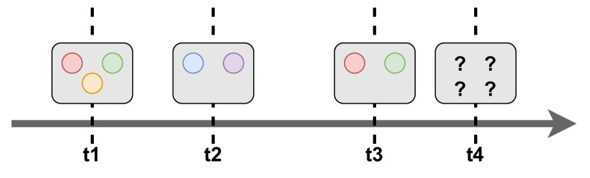
Figure 1: A dataset sample of timestamped events that can be used within the multi-label classification task and its visualization. ID refers to a considered client identifier, while features are additional characteristics of labels in a set. For example, if a set of labels are a group of transactions, then features represent the amounts of particular transactions. Our model should predict labels for the $28$th of August, given the history of previous label sets. There are multiple labels to predict, so it is a multi-label classification problem. The right figure provides a visual representation of the problem in the left table.

The interaction between an object’s states at different timestamps is essential for solving tasks with sequential data [10]. Therefore, expressive and powerful models should be able to learn such interactions. Several neural network architectures, such as transformers or recurrent neural networks, are capable of doing this. For example, a transformer directly defines an attention mechanism that measures how different timestamps in a sequence are connected. However, the applications of modern deep learning methods are limited [43], and they primarily focus on predicting labels for a sequence in general. We refer to the graph of connections between states of an object at different timestamps as a timestamp interaction graph.

Another connection worth exploring is the connection between different labels and a need to consider the correlation between them [9]. This capability is not inherent for the majority of models. With a large number of possible labels, this problem becomes close to a recommender system problem. We name the graph of connections between different labels a label interaction graph.

For single label-event data by using a position encoder, we take into account both interaction between labels and timestamped events [16, 40]. For sequential multi-label prediction, simultaneous consideration of both timestamp interaction graph and label interaction graph can be crucial. Typically, articles explore a particular side of the dependence that can be explainable by domain bias. In sequential recommender systems, there is a focus on connections between labels [23] with the incorporation of convolutional neural networks [28] as well as the attention mechanism [42]. Direct models for event sequences [11] also prefer identification of interactions between timestamps [44]. So, in time series and natural language processing, it is more common to handle a timestamp interaction graph via an attention mechanism or recurrent neural networks.

	LSTM	TransformerBase	CLASS2C2AE	LANET (ours)
Micro-AUC	2	3.2	3.6	1.2
Macro-AUC	2	3.2	3.6	1.2
Micro-F1	1.8	3.4	3.4	1.6
Macro-F1	1.8	3.2	2.8	2.2

Table 1: Mean rank for different metrics averaged over $5$ considered datasets. We want to minimize rank, as the best method has rank $1$. The best values are in bold and the second best values are underlined.

Our LANET aims at recovering label interaction graphs, as we believe it is more vital in many problems. The algorithm aggregates past information in a specially constructed set of label representations. The set serves as input to a transformer encoder. The transformer encoder updates label embeddings via self-attention, uncovering their interactions. Finally, we predict a set of labels for the current model based on the model’s output that encompasses knowledge of label relationships. Moreover, we can process long sequences this way, as now the attention evaluation is quadratic in the number of labels, not the sequence length. As our model does not use external information, it produces self-supervised embeddings.

Contributions.

We have developed a transformer-based architecture with self-attention between labels to deal with multi-label classification for event sequences. Our main contributions are the following:

• We introduce LANET architecture for the prediction of a label set for the current event taking the information from previous events. The architecture’s peculiarity is a calculation of self-attention between label views. The scheme of our approach is presented in Figure 2.

• LANET outperforms transformer-based models that focus on self-attention between timestamps. We evaluate all metrics on various datasets to prove the insufficiency of a common sequential placement-oriented perspective. See Table 1 for a high-level comparison of different approaches. Furthermore, we provide an ablation study of the proposed architecture.

• Due to LANET structure, it efficiently captures label interactions via the attention matrix.

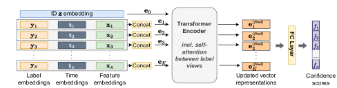
Figure 2: LANET architecture for multi-label classification of event sequences with a total number of labels $K$. The model input comprises the concatenation of the object’s label, time, feature, and ID embeddings. After self-attention layers, the model outputs a vector of confidence scores, where each element is associated with the probability of the presence of a particular label in the next event. The self-attention layer in LANET acts between labels, not temporal representations.

2 Related Work

The multi-label classification problem statement emerges in many diverse domains, e.g., text categorization or image tagging, all of which entail their own peculiarities and challenges. The review [41] explores foundations in multi-label learning, discussing the well-established methods as well as the most recent approaches. Emerging trends are covered in a more recent review [19].

Firstly, we examine loss functions tailored for the multi-label setting and into some methods for composing label set prediction. Secondly, we overview the usage of RNNs in the multi-label classification task. Thirdly, we review how to capture the label dependencies. Then, we discuss an association with a sequential recommendation problem. Lastly, we summarise the literature analysis and present the identified research gap.

Loss functions and ways for label set composition in multi-label problem.

The paper [21] studies the theoretical background for main approaches to the reduction of multi-label classification problem to a series of binary or multi-class problems. In particular, they show that considered reductions implicitly optimize for either Precision@k or Recall@k. The choice of the correct reduction should be based on the ultimate performance measure of interest. In [17], the authors propose an improved loss function for pairwise ranking in multi-label image classification task that is easier to optimize. Also, they discuss an approach based on the estimation of the optimal confidence thresholds for the label decision part of the model that determines which labels to include in the final prediction. The task of multi-label text classification is the topic of [5]. The authors construct an end-to-end deep learning framework called ML-Net. ML-Net consists of two parts: a label prediction network and a label count prediction network. In order to get the final set of labels, confidence scores generated from the label prediction network are ranked, and then the top $K_{top}$ labels are predicted. A separate label count network predicts $K_{top}$.

Neural networks for multi-label classification.

In [38], the authors use the RNN model to solve a multi-label classification problem. They address the issue that RNNs produce sequential outputs, so the target labels should be ordered. The authors propose to dynamically order the ground truth labels based on the model predictions, which contributes to faster training and alleviates the effect of duplicate generation. In turn, [31] consider the transformation of a multi-label classification problem to a sequence prediction problem with an RNN decoder. They propose a new learning algorithm for RNN-based decoders which does not rely on a predefined label order. Consequently, the model explores diverse label combinations, alleviating the exposure bias. The work [26] examines the same problem statement of multi-label classification in an event stream as we do. The authors’ model targets capturing temporal and probabilistic dependencies between concurrent event types by encoding historical information with a transformer and then leveraging a conditional mixture of Bernoulli experts.

Approaches to leveraging label dependencies.

The authors of [15] construct a model called C-Tran for a multi-label image classification task that leverages Transformer architecture that encourages capturing the dependencies among image features and target labels. The key idea is to train the model with label masking. The authors in [39] propose DNN architecture for solving the multi-label classification task, which incorporates the construction of label embeddings with feature and label interdependency awareness. A label-correlation sensitive loss improves the efficiency of the constructed model. Another popular way to consider label relationships is to use Graph Neural Networks as a part of the pipeline. Namely, [22] captures the correlation between the labels in the task of Multi-Label Text Classification by adopting Graph Attention Network (GAT). They predict the final set of labels combining feature vectors from BiLSTM and attended label features from GAT. Event sequences processing also tries to derive dependencies between different event types and consider specific attention mechanisms [20]. The closest to our LANET approach [18] in the literature explores the relationship between different series for multivariate time series classification. The authors propose using attention in step-wise and channel-wise fashion to produce embeddings, which are then forwarded by a classification head.

Sequential recommender systems.

Another close neighbour of our problem statement is the problem of sequential recommender system construction [34, 23]. In this case, we have a lot of possible labels and should sort them with respect to the probability of occurrence next time. Typically, the estimation of embeddings for all possible labels/items is a part of a pipeline. Existing approaches use neural networks for sequential data such as LSTM [35] as well as attention mechanism [33]. We want to highlight the statement related to the usage of only recent past data for prediction [16]. However, millions of possible labels typically lead to more classic techniques in this area with specific loss functions and methods.

Research gap.

Almost all existing methods are applied to multi-label learning for images, natural language texts or time series. However, there is a need for approaches to the multi-label classification of event sequences. Such characteristics of events as time-dependency and heterogeneous attributes introduce additional difficulties as well as opportunities for their processing and learning of label correlations. Notably, such data structure encourages the usage of the attention mechanism, as the sets of possible labels in the past and the future coincide, and it is natural to leverage such a connection in an architecture.

3 Methods

3.1 Multi-label sequential classification

We consider a multi-label classification for a sequence $S=\{(X_{i},Y_{i})\}_{i=1}^{t-1}$. It consists of a set of labels $Y_{i}$ and a set of features $X_{i}$ specific for each timestamp from $1$ to $t-1$. The index corresponds to the time of the event, so $(X_{1},Y_{1})$ is the information about the first event, and $(X_{t-1},Y_{t-1})$ is the information about the last observed event. A set $Y_{i}\subseteq\mathcal{Y}$, where $\mathcal{Y}=\{1,2,\dots,K\}$ is the set of all possible labels. A set size of $X_{i}$ is equal to a set size of $Y_{i}$. Each label from $Y_{i}$ is entailed with the numerical or categorical feature from $X_{i}$ in the corresponding position. We also can have an additional feature vector $\mathbf{z}$ describing a considered sequence $S$ as a whole, e.g. user ID. The goal of sequential multi-label classification is to predict a set of labels $Y_{t}$ for the next timestamp.

We construct a function $f(\cdot)\in[0,1]^{K}$ that takes the historical information on events as input and outputs the vector of scores for each of $K$ labels. Each score is an estimate of the probability of a label to be present in the next event-related label set. In our setting, we limit the size of the past available to our model. $S^{t}=\{(X_{j},Y_{j})\}_{j=t-\tau}^{t-1}$, where $\tau$ means a number of events preceding the considered event with the timestamp $t$, which is attributed with a target label set $Y_{t}$. So, more formally $f(\cdot)$ has the form:

$$f(X_{t-\tau},\ldots,X_{t-1},Y_{t-\tau},\ldots,Y_{t-1},\textbf{z})\in[0,1]^{K}$$

to prepare scores for the prediction of $Y_{t}$.

To complete a prediction, we need a separate label decision model $g(f(\cdot))$, that transforms confidence scores into labels. For example, we compare the score for $k$-th label to a selected threshold $\beta_{k}$: if $f_{k}(\cdot)>\beta_{k},k=1,\dots,K$, then the model predicts that the $k$-th label is present. Thus, the model $g$ produces a label set $\hat{Y}_{t}\subseteq\mathcal{Y}$ from the input confidence scores.

The resulting quality of the model depends both on the method $g(\cdot)$ for selecting labels to a final set and the performance of $f(\cdot)$ to produce confidence scores while we focus on working with $f(\cdot)$.

3.2 Dataset structure

We consider problems with the following dataset structure. See Figure 1 for an example of a data sample.

• ID. Each sequence that corresponds to a client or an organization has a unique identifier. So in our case, the feature vector for a sequence description is just a scalar value $z$. There may be thousands of unique IDs in the dataset. Nevertheless, we as well provide the results of experiments without the usage of ID information.

• Date. Each event is associated with a date.

• Labels. The label’s column provides a set of categorical variables $Y_{i}$ that describes an event. It might be a sequence of codes of transactions made by a client in a particular day or the categories of the sold items.

• Features. Each event is also characterized by a feature set $X_{i}$. It is represented as a set of categorical or numerical values. Each component in a set describes the corresponding label from a label set. Values of a feature set may have a meaning of the sums of paid money per transaction code or the number of the sold items per category.

3.3 Sample structure

We work within a sequential multi-label classification problem in the panel setting. The considered datasets have the structure $\mathcal{D}=\{(S_{j},z_{j})\}_{j=1}^{n}$. Each $S_{j}$ is a sequence of pairs of feature sets and corresponding multi-label sets. We need to split sequences $S_{j},j=1,\dots,n$ into samples for model training and testing. The part of a sample that is passed to the model’s input $f(\cdot)$ incorporates information on $\tau$ consecutive events from $S_{j}$ preceding the considered timestamp $t$. The sample’s target is a label set of the event from $S_{j}$ with the considered timestamp $t$. Thus, to construct train and test samples from the initial sequence $S_{j}$, we need to apply a sliding window approach. Importantly, train and test datasets that share the samples related to the same $z_{j},j=1,\dots,n$ organized in a non-overlapping and chronological way.

3.4 Our LANET approach

Most of the transformer-related models used for sequential multi-label prediction use self-attention computation between consecutive input timestamps representations. The LANET instead uses the self-attention between label representations. So, it has the input that consists of $K$ vectors. Below, we describe how to aggregate a sequence of size $\tau$ to $K$ vectors via an Embedding layer. Then we define the Self-attention layer. To get the predictions, we apply a Prediction layer.

Embedding layer.

We use the following approach to use different parts of input data for multi-label event sequences:

• ID embedding: For IDs we learn an embedding matrix;

• Time embedding: For each timestamp, we know the value of $dt$, which is equal to the difference in days between the considered and the previous timestamp. We train an embedding for each observed $dt$ value. We also take into account the order of events, so we look at the embeddings for positions: $1,\dots,$ $\tau$ to add them to the $dt$ representation of the corresponding timestamp;

• Amount embedding: We transform all amounts into bins, breaking down the continuous sums of amounts on the interval. Each interval is assigned a unique number. Then, for each unique number, we create embedding. A vector of representations is learned similar to [8].

• Transformer label encoder: To construct the LANET’s input, we use the data associated with a specific ID for $\tau$ timestamps. We concatenate the representation of the labels that are encountered during $\tau$ timestamps with the corresponding time and amount embeddings. If a label does not belong to a history of $\tau$ last timestamps, we add vectors of zeros to it as time and amount views. If a particular label occurs several times during previous $\tau$ steps, then we construct time embeddings for each individual occurrence and then sum them up to get the ultimate time view for that label. We do the same when constructing amount embedding in the situation of label reoccurrence.

So, as a result of the embedding layer, we have $K+1$ embedding vectors. The first vector $\mathbf{e}_{0}$ corresponds to the embeddings of general (ID) features for a sequence. All other vectors $\mathbf{e}_{k},k=1,\dots,K$ are concatenation of the label embedding with the corresponding time and amount embeddings. It turns out that vectors for not historically involved labels are just label embeddings, as we are summing them up with zero vectors of time and and amount views. Under the training of all embedding weights, they are initialized from normal distribution $\mathcal{N}(0,1)$ and then optimized.

Self-attention layer.

After getting representations from our data, we move on to the composition of our architecture. Let $E=\{\mathbf{e}_{0},\dots,\mathbf{e}_{K}\}$, $\mathbf{e}_{i}\in\mathbb{R}^{d}$, be the sequence of input embeddings to the Transformer encoder, where $\mathbf{e}_{0}$ corresponds to the embedding of $\mathbf{z}$ and all other $\mathbf{e}_{i}$ correspond to embeddings captured historical information from a label point of view. In Transformer architecture, the influence of embedding $\mathbf{e}_{j}$ on embedding $\mathbf{e}_{i}$ is obtained via self-attention. The attention weight $\alpha_{ij}$ and an embedding update $\mathbf{e}_{i}^{\prime}$ are calculated as:

$$\mathbf{e}_{i}^{\prime}=\sum_{j=0}^{K}\alpha_{ij}(W^{v}\mathbf{e}_{j});\hskip 8.53581pt\alpha_{ij}=\mathrm{softmax}\left((W^{q}\mathbf{e}_{i})^{T}(W^{k}\mathbf{e}_{j})/\sqrt{d}\right),$$

where $W^{k}$ is the key weight matrix, $W^{q}$ is the query weight matrix, and $W^{v}$ is the value weight matrix. Such a procedure of embedding updates can be repeated several times by specifying the number of Transformer encoder layers.

Prediction layer.

The updated embeddings are processed with one fully-connected linear layer to get final embeddings for each label $\{\mathbf{e}^{(final)}_{j}\}_{j=1}^{K}$. In this way, we obtain $\{f_{j}\}_{j=1}^{K}$ that are used in a multi-label classifier with threshold $t_{j}$ selected separately for each label using a validation sample.

4 Experiments

In this section, we present comparison of our approach with others and relevant ablation studies. The code is available at GitHub repository.

4.1 Datasets

	Dataset	# events	Median	Max	# unique	Diff
			set size	set size	labels
	Sales	47 217	16	48	84	0.0632
	Demand	5 912	13	24	33	0.0957
	Liquor	291 029	14	66	107	0.0413
	Transactions	784 520	3	23	77	0.1079
	Orders	226 522	2	13	61	0.0518

Table 2: Characteristics of the datasets used in sequential multi-label classification problems.

For a more versatile study of the algorithm we built, we conducted experiments on five diverse datasets. Sales dataset [4] is historical sales data from different shops. The labels relate to the item categories, and the amount is the number of sold items for a particular category. Demand dataset [7] describes historical product demand of several warehouses. The label feature means the product category, and the amount feature relates to the corresponding demand. Liquor dataset [27] presents information on the liquor sales of the different stores. Each liquor label is identified by its category. The amount of sold liquor is measured in litres. Transactions dataset [2] contains histories of clients transactions. Each transaction is described with the special MCC code and an involved amount of money. In the original paper, the dataset has the name Gender. To demonstrate the applicability of the proposed approach in the industry, we also consider a private Orders dataset. It provides information on the restaurant orders of different materials for beer production. The amount feature is related to the volume of ordered materials in hectolitres.

The overall statistics for the considered datasets are given in Table 2. We present the number of observed events, Median set size of all available label sets $\mathrm{median}({|Y_{ij}|}_{i,j=1,1}^{n,t_{i}})$, Maximum size of the label set that is encountered in the dataset $\max({|Y_{ij}|}_{i,j=1,1}^{n,t_{i}})$, the number of unique labels $K$, and Diff. Diff measures the imbalance of labels: we calculate 5$\%$ and 95$\%$ quantiles for frequencies of labels and take the difference between them. The representation of labels is imbalanced in the majority of datasets, but we use metrics that take into account this effect. All datasets are transformed to a general structure described in Figure 1.

Dataset	Model	Micro-AUC$\uparrow$	Macro-AUC$\uparrow$	Micro-F1$\uparrow$	Macro-F1$\uparrow$
	LSTM	0.8670	0.7346	0.5600	0.4389
	TransformerBase	0.8604	0.7206	0.5348	0.3751
	CLASS2C2AE	0.8528	0.6881	0.5116	0.4217
Sales	LANET (ours)	0.9069	0.7627	0.6235	0.4901
	LSTM	0.8829	0.7633	0.6746	0.5929
	TransformerBase	0.8624	0.7240	0.6491	0.5678
	CLASS2C2AE	0.8342	0.7079	0.6738	0.5581
Demand	LANET (ours)	0.8806	0.7373	0.7038	0.5908
	LSTM	0.7520	0.7253	0.4729	0.2218
	TransformerBase	0.7501	0.7197	0.4674	0.2279
	CLASS2C2AE	0.9442	0.8058	0.4088	0.3638
Liquor	LANET (ours)	0.9536	0.8728	0.7089	0.4508
	LSTM	0.9719	0.8189	0.2133	0.2349
	TransformerBase	0.9714	0.8098	0.1982	0.2285
	CLASS2C2AE	0.9347	0.7324	0.1131	0.1501
Transactions	LANET (ours)	0.9743	0.8328	0.2373	0.1067
	LSTM	0.9800	0.9562	0.6827	0.6280
	TransformerBase	0.9601	0.9316	0.6302	0.5631
	CLASS2C2AE	0.9218	0.8964	0.6324	0.5979
Orders	LANET (ours)	0.9847	0.9665	0.5773	0.5856

Table 3: Comparison of our method LANET with the baselines on five different datasets. Best values are highlighted, and second-best values are underlined.

4.2 Baselines and training details

TransformerBase utilizes the transformer architecture [32]. Similar to many previous works, it considers the self-attention between input vectors that correspond to consecutive points in a sequence. We also note that it can be viewed as a simplification of next-item-recommendation models [16]. The amount vector for each timestamp is the input vector, whose dimension is equal to the number of the unique label values. Each position of the vector contains the corresponding amount value. There is no need for label embedding, as the information on historically involved labels is introduced through the amount vector. Time and ID embeddings are constructed in the same way as in LANET. We also use two self-attention layers. The output of the transformer encoder is an updated time representation. Subsequently, Mean Pooling is applied to this output to obtain the final vector of confidence estimates, based on which we make a prediction on a set of labels for the current timestamp.

We also use two RNN-based approaches. RNN (LSTM) replaces the transformer encoder with LSTM-type encoder [13]. The model takes one by one point in time and updates the hidden representation, which contains information about previous elements. CLASS2C2AE is a model for multilabel-classification presented in [39]. This model combines LSTM and autoencoder to improve its performance.

For all models, we use the same data input given in Subsection 3.2. The following manually selected hyperparameters were used for all experiments: dimension of the embedding space is 128, batch size is 32. We use Adam optimizer with learning rate initialized to $0.001$ and reduced via reduce-LR-on-plateau scheduler.

LANET training details.

Our LANET model consists of two Transformer encoder layers with four heads in each layer. Self-attention and layer implementation are inherited from the basic PyTorch Transformer layer [1]. After receiving the updated vector representations, we run them through the dropout layer, which is initialized with the probability $0.3$. In the end, a fully-connected linear layer is applied to the obtained vectors to get final label scores. LANET is trained with the cross-entropy loss adapted for the multi-label task through independent consideration of each label score.

Validation procedure.

The original datasets are divided into train, validation, and test sets. For each ID, some part of the consecutive events go to the train set, and the rest is allocated for validation and test. Importantly, the time periods in the train, valid, and test sets do not overlap and are arranged in the order of increasing time. We take 70% of the data samples for model training, 17% for validation, and 13% for testing. All experiments were also carried out for five random seeds, and the results after the experiments were averaged.

The article [36] provides an overview of metrics for multi-label classification. We consider the most frequently used and comprehensive metrics for the estimation of multi-label classification quality: Micro-AUC, Macro-AUC, Micro-F1, and Macro-F1.

4.3 Main results

For all datasets, the models are trained with five different random seeds to understand the value of results deviation from the result depending on the selected random state. The standard deviation influences the metrics in the third decimal place, while the superiority in performance is observed in the first or second decimal place. To make our tables more readable, we omit the standard deviation values. To calculate micro-F1 and macro-F1, we search for thresholds to compare them with the obtained confidence scores and compose the final label set. Thresholds are selected on the validation set by optimizing F1-score for each label separately.

Table 3 presents the sequential multi-label classification metrics for considered approaches. Our LANET gives the best results for diverse datasets. The LSTM baseline is also suitable for capturing the label relationships in general. We denote that it gives better results than the used version of transformer. The reason can be the limited amount of data for training available, so there are too many parameters for a transformer with timestamp-based self-attention. Besides, we test the model suggested in [26] for our problems. However, the results were not satisfying. We associate it with a more complex structure and, consequently, greater sensitivity to model parameters.

4.4 Ablation study

In this section, we provide results of ablation studies. The results are for Demand dataset, if not mentioned otherwise, as for most of the other datasets conclusions are similar.

Usage of both label-attention and timestamp-attention.

It is worth exploring what perspective of self-attention calculation is more critical: between labels or between timestamps. Table 4 answers this question. Label-attention is our basic implementation. Time-attention is a case when we consider attention only between timestamp views. Concat-attention implies getting confidence scores from concatenation of label-attention and time-attention. We learn the importance coefficients of two forms of attentions and use them as weights when summing attention views in the case of gated-attention. Absence-indication experiment consists in adding a learnable vector to the input embeddings if the particular label is not involved in the considered history. As a result, Label-attention is the most beneficial, and the inclusion of both types of attention decreases the quality.

	Micro-AUC$\uparrow$	Macro-AUC$\uparrow$	Micro-F1$\uparrow$	Macro-F1$\uparrow$
Label-attention	0.881 $\pm$ 0.007	0.737 $\pm$ 0.017	0.704 $\pm$ 0.018	0.591 $\pm$ 0.003
Time-attention	0.837 $\pm$ 0.004	0.682 $\pm$ 0.007	0.674 $\pm$ 0.009	0.588 $\pm$ 0.002
Concat-attention	0.835 $\pm$ 0.001	0.681 $\pm$ 0.010	0.666 $\pm$ 0.000	0.587 $\pm$ 0.001
Gated-attention	0.829 $\pm$ 0.030	0.668 $\pm$ 0.048	0.672 $\pm$ 0.010	0.578 $\pm$ 0.011
Absence-indication	0.882 $\pm$ 0.004	0.742 $\pm$ 0.003	0.704 $\pm$ 0.010	0.589 $\pm$ 0.004

Table 4: Comparison of metrics when calculating attentions between different views in LANET.

The contribution of different feature embeddings to model performance.

The input to our LANET model consists of a label, time, amount, and ID that we embed to input to the self-attention layer. All these parts include information on the events preceding the considered one. We want to understand the contribution of each feature embedding to the model prediction. So, in each experiment, we drop either amount, time, and ID one at a time. A significant quality drop after removal indicates the importance of the model part for the prediction. The results of such an experiment are in Table 5.

Inputs	Micro-AUC$\uparrow$	Macro-AUC$\uparrow$	Micro-F1$\uparrow$	Macro-F1$\uparrow$
All	0.881 $\pm$ 0.007	0.737 $\pm$ 0.017	0.704 $\pm$ 0.018	0.591 $\pm$ 0.003
No amount	0.825 $\pm$ 0.051	0.705 $\pm$ 0.039	0.698 $\pm$ 0.010	0.574 $\pm$ 0.014
No time	0.869 $\pm$ 0.007	0.721 $\pm$ 0.020	0.698 $\pm$ 0.004	0.590 $\pm$ 0.003
No ID	0.880 $\pm$ 0.003	0.732 $\pm$ 0.006	0.703 $\pm$ 0.022	0.588 $\pm$ 0.004

Table 5: How different types of embeddings in the architecture affect LANET.

A substantial drop in quality happens when we drop the amount embeddings. We attribute this effect to the fact that amounts are essential for quantifying the scale of interdependencies. Time embeddings are helpful and make models capture label connections better. IDs contribute little to the performance of the model. It seems that it is enough to look at other types of available information.

Dependence of model quality on $\tau$.

The model considers only $\tau$ last timestamps for prediction. Thus, a natural question arises about how the model quality depends on the number of timestamps used for prediction. The dependence of micro-AUC metric on $\tau$ is presented in 3(a).

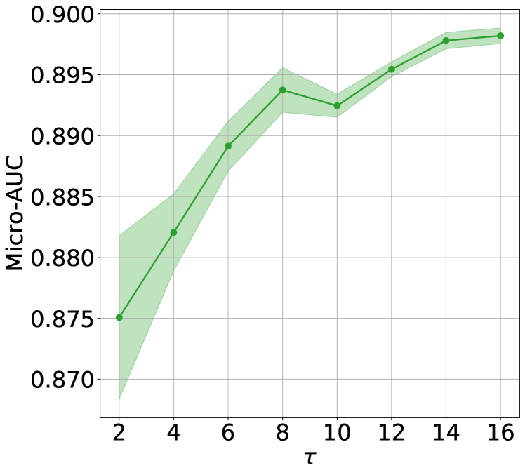
(a) The dependence of micro-AUC on the $\tau$ parameter.

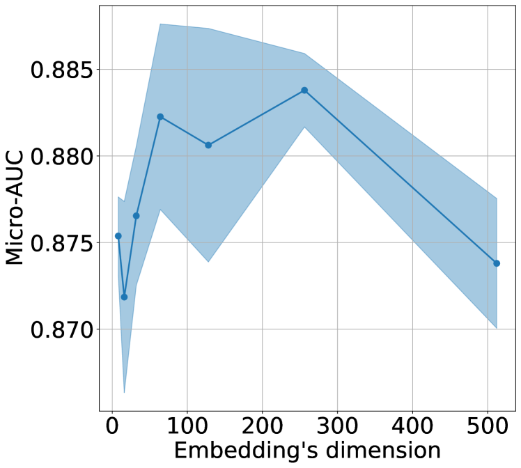
(b) The dependence of micro-AUC on the dimension of embeddings.

Figure 3: The dependence of metrics on model parameters for Demand dataset.

The experiment supports the evidence that the more information we provide to our model, the better prediction we obtain for the considered timestamp. However, we should find the balance between the desired quality and the computational cost since the number of involved labels increases with boosting parameter value. Therefore, for the optimality of the solution and the speed of the method, we selected the parameter $\tau=3$.

Dependence of the model performance on embedding size.

As we are working with learnable embeddings for label, amount, time, and ID features, we need to set the dimensionality of their representations. For each feature, we construct embeddings of the same size. The dimensionality of the embedding vector defines the capacity of information that a model should capture and the overall number of learnable parameters. The results are in 3(b). We can observe that the model can not effectively learn large-dimension representations.

Attention matrix for vector representations of labels

Additionally, we constructed an attention matrix for the data labels. This matrix reflects label importances for making predictions. The model pays attention to various sequence objects with different weights. Figure 4 shows three attention matrices for three datasets: Order, Transactions, and Liquor. The size of the matrix is the number of unique labels in the dataset. We notice that the attention matrix has a clear dominance of the certain labels encountered in the sequence over those that are not in it, which is clearly expressed through the weights. Looking deeper, we see that small-scale variations in attention describe the connection between particular event types.

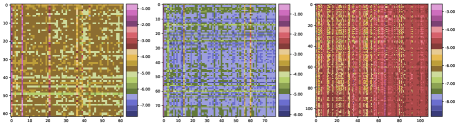
Figure 4: Attention matrix studies for the Orders, Transactions and Liquor datasets from left to right. They show the representation importances.

5 Conclusions and discussion

We consider the sequential multi-label classification problem: given previous multi-label vectors, what a multi-label vector will be next. For this problem, we propose the LANET architecture. It explores a connection between past multi-label vectors in a specific architecture. In particular, LANET uses the self-attention between labels to encourage capturing historical label interdependencies. In our pipeline, we can apply any model architecture based on any similar self-attention. So, it can easily absorb attention-related innovations making it possible to add interpretability [24] or efficiency [30] to a model.

LANET demonstrates the best metrics on the five considered datasets. In particular, it improves the micro-AUC metric from $0.7501$ to $0.9536$ on one of the datasets. However, the current approach is limited to the case where no long-term memory is required for prediction, as we aggregate only several recent timestamps and general embeddings of a particular sequence. Further studies are welcomed to fill this gap.

It is also interesting to note that the proposed approach naturally fits into the paradigm of self-supervised learning and directly outputs an embedding of a client in general and at a particular time. The intricacy of the self-supervised problem is easy to tune by changing the used time horizon or including masking during training [12, 14]. By aggregating labels collected during a day, we also make learning event sequences models more stable, avoiding the over-complicated problem of predicting the next event type [3] and challenging likelihood optimization for neural temporal points processes [25].

References

- [1] https://pytorch.org/docs/stable/generated/torch.nn.TransformerEncoderLayer.html
- [2] Prediction of client gender on card transactions. https://www.kaggle.com/c/python-and-analyze-data-final-project/data (2019)
- [3] Babaev, D., Ovsov, N., Kireev, I., Ivanova, M., Gusev, G., Nazarov, I., Tuzhilin, A.: Coles: Contrastive learning for event sequences with self-supervision. In: Proceedings of the 2022 International Conference on Management of Data. pp. 1190–1199 (2022)
- [4] Company, C.: Predict Future Sales. https://www.kaggle.com/c/competitive-data-science-predict-future-sales/data (2018)
- [5] Du, J., Chen, Q., Peng, Y., Xiang, Y., Tao, C., Lu, Z.: Ml-net: multi-label classification of biomedical texts with deep neural networks. Journal of the American Medical Informatics Association 26(11), 1279–1285 (2019)
- [6] Durand, T., Mehrasa, N., Mori, G.: Learning a deep convnet for multi-label classification with partial labels. In: Proceedings of the IEEE/CVF Conference on Computer Vision and Pattern Recognition. pp. 647–657 (2019)
- [7] FELIXZHAO: Forecasts for Product Demand. https://www.kaggle.com/datasets/felixzhao/productdemandforecasting (2017)
- [8] Fursov, I., Morozov, M., Kaploukhaya, N., Kovtun, E., Rivera-Castro, R., Gusev, G., Babaev, D., Kireev, I., Zaytsev, A., Burnaev, E.: Adversarial attacks on deep models for financial transaction records. In: Proceedings of the 27th ACM SIGKDD Conference on Knowledge Discovery & Data Mining. pp. 2868–2878 (2021)
- [9] Hang, J.Y., Zhang, M.L.: Collaborative learning of label semantics and deep label-specific features for multi-label classification. IEEE Transactions on Pattern Analysis and Machine Intelligence (2021)
- [10] Hartvigsen, T., Sen, C., Kong, X., Rundensteiner, E.: Recurrent halting chain for early multi-label classification. In: Proceedings of the 26th ACM SIGKDD International Conference on Knowledge Discovery & Data Mining. pp. 1382–1392 (2020)
- [11] Hawkes, A.G.: Spectra of some self-exciting and mutually exciting point processes. Biometrika 58(1), 83–90 (1971)
- [12] He, K., Chen, X., Xie, S., Li, Y., Dollár, P., Girshick, R.: Masked autoencoders are scalable vision learners. In: Proceedings of the IEEE/CVF Conference on Computer Vision and Pattern Recognition. pp. 16000–16009 (2022)
- [13] Hochreiter, S., Schmidhuber, J.: Long short-term memory. Neural computation 9(8), 1735–1780 (1997)
- [14] Kenton, J.D.M.W.C., Toutanova, L.K.: Bert: Pre-training of deep bidirectional transformers for language understanding. In: Proceedings of NAACL-HLT. pp. 4171–4186 (2019)
- [15] Lanchantin, J., Wang, T., Ordonez, V., Qi, Y.: General multi-label image classification with transformers. In: Proceedings of the IEEE/CVF Conference on Computer Vision and Pattern Recognition (CVPR). pp. 16478–16488 (June 2021)
- [16] Li, J., Wang, Y., McAuley, J.: Time interval aware self-attention for sequential recommendation. In: Proceedings of the 13th international conference on web search and data mining. pp. 322–330 (2020)
- [17] Li, Y., Song, Y., Luo, J.: Improving pairwise ranking for multi-label image classification. In: Proceedings of the IEEE Conference on Computer Vision and Pattern Recognition (CVPR) (July 2017)
- [18] Liu, M., Ren, S., Ma, S., Jiao, J., Chen, Y., Wang, Z., Song, W.: Gated transformer networks for multivariate time series classification. arXiv preprint arXiv:2103.14438 (2021)
- [19] Liu, W., Wang, H., Shen, X., Tsang, I.: The emerging trends of multi-label learning. IEEE transactions on pattern analysis and machine intelligence (2021)
- [20] Mei, H., Yang, C., Eisner, J.: Transformer embeddings of irregularly spaced events and their participants. In: International Conference on Learning Representations (2021)
- [21] Menon, A.K., Rawat, A.S., Reddi, S., Kumar, S.: Multilabel reductions: what is my loss optimising? Advances in Neural Information Processing Systems 32 (2019)
- [22] Pal, A., Selvakumar, M., Sankarasubbu, M.: Multi-label text classification using attention-based graph neural network. arXiv preprint arXiv:2003.11644 (2020)
- [23] Quadrana, M., Cremonesi, P., Jannach, D.: Sequence-aware recommender systems. ACM Computing Surveys (CSUR) 51(4), 1–36 (2018)
- [24] Serrano, S., Smith, N.A.: Is attention interpretable? In: Proceedings of the 57th Annual Meeting of the Association for Computational Linguistics. pp. 2931–2951 (2019)
- [25] Shchur, O., Türkmen, A.C., Januschowski, T., Günnemann, S.: Neural temporal point processes: A review. arXiv preprint arXiv:2104.03528 (2021)
- [26] Shou, X., Gao, T., Subramaniam, S., Bhattacharjya, D., Bennett, K.: Concurrent multi-label prediction in event streams. In: AAAI Conference on Artificial Intelligence (2023)
- [27] T, B.: Time Series Analysis of Iowa Liquor Sales. https://www.kaggle.com/code/roudradas/time-series-analysis-of-iowa-liquor-sales/data (2020)
- [28] Tang, J., Wang, K.: Personalized top-n sequential recommendation via convolutional sequence embedding. In: Proceedings of the eleventh ACM international conference on web search and data mining. pp. 565–573 (2018)
- [29] Tarekegn, A.N., Giacobini, M., Michalak, K.: A review of methods for imbalanced multi-label classification. Pattern Recognition 118, 107965 (2021)
- [30] Tay, Y., Dehghani, M., Bahri, D., Metzler, D.: Efficient transformers: A survey. ACM Computing Surveys 55(6), 1–28 (2022)
- [31] Tsai, C.P., Lee, H.Y.: Order-free learning alleviating exposure bias in multi-label classification. In: Proceedings of the AAAI Conference on Artificial Intelligence. vol. 34, pp. 6038–6045 (2020)
- [32] Vaswani, A., Shazeer, N., Parmar, N., Uszkoreit, J., Jones, L., Gomez, A.N., Kaiser, Ł., Polosukhin, I.: Attention is all you need. Advances in neural information processing systems 30 (2017)
- [33] Wang, S., Hu, L., Cao, L.: Perceiving the next choice with comprehensive transaction embeddings for online recommendation. In: Machine Learning and Knowledge Discovery in Databases: European Conference, ECML PKDD 2017, Skopje, Macedonia, September 18–22, 2017, Proceedings, Part II 17. pp. 285–302. Springer (2017)
- [34] Wang, S., Hu, L., Wang, Y., Cao, L., Sheng, Q.Z., Orgun, M.: Sequential recommender systems: challenges, progress and prospects. In: 28th International Joint Conference on Artificial Intelligence, IJCAI 2019. pp. 6332–6338. International Joint Conferences on Artificial Intelligence (2019)
- [35] Wu, C.Y., Ahmed, A., Beutel, A., Smola, A.J., Jing, H.: Recurrent recommender networks. In: Proceedings of the tenth ACM international conference on web search and data mining. pp. 495–503 (2017)
- [36] Wu, X.Z., Zhou, Z.H.: A unified view of multi-label performance measures. In: International Conference on Machine Learning. pp. 3780–3788. PMLR (2017)
- [37] Xiao, L., Huang, X., Chen, B., Jing, L.: Label-specific document representation for multi-label text classification. In: Proceedings of the 2019 conference on empirical methods in natural language processing and the 9th international joint conference on natural language processing (EMNLP-IJCNLP). pp. 466–475 (2019)
- [38] Yazici, V.O., Gonzalez-Garcia, A., Ramisa, A., Twardowski, B., Weijer, J.v.d.: Orderless recurrent models for multi-label classification. In: Proceedings of the IEEE/CVF Conference on Computer Vision and Pattern Recognition. pp. 13440–13449 (2020)
- [39] Yeh, C.K., Wu, W.C., Ko, W.J., Wang, Y.C.F.: Learning deep latent space for multi-label classification. In: Thirty-first AAAI conference on artificial intelligence (2017)
- [40] Ying, H., Zhuang, F., Zhang, F., Liu, Y., Xu, G., Xie, X., Xiong, H., Wu, J.: Sequential recommender system based on hierarchical attention network. In: IJCAI International Joint Conference on Artificial Intelligence (2018)
- [41] Zhang, M.L., Zhou, Z.H.: A review on multi-label learning algorithms. IEEE transactions on knowledge and data engineering 26(8), 1819–1837 (2013)
- [42] Zhang, S., Tay, Y., Yao, L., Sun, A., An, J.: Next item recommendation with self-attentive metric learning. In: Thirty-Third AAAI Conference on Artificial Intelligence. vol. 9 (2019)
- [43] Zhang, W., Jha, D.K., Laftchiev, E., Nikovski, D.: Multi-label prediction in time series data using deep neural networks. arXiv preprint arXiv:2001.10098 (2020)
- [44] Zhuzhel, V., Grabar, V., Boeva, G., Zabolotnyi, A., Stepikin, A., Zholobov, V., Ivanova, M., Orlov, M., Kireev, I., Burnaev, E., Rivera-Castro, R., Zaytsev, A.: Continuous-time convolutions model of event sequences (2023)