Casimir effect, loop corrections and topological mass generation for interacting real and complex scalar fields in Minkowski spacetime with different conditions

Abstract

In this paper the Casimir energy density, loop corrections, and generation of topological mass are investigated for a system consisting of two interacting real and complex scalar fields. The interaction considered is the quartic interaction in the form of a product of the modulus square of the complex field and the square of the real field. In addition, it is also considered the self-interaction associated with each field. In this theory, the scalar field is constrained to always obey periodic condition while the complex field obeys in one case a quasiperiodic condition and in other case mixed boundary conditions. The Casimir energy density, loop corrections, and topological mass are evaluated analytically for the massive and massless scalar fields considered. An analysis of possible different stable vacuum states and the corresponding stability condition is also provided. In order to better understand our investigation, some graphs are also presented. The formalism we use here to perform such investigation is the effective potential, which is written as loop expansions via path integral in quantum field theory.

I Introduction

Since its prediction in 1948, the Casimir effect is considered one of the most interesting physical phenomenon. This effect, which is of pure quantum nature, was predicted by H. Casimir casimir1948attraction . In its standard form, the Casimir effect consists in a force of attraction that arises in a system of two neutral parallel and perfectly conducting plates, placed in a classical vacuum, near to each other. This force of attraction is described in the framework of quantum field theory and is due to modifications in the vacuum fluctuations associated with the quantized electromagnetic field, as a consequence of the imposition of Dirichlet boundary condition on the plates. The phenomenon of the Casimir effect, in the case of the electromagnetic field, has been confirmed by several high accuracy experiments bressi2002measurement ; kim2008anomalies ; lamoreaux1997demonstration ; lamoreaux1998erratum ; mohideen1998precision ; mostepanenko2000new ; wei2010results . Currently, it is also known that not only the electromagnetic field presents the Casimir effect, but other fields as well, such as scalar and fermion fields. Additionally, the Casimir effect may also arise from different boundary conditions. For instance, the Casimir effect associated with a real scalar field subjected to a helix boundary condition with temperature corrections is considered in Ref. aleixo2021thermal , subjected to Robin boundary conditions in Ref. romeo2002casimir , and in Ref. maluf2020casimir the Casimir energy for a real scalar field and the Elko neutral spinor field in a field theory at a Lifshitz fixed point is obtained. Moreover, in Ref. Haridev:2021jwi a complex scalar field theory has been considered and the corresponding Casimir energy density in compact spacetimes investigated. A review on the Casimir effect can be found in Ref. bordag2009advances (see also milton2001casimir ; mostepanenko1997casimir ).

As we have mentioned, boundary conditions play a crucial role in the investigation of the Casimir effect. A very interesting condition is the quasiperiodic one. In Ref. feng2014casimir a scalar field under a quasiperiodic condition, inspired by nanotubes, is considered in order to investigate the corresponding Casimir effect. It is found that the Casimir force can be attractive or repulsive depending on the value of the phase related to the quasiperiodic condition. Another interesting boundary condition that modifies the quantum vacuum fluctuations of a field is the one known as mixed boundary condition (Dirichlet - Neumann). The Casimir energy arising as a consequence of the imposition of mixed boundary conditions on a real self-interacting scalar field has been considered in Ref. barone2004radiative and in Ref. cruz2020casimir , where a Lorentz violation scenario is also taken into account. Also, in Ref. FariasJunior:2022qsp it is studied a scalar field with a quartic self-interaction restricted to obey a helix boundary condition.

The investigation of interacting quantum fields is important since fields found in nature are always interacting. The interaction mostly considered in the previous mentioned works is a quartic self-interaction. In the framework of two interacting quantum fields, using the effective potential approach, Toms in Ref. toms1980interacting have considered two real scalar fields, one twisted and the other untwisted, interacting via the so called quartic interaction, i.e., the product between the square of the two fields in a Euclidean spacetime, in order to investigate the symmetry breaking and mass generation as a consequence of the nontrivial topology produced by the periodic and antiperiodic conditions used. The quartic interaction between two real fields is also considered in Ref. wang2022particle for the study of the phenomenon of particle production from oscillating scalar backgrounds in a Friedmann-Lemaître-Robertson-Walker universe using non-equilibrium quantum field theory. In this type of calculation the renormalization procedure is of particular importance. In this sense, Ref. wysozka2021two presents a detailed discussion about the renormalization scheme present in quantum field theory comprising two interacting scalar fields.

In order to investigate the Casimir energy density, loop corrections and generation of topological mass, in the present paper, we consider a system consisting of two real and complex scalar fields interacting with each other via quartic interaction, in addition to the self-interactions which are normally present. The real field is always subject to a periodic condition while the complex field is restricted to obey a quasiperiodic condition, as well as mixed boundary conditions used on two identical and perfectly reflecting parallel planes separated by a distance $L$. Hence, we shall analyze separately two scenarios, one where a periodic real scalar field interacts with a complex scalar field obeying a quasiperiodic condition and the other where a periodic real scalar field interacts with a complex scalar field obeying mixed boundary conditions. These two scenarios generalize previous results found in the literature where it has been considered self-interacting real scalar fields under periodic toms1980symmetry ; Ford:1978ku and quasiperiodic porfirio2021ground conditions, and also under mixed boundary conditions barone2004radiative ; cruz2020casimir . In this regard, we extend the analysis performed in Ref. toms1980interacting to the complex scalar field and considering other conditions.

The choice of boundary conditions have to be mathematically consistent and the choice of mixed boundary conditions are natural, for instance, in the case of quantum gravity, spinor field theory and supergravity luckock1991mixed . Furthermore, the quasiperiodic condition plays an important role when one considers nanotubes or nanoloops for a quantum field feng2014casimir . For example, if the phase angle is zero (the periodic case), we have a corresponding system describing metallic nanotubes, while the values $\pm\frac{2\pi}{3}$ for the phase angle correspond to semiconductor nanotubes. In our investigation, we shall use the path integral formalism and construct the effective potential in terms of loop expansions. This formalism was developed by Jackiw jackiw1974functional and allows us to obtain the Casimir energy density and loop corrections. The formalism also allows us, in principle, to calculate loop corrections to the mass of the fields as a consequence of the nontrivial topology of the spacetime. In our case, we consider only one-loop correction to the mass, which is enough to see generation of topological mass at first order.

This paper is organized as follows: in Sec.II we review the main aspects of the path integral formalism to obtain the effective potential in the case of two interacting quantum fields, one real and the other complex. The interaction considered is the quartic interaction, that is, a product between the modulus square of the complex field and the square of the real field. In addition, we also consider self-interaction contributions for each field. In Sec.III, we consider the real and complex fields interacting with each other, where the real scalar field is subjected to a periodic condition, while the components of the complex field obey a quasiperiodic condition. By using the Riemann zeta function technique, we evaluate the effective potential of the system, the Casimir energy density and the one-loop correction to the mass. It is also discussed the conditions for the stability of the vacuum states, which leads to conditions for a positive topological mass. In Sec.IV the components of the complex field will now be subjected to mixed boundary conditions. The Casimir energy density, topological mass and the vacuum stability are also investigated. In Sec.V we present our conclusions. Through this paper we use natural units in which both the Planck constant and the speed of light are given by $\hslash=c=1$.

II Effective potential for interacting real and complex scalar fields

In this section we consider a real scalar field, $\psi$, interacting with a complex scalar one, that is, $\phi$. The interaction term is in the form of a product of the modulus square of the complex field and the square of $\psi$. This choice of interaction satisfies the discrete symmetry $\psi\rightarrow-\psi$, as well as the global symmetry $\phi\rightarrow e^{i\alpha}\phi$. The existence of symmetries in particle physics is crucial for the predicability of a given model and for a better fitting with experimental data Haber:2019iyb , making it important to consider this type of interactions in the investigation of the Casimir effect, for instance. Note that it is also considered the quartic self-interaction for each field. In the path integral approach for the evaluation of the effective potential, it is usual to work with the Euclidean spacetime coordinates, with imaginary time greiner2013field . Moreover, the complex field $\phi$ can be decomposed in terms of its real components as

$$\phi=\frac{1}{\sqrt{2}}\left(\varphi_{1}+i\varphi_{2}\right),\qquad\qquad\phi^{\ast}=\frac{1}{\sqrt{2}}\left(\varphi_{1}-i\varphi_{2}\right).$$

The model associated with the system described above, in Euclidean coordinates, is given by the following action:

$$S_{E}\left[\psi,\varphi_{i}\right]=\frac{1}{2}\int d^{4}x\left[\psi\square\psi+\sum_{i=1}^{2}\varphi_{i}\square\varphi_{i}\right]-\int d^{4}xU\left(\psi,\varphi\right),$$

$$U\left(\psi,\varphi\right)=\frac{m^{2}+C_{2}}{2}\psi^{2}+\frac{\mu^{2}}{2}\varphi^{2}+\frac{g}{2}\varphi^{2}\psi^{2}+\frac{\lambda_{\varphi}}{4!}\varphi^{4}+\frac{\lambda_{\psi}+C_{1}}{4!}\psi^{4}+C_{3},$$ (1)

where $m$ is the mass of the real field $\psi$, $\mu$ is the mass of the complex field $\phi$, $\lambda_{\psi}$ and $\lambda_{\phi}$ are the coupling constants of self-interaction for the real and complex fields, respectively, and $g$ is the coupling constant of the interaction between the fields. The parameters $C_{i}$’s are the renormalization constants and their explicit form will be obtained in the renormalization process of the effective potential for each case considered in the next sections. We also make use of the notation $\varphi^{2}=\varphi_{1}^{2}+\varphi_{2}^{2}$. Furthermore, the d’Alembertian operator, $\square$, is written in Euclidean spacetime coordinates as

$$\square=\left(\partial_{\tau}^{2}+\mathbf{\nabla}^{2}\right),$$ (2)

where $\tau=it$ is the imaginary time.

The construction of the effective potential using the path integral approach is described in detail in Refs. ryder1996quantum ; toms1980symmetry (see also cruz2020casimir ; porfirio2021ground ). Here we present only the main steps necessary to our purposes. Thus, the action in Eq. (1) is now expanded about a fixed background $\Psi$ and $\Phi_{i}$ that is, $\psi=\Psi+\chi$, $\varphi_{i}=\Phi_{i}+\varrho$, with $\chi$ and $\varrho$ representing quantum fluctuations. Since we are interested in the real field we seek to obtain the effective potential as a function only of $\Psi$, i.e., $V_{\mathrm{eff}}\left(\Psi\right)$. Then it is unnecessary to shift the components of the complex field $\phi$, which amounts to set $\Phi_{i}=0$ jackiw1974functional . Hence, we do not need to include counter terms proportional to powers of $\varphi$ in Eq. (1). A note here is in place, if we try to carry out the shift in $\phi$, i.e., setting $\Phi_{i}\neq 0$, a cross term will appear in the exponential on the r.h.s. of Eq. (5), which turns the calculations needed for the analysis extremely cumbersome. For this reason the simplification $\Phi_{i}=0$, is justified in the calculations. In the next sections we will in fact impose on the components of the complex field a quasiperiodic condition as well as mixed boundary conditions. This requires that we set the value $\Phi_{i}=0$, the only possible choice for a constant field to be compatible with the imposed conditions. In these cases, the use of Eq. (5) without cross terms becomes more accurate. Therefore, in the next sections, we shall be interested in analyzing the influence of the complex scalar field, subjected to a quasiperiodic and mixed conditions, on both the Casimir energy density and topological mass arising due to the real scalar field subjected to a periodic condition.

The expansion of the effective potential in powers of $\hslash$, up to order $\hslash^{2}$, can be written as

$$V_{\mathrm{eff}}\left(\Psi\right)=V^{\left(0\right)}\left(\Psi\right)+V^{\left(1\right)}\left(\Psi\right)+V^{\left(2\right)}\left(\Psi\right).$$ (3)

The zero order term, $V^{\left(0\right)}\left(\Psi\right)$, describes the classical potential, i.e., the tree-level contribution,

$$V^{\left(0\right)}\left(\Psi\right)=U\left(\Psi\right)=\frac{m^{2}+C_{2}}{2}\Psi^{2}+\frac{\lambda_{\psi}+C_{1}}{4!}\Psi^{4}+C_{3}.$$ (4)

The next term, $V^{\left(1\right)}\left(\Psi\right)$, is the one-loop correction to the classical potential and, in terms of the path integral approach, takes the following form toms1980interacting :

$$V^{\left(1\right)}\left(\Psi\right)=-\frac{1}{\Omega_{4}}\ln\int\mathcal{D}\psi\mathcal{D}\varphi_{1}\mathcal{D}\varphi_{2}\exp\left\{-\frac{1}{2}\left(\psi,\hat{A}\psi\right)-\frac{1}{2}\left(\varphi_{1},\hat{B}\varphi_{1}\right)-\frac{1}{2}\left(\varphi_{2},\hat{B}\varphi_{2}\right)\right\},$$ (5)

where $\Omega_{4}$ is the 4-dimensional volume of the Euclidean spacetime, which depends on the conditions imposed on the fields. Note that we have introduced the notation,

$$\left(\psi,\hat{A}\psi\right)=\int d^{4}x\psi\left(x\right)\hat{A}\psi\left(x\right),$$ (6)

with the self-adjoint operators $\hat{A}$ and $\hat{B}$ defined as

$$\hat{A}=-\square+m^{2}+\frac{\lambda_{\psi}}{2}\Psi^{2},\qquad\qquad\hat{B}=-\square+\mu^{2}+g\Psi^{2}.$$ (7)

The one-loop correction to the effective potential can be written in terms of the eigenvalues of the operators $\hat{A}$ and $\hat{B}$, using the generalized zeta function toms1980symmetry ; aleixo2021thermal . Let us denote by $\alpha_{n}$ and $\beta_{n}$, the eigenvalues of the operators $\hat{A}$ and $\hat{B}$, respectively. Then, one can construct the generalized zeta function $\zeta\left(s\right)$ as follows

$$\zeta_{\alpha}\left(s\right)=\sum_{\sigma}\alpha_{\sigma}^{-s},\qquad\qquad\zeta_{\beta}\left(s\right)=\sum_{\rho}\beta_{\rho}^{-s},$$ (8)

where $\sigma$ and $\rho$ stand for the set of quantum numbers associated with the eigenfunctions of the operators $\hat{A}$ and $\hat{B}$, respectively. The summation symbol denotes sum or integration of the quantum numbers, depending on whether they are discrete or continuous. It is possible to show that the one-loop correction, (5), can be written in terms of the generalized zeta functions, (8), as toms1980symmetry ; Hhawking1977zeta

$$V^{\left(1\right)}\left(\Psi\right)=V_{\alpha}^{\left(1\right)}\left(\Psi\right)+V_{\beta}^{\left(1\right)}\left(\Psi\right),$$ (9)

where

$$V_{\alpha}^{\left(1\right)}=-\frac{1}{2\Omega_{4}}\left[\zeta_{\alpha}^{\prime}\left(0\right)+\zeta_{\alpha}\left(0\right)\ln\nu^{2}\right],\qquad\qquad V_{\beta}^{\left(1\right)}=-\frac{1}{\Omega_{4}}\left[\zeta_{\beta}^{\prime}\left(0\right)+\zeta_{\beta}\left(0\right)\ln\nu^{2}\right].$$ (10)

In the above expressions, $\zeta_{\alpha,\beta}\left(0\right)$ and $\zeta_{\alpha,\beta}^{\prime}\left(0\right)$ denote the generalized zeta function and its derivative with respect to $s$, evaluated at $s=0$, respectively. Note that the parameter $\nu$ stands for an integration measure in the functional space and is to be removed via renormalization of the effective potential toms1980symmetry . In addition, for practical reasons, the two-loop correction, $V^{\left(2\right)}\left(\Psi\right)$, of the effective potential is calculated from the two-loop graphs. This correction can also be written in terms of the generalized zeta function if one is interested in calculating the vacuum contribution cruz2020casimir ; porfirio2021ground ; FariasJunior:2022qsp . We postpone the explicit form of $V^{\left(2\right)}\left(\Psi\right)$ for later on, when we investigate it.

After one obtains the explicit form of the effective potential with its corrections, it is required to renormalize it. The renormalization process is achieved by means of a set of renormalization conditions. The first one is written in analogy to Coleman-Weinberg. It allows us to fix the constant $C_{1}$ in Eq. (1) and also the coupling constant $\lambda_{\psi}$, coleman1973radiative . This condition is expressed as

$$\left.\frac{d^{4}V_{\mathrm{eff}}\left(\Psi\right)}{d\Psi^{4}}\right|_{\Psi=M}=\lambda_{\psi},$$ (11)

where $M$ is a parameter with dimension of mass, which in the case the model is massive, we can take it as being zero cruz2020casimir ; porfirio2021ground ; FariasJunior:2022qsp . The next renormalization condition which fix the constant $C_{2}$ in Eq. (1), is written as follows

$$\left.\frac{d^{2}V_{\mathrm{eff}}\left(\Psi\right)}{d\Psi^{2}}\right|_{\Psi=v}=m^{2},$$ (12)

where $v$ is the value that minimizes the effective potential. It is pertinent to point out that the above expression also provides the topological mass when we use the renormalized effective potential instead of $V_{\mathrm{eff}}\left(\Psi\right)$. Note that $\Psi=v$ in Eq. (12) is the value of the field that minimizes the potential as long as the extremum condition is obeyed

$$\left.\frac{dV_{\mathrm{eff}}\left(\Psi\right)}{d\Psi}\right|_{\Psi=v}=0.$$ (13)

In Sec.III.3 we discuss the vacuum stability and present the values of the field which satisfy the condition above. The last condition one should use to renormalize the effective potential, fixing the constant $C_{3}$, is written in the form cruz2020casimir

$$\left.V_{\mathrm{eff}}\left(\Psi\right)\right|_{\Psi=0}=0,$$ (14)

which is relevant only if the model is massive cruz2020casimir ; porfirio2021ground ; FariasJunior:2022qsp . It should be clear that the conditions presented in Eqs. (11), (12) and (14) are taken in the limit of Minkowski spacetime.

We are now ready to study the loop expansion of the effective potential of the real scalar field and the generation of topological mass, imposing a periodic condition for the real field, and a quasiperiodic condition for the components of the complex field, along with mixed boundary conditions. We shall consider the components of the complex field, $\varphi_{1}$ and $\varphi_{2}$, obeying the same boundary conditions.

III Periodic and quasiperiodic conditions

We are considering a real field $\psi$, interacting with a complex field $\phi$ via quartic interaction. The action of the system is presented in Eq. (1). Note that the system takes into consideration the quartic self-interaction terms as well. In this section, the conditions which the fields must obey are the periodic, for the real field, and quasiperiodic for the components of the complex field.

The real field being subjected to the periodic condition means it must satisfy the following relation:

$$\psi\left(\tau,x,y,z+L\right)=\psi\left(\tau,x,y,z\right),$$ (15)

where $L$ is the periodic parameter. In fact, the condition above leads to the compactification of the $z$-coordinate into a length $L$, as show the illustration in Fig.1. Hence, the eigenvalues equation of the operator $\hat{A}$, presented in Eq. (7), is well known in the literature and is written as

$$\alpha_{\sigma}=k_{\tau}^{2}+k_{x}^{2}+k_{y}^{2}+\frac{4\pi^{2}}{L^{2}}n^{2}+M_{\lambda}^{2},\qquad\qquad M_{\lambda}^{2}=m^{2}+\frac{\lambda_{\psi}}{2}\Psi^{2},$$ (16)

where $n=0,\pm 1,\pm 2,...,$ and the subscript $\sigma$ stands for the set of quantum numbers $\left(k_{\tau},k_{x},k_{y},n\right)$.

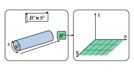
Figure 1: Illustrative representation of a four-dimensional spacetime with a compactified spatial dimension. The spacetime is composed by the compactified spatial dimension $z$, $S^{1}$, and a tridimensional space $R^{3}$ of coordinates $t,x,y$.

For the components of the complex field, $\varphi_{i}$, we apply the quasiperiodic condition feng2014casimir ; porfirio2021ground , i.e.,

$$\varphi_{i}\left(\tau,x,y,z+L\right)=e^{2i\pi\theta}\varphi_{i}\left(\tau,x,y,z\right).$$ (17)

This condition also compactifies the $z$-coordinate into a length $L$, but now there exists the influence of the phase $\theta$, that is, the quasiperiodic parameter that assumes values in the range $0\leq\theta<1$. In this sense, the quasiperiodic condition recovers the periodic one for $\theta=0$. The case for $\theta=1/2$ recovers the well known antiperiodic condition. Thereby, under the quasiperiodic condition, the eigenvalues of the operator $\hat{B}$, presented in Eq. (7), take the form

$$\beta_{\rho}=p_{\tau}^{2}+p_{x}^{2}+p_{y}^{2}+\frac{4\pi^{2}}{L^{2}}\left(n+\theta\right)^{2}+M_{g}^{2},\qquad\qquad M_{g}^{2}=\mu^{2}+g\Psi^{2},$$ (18)

where $n=0,\pm 1,\pm 2,...,$ and $\rho$ stands for the set of the quantum numbers $\left(p_{\tau},p_{x},p_{y},n\right)$. The values $\theta=0$ and $\theta=1/2$ are also known as the cases for the untwisted and twisted scalar fields, respectively.

Knowing the explicit form of the eigenvalues $\alpha_{\sigma}$ and $\beta_{\rho}$, given in Eqs. (16) and (18), respectively, one can construct the generalized zeta function from Eq. (8) and obtain a practical expression for the first order correction to the effective potential in Eq. (10). We shall do that next, also obtaining the topological mass.

III.1 One-loop correction

Starting from the eigenvalues presented in Eq. (16), which are associated with the real scalar field $\psi$, we construct the generalized zeta function from Eq. (8) as

$$\zeta_{\alpha}\left(s\right)=\frac{\Omega_{3}}{\left(2\pi\right)^{3}}\int dk_{\tau}dk_{x}dk_{y}\sum_{n=-\infty}^{+\infty}\left\{k_{\tau}^{2}+k_{x}^{2}+k_{y}^{2}+\left(\frac{2\pi n}{L}\right)^{2}+M_{\lambda}^{2}\right\}^{-s},$$ (19)

where $\Omega_{3}$ stands for the 3-dimensional volume associated with the Euclidean spacetime coordinates $\tau,x,y$, necessary to make the integrals dimensionless. In order to obtain an expression for the generalized zeta function (19), we shall follow similar steps as the ones presented in porfirio2021ground ; FariasJunior:2022qsp . We keep most of the calculation for the convenience of the reader. Thus, by using the identity,

$$w^{-s}=\frac{2}{\Gamma\left(s\right)}\int_{0}^{\infty}d\tau\ \tau^{2s-1}e^{-w\tau^{2}},$$ (20)

in Eq. (19) and performing the resulting Gaussian integrals in $k_{\tau}$, $k_{x}$ and $k_{z}$, one obtains the generalized zeta function in the form

$$\zeta_{\alpha}\left(s\right)=\frac{\Omega_{3}}{\left(2\pi\right)^{2}}\frac{\pi^{\frac{1}{2}}}{\Gamma\left(s\right)}\sum_{n=-\infty}^{+\infty}\int_{0}^{\infty}d\tau\ \tau^{2s-4}\exp\left\{-\tau^{2}\left[\left(\frac{2\pi n}{L}\right)^{2}+M_{\lambda}^{2}\right]\right\}.$$ (21)

The expression obtained in Eq. (21) is suited for the use of the well known integral representation of the gamma function $\Gamma\left(z\right)$ abramowitz1965handbook

$$\Gamma\left(z\right)=2\int_{0}^{\infty}d\mu\ \mu^{2z-1}e^{-\mu^{2}},$$ (22)

which allows us to rewrite the generalized zeta function (21) in terms only of the summation in $n$, i.e.,

$$\zeta_{\alpha}\left(s\right)=\frac{\Omega_{4}\pi^{\frac{3}{2}-2s}}{2^{2s}L^{4-2s}}\frac{\Gamma\left(s-\frac{3}{2}\right)}{\Gamma\left(s\right)}\sum_{n=-\infty}^{+\infty}\left[n^{2}+\left(\frac{M_{\lambda}L}{2\pi}\right)^{2}\right]^{\frac{3}{2}-s}.$$ (23)

The quantity $\Omega_{4}$ stands for the 4-dimensional volume in Euclidean spacetime, which takes into account the spacetime topology $S^{1}\times R^{3}$ as a consequence of the periodic condition imposed on the field. In the case under consideration, the 4-dimensional volume is written as $\Omega_{4}=\Omega_{3}L$. In order to perform the sum in Eq. (23) we use the following analytic continuation of the inhomogeneous generalized Epstein function elizalde1995zeta ; feng2014casimir ; FariasJunior:2022qsp :

$$\sum_{n=-\infty}^{+\infty}\left[\left(n+\vartheta\right)^{2}+\kappa^{2}\right]^{-z}=\frac{\pi^{\frac{1}{2}}\kappa^{1-2z}}{\Gamma\left(z\right)}\left\{\Gamma\left(z-\frac{1}{2}\right)+4(\pi\kappa)^{z-\frac{1}{2}}\sum_{j=1}^{\infty}j^{z-\frac{1}{2}}\cos\left(2\pi j\vartheta\right)K_{\left(\frac{1}{2}-z\right)}\left(2\pi j\kappa\right)\right\},$$ (24)

where $K_{\gamma}(x)$ is the modified Bessel function of the second kind or, as it is also known, the Macdonald function abramowitz1965handbook . After the use of Eq. (24), the generalized zeta function in Eq. (23) is presented in the form

$$\zeta_{\alpha}\left(s\right)=\frac{\Omega_{4}M_{\lambda}^{4-2s}}{2^{4}\pi^{2}\Gamma\left(s\right)}\left\{\Gamma\left(s-2\right)+2^{4-s}\sum_{j=1}^{\infty}f_{\left(2-s\right)}\left(jM_{\lambda}L\right)\right\},$$ (25)

where we have defined the function $f_{\mu}\left(x\right)$ as

$$f_{\gamma}\left(x\right)=\frac{K_{\gamma}\left(x\right)}{x^{\gamma}}.$$ (26)

By evaluating the generalized zeta function in Eq. (25) and its derivative with respect to $s$, in the limit $s\rightarrow 0$, one finds from Eq. (10) the one-loop contribution to the effective potential as

$$V_{\alpha}^{\left(1\right)}\left(\Psi\right)=\frac{M_{\lambda}^{4}}{64\pi^{2}}\left[\ln\left(\frac{M_{\lambda}^{2}}{\nu^{2}}\right)-\frac{3}{2}\right]-\frac{M_{\lambda}^{4}}{2\pi^{2}}\sum_{j=1}^{\infty}f_{2}\left(jM_{\lambda}L\right).$$ (27)

The expression above is the first order correction, that is, the one-loop correction to the effective potential due to the periodic condition. It remains to be evaluated the contribution due to the complex field for the one-loop correction, which we shall analyze below.

For the components of the complex scalar field, the eigenvalues are presented in Eq. (18), allowing us to construct the associated generalized zeta function in the form

$$\zeta_{\beta}\left(s\right)=\frac{\Omega_{3}}{\left(2\pi\right)^{3}}\int dp_{\tau}dp_{x}dp_{y}\sum_{n=-\infty}^{+\infty}\left[p_{\tau}^{2}+p_{x}^{2}+p_{y}^{2}+\frac{4\pi^{2}}{L^{2}}\left(n+\theta\right)^{2}+M_{g}^{2}\right]^{-s}.$$ (28)

The expression for the generalzized zeta function, $\zeta_{\beta}\left(s\right)$, arising due to a real scalar field has been obtained in detail in porfirio2021ground and, of course, for our case is very similar since the componentes of the complex field considered are real. Therefore, we present only the final result, i.e.,

$$\zeta_{\beta}\left(s\right)=\frac{\Omega_{4}M_{g}^{4-2s}}{16\pi^{2}\Gamma\left(s\right)}\left\{\Gamma\left(s-2\right)+2^{4-s}\sum_{j=1}^{\infty}\cos\left(2\pi j\theta\right)f_{\left(2-s\right)}\left(jM_{g}L\right)\right\}.$$ (29)

From Eq. (10) and using the generalized zeta function presented above, one is able to write the first order correction to the effective potential due to the complex field as

$$V_{\beta}^{\left(1\right)}\left(\Psi\right)=\frac{M_{g}^{4}}{32\pi^{2}}\left[\ln\left(\frac{M_{g}^{2}}{\nu^{2}}\right)-\frac{3}{2}\right]-\frac{M_{g}^{4}}{\pi^{2}}\sum_{j=1}^{\infty}\cos\left(2\pi j\theta\right)f_{2}\left(jM_{g}L\right).$$ (30)

Collecting the results presented in Eqs. (27) and (30), we can write the first order correction to the effective potential associated with the interacting real and complex scalar fields in the following form:

$$V^{\left(1\right)}\left(\Psi\right) = \frac{M_{\lambda}^{4}}{64\pi^{2}}\left[\ln\left(\frac{M_{\lambda}^{2}}{\nu^{2}}\right)-\frac{3}{2}\right]+\frac{M_{g}^{4}}{32\pi^{2}}\left[\ln\left(\frac{M_{g}^{2}}{\nu^{2}}\right)-\frac{3}{2}\right]+$$ (31)

$$-\frac{M_{\lambda}^{4}}{2\pi^{2}}\sum_{j=1}^{\infty}f_{2}\left(jM_{\lambda}L\right)-\frac{M_{g}^{4}}{\pi^{2}}\sum_{j=1}^{\infty}\cos\left(2\pi j\theta\right)f_{2}\left(jM_{g}L\right).$$

Therefore, from Eq. (9), the nonrenormalized effective potential up to one-loop correction reads

$$V_{\mathrm{eff}}\left(\Psi\right) = \frac{m^{2}+C_{2}}{2}\Psi^{2}+\frac{\lambda_{\psi}+C_{1}}{4!}\Psi^{4}+C_{3}+$$ (32)

$$+\frac{M_{\lambda}^{4}}{64\pi^{2}}\left[\ln\left(\frac{M_{\lambda}^{2}}{\nu^{2}}\right)-\frac{3}{2}\right]+\frac{M_{g}^{4}}{32\pi^{2}}\left[\ln\left(\frac{M_{g}^{2}}{\nu^{2}}\right)-\frac{3}{2}\right]+$$

$$-\frac{M_{\lambda}^{4}}{2\pi^{2}}\sum_{j=1}^{\infty}f_{2}\left(jM_{\lambda}L\right)-\frac{M_{g}^{4}}{\pi^{2}}\sum_{j=1}^{\infty}\cos\left(2\pi j\theta\right)f_{2}\left(jM_{g}L\right).$$

It is clear that the one-loop corrections in Eqs. (27) and (30) for the cases of real and complex fields, respectively, differ by a factor of two when $\theta=0$, the periodic condition particular case. This is justified since the complex field has two components. Note that the masses are also, in general, different. That is, for the real scalar field is $m$ and for the complex scalar field is $\mu$.

Once we obtain the effective potential $V_{\mathrm{eff}}\left(\Psi\right)$ in Eq. (32), our task is now to renormalize it. Hence, by following the renormalization procedure, from the conditions presented in Eqs. (11), (12) and (14), in the limit of Minkowski spacetime $L\rightarrow\infty$, one obtains the renormalization constants as

$$C_{1}=\frac{3\lambda_{\psi}^{2}}{32\pi^{2}}\ln\left(\frac{\nu^{2}}{m^{2}}\right)+\frac{3g^{2}}{4\pi^{2}}\ln\left(\frac{\nu^{2}}{m^{2}}\right),$$

$$C_{2}=\frac{\lambda_{\psi}m^{2}}{32\pi^{2}}\left[\ln\left(\frac{\nu^{2}}{m^{2}}\right)+1\right]+\frac{g\mu^{2}}{8\pi^{2}}\left[\ln\left(\frac{\nu^{2}}{\mu^{2}}\right)+1\right],$$

$$C_{3}=\frac{m^{4}}{64\pi^{2}}\left[\ln\frac{\nu^{2}}{m^{2}}+\frac{3}{2}\right]+\frac{\mu^{4}}{32\pi^{2}}\left[\ln\left(\frac{\nu^{2}}{\mu^{2}}\right)+\frac{3}{2}\right].$$ (33)

Furthermore, by substituting the renormalization constants above into the nonrenormalized effective potential given in Eq. (32), we are able to write the renormalized effective potential in the following form:

$$V_{\mathrm{eff}}^{R}\left(\Psi\right) = \frac{m^{2}}{2}\Psi^{2}+\frac{\lambda_{\psi}}{4!}\Psi^{4}+\frac{\mu^{4}}{32\pi^{2}}\ln\left(\frac{M_{g}^{2}}{\mu^{2}}\right)+\frac{m^{4}}{64\pi^{2}}\ln\left(\frac{M_{\lambda}^{2}}{m^{2}}\right)+$$ (34)

$$+\frac{g\mu^{2}\Psi^{2}}{16\pi^{2}}\left[\ln\left(\frac{M_{g}^{2}}{\mu^{2}}\right)-\frac{1}{2}\right]+\frac{\lambda_{\psi}^{2}\Psi^{4}}{256\pi^{2}}\left[\ln\left(\frac{M_{\lambda}^{2}}{m^{2}}\right)-\frac{3}{2}\right]+$$

$$+\frac{\lambda_{\psi}m^{2}\Psi^{2}}{64\pi^{2}}\left[\ln\left(\frac{M_{\lambda}^{2}}{m^{2}}\right)-\frac{1}{2}\right]+\frac{g^{2}\Psi^{4}}{32\pi^{2}}\left[\ln\left(\frac{M_{g}^{2}}{\mu^{2}}\right)-\frac{3}{2}\right]+$$

$$-\frac{M_{\lambda}^{4}}{2\pi^{2}}\sum_{j=1}^{\infty}f_{2}\left(jM_{\lambda}L\right)-\frac{M_{g}^{4}}{\pi^{2}}\sum_{j=1}^{\infty}\cos\left(2\pi j\theta\right)f_{2}\left(jM_{g}L\right).$$

The explicit form of the renormalized effective potential presented in Eq. (34) makes possible to evaluate the Casimir energy density and also the topological mass, up to first order correction.

In order to proceed and calculate the vacuum energy density, let us consider $\Psi=0$ as the stable vacuum state of the theory, although there are other possible stable vacuum states, as analyzed in Sec.III.3. Thus, from the renormalized effective potential $V_{\mathrm{eff}}^{R}\left(\Psi\right)$ in Eq. (34) one can evaluate the Casimir energy density in a straightforwardly way since the vacuum state is obtained by setting $\Psi=0$. Hence, the Casimir energy density is found to be

$$\mathcal{E}_{\mathrm{C}} = \left.V_{\mathrm{eff}}^{R}\left(\Psi\right)\right|_{\Psi=0}$$ (35)

$$= -\frac{m^{4}}{2\pi^{2}}\sum_{n=1}^{\infty}f_{2}\left(nmL\right)-\frac{\mu^{4}}{\pi^{2}}\sum_{j=1}^{\infty}\cos\left(2\pi j\theta\right)f_{2}\left(j\mu L\right).$$

Note that the first term on the r.h.s. of Eq. (35) is the contribution to the Casimir energy density from the real scalar field $\psi$ subjected to a periodic condition, while the second term is the contribution from the complex field subjected to a quasiperiodic condition porfirio2021ground . In the particular case, $\theta=0$, this contribution is twice the one from the real scalar field if the masses are equal. In order to show the influence of the complex field, under a quasiperiodic condition, on the Casimir energy density of the real field, we have plotted the expression in Eq. (35) as a function of $mL$ which is shown on the left side of Fig.2 for different values of $\theta$ and taken $\mu=m$. The black solid line is the Casimir energy density free of interaction with the complex field, only with the effect of the real field self-interaction. It is clear that depending on the value of the quasiperiodic parameter $\theta$, the Casimir energy density can be bigger or smaller than the free case, including the possibility of assuming positive or negative values. Note that the curves tend to repeat their behavior for values such that $\theta>0.5$. For instance, the curve represented by the green dot-dashed line for $\theta=0.3$ is the same as the one for $\theta=0.7$, and so on. Furthermore, all the curves end in their corresponding massless field constant value cases at $mL=0$, as it can be checked from Eq. (38). Also, in the regime $mL\gg 1$, the Casimir energy density in Eq. (35) goes to zero for all curves, as revealed by the plot on the left side of Fig.2. This a consequence of the exponentially suppressed behavior of the Macdonald function for large arguments abramowitz1965handbook .

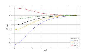
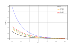
Figure 2: Plot of the dimensionless Casimir energy density, $E(mL)=2\pi^{2}L^{4}\mathcal{E}_{\mathrm{C}}$, defined from Eq. (35), as a function of $mL$, is shown on the left. The plot on the right shows the dimensionless two-loop contribution to the Casimir energy density, $E^{c}(mL)=32\pi^{4}L^{4}\Delta\mathcal{E}_{\mathrm{C}}$, defined from Eq. (48), as a function of $mL$ and considering $\lambda_{\psi}=10^{-2}$, $\lambda_{\varphi}=10^{-2}$ and $g=10^{-3}$. For both cases we have taken $\mu=m$ and different values of $\theta$.

It is interesting to consider the case of massless scalar fields, i.e., the limit $m,\mu\rightarrow 0$ of Eq. (35). For the massless scalar field case, we can make use of the limit for small arguments of the Macdonald function, i.e., $K_{\mu}\left(x\right)\simeq\frac{\Gamma\left(\mu\right)}{2}\left(\frac{2}{x}\right)^{\mu}$ abramowitz1965handbook . Hence, from Eq. (35), we obtain the Casimir energy density for interacting massless scalar fields as

$$\mathcal{E}_{\mathrm{C}}=-\frac{\pi^{2}}{90L^{4}}-\frac{2}{\pi^{2}L^{4}}\sum_{j=1}^{\infty}j^{-4}\cos\left(2\pi j\theta\right),$$ (36)

where we have used the following result for the Riemann zeta function $\zeta\left(4\right)=\frac{\pi^{4}}{90}$ elizalde1995zeta ; elizalde1995ten , on the first term on the r.h.s. of Eq. (36). This term is the already known Casimir effect result for a free massless scalar field subjected to a periodic condition toms1980symmetry . In addition, the second term on the r.h.s. of Eq. (36) can be rewritten in terms of the well known Bernoulli polynomials,

$$B_{2k}\left(\theta\right)=\frac{\left(-1\right)^{k-1}2\left(2k\right)!}{\left(2\pi\right)^{2k}}\sum_{n=1}^{\infty}\frac{\cos\left(2\pi n\theta\right)}{n^{2k}}.$$ (37)

Hence, the expression for the Casimir energy density, in the massless scalar fields case, is found to be

$$\mathcal{E}_{\mathrm{C}}=-\frac{\pi^{2}}{90L^{4}}+2\frac{\pi^{2}}{3L^{4}}\left(\theta^{4}-2\theta^{3}+\theta^{2}-\frac{1}{30}\right),$$ (38)

where we have made use of the Bernoulli polynomial of fourth order, that is, $B_{4}\left(\theta\right)=\left(\theta^{4}-2\theta^{3}+\theta^{2}-\frac{1}{30}\right)$. As one should expect, the first term on the r.h.s. of Eq. (38) is consistent with the result found in toms1980symmetry while the second term is consistent with the result found in feng2014casimir ; porfirio2021ground (taking into account the two components of the complex field). The latter also provides the right expressions for the periodic $\left(\theta=0\right)$ and antiperiodic $\left(\theta=\frac{1}{2}\right)$ cases, also known as untwisted and twisted cases, respectively.

We wish now to investigate the influence of the conditions in the mass $m$ of the real scalar field, i.e., the generation of topological mass at one-loop level. From the condition presented in Eq. (12) and making use of the renormalized effective potential (34), one obtains the following expression for the topological mass of the real scalar field $\psi$:

$$m_{T}^{2}=m^{2}\left[1+\frac{\lambda_{\psi}}{4\pi^{2}}\sum_{n=1}^{\infty}f_{1}\left(nmL\right)+\frac{\mu^{2}}{m^{2}}\frac{g}{\pi^{2}}\sum_{j=1}^{\infty}\cos\left(2\pi j\theta\right)f_{1}\left(j\mu L\right)\right].$$ (39)

Note that the topological mass $m_{T}^{2}$ does not present any divergencies, making possible for us to consider the massless field limit, that is, $m,\mu\rightarrow 0$. Hence, by using the same approximation for the Macdonald function as the one applied to obtain Eq. (36) from Eq. (35), we find the topological mass as

$$m_{T}^{2}=\frac{\lambda_{\psi}}{24L^{2}}+\frac{g}{L^{2}}\left(\theta^{2}-\theta+\frac{1}{6}\right).$$ (40)

In the expression above we have used the Riemann zeta function $\zeta\left(2\right)=\frac{\pi^{2}}{6}$ elizalde1995zeta ; elizalde1995ten and also the Bernoulli polynomials presented in Eq. (37), with $B_{2}\left(\theta\right)=\theta^{2}-\theta+\frac{1}{6}$. As one can see, the mass correction comes from the self-interaction term, which is proportional to $\lambda_{\psi}$, and also from the interaction between the fields, which is proportional to the coupling constant $g$. Note that the first term on the r.h.s. of Eq. (40) has been previously obtained in Ref. toms1980symmetry in a real scalar field theory with only self-interaction.

Another interesting aspect associated with the topological mass is that if $\lambda_{\psi}<g$, Eq. (40) may become negative depending on the value of $\theta$, which would in principle indicate vacuum instability. Had we, for instance, considered a complex scalar field theory with only self-interaction (no interaction between the fields) this would be a problem since it does not make sense to consider a constant complex field, $\Phi_{i}\neq 0$, compatible with the quasiperiodic condition for $\theta\neq 0$. The case $\theta=0$ is not problematic in this regard and that is why we have made the real scalar field to obey the periodic condition. Nevertheless, this problem is solved by taking into account an interaction theory as the one considered here (see also toms1980interacting ). Within this theory it is possible to study the vacuum stability, which in fact is made in Sec.III.3 by considering for simplicity a massless scalar field theory. The analysis indicates that the vacuum $\Psi=0$ is stable only if $\lambda_{\psi}>-24gB_{2}(\theta)$, otherwise it is necessary to consider the two other possible stable vacuum states, $\Psi_{\pm}$, in Eq. (55).

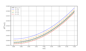
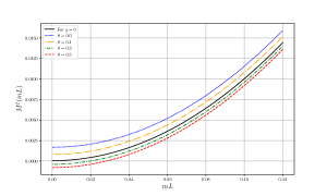
Figure 3: Plot of the dimensionless topological mass squared, $M^{2}(mL)=m_{T}^{2}L^{2}$, defined from Eq. (39), as a function of $mL$, for different values of $\theta$ and taken $\mu=m$. On the left, the plot shows the curves for $\lambda_{\psi}=10^{-2}$ and $g=10^{-3}$ while on the right the plot shows the curves for $\lambda_{\psi}=10^{-3}$ and $g=10^{-2}$.

In Fig.3 we have plotted the dimensionless mass squared, $M^{2}(mL)=m_{T}^{2}L^{2}$, defined from Eq. (39), as a function of $mL$, for different values of $\theta$ and taken $\mu=m$. On the left of Fig.3 the plot shows the curves for $\lambda_{\psi}=10^{-2}$ and $g=10^{-3}$, which satisfies the condition $\lambda_{\psi}>-24gB_{2}(\theta)$ in order $\Psi=0$ be a stable vacuum. This plot provides positive values in Eq. (40) for all values of the quasiperiodic parameter $\theta$, as we should expect. In contrast, the plot on the right shows the curves for $\lambda_{\psi}=10^{-3}$ and $g=10^{-2}$, which satisfies the condition $\lambda_{\psi}<-24gB_{2}(\theta)$. In this case, there exist negative values of Eq. (40) for $\theta=0.3$ and $\theta=0.5$, showing that $\Psi=0$ is in fact an unstable vacuum state. However, in a massive scalar field theory, $\Psi=0$, becomes stable for larger values of $mL$ even if $\lambda_{\psi}<g$, as indicates the plot on the right. Note that all curves, at $mL=0$, end in their corresponding constant massless scalar field values for the topological mass in Eq. (40). For large values of $mL$ the Macdonald function is exponentially suppressed and the curves are dominated by the first term on the r.h.s. of Eq. (39). Note also that the curves tend to repeat themselves for $\theta>0.5$.

The one-loop correction analysis is now done, so one can proceed to the two-loop correction contribution by still considering $\Psi=0$ as the stable vacuum state. As we now know, it means that we have to consider the restriction $\lambda_{\psi}>-24gB_{2}(\theta)$.

III.2 Two-loop correction

We want now to analyze the loop correction to the Casimir energy density obtained in Eqs. (35) and (36). This can be done by considering the second order correction to the effective potential, which can be obtained from the two-loop Feynman graphs. Since we have more than one contribution, we evaluate all the two-loop contributions from each Feynman graph separately. Hence, we write

$$V^{\left(2\right)}\left(\Psi\right)=V_{\lambda_{\psi}}^{\left(2\right)}\left(\Psi\right)+V_{\lambda_{\varphi}}^{\left(2\right)}\left(\Psi\right)+V_{g}^{\left(2\right)}\left(\Psi\right)+V_{2\lambda_{\varphi}}^{\left(2\right)}\left(\Psi\right),$$ (41)

where $V_{\lambda_{\psi}}^{\left(2\right)}$ is the contribution from the self-interaction term, $\frac{\lambda_{\psi}}{4!}\psi^{4}$, of the real field, $V_{\lambda_{\varphi}}^{\left(2\right)}$ is the contribution from the self-interaction of the complex field, that is, $\frac{\lambda_{\varphi}}{4!}\varphi_{1}^{4}$ and $\frac{\lambda_{\varphi}}{4!}\varphi_{2}^{4}$, $V_{g}^{\left(2\right)}$ is associated with the interaction between the real and complex fields $\frac{g}{2}\varphi_{1}^{2}\psi^{2}$ and $\frac{g}{2}\varphi_{2}^{2}\psi^{2}$ and, finally, $V_{2\lambda_{\varphi}}^{\left(2\right)}$ is associated with the cross terms of the components of the complex field $\frac{\lambda_{\varphi}}{4!}2\varphi_{1}^{2}\varphi_{2}^{2}$.

Figure 4: Feynman graph representing the only non-vanishing self-interaction contribution to the two-loop correction calculated at $\Psi=0$.

Let us first consider the contribution from the self-interaction term associated with the real field, $V_{\lambda_{\psi}}^{\left(2\right)}\left(\Psi\right)$. Since we are interested in the vacuum state where $\Psi=0$, the only nonvanishg contribution comes from the graph exhibited in Fig.4. With the help of this Feynman graph one can write the two-loop contribution in terms of the generalized zeta function presented in Eq. (25) in the following form FariasJunior:2022qsp ; porfirio2021ground :

$$V_{\lambda_{\psi}}^{\left(2\right)}\left(0\right)=\frac{\lambda_{\psi}}{8}\left.\left[\frac{\zeta_{\alpha}^{R}\left(1\right)}{\Omega_{4}}\right]^{2}\right|_{\Psi=0}.$$ (42)

The zeta function $\zeta_{\alpha}^{R}\left(s\right)$ is defined as the non-divergent part of the generalized zeta function given by Eq. (25), at $s=1$ FariasJunior:2022qsp ; porfirio2021ground , i.e.,

$$\zeta_{\alpha}^{R}\left(s\right)=\zeta_{\alpha}\left(s\right)-\frac{\Omega_{4}M_{\lambda}^{4-2s}}{16\pi^{2}}\frac{\Gamma\left(s-2\right)}{\Gamma\left(s\right)}.$$ (43)

Note that the term that is being subtracted in the above equation is independent of the parameter $L$, when divided by $\Omega_{4}$, characterizing the conditions and, as usual, should be dropped. Explicitly, one obtains the following result for the two-loop contribution due to the self-interaction term of the real field:

$$V_{\lambda_{\psi}}^{\left(2\right)}\left(0\right)=\frac{\lambda_{\psi}m^{4}}{32\pi^{4}}\left[\sum_{j=1}^{\infty}f_{1}\left(jmL\right)\right]^{2}.$$ (44)

The above result shows that the two-loop contribution is proportional to the coupling constant $\lambda_{\psi}$, as it should.

The second contribution, $V_{\lambda_{\varphi}}^{\left(2\right)}\left(\Psi\right)$, to the total two-loop correction in Eq. (41) can be read from the same graph as the one in Fig.4. We can construct the function $\zeta_{\beta}^{R}\left(s\right)$ from the generalized zeta function (29), subtracting the divergent part at $s=1$, and then obtain the contribution from the self-interaction of the complex field, that is,

$$V_{\lambda_{\varphi}}^{\left(2\right)}\left(0\right)=2\frac{\lambda_{\varphi}\mu^{4}}{32\pi^{4}}\left[\sum_{j=1}^{\infty}\cos\left(2\pi j\theta\right)f_{1}\left(j\mu L\right)\right]^{2},$$ (45)

which is proportional to $\lambda_{\varphi}$. The factor of two accounts for the two components of the complex field, that is, $\varphi_{1}$ and $\varphi_{2}$ that give rise to equal contributions.

Next we analyze the contributions from the interaction, $V_{g}^{\left(2\right)}\left(\Psi\right)$, between the fields. This correction can be read from the graph shown in Fig.5 and calculated, at $s=1$, by using the non-divergent part of the zeta functions in Eqs. (25) and (29). Hence, one finds the contribution from the interaction between the fields as

$$V_{g}^{\left(2\right)}\left(0\right)=2\frac{gm^{2}\mu^{2}}{8\pi^{4}}\left[\sum_{n=1}^{\infty}f_{1}\left(nmL\right)\right]\left[\sum_{j=1}^{\infty}\cos\left(2\pi j\theta\right)f_{1}\left(j\mu L\right)\right].$$ (46)

Since the expression (46) comes from the interaction term, it is proportional to the coupling constant $g$.

Figure 5: Feynman graph representing the only non-vanishing contribution to the two-loop correction, calculated at $\Psi=0$, due to the interaction between the real and complex fields. This graph also provides the only non-vanishing contribution due to the interaction of the components of the complex field. In this case, the solid line represents the propagator associated with the component $\varphi_{1}$ while the dashed line represents the propagator associated with the component $\varphi_{2}$.

Finally, the last contribution, $V_{2\lambda_{\varphi}}^{\left(2\right)}\left(\Psi\right)$, comes from the interaction of the components of the complex field (also a self-interaction). The contribution from this term is obtained from the graph in Fig.5, considering the solid line as representing the propagator associated with the field $\varphi_{1}$ and the dashed one associated with the field $\varphi_{2}$. Then, by using again the non-divergent part of the zeta function (29), calculated at $s=1$, the result is written as

$$V_{2\lambda_{\varphi}}^{\left(2\right)}\left(0\right)=\frac{\lambda_{\varphi}\mu^{4}}{48\pi^{4}}\left[\sum_{j=1}^{\infty}\cos\left(2\pi j\theta\right)f_{1}\left(j\mu L\right)\right]^{2}.$$ (47)

Note that, likewise the result presented in Eq. (45), the above expression is proportional to $\lambda_{\varphi}$.

Collecting all the results obtained in Eqs (44), (46), (45) and (47), one can write the total two-loop correction to the effective potential in Eq. (41), at the vacuum state $\Psi=0$, as

$$\Delta\mathcal{E}_{\mathrm{C}} = \left.V^{\left(2\right)}\left(\Psi\right)\right|_{\Psi=0}$$ (48)

$$= \frac{\lambda_{\psi}m^{4}}{32\pi^{4}}\left[\sum_{j=1}^{\infty}f_{1}\left(jmL\right)\right]^{2}+\frac{\lambda_{\varphi}\mu^{4}}{12\pi^{4}}\left[\sum_{j=1}^{\infty}\cos\left(2\pi j\theta\right)f_{1}\left(j\mu L\right)\right]^{2}+$$

$$+\frac{gm^{2}\mu^{2}}{4\pi^{4}}\left[\sum_{n=1}^{\infty}f_{1}\left(nmL\right)\right]\left[\sum_{j=1}^{\infty}\cos\left(2\pi j\theta\right)f_{1}\left(j\mu L\right)\right].$$

Therefore, combining the results presented in Eqs. (35) and (48), one obtains a correction to the Casimir energy density in Eq. (35), which is first order in all coupling constants of the theory. As we can notice, while the first order correction to the efective potential gives the Casimir energy density associated with a free scalar and complex fields theory, the second order correction to the effective potential in Eq. (48) provides a contribution to the Casimir energy density that is linearly proportional to all coupling constants.

Moreover, one can also consider the massless scalar fields limit of Eq. (48), that is, $\mu,m\rightarrow 0$. This gives

$$\Delta\mathcal{E}_{\mathrm{C}}=\frac{\lambda_{\psi}}{1152L^{4}}+\frac{\lambda_{\varphi}}{12L^{4}}\left(\theta^{2}-\theta+\frac{1}{6}\right)^{2}+\frac{g}{24L^{4}}\left(\theta^{2}-\theta+\frac{1}{6}\right).$$ (49)

Hence, the expression above is the first order correction, in all coupling constants of the theory, to the massless Casimir energy density in Eq. (38). Note that the first term on the r.h.s. of Eq. (49) has been obtained in Ref. toms1980symmetry , whilst the second term is consistent with the result obtained in Ref. porfirio2021ground in a real scalar field theory considering only self-interaction. In contrast, the third term is a new one arising from the interaction between the fields.

In Fig.2, the plot on the right shows the influence of the complex field, under a quasiperiodic condition, on the correction (48) to the Casimir energy density. Thus, the expression in Eq. (48) has been plotted as a function of $mL$, for different values of $\theta$ and taken $\mu=m$. We also have considered $\lambda_{\psi}=10^{-2}$, $\lambda_{\varphi}=10^{-2}$ and $g=10^{-3}$. The black solid line is the correction free of interaction with the complex field, only with the effect of the real field self-interaction. It is clear that the curves for $\theta\neq 0$ increase the correction when compared to the black solid line. Note that the curves here also tend to repeat their behavior for values such that $\theta>0.5$. For instance, the curve represented by the orange dot-dashed line for $\theta=0.3$ is the same as the one for $\theta=0.7$. Furthermore, all the curves tend to their corresponding massless field constant value cases at $mL=0$, as it can be checked from Eq. (49). Also, in the regime $mL\gg 1$, the correction in Eq. (48) goes to zero for all curves, as revealed by the plot on the right side of Fig.2. This a consequence of the exponentially suppressed behavior of the Macdonald function for large arguments abramowitz1965handbook .

Next, we shall analyze the vacuum stability of the theory, since the state $\Psi=0$ is not the only possible vacuum state, as we have already anticipated.

III.3 Vacuum stability

We want to analyze here the stability of the possible vacuum states associated with the effective potential, up to first order loop correction, of the theory described by the action in Eq. (1). For simplicity we consider the case where the fields are massless, i.e., $m,\mu\rightarrow 0$. It is import to point out again that, for the complex scalar field obeying the condition in Eq. (17), the only constant field that can satisfy such a condition is the zero field, hence, we set $\Phi_{i}=0$. This fact also turns the approximation discussed below Eq. (2) into an exact expression, namely, the one in Eq. (5), which does not consider cross terms.

By following the same steps as the ones to obtain Eq. (32), the nonrenormalized effective potential for the massless scalar fields case is written as

$$V_{\mathrm{eff}}\left(\Psi\right)=\frac{\lambda_{\psi}+C}{4!}\Psi^{4}+\frac{\lambda_{\psi}^{2}\Psi^{4}}{256\pi^{2}}\left[\ln\left(\frac{\lambda_{\psi}\Psi^{2}}{2\nu^{2}}\right)-\frac{3}{2}\right]+\frac{g^{2}\Psi^{4}}{32\pi^{2}}\left[\ln\left(\frac{g\Psi^{2}}{\nu^{2}}\right)-\frac{3}{2}\right]+$$

$$-\frac{\lambda_{\psi}^{2}\Psi^{4}}{8\pi^{2}}\sum_{j=1}^{\infty}f_{2}\left(j\sqrt{\frac{\lambda_{\psi}}{2}\Psi^{2}}L\right)-\frac{g^{2}\Psi^{4}}{\pi^{2}}\sum_{j=1}^{\infty}\cos\left(2\pi j\theta\right)f_{2}\left(j\sqrt{g\Psi^{2}}L\right).$$ (50)

Furthermore, the condition which takes care of the renormalization constant $C$, is given by Eq. (11). Thereby, by applying this condition on the effective potential of Eq. (50), in the Minkowski limit $L\rightarrow\infty$, one finds that the constant $C$ is given by

$$C=\frac{3\lambda_{\psi}^{2}}{32\pi^{2}}\ln\left(\frac{2\nu^{2}}{\lambda_{\psi}M^{2}}\right)+\frac{3g^{2}}{4\pi^{2}}\ln\left(\frac{\nu^{2}}{gM^{2}}\right)-\frac{\lambda_{\psi}^{2}}{4\pi^{2}}-\frac{2g^{2}}{\pi^{2}}.$$ (51)

Next, by substituting $C$ in the effective potential (50), we obtain the renormalized effective potential for the massless scalar fields theory, i.e.,

$$V_{\mathrm{eff}}^{R}\left(\Psi\right)=\frac{\lambda_{\psi}}{4!}\Psi^{4}+\left[\frac{\lambda_{\psi}^{2}}{8}+g^{2}\right]\frac{\Psi^{4}}{32\pi^{2}}\ln\left(\frac{\Psi^{2}}{M^{2}}\right)-\left[\frac{\lambda_{\psi}^{2}}{8}+g^{2}\right]\frac{25\Psi^{4}}{192\pi^{2}}+$$

$$-\frac{\lambda_{\psi}^{2}\Psi^{4}}{8\pi^{2}}\sum_{j=1}^{\infty}f_{2}\left(j\sqrt{\frac{\lambda_{\psi}}{2}\Psi^{2}}L\right)-\frac{g^{2}\Psi^{4}}{\pi^{2}}\sum_{j=1}^{\infty}\cos\left(2\pi j\theta\right)f_{2}\left(j\sqrt{g\Psi^{2}}L\right).$$ (52)

Let us now investigate the possible vacuum states of the above renormalized effective potential, up to first order in the coupling constants $\lambda_{\psi}$ and $g$, which is more than enough since we have considered corrections to the Casimir energy density as well as to the mass of the scalar field only up to first order in the coupling constants. Thus, expanding the renormalized effective potential given by Eq. (52) in powers of $\lambda_{\psi}$ and $g$ toms1980interacting , up to first order, results in the following expression:

$$V_{\mathrm{eff}}^{R}\left(\Psi\right)\simeq-\frac{\pi^{2}}{90L^{4}}+\frac{2\pi^{2}}{3L^{4}}B_{4}\left(\theta\right)+\frac{\lambda_{\psi}}{4!}\Psi^{4}+\frac{\Psi^{2}}{48L^{2}}\left[\lambda_{\psi}+24gB_{2}\left(\theta\right)\right],$$ (53)

where $B_{4}\left(\theta\right)$ and $B_{2}\left(\theta\right)$ are the Bernoulli polynominals defined in Eq. (37). The minimum of the potential, which corresponds to the vacuum state, is obtained as usual by taking its derivative and equating the resulting expression to zero, that is,

$$\frac{\lambda_{\psi}}{6}\Psi^{3}+\frac{\Psi}{24L^{2}}\left[\lambda_{\psi}+24gB_{2}\left(\theta\right)\right]=0.$$ (54)

The roots of Eq. (54) represent possible vacuum states and are given by

$$\Psi=0,\qquad\qquad\Psi_{\pm}=\pm\sqrt{-\frac{1}{4\lambda_{\psi}L^{2}}\left[\lambda_{\psi}+24gB_{2}\left(\theta\right)\right]}.$$ (55)

In order to know which solution above may be a physical vacuum state, one has to analyze the stability of the effective potential (53). This is achieved by means of its second derivative, i.e.,

$$\frac{d^{2}V^{R}_{\mathrm{eff}}\left(\Psi\right)}{d\Psi^{2}}=\frac{\lambda_{\psi}}{2}\Psi^{2}+\frac{1}{24L^{2}}\left[\lambda_{\psi}+24gB_{2}\left(\theta\right)\right].$$ (56)

For the vacuum state to be stable the second derivative of the potential, evaluated at (55), must be greater than zero. In this sense, we investigate for which values of the parameter $\theta$ of the quasiperiodic condition and of the coupling constants the stability is achieved.

Let us then first consider the vacuum state, $\Psi=0$, which is the case considered previously in the analysis of the Casimir energy density, its loop correction and the topological mass. Hence, from Eq. (56), one sees that $\Psi=0$ is stable only if the following condition is satisfied:

$$\lambda_{\psi}>-24gB_{2}\left(\theta\right).$$ (57)

As we can see, the parameter $\theta$ plays a crucial role in determining whether or not this vacuum state is stable. Additionally, the coupling constants has also a great influence in the vacuum stability. Thus, by taking the coupling constants, $\lambda_{\psi}$ and $g$, to be positive, and for $B_{2}\left(\theta\right)$ also positive, the condition above is always satisfied. However, if $B_{2}\left(\theta\right)$ is negative the condition in Eq. (57) may be violated if $\lambda_{\psi}<g$. In Fig.6 we have plotted the Bernoulli polynomial $B_{2}\left(\theta\right)$, from where we can see its positive and negative values.

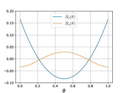
Figure 6: Bernoulli polynomials $B_{2}(\theta)$, solid line, and $B_{4}(\theta)$, dashed line, as functions of the quasiperiodic parameter $\theta$.

By using the explicit form of the Bernoulli polynomial, that is, $B_{2}\left(\theta\right)=\theta^{2}-\theta+\frac{1}{6}$, one finds that its negative values are provided for values of $\theta$ in the interval

$$\frac{1}{2}-\frac{\sqrt{3}}{6}<\theta<\frac{1}{2}+\frac{\sqrt{3}}{6}.$$ (58)

Of course, the values of $\theta$ for which $B_{2}(\theta)$ is positive reside out of the above interval.

As an example, let us consider the particular case where $\theta=0.5$. Hence, the condition of stability written in Eq. (57) becomes

$$\lambda_{\psi}>2g.$$ (59)

The above condition is in agreement with the one found in toms1980interacting . Note, however, that we are considering a complex scalar field. The topological mass, in this case, takes the following form:

$$m_{T}^{2}=\frac{\left(\lambda_{\psi}-2g\right)}{24L^{2}},$$ (60)

which agrees with the result obtained in Eq. (40) for $\theta=0.5$. Note also that if the interaction between the fields is not presente, that is, $g=0$, we recover the previous known result found in Refs. Ford:1978ku ; toms1980symmetry .

According to Eq. (55) it is also possible to consider, $\Psi=\Psi_{\pm}$, as the vacuum states, instead of $\Psi=0$. In this case, evaluating the second derivative of the potential in Eq. (56), at $\Psi=\Psi_{\pm}$, and setting the result to be greater than zero, one obtains the vacuum stability condition as

$$\lambda_{\psi}<-24gB_{2}\left(\theta\right).$$ (61)

For positive coupling constants, the above condition is satisfied only if the Bernoulli polynomial, $B_{2}\left(\theta\right)$, is negative. This is in fact possible for values of $\theta$ in the interval (58). By considering the same example as before, that is, $\theta=0.5$, we obtain the stability condition for a twisted scalar field as

$$\lambda_{\psi}<2g.$$ (62)

Consequently, the topological mass for this case reads

$$m_{T}^{2}=\frac{2g-\lambda_{\psi}}{12L^{2}}.$$ (63)

Note that the above result for the topological mass differs from the one presented in Eq. (40) for $\theta=0.5$. This difference arises from the fact that the considered stable vacuum state for Eq. (63), that is, $\Psi=\Psi_{\pm}$, is not the same as the one in Eq. (40), that is, $\Psi=0$. For the latter to be stable, as we have seen above, it is necessary to consider the restriction in Eq. (57). The result in Eq. (63) is in agreement with the one found in Ref. toms1980symmetry .

The Casimir energy density can also be obtained by taking, $\Psi=\Psi_{\pm}$, as the stable vacuum state. Thus, from Eq. (55), the effective potential given by Eq (53) provides the following expression for the Casimir energy density:

$$\mathcal{E}_{C} = \left.V^{R}_{\mathrm{eff}}\left(\Psi\right)\right|_{\Psi_{\pm}}$$ (64)

$$\simeq -\frac{\pi^{2}}{90L^{4}}+2\frac{\pi^{2}}{3L^{4}}B_{4}\left(\theta\right)-\frac{1}{384\lambda_{\psi}L^{4}}\left[\lambda_{\psi}+24gB_{2}\left(\theta\right)\right]^{2}.$$

Note that the first two terms on the r.h.s. of Eq. (64) are in agreement with the Casimir energy density presented in Eq. (38). However, the third term presents a dependency on the coupling constants $\lambda_{\psi}$ and $g$, which does not appear in the case where the stable vacuum state is $\Psi=0$. It is important to point out that Eq. (64) is only an approximation, up to first order in the coupling constants, since we are taking into account the expansion of the effective potential presented in Eq. (53). The first and third terms are always negative, while the second term can be positive or negative, depending on the value of the Bernoulli Polynomial $B_{4}\left(\theta\right)$, shown in Fig.6.

In order to calculate the two-loop correction contribution to the Casimir energy density in Eq. (64) would be necessary to consider additional Feynman graphs other than the ones shown in Figs.4, 5. These additional Feynman graphs come from the second term on the r.h.s. of Eq. (24) in Ref. toms1980symmetry , which vanishes in the case $\Psi=0$ is the stable vacuum state. The consideration of the two-loop contribution, of course, would make our problem extremely difficult so that we restrict our analysis only to the one-loop correction that provides the Casimir energy density in Eq. (64).

From Eqs. (57) and (61), we can conclude that the stability of the vacuum states is determined by the values of the coupling constants $\lambda_{\psi}$ and $g$, as well as by the value of the parameter $\theta$ of the quasiperiodic condition for the complex field. However there is no dependency on the parameter $L$.

In the next section we consider the same system as the one considered in this section, but the complex field is now subjected to mixed boundary conditions.

IV Periodic condition and mixed boundary conditions

In this section we consider the real scalar field obeying periodic condition as before, but now the complex scalar field is subject to mixed boundary conditions. In practice, the first order loop correction to the effective potential associated with the real scalar field is the same as in Eq. (27), differently from the complex field which yields a different contribution since it obeys a different condition. In this case, it is sufficient to evaluate only the correction associated with the complex field. We will also assume that $\Psi=0$ is the stable vacuum state for the analysis below, although a discussion of other possible stable vacuum states is given in Sec.IV.3.

The complex field real components are subject to the following mixed boundary conditions applied on the planes shown in Fig.7 barone2004radiative ; cruz2020casimir ; Ferreira:2023uxs :

$$\left.\varphi_{i}\left(w\right)\right|_{z=0}=\left.\frac{\partial\varphi_{i}\left(w\right)}{\partial z}\right|_{z=L},\qquad\qquad\left.\frac{\partial\varphi_{i}\left(w\right)}{\partial z}\right|_{z=0}=\left.\varphi_{i}\left(w\right)\right|_{z=L},$$ (65)

where $w=(\tau,x,y,z)$. By taking into account the boundary conditions above, the eigenvalues of the operator $\hat{B}$ given in Eq. (7), takes the form barone2004radiative ; cruz2020casimir

$$\beta_{\rho}=k_{\tau}^{2}+k_{x}^{2}+k_{y}^{2}+\left(n+\frac{1}{2}\right)^{2}\frac{\pi^{2}}{L^{2}}+M_{g}^{2},\qquad\qquad M_{g}^{2}=\mu^{2}+g\Psi^{2},$$ (66)

where $n=0,1,2,...,$ and the subscript $\rho$ stands for the set of quantum numbers $\left(k_{\tau},k_{x},k_{y},n\right)$. It is worth pointing out that, from Eq. (65), two configurations are possible on the parallel planes in Fig.7. For the plane at $z=0$ we can have Dirichlet boundary condition while for the plane at $z=L$ we can have the Neumann one. Conversely, for the plane at $z=0$ we can have Neumann boundary condition while for the plane at $z=L$ we can have the Dirichlet one. However, both configurations provide the same eigenvalues in Eq. (66).

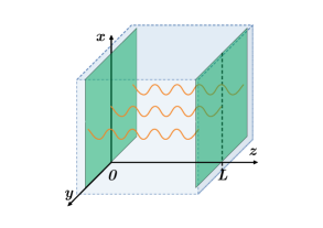
Figure 7: Two identical and perfectly reflecting parallel planes placed at $z=0$ and $z=L$, confining the field modes of a complex scalar field. On the planes the mixed boundary conditions in Eq. (65) are applied.

Having the eigenvalues obtained in Eq. (66) we can now proceed to the investigation of the first order correction, that is, the one-loop correction to the effective potential associated with the complex scalar field subjected to mixed boundary conditions on the planes shown in Fig.7.

IV.1 One-loop correction

The required steps for the obtention of the generalized zeta function for the case under consideration, goes in a similar way as the one presentend in the previous sections and also in cruz2020casimir . Therefore, we present only the main steps for the reader’s convenience. Constructing the generalized zeta function with the eigenvalues presented in (66) requires the use of the identity in Eq. (20) which, after the integration of the momenta, one can use the integral representation of the gamma function, (22), finding the expression

$$\zeta_{\beta}\left(s\right)=\frac{\Omega_{4}\pi^{\frac{3}{2}-2s}}{8L^{4-2s}}\frac{\Gamma\left(s-\frac{3}{2}\right)}{\Gamma\left(s\right)}\sum_{n=0}^{+\infty}\left[\left(n+\frac{1}{2}\right)^{2}+\left(\frac{M_{g}L}{\pi}\right)^{2}\right]^{\frac{3}{2}-s},$$ (67)

where $\Omega_{4}$ is the 4-dimensional volume written as $\Omega_{4}=\Omega_{3}L$, with $\Omega_{3}$ being the 3-dimensional volume associated with the Euclidean spacetime coordinates $\tau,x,y$. In order to perform the sum in Eq. (67), we write it as a sum of two terms cruz2020casimir ; bordag2009advances , i.e.,

$$\sum_{n=0}^{+\infty}\left[\left(n+\frac{1}{2}\right)^{2}+\vartheta^{2}\right]^{\frac{3}{2}-s}=\frac{1}{2^{3-2s}}\left\{\sum_{n=1}^{\infty}\left[n^{2}+\left(2\vartheta\right)^{2}\right]^{\frac{3}{2}-s}-2^{3-2s}\sum_{n=1}^{\infty}\left[n^{2}+\vartheta^{2}\right]^{\frac{3}{2}-s}\right\}.$$ (68)

Each sum on the r.h.s. of Eq. (68) can be written in terms of the Epstein-Hurwitz zeta function gradshteyn2014table

$$\zeta_{EH}\left(z,\kappa\right) = \sum_{n=1}^{+\infty}\left(n^{2}+\kappa^{2}\right)^{-z}$$ (69)

$$= -\frac{\kappa^{-2z}}{2}+\frac{\pi^{\frac{1}{2}}}{2}\frac{\Gamma\left(z-\frac{1}{2}\right)}{\Gamma\left(z\right)}\kappa^{1-2z}+\frac{2^{1-z}\left(2\pi\right)^{2z-\frac{1}{2}}}{\Gamma\left(z\right)}\sum_{n=1}^{\infty}n^{2z-1}f_{\left(z-\frac{1}{2}\right)}\left(2\pi n\kappa\right).$$

Hence, with the help of the Eq. (69) one obtains the generalized zeta function as

$$\zeta_{\beta}\left(s\right)=\frac{\Omega_{4}}{16\pi^{2}\Gamma\left(s\right)}\left\{M_{g}^{4-2s}\Gamma\left(s-2\right)+\frac{2^{s}}{L^{4-2s}}\sum_{n=1}^{\infty}n^{2s-4}\left[2^{2s-3}f_{\left(s-2\right)}\left(4nM_{g}L\right)-f_{\left(s-2\right)}\left(2nM_{g}L\right)\right]\right\}.$$ (70)

Evaluating the above expression and its derivative in the limit $s\rightarrow 0$, one finds the complex field contribution to the first order loop correction to the effective potential from Eq. (10), i.e.,

$$V_{\beta}^{\left(1\right)}\left(\Psi\right)=\frac{M_{g}^{4}}{32\pi^{2}}\left[\ln\left(\frac{M_{g}^{2}}{\nu^{2}}\right)-\frac{3}{2}\right]-\frac{M_{g}^{4}}{\pi^{2}}\sum_{n=1}^{\infty}\left[2f_{2}\left(4nM_{g}L\right)-f_{2}\left(2nM_{g}L\right)\right].$$ (71)

Taking into consideration the contribution from the real field, Eq. (27), along with the contribution above of the complex field, the effective potential, up to one-loop correction, is presented in the form

$$V_{\mathrm{eff}}\left(\Psi\right) = \frac{m^{2}+C_{2}}{2}\Psi^{2}+\frac{\lambda_{\psi}+C_{1}}{4!}\Psi^{4}+C_{3}+$$ (72)

$$+\frac{M_{\lambda}^{4}}{64\pi^{2}}\left[\ln\left(\frac{M_{\lambda}^{2}}{\nu^{2}}\right)-\frac{3}{2}\right]+\frac{M_{g}^{4}}{32\pi^{2}}\left[\ln\left(\frac{M_{g}^{2}}{\nu^{2}}\right)-\frac{3}{2}\right]+$$

$$-\frac{M_{\lambda}^{4}}{2\pi^{2}}\sum_{j=1}^{\infty}f_{2}\left(jM_{\lambda}L\right)-\frac{M_{g}^{4}}{\pi^{2}}\sum_{n=1}^{\infty}\left[2f_{2}\left(4nM_{g}L\right)-f_{2}\left(2nM_{g}L\right)\right].$$

Knowing the effective potential expressed in Eq. (72), one needs to renormalize it. Hence, by applying the renormalization conditions given by Eqs. (11), (12) and (14), we find the renormalization constants $C_{i}$ as the same as the ones obtained in Eq. (33), as it should be. After the substitution of these constants $C_{i}$’s in the effective potential, (72), one can write the renormalized effective potential as

$$V_{\mathrm{eff}}^{R}\left(\Psi\right) = \frac{m^{2}}{2}\Psi^{2}+\frac{\lambda_{\psi}}{4!}\Psi^{4}+\frac{\mu^{4}}{32\pi^{2}}\ln\left(\frac{M_{g}^{2}}{\mu^{2}}\right)+\frac{m^{4}}{64\pi^{2}}\ln\left(\frac{M_{\lambda}^{2}}{m^{2}}\right)+$$ (73)

$$+\frac{g\mu^{2}\Psi^{2}}{16\pi^{2}}\left[\ln\left(\frac{M_{g}^{2}}{\mu^{2}}\right)-\frac{1}{2}\right]+\frac{\lambda_{\psi}^{2}\Psi^{4}}{256\pi^{2}}\left[\ln\left(\frac{M_{\lambda}^{2}}{m^{2}}\right)-\frac{3}{2}\right]+$$

$$+\frac{\lambda_{\psi}m^{2}\Psi^{2}}{64\pi^{2}}\left[\ln\left(\frac{M_{\lambda}^{2}}{m^{2}}\right)-\frac{1}{2}\right]+\frac{g^{2}\Psi^{4}}{32\pi^{2}}\left[\ln\left(\frac{M_{g}^{2}}{\mu^{2}}\right)-\frac{3}{2}\right]+$$

$$-\frac{M_{\lambda}^{4}}{2\pi^{2}}\sum_{j=1}^{\infty}f_{2}\left(jM_{\lambda}L\right)-\frac{M_{g}^{4}}{\pi^{2}}\sum_{n=1}^{\infty}\left[2f_{2}\left(4nM_{g}L\right)-f_{2}\left(2nM_{g}L\right)\right].$$

Once we obtain the renormalized effective potential found in Eq. (73), the Casimir energy density is written in a straightforwardly way by setting $\Psi=0$, i.e.,

$$\mathcal{E}_{\mathrm{C}}=\left.V_{\mathrm{eff}}^{R}\left(\Psi\right)\right|_{\Psi=0}=-\frac{m^{4}}{2\pi^{2}}\sum_{j=1}^{\infty}f_{2}\left(jmL\right)-\frac{\mu^{4}}{\pi^{2}}\sum_{n=1}^{\infty}\left[2f_{2}\left(4n\mu L\right)-f_{2}\left(2n\mu L\right)\right].$$ (74)

The first term on the r.h.s. of Eq. (74) is the contribution from the real field which is equal to the one in Eq. (35) as it should, since the boundary condition applied to the real field is the same. However, the second term on the r.h.s. of Eq. (74) is the contribution from the complex field and differs from the case of quasiperiodic condition presented in Eq. (35). This contribution is consistent with the result shown in Ref. barone2004radiative where the authors considered a self-interacting real scalar field.

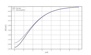
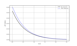
Figure 8: Plot of the dimensionless Casimir energy density, $E(mL)=2\pi^{2}L^{4}\mathcal{E}_{\mathrm{C}}$, defined from Eq. (74), as a function of $mL$ is shown on the left, while the plot on the right shows the dimensionless two-loop contribution to the Casimir energy density, $E^{c}(mL)=32\pi^{4}L^{4}\Delta\mathcal{E}_{\mathrm{C}}$, defined from Eq. (81), as a function of $mL$ and considering $\lambda_{\psi}=10^{-2}$, $\lambda_{\varphi}=10^{-2}$ and $g=10^{-3}$. For both cases we have taken $\mu=m$.

The massless scalar field case is obtained by taking the limit for small arguments of the Macdonald function abramowitz1965handbook . This yields the following Casimir energy density:

$$\mathcal{E}_{\mathrm{C}} = -\frac{\pi^{2}}{90L^{4}}\left[1-\frac{7}{64}\right]$$ (75)

$$= \frac{57}{64}\times\left(-\frac{\pi^{2}}{90L^{4}}\right),$$

where we can see that the effect of the interaction with the complex field subjected to mixed boundary conditions is to increase the Casimir energy density of the real scalar field under a periodic condition.

In Fig.8 we have plotted the Casimir energy density in Eq. (74) as a function of $mL$ and taken $m=\mu$, showing it on the left side. The latter shows how the curve for the free real scalar field (black solid line) differs from the curve when considering the influence of the interaction (blue dotted line). In fact, the interaction increases the value of the Casimir energy density, as shown the curves. This plot also shows that the Casimir energy density goes to zero for large values of $mL$. This a consequence of the exponentially suppressed behavior of the Macdonald function for large arguments abramowitz1965handbook . Also, the two curves end in their corresponding massless field constant value cases at $mL=0$, as it can be checked from Eq. (75).

Let us now investigate how the topological mass associated with the real field changes under the influence of mixed boundary conditions imposed on the complex field. Thus, applying the renormalization condition (12), with the renormalized effective potential in Eq. (73), provides the topological mass written as

$$m_{T}^{2}=m^{2}\left\{1+\frac{\lambda_{\psi}}{4\pi^{2}}\sum_{j=1}^{\infty}f_{1}\left(jmL\right)+\frac{\mu^{2}}{m^{2}}\frac{g}{\pi^{2}}\sum_{n=1}^{\infty}\left[2f_{1}\left(4n\mu L\right)-f_{1}\left(2n\mu L\right)\right]\right\}.$$ (76)

Of course the difference between the above result and the topological mass found in Eq. (39), relies in the third term on the r.h.s. of Eq. (76). Furthermore, by considering the massless scalar fields case, $m,\mu\rightarrow 0$, one obtains the topological mass as follows

$$m_{T}^{2}=\frac{2\lambda_{\psi}-g}{48L^{2}}.$$ (77)

Note that the topological mass above coincides with the particular cases of quasiperiodic condition in Eq. (40), for $\theta=1/4,3/4$, which are in the range of Eq. (58).

Similarly to the discussion presented in the previous section, here the topological mass squared can also become negative depending on whether $\lambda_{\psi}$ is bigger or smaller than $g$. For instance, if $2\lambda_{\psi}<g$, Eq. (77) becomes negative, indicating vacuum instability. Again, had we considered a complex scalar field theory with only self-interaction (no interaction between the fields) this would be a problem since it does not make sense to consider a constant complex field, $\Phi_{i}\neq 0$, compatible with mixed boundary conditions. This problem is solved by taking into account an interaction theory as the one considered in the present section (see also toms1980interacting ). Within this theory it is possible to study the vacuum stability, which here is made in Sec.IV.3 for massless scalar fields. The analysis indicates that the vacuum $\Psi=0$ is stable only if $2\lambda_{\psi}>g$, otherwise it is necessary to consider the two other possible vacuum states, $\Psi_{\pm}$, in Eq. (86).

In Fig.9, we have plotted the dimensionless mass squared, $M^{2}(mL)=m_{T}^{2}L^{2}$ , defined from Eq. (76), as a function of $mL$, taken $\mu=m$. On the left of Fig.9 the plot shows the curves for $\lambda_{\psi}=10^{-2}$ and $g=10^{-3}$, which satisfies the condition $2\lambda_{\psi}>g$ in order $\Psi=0$ be a stable vacuum. In contrast, the plot on the right shows the curves for $\lambda_{\psi}=10^{-3}$ and $g=10^{-2}$, which satisfies the condition $2\lambda_{\psi}<g$ . In this case, Eq. (77) becomes negative, showing that $\Psi=0$ is in fact an unstable vacuum state. Note that in an interacting massive scalar field theory $\Psi=0$ may still be a stable vacuum state even if $2\lambda_{\psi}<g$ for large values of $mL$, as shown in the plot on the right side. Note also that each curve, at $mL=0$, end in their corresponding constant massless scalar field values for the topological mass in Eq. (77). For large values of $mL$ the Macdonald function is exponentially suppressed and the curves are dominated by the first term on the r.h.s. of Eq. (76).

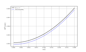
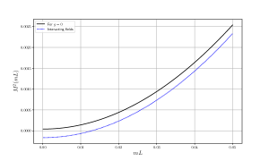
Figure 9: Plot of the dimensionless topological mass squared, $M^{2}(mL)=m_{T}^{2}L^{2}$, defined from Eq. (76), as a function of $mL$, taken $\mu=m$. On the left, the plot shows the curves for $\lambda_{\psi}=10^{-2}$ and $g=10^{-3}$ while on the right the plot shows the curves for $\lambda_{\psi}=10^{-3}$ and $g=10^{-2}$.

The one-loop correction analysis is now done, so one can proceed to the two-loop correction contribution by still considering $\Psi=0$ as the stable vacuum state. As we now know, it means that we have to consider the restriction $2\lambda_{\psi}>g$. The vacuum stability analysis for the present case we postpone until Sec.IV.3.

IV.2 Two-loop correction

Now we wish to evaluate the two-loop correction to the effective potential. We use the same graphs as the ones used in the case of quasiperiodic condition in Figs.4 and 5, and also a similar notation as the one used in Sec.III.2. The first correction comes from the self-interaction term of the real scalar field, that is, $\frac{\lambda_{\psi}}{4!}\psi^{4}$. Since we are interested in the vacuum state, $\Psi=0$, the only non-vanishing contribution is the same as the one obtained in Eq. (44).

The second contribution comes from the self-interaction of the complex scalar field, i.e., $\frac{\lambda_{\varphi}}{4!}\varphi_{i}^{4}$. For the case under consideration, this contribution reads,

$$V_{\lambda_{\varphi}}^{\left(2\right)}\left(0\right)=2\frac{\lambda_{\varphi}}{8}\left.\left[\frac{\zeta_{\gamma}^{R}\left(1\right)}{\Omega_{4}}\right]^{2}\right|_{\Psi=0}=2\frac{\lambda_{\varphi}\mu^{4}}{32\pi^{4}}\left\{\sum_{n=1}^{\infty}\left[2f_{1}\left(4n\mu L\right)-f_{1}\left(2n\mu L\right)\right]\right\}^{2}.$$ (78)

Note that in the above expression, $\zeta_{\beta}^{R}\left(1\right)$, stands for the non-divergent part of $\zeta_{\beta}\left(s\right)$ given by Eq. (70), at $s=1$, and the factor of two in front of the constant $\lambda_{\varphi}$ is to remind ourselves that we are taking into account the two components of the complex field.

Next we obtain the contribution from the interaction between the fields, that is, from the term $\frac{g}{2}\varphi_{i}^{2}\psi^{2}$. Hence, this term yields the following correction to the effective potential:

$$V_{g}^{\left(2\right)}\left(0\right)=2\frac{gm^{2}\mu^{2}}{8\pi^{4}}\left[\sum_{j=1}^{\infty}f_{1}\left(jmL\right)\right]\left\{\sum_{n=1}^{\infty}\left[2f_{1}\left(4n\mu L\right)-f_{1}\left(2n\mu L\right)\right]\right\}.$$ (79)

The last correction to the effective potential comes from the interaction between the real components of the complex field (also a self-interaction), that is, from the term $\frac{\lambda_{\varphi}}{4!}2\varphi_{1}^{2}\varphi_{2}^{2}$. Thus, one is able to write it as

$$V_{2\lambda_{\varphi}}^{\left(2\right)}\left(0\right)=\frac{\lambda_{\varphi}\mu^{4}}{48\pi^{4}}\left\{\sum_{n=1}^{\infty}\left[2f_{1}\left(4n\mu L\right)-f_{1}\left(2n\mu L\right)\right]\right\}^{2}.$$ (80)

Therefore, from the results obtained in Eqs. (44), (78), (79) and (80), we may write the Casimir energy density, up to second order correction, that is, up to two-loop correction, as follows

$$\Delta\mathcal{E}_{\mathrm{C}} = \left.V^{\left(2\right)}\left(\Psi\right)\right|_{\Psi=0}$$ (81)

$$= \frac{\lambda_{\psi}m^{4}}{32\pi^{4}}\left[\sum_{j=1}^{\infty}f_{1}\left(jmL\right)\right]^{2}+\frac{\lambda_{\varphi}\mu^{4}}{12\pi^{4}}\left\{\sum_{n=1}^{\infty}\left[2f_{1}\left(4n\mu L\right)-f_{1}\left(2n\mu L\right)\right]\right\}^{2}+$$

$$+\frac{gm^{2}\mu^{2}}{4\pi^{4}}\left[\sum_{j=1}^{\infty}f_{1}\left(jmL\right)\right]\left\{\sum_{n=1}^{\infty}\left[2f_{1}\left(4n\mu L\right)-f_{1}\left(2n\mu L\right)\right]\right\}.$$

Note that the expression above is proportional to the coupling constants $\lambda_{\psi}$, $\lambda_{\varphi}$ and $g$, representing the self-interaction of each field and also the interaction between the fields. Moreover, from the correction to the Casimir energy density presented in Eq. (81), one can consider the massless scalar fields limit, $m,\mu\rightarrow 0$. Recalling the limit of small arguments for the Macdonald function, i.e., $K_{\mu}\left(x\right)\simeq\frac{\Gamma\left(\mu\right)}{2}\left(\frac{2}{x}\right)^{\mu}$ abramowitz1965handbook , one finds the correction in Eq. (81) for the massless fields in the form

$$\Delta\mathcal{E}_{\mathrm{C}}=\frac{\lambda_{\psi}}{1152L^{4}}+\frac{\lambda_{\varphi}}{27648L^{4}}-\frac{g}{1152L^{4}}.$$ (82)

As we can see, the corrections proportional to the coupling constants $\lambda_{\psi}$ and $\lambda_{\varphi}$, which come from the self-interaction of the fields, increase the Casimir energy density in Eq. (75) while the term coming from the interaction between the fields, codified by the coupling constant $g$, have the effect of decrease the Casimir energy density. Note that the contribution proportional to $\lambda_{\varphi}$ present in Eq. (82) is not the same as the one obtained in Ref. barone2004radiative for the self-interacting real scalar field. In fact, our result for the second term on the r.h.s. of Eq. (82) is 8/3 bigger than the one obtained in Ref. barone2004radiative . This is due to the fact that, besides the contribution in Eq. (78), we also have an additional contribution proportional to $\lambda_{\varphi}$ coming from the interaction between the components of the complex field in Eq. (80). The same is valid for the massive contribution on the second term on the r.h.s. of Eq. (81). Note also that, in order to compare our results with the ones present in Ref. barone2004radiative we need to define the Casimir energy correction, $\Delta E_{C}$, per unit area, $A$, of the planes as $\frac{\Delta E_{C}}{A}=L\Delta\mathcal{E}_{\mathrm{C}}$.

In Fig.8, the plot on the right shows the influence of the complex field, under mixed boundary conditions, on the correction (81) to the Casimir energy density of a massive real scalar field. The expression in Eq. (81) has been plotted as a function of $mL$, taken $\mu=m$. We also have considered $\lambda_{\psi}=10^{-2}$, $\lambda_{\varphi}=10^{-2}$ and $g=10^{-3}$. The black solid line is the correction free of interaction with the complex field, only with the effect of the real field self-interaction, while the blue dotted line is the correction (81) taking into account the interaction with the complex field subjected to mixed boundary conditions. The effect of the latter is to increase the correction, as revealed by the plot in Fig.8. Note that the two curves tend to their corresponding massless field constant value cases at $mL=0$, as it can be checked from Eq. (82). Also, in the regime, $mL\gg 1$, the correction in Eq. (81) goes to zero. This is once again a consequence of the exponentially suppressed behavior of the Macdonald function for large arguments abramowitz1965handbook .

Next, we shall analyze the vacuum stability of the theory, since the state $\Psi=0$ is not the only possible vacuum state, as we have already mentioned. For simplicity, we shall consider a massless scalar field theory.

IV.3 Vacuum stability

Let us analyze here the stability of the possible vacuum states associated with the effective potential, up to first order loop correction, of the theory described by the action in Eq. (1). For simplicity we consider the case where the fields are massless, i.e., $\mu,m\rightarrow 0$. It is import to point out again that, for the complex scalar field obeying the boundary conditions in Eq. (65), the only constant field that can satisfy such a condition is the zero field, hence, we set $\Phi_{i}=0$. As mentioned before, this fact also turns the approximation discussed below Eq. (2) into an exact expression, namely, the one in Eq. (5), which does not consider cross terms.

By following the same steps as the ones to obtain Eq. (32), the nonrenormalized effective potential for the massless scalar fields case is written as

$$V_{\mathrm{eff}}\left(\Psi\right)=\frac{\lambda_{\psi}+C}{4!}\Psi^{4}+\frac{\lambda_{\psi}^{2}\Psi^{4}}{256\pi^{2}}\left[\ln\left(\frac{\lambda_{\psi}\Psi^{2}}{2\nu^{2}}\right)-\frac{3}{2}\right]+\frac{g^{2}\Psi^{4}}{32\pi^{2}}\left[\ln\left(\frac{g\Psi^{2}}{\nu^{2}}\right)-\frac{3}{2}\right]+$$

$$-\left(\frac{\lambda_{\psi}}{2}\right)^{2}\frac{\Psi^{4}}{2\pi^{2}}\sum_{j=1}^{\infty}f_{2}\left(j\sqrt{\frac{\lambda_{\psi}}{2}\Psi^{2}}L\right)-\frac{g^{2}\Psi^{4}}{\pi^{2}}\sum_{n=1}^{\infty}\left[2f_{2}\left(4n\sqrt{g\Psi^{2}}L\right)-f_{2}\left(2n\sqrt{g\Psi^{2}}L\right)\right].$$ (83)

Now it is required to renormalize the effective potential in Eq. (83). In this sense, by applying the renormalization condition given by Eq. (11), one obtains the renormalization constant $C$ as the same as the one in Eq. (51). Thus, by substituting this renormalization constant into the effective potential presented in Eq. (83), yields the renormalized effective potential, i.e.,

$$V_{\mathrm{eff}}^{R}\left(\Psi\right)=\frac{\lambda_{\psi}}{4!}\Psi^{4}-\left[\frac{\lambda_{\psi}^{2}}{8}+g^{2}\right]\frac{25\Psi^{4}}{192\pi^{2}}+\left[\frac{\lambda_{\psi}^{2}}{8}+g^{2}\right]\frac{\Psi^{4}}{32\pi^{2}}\ln\left(\frac{\Psi^{2}}{M^{2}}\right)+$$

$$-\left(\frac{\lambda_{\psi}}{2}\right)^{2}\frac{\Psi^{4}}{2\pi^{2}}\sum_{j=1}^{\infty}f_{2}\left(j\sqrt{\frac{\lambda_{\psi}}{2}\Psi^{2}}L\right)-\frac{g^{2}\Psi^{4}}{\pi^{2}}\sum_{n=1}^{\infty}\left[2f_{2}\left(4n\sqrt{g\Psi^{2}}L\right)-f_{2}\left(2n\sqrt{g\Psi^{2}}L\right)\right].$$ (84)

In order to analyze the vacuum stability the renormalized effective potential, (84), can be expanded in terms of the coupling constant $\lambda_{\psi},g$, keeping the terms only to first order. This results in the following expression:

$$V_{\mathrm{eff}}^{R}\left(\Psi\right)\simeq-\frac{19\pi^{2}}{30L^{4}}+\frac{\lambda_{\psi}\Psi^{4}}{4!}+\frac{\lambda_{\psi}\Psi^{2}}{48L^{2}}-\frac{g\Psi^{2}}{96L^{2}}.$$ (85)

The possible vacuum states are obtained as the value of $\Psi$ which corresponds to the minimum of the expanded effective potential in Eq. (85). Therefore, by deriving the effective potential in Eq. (85) with respect to $\Psi$ and equating it to zero, gives the following values of $\Psi$, which correspond to the possible vacuum states:

$$\Psi=0,\qquad\qquad\Psi_{\pm}=\pm\sqrt{\frac{g-2\lambda_{\psi}}{8\lambda_{\psi}L^{2}}}.$$ (86)

Whether the vacuum states presented in Eq. (86) are stable or not, is decided from the second derivative of the expandend effective potential given in Eq. (85).

Let us first consider the vacuum state as $\Psi=0$. Then, by taking the second derivative of the expanded potential in Eq. (85), evaluated at $\Psi=0$, one finds that the condition for the vacuum stability is presented as

$$2\lambda_{\psi}>g.$$ (87)

For this vacuum state the Casimir energy density is given by the same expression as the one in Eq. (75). Moreover, it is straightforward to see that the topological mass also does not change, that is, it gives the same result as the one in Eq. (77).

From Eq. (86), on the other hand, one can also consider the vacuum state as $\Psi=\Psi_{\pm}$. By evaluating the second derivative of the expanded effective potential at the vacuum states $\Psi=\Psi_{\pm}$, we learn that the stability condition reads

$$g>2\lambda_{\psi}.$$ (88)

Hence, the topological mass for the case under consideration takes the following form:

$$m_{T}^{2}=\frac{g-2\lambda_{\psi}}{24L^{2}},$$ (89)

which is also a consistent quantity since it is strictly positive, in accordance with Eq. (88). Besides, the Casimir energy density, considering $\Psi=\Psi_{\pm}$ as the vacuum states, is obtained by the substitution of $\Psi_{\pm}$ on the expanded effective potential in Eq. (85), providing the Casimir energy density

$$\mathcal{E}_{C} = \left.V^{R}_{\mathrm{eff}}\left(\Psi\right)\right|_{\Psi_{\pm}}$$ (90)

$$\simeq -\frac{19\pi^{2}}{30L^{4}}-\frac{\left(g-2\lambda_{\psi}\right)^{2}}{1536\lambda_{\psi}L^{4}}.$$

We emphasize that the above result is an approximation since we are considering the expansion of the effective potential in Eq. (85) up to first order in the coupling constants. Note that the first term on the r.h.s. of Eq. (90) is the Casimir energy density obtained in Eq. (75) while the second term brings coupling constant corrections.

The discussion presented at the end of Sec.III.3 also applies here. That is, the calculation of the two-loop correction contribution to the Casimir energy density in Eq. (90) requires additional Feynman graphs other than the ones shown in Figs.4, 5. The consideration of the two-loop contribution, of course, would make our problem extremely difficult so that we restrict our analysis only to the one-loop correction that provides the Casimir energy density in Eq. (90).

From the results presented in Eqs. (87) and (88), one can conclude that the stable vacuum state is determined by the values of the coupling constants $\lambda_{\psi}$ and $g$ and not on the value of the parameter $L$ characterizing the boundary condition.

V Concluding remarks

Loop correction to the Casimir effect and generation of topological mass have been investigated. Both the Casimir energy density and the topological mass arise from the nontrivial topology of the Minkowski spacetime, which takes place in the form of periodic and quasiperiodic conditions. These physical quantities also arise from mixed boundary conditions considered. More specifically, the system that has been taken into consideration consists of real and complex scalar fields interacting by means of a quartic interaction in addition to the self-interactions of the fields.

The real scalar field has been subjected to a periodic boundary condition while the complex scalar field has been assumed to satisfy quasiperiodic condition, and also mixed boundary conditions. The Casimir energy density, up to one-loop correction to the effective potential, has been obtained in Eq. (35) for massive fields, and in Eq. (36), for massless fields, considering the case where the complex field obeys quasiperiodic condition. In this context, the topological mass has also been obtained in Eqs. (39) and (40) for the massive and massless cases, respectively. The two-loop correction contribution to the Casimir energy density, considering both massive and massless fields cases have been presented, respectively, in Eqs. (48) and (49), which turn out to be proportional to the coupling constants $\lambda_{\psi}$, $\lambda_{\varphi}$ and $g$. Moreover, it has also been investigated the possible stable vacuum states and the stability conditions for such states. These vacuum states have been presented in Eq. (55) and the corresponding stability conditions expressed in Eqs. (57) and (61), which depend on the values of the coupling constants $\lambda_{\psi}$, $g$ and on the parameter $\theta$ of the quasiperiodic condition.

Furthermore, by assuming that the complex field satisfies mixed boundary conditions, the Casimir energy density, up to one-loop correction to the effective potential, for both massive and massless field cases have been presented in Eqs. (74) and (75), respectively. The topological mass analysis for such a system has been performed as well and the results are given by Eqs. (76) and (77) for massive and massless fields, respectively. In this case, the two-loop correction contribution to the Casimir energy density has also been presented in Eqs. (81) and (82), for massive and massless cases, respectively. The investigation of vacuum stability has determined the possible vacuum states and the condition to achieve stability in each case. From the results presented in Eqs. (87) and (88), we can conclude that the stable vacuum is determined by the values of the coupling constants $\lambda_{\psi}$ and $g$ and not on the value of the parameter, $L$, of the boundary condition.

Therefore, by extending the analysis performed in Ref. toms1980interacting to the complex field and considering other conditions we have also generalized the results found in Refs. toms1980symmetry ; Ford:1978ku ; porfirio2021ground ; barone2004radiative ; cruz2020casimir for a self-interacting real scalar field theory.

- (1) H. B. Casimir, On the attraction between two perfectly conducting plates, in Proc. Kon. Ned. Akad. Wet., vol. 51, p. 793, 1948.
- (2) G. Bressi, G. Carugno, R. Onofrio and G. Ruoso, Measurement of the Casimir force between parallel metallic surfaces, Phys. Rev. Lett. 88 (2002) 041804, [quant-ph/0203002].
- (3) W. J. Kim, M. Brown-Hayes, D. A. R. Dalvit, J. H. Brownell and R. Onofrio, Anomalies in electrostatic calibrations for the measurement of the casimir force in a sphere-plane geometry, Phys. Rev. A 78 (Aug, 2008) 020101.
- (4) S. K. Lamoreaux, Demonstration of the casimir force in the 0.6 to range, Phys. Rev. Lett. 78 (Jan, 1997) 5–8.
- (5) S. Lamoreaux, Erratum: Demonstration of the casimir force in the 0.6 to 6 m range [phys. rev. lett. 78, 5 (1997)], Physical Review Letters 81 (1998) 5475.
- (6) U. Mohideen and A. Roy, Precision measurement of the Casimir force from 0.1 to 0.9 micrometers, Phys. Rev. Lett. 81 (1998) 4549–4552, [physics/9805038].
- (7) V. M. Mostepanenko, New experimental results on the casimir effect, Brazilian Journal of Physics 30 (2000) 309–315.
- (8) Q. Wei, D. A. R. Dalvit, F. C. Lombardo, F. D. Mazzitelli and R. Onofrio, Results from electrostatic calibrations for measuring the casimir force in the cylinder-plane geometry, Phys. Rev. A 81 (May, 2010) 052115.
- (9) G. Aleixo and H. F. S. Mota, Thermal Casimir effect for the scalar field in flat spacetime under a helix boundary condition, Phys. Rev. D 104 (2021) 045012, [2105.08220].
- (10) A. Romeo and A. A. Saharian, Casimir effect for scalar fields under Robin boundary conditions on plates, J. Phys. A 35 (2002) 1297–1320, [hep-th/0007242].
- (11) R. V. Maluf, D. M. Dantas and C. A. S. Almeida, The Casimir effect for the scalar and Elko fields in a Lifshitz-like field theory, Eur. Phys. J. C 80 (2020) 442, [1905.04824].
- (12) S. R. Haridev and P. Samantray, Revisiting vacuum energy in compact spacetimes, Phys. Lett. B 835 (2022) 137489, [2106.12171].
- (13) M. Bordag, G. L. Klimchitskaya, U. Mohideen and V. M. Mostepanenko, Advances in the Casimir effect, vol. 145. OUP Oxford, 2009.
- (14) K. A. Milton, The Casimir effect: physical manifestations of zero-point energy. World Scientific, 2001.
- (15) V. M. Mostepanenko, The Casimir effect and its applications.
- (16) C.-J. Feng, X.-Z. Li and X.-H. Zhai, Casimir Effect under Quasi-Periodic Boundary Condition Inspired by Nanotubes, Mod. Phys. Lett. A 29 (2014) 1450004, [1312.1790].
- (17) F. A. Barone, R. M. Cavalcanti and C. Farina, Radiative corrections to the Casimir effect for the massive scalar field, Nucl. Phys. B Proc. Suppl. 127 (2004) 118–122, [hep-th/0306011].
- (18) M. B. Cruz, E. R. Bezerra de Mello and H. F. Santana Mota, Casimir energy and topological mass for a massive scalar field with Lorentz violation, Phys. Rev. D 102 (2020) 045006, [2005.09513].
- (19) A. J. D. Farias Junior and H. F. Mota Santana, Loop correction to the scalar Casimir energy density and generation of topological mass due to a helix boundary condition in a scenario with Lorentz violation, Int. J. Mod. Phys. D 31 (2022) 2250126, [2204.09400].
- (20) D. J. Toms, Interacting Twisted and Untwisted Scalar Fields in a Nonsimply Connected Space-time, Annals Phys. 129 (1980) 334.
- (21) Z.-L. Wang and W.-Y. Ai, Particle production from oscillating scalar backgrounds in an FLRW universe, 2202.08218.
- (22) S. R. Juárez Wysozka, P. Kielanowski, E. U. Longoria and L. V. Mercado, Two interacting scalar fields: practical renormalization, 2104.09681.
- (23) D. J. Toms, Symmetry Breaking and Mass Generation by Space-time Topology, Phys. Rev. D 21 (1980) 2805.
- (24) L. H. Ford and T. Yoshimura, Mass Generation by Selfinteraction in Nonminkowskian Space-Times, Phys. Lett. A 70 (1979) 89–91.
- (25) P. J. Porfírio, H. F. Santana Mota and G. Q. Garcia, Ground state energy and topological mass in spacetimes with nontrivial topology, Int. J. Mod. Phys. D 30 (2021) 2150056, [1908.00511].
- (26) H. Luckock, Mixed boundary conditions in quantum field theory, J. Math. Phys. 32 (1991) 1755–1766.
- (27) R. Jackiw, Functional evaluation of the effective potential, Phys. Rev. D 9 (1974) 1686.
- (28) H. E. Haber, O. M. Ogreid, P. Osland and M. N. Rebelo, Implications of symmetries in the scalar sector, J. Phys. Conf. Ser. 1586 (2020) 012048, [1904.01562].
- (29) W. Greiner and J. Reinhardt, Field quantization. Springer Science & Business Media, 2013.
- (30) L. H. Ryder, Quantum field theory. Cambridge university press, 1996.
- (31) S. W. Hawking, Zeta Function Regularization of Path Integrals in Curved Space-Time, Commun. Math. Phys. 55 (1977) 133.
- (32) S. R. Coleman and E. J. Weinberg, Radiative Corrections as the Origin of Spontaneous Symmetry Breaking, Phys. Rev. D 7 (1973) 1888–1910.
- (33) M. Abramowitz and I. A. Stegun, Handbook of mathematical functions dover publications, New York 361 (1965) .
- (34) E. Elizalde, S. D. Odintsov, A. Romeo, A. A. Bytsenko and S. Zerbini, Zeta regularization techniques with applications. World Scientific Publishing, Singapore, 1994, 10.1142/2065.
- (35) E. Elizalde, Ten physical applications of spectral zeta functions, vol. 35. 1995, 10.1007/978-3-540-44757-3.
- (36) E. J. B. Ferreira, E. M. B. Guedes and H. F. Santana Mota, Quantum Brownian motion induced by an inhomogeneous tridimensional space and a topological space-time, 2301.05934.
- (37) I. S. Gradshteyn and I. M. Ryzhik, Table of integrals, series, and products. Academic press, 2014.