Finite sample inference for empirical Bayesian methods

Abstract

In recent years, empirical Bayesian (EB) inference has become an attractive approach for estimation in parametric models arising in a variety of real-life problems, especially in complex and high-dimensional scientific applications. However, compared to the relative abundance of available general methods for computing point estimators in the EB framework, the construction of confidence sets and hypothesis tests with good theoretical properties remains difficult and problem specific. Motivated by the universal inference framework of Wasserman et al. (2020), we propose a general and universal method, based on holdout likelihood ratios, and utilizing the hierarchical structure of the specified Bayesian model for constructing confidence sets and hypothesis tests that are finite sample valid. We illustrate our method through a range of numerical studies and real data applications, which demonstrate that the approach is able to generate useful and meaningful inferential statements in the relevant contexts.

1 Introduction

Let $\mathbf{D}_{n}=\left(\bm{X}_{i}\right)_{i\in\left[n\right]}$ be our data, presented as a sequence of $n\in\mathbb{N}=\left\{1,2,\dots\right\}$ random variables $\bm{X}_{i}\in\mathbb{X}$ ($i\in\left[n\right]=\left\{1,\dots,n\right\}$). For each $i\in\left[n\right]$, let $\bm{\Theta}_{i}\in\mathbb{T}$ be a random variable with probability density function (PDF) $\pi\left(\bm{\theta}_{i};\bm{\psi}\right)$, where $\bm{\psi}\in\mathbb{P}$ is a hyperparameter. Furthermore, suppose that $\left[\bm{X}_{i}|\bm{\Theta}_{i}=\bm{\theta}_{i}\right]$ arises from a family of data generating processes (DGPs) with conditional PDFs

$$f\left(\bm{x}_{i}|\bm{\Theta}_{i}=\bm{\theta}_{i}\right)=f\left(\bm{x}_{i}|\bm{\theta}_{i}\right)\text{,}$$

and that the sequence $\left(\left(\bm{X}_{i},\bm{\Theta}_{i}\right)\right)_{i\in\left[n\right]}$ is independent.

Suppose that $\left(\bm{\Theta}_{i}\right)_{i\in\left[n\right]}$ is realized at $\bm{\vartheta}_{n}^{*}=\left(\bm{\theta}_{i}^{*}\right)_{i\in\left[n\right]}$, where each realization $\bm{\theta}_{i}^{*}$ ($i\in\left[n\right]$) is unknown, and where $\bm{\psi}$ is also unknown. Let $\mathbb{I}\subset\left[n\right]$, and write $\bm{\vartheta}_{\mathbb{I}}^{*}=\left(\bm{\theta}_{i}^{*}\right)_{i\in\mathbb{I}}$. When $\mathbb{I}=\left\{i\right\}$, we shall use the shorthand $\mathbb{I}=i$, where it causes no confusion.

Under this setup, for significance level $\alpha\in\left(0,1\right)$, we wish to draw inference regarding the realized sequence $\bm{\vartheta}_{n}^{*}$ by way of constructing $100\left(1-\alpha\right)\%$ confidence sets $\mathcal{C}_{i}^{\alpha}\left(\mathbf{D}_{n}\right)$ that satisfy:

$$\text{Pr}_{\bm{\theta}_{i}^{*}}\left[\bm{\theta}_{i}^{*}\in\mathcal{C}_{i}^{\alpha}\left(\mathbf{D}_{n}\right)\right]\geq 1-\alpha\text{,}$$ (1)

and $p$-values $P_{\mathbb{I}}\left(\mathbf{D}_{n}\right)$ for testing null hypotheses $\text{H}_{0}:\bm{\vartheta}_{\mathbb{I}}^{*}\in\mathbb{T}_{\mathbb{I},0}\subset\mathbb{T}^{\left|\mathbb{I}\right|}$ that satisfy:

$$\sup_{\bm{\vartheta}_{\mathbb{I}}^{*}\in\mathbb{T}_{\mathbb{I},0}}\text{Pr}_{\bm{\vartheta}_{\mathbb{I}}^{*}}\left[P_{\mathbb{I}}\left(\mathbf{D}_{n}\right)\leq\alpha\right]\leq\alpha\text{,}$$ (2)

where $\text{Pr}_{\bm{\theta}_{i}^{*}}$ and $\text{Pr}_{\bm{\vartheta}_{\mathbb{I}}^{*}}$ denote probability measures consistent with the PDF $f\left(\bm{x}_{i}|\bm{\theta}_{i}^{*}\right)$, for each $i\in\left[n\right]$, and for all $i\in\mathbb{I}$, respectively. That is, for a measurable set $\mathcal{A}\subset\mathbb{X}^{n}$, and assuming absolute continuity of $\text{Pr}_{\bm{\vartheta}_{\mathbb{I}}^{*}}$ with respect to some measure $\mathfrak{m}$ (typically the Lebesgue or counting measure), we can write

$$\text{Pr}_{\bm{\vartheta}_{\mathbb{I}}^{*}}\left(\mathcal{A}\right) =\int_{\mathcal{A}}\prod_{i\in\mathbb{I}}f\left(\bm{x}_{i}|\bm{\theta}_{i}^{*}\right)\prod_{j\notin\mathbb{I}}f\left(\bm{x}_{j}|\bm{\theta}_{j}\right)\text{d}\mathfrak{m}\left(\mathbf{d}_{n}\right)\text{,}$$ (3)

where $\bm{\theta}_{j}$ is an arbitrary element of $\mathbb{T}$, for each $j\notin\mathbb{I}$.

The setup above falls within the framework of empirical Bayesian (EB) inference, as exposited in the volumes of Maritz and Lwin (1989), Ahmed and Reid (2001), Serdobolskii (2008), Efron (2010), and Bickel (2020). Over the years, there has been a sustained interest in the construction and computation of EB point estimators for $\bm{\vartheta}_{n}^{*}$, in various contexts, with many convenient and general computational tools now made available, for instance, via the software of Johnstone and Silverman (2005), Leng et al. (2013), Koenker and Gu (2017), and Narasimhan and Efron (2020). Unfortunately, the probabilistic properties of $\bm{\vartheta}_{n}^{*}$ tend to be difficult to characterize, making the construction of confidence sets and hypothesis tests with good theoretical properties relatively less routine than the construction of point estimators. When restricted to certain classes of models, such constructions are nevertheless possible, as exemplified by the works of Casella and Hwang (1983), Morris (1983a), Laird and Louis (1987), Datta et al. (2002), Tai and Speed (2006), Hwang et al. (2009), Hwang and Zhao (2013), and Yoshimori and Lahiri (2014), among others.

In this work, we adapt the universal inference framework of Wasserman et al. (2020) to produce valid confidence sets and $p$-values with properties (1) and (2), respectively, for arbitrary estimators of $\bm{\vartheta}_{n}^{*}$. As with the constructions of Wasserman et al. (2020), the produced inferential methods are all valid for finite sample size $n$ and require no assumptions beyond correctness of model specification. The confidence sets and $p$-values arise by construction of holdout likelihood ratios that can be demonstrated to have the $e$-value property, as described in Vovk and Wang (2021) (see also the $s$-values of Grunwald et al., 2020 and the betting values of Shafer, 2021). Here, we are able to take into account the hierarchical structure of the Bayesian specified model by using the fact that parameterized $e$-values are closed when averaged with respect to an appropriate probability measure (cf. Vovk, 2007 and Kaufmann and Koolen, 2018). Due to the finite sample correctness of our constructions, we shall refer to our methods as finite sample EB (FSEB) techniques.

Along with our methodological developments, we also demonstrate the application of our FSEB techniques in numerical studies and real data applications. These applications include the use of FSEB methods for constructing confidence intervals (CIs) for the classic mean estimator of Stein (1956), and testing and CI construction in Poisson–gamma models and Beta–binomial models, as per Koenker and Gu (2017) and Hardcastle and Kelly (2013), respectively. Real data applications are demonstrated via the analysis of insurance data from Haastrup (2000) and differential methylation data from Cruickshanks et al. (2013). In these real and synthetic applications, we show that FSEB methods, satisfying conditions (1) and (2), are able to generate useful and meaningful inferential statements.

We proceed as follows. In Section 2, we introduce the confidence set and $p$-value constructions for drawing inference regarding EB models. In Section 3, numerical studies of simulated data are used to demonstrate the applicability and effectiveness of FSEB constructions. In Section 4, FSEB methods are applied to real data to further show the practicality of the techniques. Lastly, in Section 5, we provide discussions and conclusions regarding our results.

2 Confidence sets and hypothesis tests

We retain the notation and setup from Section 1. For each subset $\mathbb{I}\subset\left[n\right]$, let us write $\mathbf{D}_{\mathbb{I}}=\left(\bm{X}_{i}\right)_{i\in\mathbb{I}}$ and $\overline{\mathbf{D}}_{\mathbb{I}}=\left(\bm{X}_{i}\right)_{i\in\left[n\right]\backslash\mathbb{I}}$.

Suppose that we have available some estimator of $\bm{\psi}$ that only depends on $\overline{\mathbf{D}}_{\mathbb{I}}$ (and not $\mathbf{D}_{\mathbb{I}}$), which we shall denote by $\hat{\bm{\psi}}_{\mathbb{I},n}$. Furthermore, for fixed $\bm{\psi}$, write the integrated and unintegrated likelihood of the data $\mathbf{D}_{\mathbb{I}}$, as

$${\color[rgb]{0,0,0}L_{\mathbb{I}}\left(\bm{\psi}\right)=\prod_{i\in\mathbb{I}}\int_{\mathbb{T}}f\left(\bm{X}_{i}|\bm{\theta}_{i}\right)\pi\left(\bm{\theta}_{i};\bm{\psi}\right)\text{d}\mathfrak{n}(\bm{\theta}_{i})}$$ (4)

and

$$l_{\mathbb{I}}\left(\bm{\vartheta}_{\mathbb{I}}\right)=\prod_{i\in\mathbb{I}}f\left(\bm{X}_{i}|\bm{\theta}_{i}\right)\text{,}$$ (5)

respectively, where $\bm{\vartheta}_{\mathbb{I}}=\left(\bm{\theta}_{i}\right)_{i\in\mathbb{I}}$ (here, $\bm{\vartheta}_{\left\{i\right\}}=\bm{\theta}_{i}$). We note that in (4), we have assumed that $\pi(\cdot;\bm{\psi})$ is a density function with respect to some measure on $\mathbb{T}$, $\mathfrak{n}$.

Define the ratio statistic:

$$R_{\mathbb{I},n}\left(\bm{\vartheta}_{\mathbb{I}}\right)=L_{\mathbb{I}}\left(\hat{\bm{\psi}}_{\mathbb{I},n}\right)/l_{\mathbb{I}}\left(\bm{\vartheta}_{\mathbb{I}}\right)\text{,}$$ (6)

and consider sets of the form

$$\mathcal{C}_{i}^{\alpha}\left(\mathbf{D}_{n}\right)=\left\{\bm{\theta}\in\mathbb{T}:R_{i,n}\left(\bm{\theta}\right)\leq 1/\alpha\right\}\text{.}$$

The following Lemma is an adaptation of the main idea of Wasserman et al. (2020) for the context of empierical Bayes estimators, and allows us to show that $\mathcal{C}_{i}^{\alpha}\left(\mathbf{D}_{n}\right)$ satisfies property (1).

Lemma 1.

For each $\mathbb{I}\subset\left[n\right]$ and fixed sequence $\bm{\vartheta}_{n}^{*}\in\mathbb{T}^{n}$, $\mathrm{E}_{\bm{\vartheta}_{\mathbb{I}}^{*}}\left[R_{\mathbb{I},n}\left(\bm{\vartheta}_{\mathbb{I}}^{*}\right)\right]=1$.

Proof.

Let $\mathbf{d}_{\mathbb{I}}$ and $\bar{\mathbf{d}}_{\mathbb{I}}$ be realizations of $\mathbf{D}_{\mathbb{I}}$ and $\overline{\mathbf{D}}_{\mathbb{I}}$, respectively. Then, using (3), write

$$\text{E}_{\bm{\theta}_{\mathbb{I}}^{*}}\left[R_{\mathbb{I},n}\left(\bm{\vartheta}_{\mathbb{I}}^{*}\right)\right] =\int_{\mathbb{X}^{n}}R_{\mathbb{I},n}\left(\bm{\vartheta}_{\mathbb{I}}^{*}\right)\prod_{i\in\mathbb{I}}f\left(\bm{x}_{i}|\bm{\theta}_{i}^{*}\right)\prod_{j\notin\mathbb{I}}f\left(\bm{x}_{j}|\bm{\theta}_{j}\right)\text{d}\mathfrak{m}\left(\mathbf{d}_{n}\right)$$

$$\underset{\text{(i)}}{=}\int_{\mathbb{X}^{n-\left|\mathbb{I}\right|}}\int_{\mathbb{X}^{\left|\mathbb{I}\right|}}\frac{L_{\mathbb{I}}\left(\hat{\bm{\psi}}_{\mathbb{I},n}\right)}{l_{\mathbb{I}}\left(\bm{\vartheta}_{\mathbb{I}}^{*}\right)}\prod_{i\in\mathbb{I}}f\left(\bm{x}_{i}|\bm{\theta}_{i}^{*}\right)\text{d}\mathfrak{m}\left(\mathbf{d}_{\mathbb{I}}\right)\prod_{j\notin\mathbb{I}}f\left(\bm{x}_{j}|\bm{\theta}_{j}\right)\text{d}\mathfrak{m}\left(\bar{\mathbf{d}}_{\mathbb{I}}\right)$$

$$\underset{\text{(ii)}}{=}\int_{\mathbb{X}^{n-\left|\mathbb{I}\right|}}\int_{\mathbb{X}^{\left|\mathbb{I}\right|}}L_{\mathbb{I}}\left(\hat{\bm{\psi}}_{\mathbb{I},n}\right)\text{d}\mathfrak{m}\left(\mathbf{d}_{\mathbb{I}}\right)\prod_{j\notin\mathbb{I}}f\left(\bm{x}_{j}|\bm{\theta}_{j}\right)\text{d}\mathfrak{m}\left(\bar{\mathbf{d}}_{\mathbb{I}}\right)$$

$$\underset{\text{(iii)}}{=}\int_{\mathbb{X}^{n-\left|\mathbb{I}\right|}}\prod_{j\notin\mathbb{I}}f\left(\bm{x}_{j}|\bm{\theta}_{j}\right)\text{d}\mathfrak{m}\left(\bar{\mathbf{d}}_{\mathbb{I}}\right)$$

$$\underset{\text{(iv)}}{=}1\text{.}$$

Here, (i) is true by definition of (6), (ii) is true by definition of (5), (iii) is true by the fact that (4) is a probability density function on $\mathbb{X}^{\left|\mathbb{I}\right|}$, with respect to $\mathfrak{m}$, and (iv) is true by the fact that $\prod_{j\notin\mathbb{I}}f\left(\bm{x}_{j}|\bm{\theta}_{j}\right)$ is a probability density function on $\mathbb{X}^{n-\left|\mathbb{I}\right|}$, with respect to $\mathfrak{m}$. ∎

Proposition 1.

For each $i\in\left[n\right]$, $\mathcal{C}_{i}^{\alpha}\left(\mathbf{D}_{n}\right)$ is a $100\left(1-\alpha\right)\%$ confidence set, in the sense that

$$\mathrm{Pr}_{\bm{\theta}_{i}^{*}}\left[\bm{\theta}_{i}^{*}\in\mathcal{C}_{i}^{\alpha}\left(\mathbf{D}_{n}\right)\right]\geq 1-\alpha\text{.}$$

Proof.

For each $i$, Markov’s inequality states that

$$\mathrm{Pr}_{\bm{\theta}_{i}^{*}}\left[R_{i,n}\left(\bm{\theta}_{i}^{*}\right)\geq 1/\alpha\right]\leq\alpha\text{E}_{\bm{\theta}_{i}^{*}}\left[R_{i,n}\left(\bm{\theta}_{i}^{*}\right)\right]=\alpha\text{,}$$

which implies that

$$\mathrm{Pr}_{\bm{\theta}_{i}^{*}}\left[\bm{\theta}_{i}^{*}\in\mathcal{C}_{i}^{\alpha}\left(\mathbf{D}_{n}\right)\right]=\mathrm{Pr}_{\bm{\theta}_{i}^{*}}\left[R_{i,n}\left(\bm{\theta}_{i}^{*}\right)\leq 1/\alpha\right]\geq 1-\alpha$$

by Lemma 1. ∎

Next, we consider the testing of null hypotheses $\text{H}_{0}\text{: }\bm{\vartheta}_{\mathbb{I}}^{*}\in\mathbb{T}_{\mathbb{I},0}$ against an arbitrary alternative $\text{H}_{1}\text{: }\bm{\vartheta}_{\mathbb{I}}^{*}\in\mathbb{T}_{\mathbb{I},1}\subseteq\mathbb{T}^{\left|\mathbb{I}\right|}$. To this end, we define the maximum unintegrated likelihood estimator of $\bm{\vartheta}_{\mathbb{I}}^{*}$, under $\text{H}_{0}$ as

$$\tilde{\bm{\vartheta}}_{\mathbb{I}}\in\left\{\tilde{\bm{\vartheta}}_{\mathbb{I}}\in\mathbb{T}_{\mathbb{I},0}:l_{\mathbb{I}}\left(\tilde{\bm{\vartheta}}_{\mathbb{I}}\right)=\sup_{\bm{\vartheta}_{\mathbb{I}}\in\mathbb{T}_{\mathbb{I},0}}l_{\mathbb{I}}\left(\bm{\vartheta}_{\mathbb{I}}\right)\right\}\text{.}$$ (7)

Using (7), and again letting $\hat{\bm{\psi}}_{\mathbb{I},n}$ be an arbitrary estimator of $\bm{\psi}$, depending only on $\overline{\mathbf{D}}_{\mathbb{I}}$, we define the ratio test statistic

$$T_{\mathbb{I}}\left(\mathbf{D}_{n}\right)=L_{\mathbb{I}}\left(\hat{\bm{\psi}}_{\mathbb{I},n}\right)/l_{\mathbb{I}}\left(\tilde{\bm{\vartheta}}_{\mathbb{I}}\right)\text{.}$$

The following result establishes the fact that the $p$-value $P_{\mathbb{I}}\left(\mathbf{D}_{n}\right)=1/T_{\mathbb{I}}\left(\mathbf{D}_{n}\right)$ has the correct size, under $\text{H}_{0}$.

Proposition 2.

For any $\alpha\in\left(0,1\right)$ and $\bm{\vartheta}_{\mathbb{I}}^{*}\in\mathbb{T}_{\mathbb{I},0}$, $\Pr_{\bm{\vartheta}_{\mathbb{I}}^{*}}\left[P_{\mathbb{I}}\left(\mathbf{D}_{n}\right)\leq\alpha\right]\leq\alpha$.

Proof.

Assume that $\bm{\vartheta}_{\mathbb{I}}^{*}\in\mathbb{T}_{\mathbb{I},0}$. By Markov’s inequality, we have

$$\mathrm{Pr}_{\bm{\vartheta}_{\mathbb{I}}^{*}}\left[T_{\mathbb{I}}\left(\mathbf{D}_{n}\right)\geq 1/\alpha\right] \leq\alpha\text{E}_{\bm{\vartheta}_{\mathbb{I}}^{*}}\left[T_{\mathbb{I}}\left(\mathbf{D}_{n}\right)\right]$$

$$=\alpha\text{E}_{\bm{\vartheta}_{\mathbb{I}}^{*}}\left[\frac{L_{\mathbb{I}}\left(\hat{\bm{\psi}}_{\mathbb{I},n}\right)}{l_{\mathbb{I}}\left(\tilde{\bm{\vartheta}}_{\mathbb{I}}\right)}\right]\underset{\text{(i)}}{\leq}\alpha\text{E}_{\bm{\vartheta}_{\mathbb{I}}^{*}}\left[\frac{L_{\mathbb{I}}\left(\hat{\bm{\psi}}_{\mathbb{I},n}\right)}{l_{\mathbb{I}}\left(\bm{\vartheta}_{\mathbb{I}}^{*}\right)}\right]\underset{\text{(ii)}}{=}\alpha\text{,}$$

where the (i) is true due to the fact that $l_{\mathbb{I}}\left(\tilde{\bm{\vartheta}}_{\mathbb{I}}\right)\geq l_{\mathbb{I}}\left(\bm{\vartheta}_{\mathbb{I}}^{*}\right)$, by the definition of (7), and the (ii) is true due to Lemma 1. ∎

We note that Propositions 1 and 2 are empirical Bayes analogues of Theorems 1 and 2 from Wasserman et al. (2020), which provide guarantees for universal inference confidence set and hypothesis test constructions, respectively. Furthermore, the use of Lemma 1 in the proofs also imply that the CIs constructed via Proposition 1 are $e$-CIs, as defined by Xu et al. (2022), and the $p$-values obtained via Proposition 2 can be said to be $e$-value calibrated, as per the definitions of Wang and Ramdas (2022).

3 FSEB examples and some numerical results

To demonstrate the usefulness of the FSEB results from Section 2, we shall present a number of synthetic and real world applications of the confidence and testing constructions. All of the computation is conducted in the R programming environment (R Core Team, 2020) and replicable scripts are made available at https://github.com/hiendn/Universal_EB. Where unspecified, numerical optimization is conducted using the optim() or optimize() functions in the case of multivariate and univariate optimization, respectively.

3.1 Stein’s problem

We begin by studying the estimation of normal means, as originally considered in Stein (1956). Here, we largely follow the exposition of Efron (2010, Ch. 1) and note that the estimator falls within the shrinkage paradigm exposited in Serdobolskii (2008). We consider this setting due to its simplicity and the availability of a simple EB-based method to compare our methodology against.

Let $\left(\left(X_{i},\Theta_{i}\right)\right)_{i\in\left[n\right]}$ be IID and for each $i\in\left[n\right]$, $\Theta_{i}\sim\text{N}\left(0,\psi^{2}\right)$ ($\psi^{2}>0$) and $\left[X_{i}|\Theta_{i}=\theta_{i}\right]\sim\text{N}\left(\theta_{i},1\right)$, where $\text{N}\left(\mu,\sigma^{2}\right)$ is the normal law with mean $\mu\in\mathbb{R}$ and variance $\sigma^{2}>0$. We assume that $\psi^{2}$ is unknown and that we observe data $\mathbf{D}_{n}$ and wish to construct CIs for the realizations $\theta_{n}^{*}$, which characterize the DGP of the observations $X_{n}$.

Following Efron (2010, Sec. 1.5), when $\psi^{2}$ is known, the posterior distribution of $\left[\Theta_{n}|X_{n}=x_{n}\right]$ is $\text{N}\left(g\left(\psi^{2}\right)x_{n},g\left(\psi^{2}\right)\right)$, where $g\left(\psi^{2}\right)=\psi^{2}/\left(1+\psi^{2}\right)$. Using the data $\mathbf{D}_{n}$, we have the fact that $\sum_{i=1}^{n-1}X_{i}^{2}\sim\left(\psi^{2}+1\right)\chi_{n-1}^{2}$, where $\chi_{\nu}^{2}$ is the chi-squared distribution with $\nu$ degrees of freedom. This implies a method-of-moment estimator for $g$ of the form: $\bar{g}_{n}=1-\left(n-2\right)/\sum_{i=1}^{n}X_{i}^{2}$, in the case of unknown $\psi^{2}$.

We can simply approximate the distribution of $\left[\Theta_{n}|\mathbf{D}_{n}\right]$ as $\text{N}\left(\bar{g}_{n}X_{n},\bar{g}_{n}\right)$, although this approximation ignores the variability of $\bar{g}_{n}$. As noted by Efron (2010, Sec. 1.5), via a hierarchical Bayesian interpretation using an objective Bayesian prior, we may instead deduce the more accurate approximate distribution:

$$\text{N}\left(\bar{g}_{n}X_{n},\bar{g}_{n}+2\left[X_{n}\left(1-\bar{g}_{n}\right)^{2}\right]/\left[n-2\right]\right).$$ (8)

Specifically, Efron (2010) considers the hyperparameter $\psi^{2}$ as being a random variable, say $\Psi^{2}$, and places a so-called objective (or non-informative) prior on $\Psi^{2}$. In particular, the improper prior assumption that $\Psi^{2}+1\sim\text{Uniform}\left(0,\infty\right)$ is made. Then, it follows from careful derivation that

$$\text{E}\left[\Theta_{n}|\mathbf{D}_{n}\right]=\bar{g}_{n}X_{n}\text{ and }\text{var}\left[\Theta_{n}|\mathbf{D}_{n}\right]=\bar{g}_{n}+\frac{2X_{n}\left(1-\bar{g}_{n}\right)^{2}}{n-2}\text{,}$$

and thus we obtain (8) via a normal approximation for the distribution of $\left[\Theta_{n}|\mathbf{D}_{n}\right]$ (cf. Morris 1983b, Sec. 4).

The approximation then provides $100\left(1-\alpha\right)\%$ posterior credible intervals for $\Theta_{n}$ of the form

$$\bar{g}_{n}X_{n}\pm\zeta_{1-\alpha/2}\sqrt{\bar{g}_{n}+\frac{2\left[X_{n}\left(1-\bar{g}_{n}\right)^{2}\right]}{n-2}}\text{,}$$ (9)

where $\zeta_{1-\alpha/2}$ is the $\left(1-\alpha/2\right)$ quantile of the standard normal distribution. This posterior result can then be taken as an approximate $100\left(1-\alpha\right)\%$ confidence interval for $\theta_{n}^{*}$.

Now, we wish to apply the FSEB results from Section 2. Here, $\mathbb{I}=\left\{n\right\}$, and from the setup of the problem, we have

$$f\left(x_{n}|\theta_{n}\right)=\phi\left(x_{n};\theta_{n},1\right)\text{ and }\pi\left(\theta_{n};\psi\right)=\phi\left(\theta_{n};0,\psi^{2}\right)\text{,}$$

where $\phi\left(x;\mu,\sigma^{2}\right)$ is the normal PDF with mean $\mu$ and variance $\sigma^{2}$. Thus,

$$L_{\mathbb{I}}\left(\psi\right)=\int_{\mathbb{R}}\phi\left(X_{n};\theta,1\right)\phi\left(\theta;0,\psi^{2}\right)\text{d}\theta=\phi\left(X_{n};0,1+\psi^{2}\right)$$

and $l_{\mathbb{I}}\left(\theta_{n}\right)=\phi\left(x_{n};\theta_{n},1\right)$, which yields a ratio statistic of the form

$$R_{\mathbb{I},n}\left(\theta_{n}\right) =L_{\mathbb{I}}\left(\psi_{-n}\right)/l_{\mathbb{I}}\left(\theta_{n}\right)$$

$$=\phi\left(X_{n};0,1+\hat{\psi}_{-n}^{2}\right)/\phi\left(X_{n};\theta_{n},1\right)\text{,}$$

when combined with an appropriate estimator $\hat{\psi}_{-n}^{2}$ for $\psi^{2}$, using only $\bar{\mathbf{D}}_{\mathbb{I},n}=\mathbf{D}_{n-1}$. We can obtain the region $\mathcal{C}_{\mathbb{I}}^{\alpha}\left(\mathbf{D}_{n}\right)$ by solving $R_{\mathbb{I},n}\left(\theta_{n}\right)\leq 1/\alpha$ to obtain:

$$\left(X_{n}-\theta\right)^{2}\leq 2\log\left(1/\alpha\right)+2\log\left(1+\hat{\psi}_{-n}^{2}\right)+\frac{X_{n}^{2}}{\left(1+\hat{\psi}_{-n}^{2}\right)}\text{,}$$

which, by Proposition 1, yields the $100\left(1-\alpha\right)\%$ CI for $\theta_{n}^{*}$:

$$X_{n}\pm\sqrt{2\log\left(1/\alpha\right)+2\log\left(1+\hat{\psi}_{-n}^{2}\right)+\frac{X_{n}^{2}}{\left(1+\hat{\psi}_{-n}^{2}\right)}}\text{.}$$ (10)

We shall consider implementations of the CI of form (10) using the estimator

$$\hat{\psi}_{-n}^{2}=\max\left\{0,s_{-n}^{2}-1\right\}\text{,}$$

where $s_{-n}^{2}$ is the sample variance of the $\bar{\mathbf{D}}_{\mathbb{I},n}$, and $s_{-n}^{2}-1$ is the method of moment estimator of $\psi^{2}$. The maximum operator stops the estimator from becoming negative and causes no problems in the computation of (10).

We now compare the performances of the CIs of forms (9) and (10). To do so, we shall consider data sets of sizes $n\in\left\{10,100,1000\right\}$, $\psi^{2}\in\left\{1^{2},5^{2},10^{2}\right\}$, and $\alpha\in\left\{0.05,0.005,0.0005\right\}$. For each triplet $\left(n,\psi^{2},\alpha\right)$, we repeat the computation of (9) and (10) $1000$ times and record the coverage probability and average relative widths of the intervals (computed as the width of (10) divided by that of (9)). The results of our experiment are presented in Table 1.

Table 1: Stein’s problem simulation results reported as average performances over $1000$ replications.

$n$	$\psi^{2}$	$\alpha$	Coverage of (9)	Coverage of (10)	Relative Width
10	$1^{2}$	0.05	0.948∗	1.000∗	1.979∗
		0.005	0.988∗	1.000∗	1.738∗
		0.0005	0.993∗	1.000∗	1.641∗
	$5^{2}$	0.05	0.943	1.000	1.902
		0.005	0.994	1.000	1.543
		0.0005	0.999	1.000	1.388
	$10^{2}$	0.05	0.947	1.000	2.058
		0.005	0.994	1.000	1.633
		0.0005	0.999	1.000	1.455
100	$1^{2}$	0.05	0.937	0.999	2.068
		0.005	0.997	1.000	1.806
		0.0005	1.000	1.000	1.697
	$5^{2}$	0.05	0.949	1.000	1.912
		0.005	0.995	1.000	1.540
		0.0005	1.000	1.000	1.395
	$10^{2}$	0.05	0.947	1.000	2.068
		0.005	0.995	1.000	1.635
		0.0005	0.999	1.000	1.455
1000	$1^{2}$	0.05	0.949	0.999	2.087
		0.005	0.991	1.000	1.815
		0.0005	1.000	1.000	1.705
	$5^{2}$	0.05	0.963	1.000	1.910
		0.005	0.997	1.000	1.544
		0.0005	1.000	1.000	1.399
	$10^{2}$	0.05	0.942	1.000	2.066
		0.005	0.995	1.000	1.632
		0.0005	0.999	1.000	1.455

^∗The results on these lines are computed from 968, 967, and 969 replicates, respectively, from top to bottom. This was due to the negative estimates of the standard error in the computation of (9).

From Table 1, we observe that the CIs of form (9) tended to produce intervals with the desired levels of coverage, whereas the FSEB CIs of form (10) tended to be conservative and contained the parameter of interest in almost all replications. The price that is paid for this conservativeness is obvious when viewing the relative widths, which implies that for $95\%$ CIs, the EB CIs of form (10) are twice as wide, on average, when compared to the CIs of form (9). However, the relative widths decrease as $\alpha$ gets smaller, implying that the intervals perform relatively similarly when a high level of confidence is required. We further observe that $n$ and $\psi^{2}$ had little effect on the performances of the intervals except in the case when $n=10$ and $\psi^{2}=1$, whereupon it was possible for the intervals of form (9) to not be computable in some cases.

From these results we can make a number of conclusions. Firstly, if one is willing to make the necessary hierarchical and objective Bayesian assumptions, as stated in Efron (2010, Sec. 1.5), then the intervals of form (9) provide very good performance. However, without those assumptions, we can still obtain reasonable CIs that have correct coverage via the FSEB methods from Section 2. Furthermore, these intervals become more efficient compared to (9) when higher levels of confidence are desired. Lastly, when $n$ is small and $\psi^{2}$ is also small, the intervals of form (9) can become uncomputable and thus one may consider the use of (10) as an alternative.

3.2 Poisson–gamma count model

The following example is taken from Koenker and Gu (2017) and was originally studied in Norberg (1989) and then subsequently in Haastrup (2000). In this example, we firstly consider IID parameters $\left(\Theta_{i}\right)_{i\in\left[n\right]}$ generated with gamma DGP: $\Theta_{i}\sim\text{Gamma}\left(a,b\right)$, for each $i\in\left[n\right]$, where $a>0$ and $b>0$ are the shape and rate hyperparameters, respectively, which we put into $\bm{\psi}$. Then, for each $i$, we suppose that the data $\mathbf{D}_{n}=\left(X_{i}\right)_{i\in\left[n\right]}$, depending on the covariate sequence $\mathbf{w}_{n}=\left(w_{i}\right)_{i\in\left[n\right]}$, has the Poisson DGP: $\left[X_{i}|\Theta_{i}=\theta_{i}\right]\sim\text{Poisson}\left(\theta_{i}w_{i}\right)$, where $w_{i}>0$. We again wish to use the data $\mathbf{D}_{n}$ to estimate the realization of $\Theta_{n}$: $\theta_{n}^{*}$, which characterizes the DGP of $X_{n}$.

Under the specification above, for each $i$, we have the fact that $\left(X_{i},\Theta_{i}\right)$ has the joint PDF:

$$f\left(x_{i},\theta_{i};\bm{\psi}\right)=\frac{b^{a}}{\Gamma\left(a\right)}\theta_{i}^{a-1}\exp\left(b\theta_{i}\right)\frac{\left(\theta_{i}w_{i}\right)^{x_{i}}\exp\left(-\theta_{i}w_{i}\right)}{x_{i}}\text{,}$$ (11)

which we can marginalize to obtain

$$f\left(x_{i};\bm{\psi}\right)={x_{i}+a+1\choose x_{i}}\left(\frac{b}{w_{i}+b}\right)^{a}\left(\frac{w_{i}}{w_{i}+b}\right)^{x_{i}}\text{,}$$ (12)

and which can be seen as a Poisson–gamma mixture model. We can then construct the likelihood of $\mathbf{D}_{n}$ using expression (12), from which we may compute maximum likelihood estimates $\hat{\bm{\psi}}_{n}=\left(\hat{a}_{n},\hat{b}_{n}\right)$ of $\bm{\psi}$. Upon noting that (11) implies the conditional expectation $\text{E}\left[\Theta_{i}|X_{i}=x_{i}\right]=\left(x_{i}+a\right)/\left(w_{i}+b\right)$, we obtain the estimator for $\theta_{n}^{*}$:

$$\hat{\theta}_{n}=\frac{X_{i}+\hat{a}_{n}}{w_{i}+\hat{b}_{n}}\text{.}$$ (13)

3.2.1 Confidence intervals

We again wish to apply the general result from Section 2 to construct CIs. Firstly, we have $\mathbb{I}=\left\{n\right\}$ and

$$f\left(x_{n}|\theta_{n}\right)=\frac{\left(\theta_{n}w_{n}\right)^{x_{n}}\exp\left(-\theta_{n}w_{n}\right)}{x_{n}}\text{ and }\pi\left(\theta_{n};\bm{\psi}\right)=\frac{b^{a}}{\Gamma\left(a\right)}\theta_{n}^{a-1}\exp\left(b\theta_{n}\right)\text{.}$$

As per (12), we can write

$$L_{\mathbb{I}}\left(\bm{\psi}\right)={X_{n}+a+1\choose X_{n}}\left(\frac{b}{w_{n}+b}\right)^{a}\left(\frac{w_{n}}{w_{n}+b}\right)^{X_{n}}\text{.}$$

Then, since $l_{\mathbb{I}}\left(\theta_{n}\right)=f\left(X_{n}|\theta_{n}\right)$, we have

$$R_{\mathbb{I},n}\left(\theta_{n}\right) =L_{\mathbb{I}}\left(\bm{\psi}\right)/l_{\mathbb{I}}\left(\theta_{n}\right)$$

$$={X_{n}+\hat{a}_{-n}+1\choose X_{n}}\left(\frac{\hat{b}_{-n}}{w_{n}+\hat{b}_{-n}}\right)^{\hat{a}_{-n}}\left(\frac{w_{n}}{w_{n}+\hat{b}_{-n}}\right)^{X_{n}}\frac{X_{n}}{\left(\theta_{n}w_{n}\right)^{X_{n}}\exp\left(-\theta_{n}w_{n}\right)}\text{,}$$

when combined with an estimator $\hat{\bm{\psi}}_{-n}=\left(\hat{a}_{-n},\hat{b}_{-n}\right)$ of $\bm{\psi}$, using only $\bar{\mathbf{D}}_{\mathbb{I},n}=\mathbf{D}_{n-1}$.

For any $\alpha\in\left(0,1\right)$, we then obtain a $100\left(1-\alpha\right)\%$ CI for $\theta_{n}$ by solving $R_{\mathbb{I},n}\left(\theta_{n}\right)\leq 1/\alpha$, which can be done numerically. We shall use the MLE of $\bm{\psi}$, computed with the data $\bar{\mathbf{D}}_{\mathbb{I},n}$ and marginal PDF (12), as the estimator $\hat{\bm{\psi}}_{-n}$.

To demonstrate the performance of the CI construction, above, we conduct the following numerical experiment. We generate data sets consisting of $n\in\left\{10,100,1000\right\}$ observations characterized by hyperparameters $\bm{\psi}=\left(a,b\right)=\left\{\left(2,2\right),\left(2,5\right),\left(5,2\right)\right\}$, and we compute intervals using significance levels $\alpha\in\left\{0.05,0.005,0.0005\right\}$. Here, we shall generate $\mathbf{w}_{n}$ IID uniformly between 0 and 10. For each triplet $\left(n,\bm{\psi},\alpha\right)$, we repeat the construction of our CIs 1000 times and record the coverage probability and average width for each case. The results of the experiment are reported in Table 2.

Table 2: Experimental results for CIs constructed for Poisson–gamma count models. The Coverage and Length columns report the coverage proportion and average lengths in each scenario, as computed from 1000 replications.

$n$	$\bm{\psi}$	$\alpha$	Coverage	Length
10	$\left(2,2\right)$	0.05	0.998	3.632
		0.005	1.000	5.484
		0.0005	1.000	6.919
	$\left(2,5\right)$	0.05	0.999	2.976
		0.005	0.999	3.910
		0.0005	1.000	5.481
	$\left(5,2\right)$	0.05	0.997∗	5.468∗
		0.005	0.999∗	7.118∗
		0.0005	1.000∗	8.349∗
100	$\left(2,2\right)$	0.05	0.998	3.898
		0.005	0.999	5.277
		0.0005	1.000	6.883
	$\left(2,5\right)$	0.05	0.999	2.958
		0.005	1.000	3.914
		0.0005	1.000	5.374
	$\left(5,2\right)$	0.05	1.000	5.628
		0.005	1.000	7.124
		0.0005	1.000	8.529
1000	$\left(2,2\right)$	0.05	1.000	4.070
		0.005	1.000	5.424
		0.0005	1.000	6.344
	$\left(2,5\right)$	0.05	0.999	3.049
		0.005	1.000	3.960
		0.0005	1.000	5.479
	$\left(5,2\right)$	0.05	0.998	5.297
		0.005	1.000	7.205
		0.0005	1.000	8.714

^∗The results on these lines are computed from 999, 999, and 998 replicates, respectively. This was due to there being no solutions to the inequality $R_{\mathbb{I},n}\left(\theta_{n}\right)\leq 1/\alpha$, with respect to $\theta_{n}>0$ in some cases.

From Table 2, we observe that the empirical coverage of the CIs are higher than the nominal value and are thus behaving as per the conclusions of Proposition 1. As expected, we also find that increasing the nominal confidence level also increases the coverage proportion, but at a cost of increasing the lengths of the CIs. From the usual asymptotic theory of maximum likelihood estimators, we anticipate that increasing $n$ will decrease the variance of the estimator $\hat{\bm{\psi}}_{-n}$. However, as in Section 3.1, this does not appear to have any observable effect on either the coverage proportion nor lengths of the CIs.

3.2.2 Hypothesis tests

Next, we consider testing the null hypothesis $\text{H}_{0}$: $\theta_{n-1}^{*}=\theta_{n}^{*}$. To this end, we use the hypothesis testing framework from Section 2. That is, we let $\mathbb{I}=\left\{n-1,n\right\}$ and estimate $\bm{\psi}$ via the maximum likelihood estimator $\hat{\bm{\psi}}_{\mathbb{I},n}=\left(a_{\mathbb{I},n},b_{\mathbb{I},n}\right)$, computed from the data $\bar{\mathbf{D}}_{\mathbb{I},n}=\mathbf{D}_{n-2}$.

We can write

$$L_{\mathbb{I}}\left(\hat{\bm{\psi}}_{\mathbb{I},n}\right)=\prod_{i=n-1}^{n}{X_{i}+a_{\mathbb{I},n}+1\choose X_{i}}\left(\frac{b_{\mathbb{I},n}}{w_{i}+b_{\mathbb{I},n}}\right)^{a_{\mathbb{I},n}}\left(\frac{w_{i}}{w_{i}+b_{\mathbb{I},n}}\right)^{X_{i}}\text{,}$$

$$l_{\mathbb{I}}\left(\bm{\vartheta}_{\mathbb{I}}^{*}\right)=\prod_{i=n-1}^{n}\frac{\left(\theta_{i}^{*}w_{i}\right)^{X_{n}}\exp\left(-\theta_{i}^{*}w_{i}\right)}{X_{i}}\text{,}$$

and $\bm{\vartheta}_{\mathbb{I}}^{*}=\left(\theta_{n-1}^{*},\theta_{n}^{*}\right)$. We are also required to compute the maximum likelihood estimator of $\bm{\vartheta}_{\mathbb{I}}^{*}$, under $\text{H}_{0}$, as per (7), which can be written as

$$\tilde{\bm{\vartheta}}_{\mathbb{I}}\in\left\{\tilde{\bm{\theta}}=\left(\theta,\theta\right):l_{\mathbb{I}}\left(\tilde{\bm{\theta}}\right)=\sup_{\theta>0}\text{ }\prod_{i=n-1}^{n}\frac{\left(\theta w_{i}\right)^{X_{n}}\exp\left(-\theta w_{i}\right)}{X_{i}}\right\}\text{.}$$

Using the components above, we define the test statistic $T_{\mathbb{I}}\left(\mathbf{D}_{n}\right)=L_{\mathbb{I}}\left(\hat{\bm{\psi}}_{\mathbb{I},n}\right)/l_{\mathbb{I}}\left(\tilde{\bm{\vartheta}}_{\mathbb{I}}\right)$, from which we can derive the $p$-value $P_{\mathbb{I}}\left(\mathbf{D}_{n}\right)=1/T_{\mathbb{I}}\left(\mathbf{D}_{n}\right)$ for testing $\text{H}_{0}$.

To demonstrate the application of this test, we conduct another numerical experiment. As in Section 3.2.1, we generate data sets of sizes $n\in\left\{10,100,1000\right\}$, where the data $\mathbf{D}_{n-1}$ are generated with parameters $\left(\Theta_{i}\right)_{i\in\left[n-1\right]}$ arising from gamma distributions with hyperparameters $\bm{\psi}=\left(a,b\right)=\left\{\left(2,2\right),\left(2,5\right),\left(5,2\right)\right\}$. The final observation $X_{n}$, making up $\mathbf{D}_{n}$, is then generated with parameter $\Theta_{n}=\Theta_{n-1}+\Delta$, where $\Delta\in\left\{0,1,5,10\right\}$. As before, we generate the covariate sequence $\mathbf{w}_{n}$ IID uniformly between 0 and 10. For each triplet $\left(n,\bm{\psi},\Delta\right)$, we test $\text{H}_{0}$: $\theta_{n-1}^{*}=\theta_{n}^{*}$ 1000 times and record the average number of rejections under at the levels of significance $\alpha\in\left\{0.05,0.005,0.0005\right\}$. The results are then reported in Table 3.

Table 3: Experimental results for testing the hypothesis $\text{H}_{0}$: $\theta_{n-1}^{*}=\theta_{n}^{*}$ for Poisson–gamma count models. The Rejection Proportion columns report the average number of rejections, from 1000 tests, at levels of significance $\alpha\in\left\{0.05,0.005,0.0005\right\}$.

			Rejection Proportion at level $\alpha$
$n$	$\bm{\psi}$	$\Delta$	$0.05$	$0.005$	$0.0005$
10	$\left(2,2\right)$	0	0.000	0.000	0.000
		1	0.004	0.000	0.000
		5	0.280	0.193	0.128
		10	0.413	0.363	0.317
	$\left(2,5\right)$	0	0.000	0.000	0.000
		1	0.007	0.002	0.000
		5	0.143	0.096	0.064
		10	0.222	0.192	0.170
	$\left(5,2\right)$	0	0.001	0.000	0.000
		1	0.001	0.000	0.000
		5	0.177	0.107	0.052
		10	0.389	0.320	0.254
100	$\left(2,2\right)$	0	0.000	0.000	0.000
		1	0.014	0.003	0.000
		5	0.401	0.289	0.194
		10	0.562	0.489	0.427
	$\left(2,5\right)$	0	0.000	0.000	0.000
		1	0.015	0.000	0.000
		5	0.208	0.127	0.074
		10	0.296	0.235	0.179
	$\left(5,2\right)$	0	0.000	0.000	0.000
		1	0.004	0.000	0.000
		5	0.264	0.150	0.090
		10	0.500	0.425	0.344
1000	$\left(2,2\right)$	0	0.001	0.000	0.000
		1	0.021	0.001	0.000
		5	0.423	0.300	0.216
		10	0.576	0.513	0.450
	$\left(2,5\right)$	0	0.000	0.000	0.000
		1	0.012	0.000	0.000
		5	0.185	0.108	0.061
		10	0.321	0.254	0.197
	$\left(5,2\right)$	0	0.000	0.000	0.000
		1	0.003	0.001	0.000
		5	0.276	0.168	0.088
		10	0.507	0.428	0.354

The results for the $\Delta=0$ cases in Table 3 show that the tests reject true null hypotheses at below the nominal sizes $\alpha$, in accordance with Proposition 2. For each combination of $n$ and $\bm{\psi}$, as $\Delta$ increases, the proportion of rejections increase, demonstrating that the tests become more powerful when detecting larger differences between $\theta_{n-1}^{*}$ and $\theta_{n}^{*}$, as expected. There also appears to be an increase in power due to larger sample sizes. This is an interesting outcome, since we can only be sure that sample size affects the variability of the estimator $\bm{\psi}_{\mathbb{I},n}$. Overall, we can be confident that the tests are behaving as required, albeit they may be somewhat underpowered as they are not achieving the nominal sizes.

3.3 Beta–binomial data series

Data from genome-level biological studies, using modern high-throughput sequencing technologies (Krueger et al., 2012), often take the form of a series of counts, which may be modelled through sets of non-identical (possibly correlated) binomial distributions, with beta priors, in a Bayesian framework. The question of interest may vary, for example, from assessing the range of likely values for the binomial parameter in a particular region of the data, to comparing whether two sections of one or more data series are generated from identical distributions. For purposes of demonstrating the performance of the FSEB method in these scenario, we will make the simplifying assumption that all data points are independently distributed, within, as well as across, any of $G$ data series that may be observed.

3.3.1 Confidence Sets

First, let us assume that we only have a single series, i.e. $G=1$. Then, we can assume $X_{i}\sim\mbox{Bin}(m_{i},\theta_{i})$, and propose a common prior distribution for $\Theta_{i}$ $(i=1,\ldots,n)$: Beta($\gamma,\beta$). Using the techniques described in Section 2, we can find confidence sets for $\theta^{*}_{i}$, $(i=1,\ldots,n)$. For each $i$, we define, as previously, a subset $\mathbb{I}=\{i\}$, so that $\mathbf{D}_{\mathbb{I}}=X_{i}$ and $\overline{\mathbf{D}}_{\mathbb{I}}=\left(X_{i}\right)_{i\in\left[n\right]\backslash\{i\}}$. We then have,

$$R_{\mathbb{I},n}\left(\bm{\vartheta}_{\mathbb{I}}\right)=\frac{L_{\mathbb{I}}\left(\hat{\bm{\psi}}_{\mathbb{I},n}\right)}{l_{\mathbb{I}}\left(\bm{\vartheta}_{\mathbb{I}}\right)},$$

where

$$l_{\mathbb{I}}\left(\bm{\vartheta}_{\mathbb{I}}\right) =\binom{m_{i}}{x_{i}}\theta_{i}^{x_{i}}(1-\theta_{i})^{m_{i}-x_{i}}$$

and

$$L_{\mathbb{I}}\left(\hat{\bm{\psi}}_{\mathbb{I},n}\right) =\int_{\theta_{i}}f(x_{i}|\theta_{i})\pi(\theta_{i};\;\hat{\gamma}_{-n},\hat{\beta}_{-n})\text{d}\theta_{i},$$

which gives the ratio

$$R_{\mathbb{I},n}\left(\bm{\vartheta}_{\mathbb{I}}\right) =\frac{B(x_{i}+\hat{\gamma}_{-n},m_{i}-x_{i}+\hat{\beta}_{-n})}{B(\hat{\gamma},\hat{\beta}_{-n})\theta_{i}^{x_{i}}(1-\theta_{i})^{m_{i}-x_{i}}}.$$ (14)

Here, $\hat{\gamma}_{-n}$ and $\hat{\beta}_{-n}$ are the empirical Bayes estimates of $\gamma$ and $\beta$, given by

$$\hat{\gamma}_{-n} =(\hat{\phi}_{\text{EB}}^{-1}-1)\hat{\mu}_{\text{EB}}$$

and

$$\hat{\beta}_{-n} =(\hat{\phi}_{\text{EB}}^{-1}-1)(1-\hat{\mu}_{\text{EB}}),$$

where

$$\hat{\mu}_{\text{EB}} =\frac{1}{n-1}\sum_{j\in\left[n\right]\backslash i}\frac{x_{j}}{m_{j}},$$

$$\hat{\phi}_{\text{EB}} =\left[\frac{\bar{m}\hat{V}_{x}}{\mu(1-\mu)}-1\right]\bigg{/}(\bar{m}-1),$$

$\bar{m}=\frac{1}{n-1}\sum_{j\in\left[n\right]\backslash i}m_{j}$, and $\hat{V}_{x}=\frac{1}{n-1}\sum_{j\in\left[n\right]\backslash i}(\frac{x_{j}}{m_{j}}-\hat{\mu}_{\text{EB}})^{2}$. Further, $B\left(a,b\right)=\int_{0}^{1}t^{a-1}\left(1-t\right)^{b-1}\text{d}t$ is the Beta function, taking inputs $a>0$ and $b>0$.

We simulated data from the binomial model under two cases: (a) setting beta hyperparameters $(\alpha,\beta)=(10,10)$, and hierarchically simulating $\theta_{i}^{*}$, $i\in[n]$, and then $x_{i}$ from a binomial distribution; and (b) setting a range of $\theta_{i}^{*}$ ($i\in[n]$) values equidistantly spanning the interval $(0.1,0.9)$ for $n=10,100$. Here, $m_{i}$ ($i\in[n]$) were given integer values uniformly generated in the range $[15,40]$. In all cases, it was seen that the CIs had perfect coverage, always containing the true value of $\theta_{i}^{*}$. An example of the $n=10$ case is shown in Figure 1.

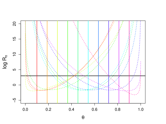
Figure 1: Plots of 95% confidence regions for $\theta_{i}^{*}$ when true values of $\theta_{i}^{*}$ span the interval 0.1 to 0.9 ($n=10$). Here, the $95\%$ CIs are given by the points where the curves for $\log R_{\mathbb{I},n}\left(\bm{\vartheta}_{\mathbb{I}}\right)$ intersect with the horizontal line (black), representing a confidence level of $1-\alpha=0.95$. Each CI can be seen to contain the corresponding true value of $\theta_{i}^{*}$, represented by a vertical line of the same colour as the interval.

3.3.2 Hypothesis testing

Aiming to detect genomic regions that may have differing characteristics between two series, a pertinent question of interest may be considered by testing the hypotheses: $H_{0}$: $\theta_{i1}^{*}=\theta_{i2}^{*}$ vs. $H_{1}$: $\theta_{i1}^{*}\neq\theta_{i2}^{*}$, for every $i\in[n]$ (with $G=2$ series). Then, $\mathbf{D}_{n}=\left(\bm{X}_{i}\right)_{i\in\left[n\right]}$, where $\bm{X}_{i}=(X_{i1},X_{i2})$. From Section 2, the ratio test statistic takes the form

$$T_{\mathbb{I}}\left(\mathbf{D}_{n}\right)=L_{\mathbb{I}}\left(\hat{\gamma}_{\mathbb{I},n},\hat{\beta}_{\mathbb{I},n}\right)/l_{\mathbb{I}}\left(\tilde{\bm{\vartheta}}_{\mathbb{I}}\right)\text{,}$$

where $\hat{\gamma}_{\mathbb{I},n}$ and $\hat{\beta}_{\mathbb{I},n}$ are EB estimators of $\gamma$ and $\beta$, depending only on $\bar{\mathbf{D}}_{\mathbb{I},n}=\mathbf{D}_{n}\backslash\{X_{i1},X_{i2}\}$. With $\tilde{{\vartheta}}_{\mathbb{I}}=\frac{x_{i1}+x_{i2}}{m_{i1}+m_{i2}}=\tilde{\theta}_{i}$, write $l_{\mathbb{I}}\left(\tilde{{\vartheta}}_{\mathbb{I}}\right)=f(x_{i1},x_{i2}|\tilde{\theta}_{i})$, and

$$L_{\mathbb{I}}\left(\hat{\gamma}_{\mathbb{I},n},\hat{\beta}_{\mathbb{I},n}\right) =\int_{\mathbb{T}}f(x_{i1}|\bm{\theta}_{i})f(x_{i2}|\bm{\theta}_{i})\pi(\bm{\theta}_{i};\;\hat{\gamma}_{\mathbb{I},n},\hat{\beta}_{\mathbb{I},n})\text{d}\bm{\theta}_{i}$$

$$=\binom{m_{i1}}{x_{i1}}\binom{m_{i2}}{x_{i2}}\frac{B(x_{i1}+\hat{\gamma}_{\mathbb{I},n},m_{i1}-x_{i1}+\hat{\beta}_{\mathbb{I},n})B(x_{i2}+\hat{\gamma}_{\mathbb{I},n},m_{i2}-x_{i2}+\hat{\beta}_{\mathbb{I},n})}{\left[B(\hat{\gamma}_{\mathbb{I},n},\hat{\beta}_{\mathbb{I},n})\right]^{2}},$$

which gives

$$T_{\mathbb{I}}\left(\mathbf{D}_{n}\right)=\frac{B(x_{i1}+\hat{\gamma}_{\mathbb{I},n},m_{i1}-x_{i1}+\hat{\beta}_{\mathbb{I},n})B(x_{i2}+\hat{\gamma}_{\mathbb{I},n},m_{i2}-x_{i2}+\hat{\beta}_{\mathbb{I},n})}{[B(\hat{\gamma}_{\mathbb{I},n},\hat{\beta}_{\mathbb{I},n})]^{2}\tilde{\theta}_{i}^{x_{i1}+x_{i2}}(1-\tilde{\theta}_{i})^{m_{i1}+m_{i2}-x_{i1}-x_{i2}}},$$

where $\hat{\gamma}_{\mathbb{I},n}$ and $\hat{\beta}_{\mathbb{I},n}$ are calculated in a similar fashion to Section 3.3.1 except that data from both sequences should be used to estimate $\hat{\mu}_{\text{EB}}$ and $\hat{\phi}_{\text{EB}}$, in the sense that

$$\hat{\mu}_{\text{EB}} =\frac{1}{2n-2}\sum_{k\neq i}\sum_{g=1}^{2}\frac{x_{kg}}{m_{kg}},\mbox{ and}$$

$$\hat{\phi}_{\text{EB}} =\left[\frac{\bar{m}V_{xy}}{\hat{\mu}_{\text{EB}}(1-\hat{\mu}_{\text{EB}})}-1\right]\bigg{/}(\bar{m}-1),$$

where

$$\bar{m} =\frac{1}{2n-2}\sum_{k\neq i}\sum_{g=1}^{2}m_{kg},\mbox{ and }$$

$$V_{xy} =\frac{1}{2n-2}\sum_{k\neq i}\sum_{g=1}^{2}\left(\frac{x_{kg}}{m_{kg}}-\hat{\mu}_{\text{EB}}\right)^{2}.$$

In our first simulation, we assessed the performance of the test statistic in terms of the Type I error. Assuming a window size of $n=20$, realized data $(x_{i1},x_{i2})$ ($i\in[n]$), were simulated from independent binomial distributions with $\theta_{i1}^{*}=\theta_{i2}^{*}=\theta_{i}^{*}$ ($i=1,\ldots,n$), with $\theta_{i}^{*}$ ranging between $0.1$ and $0.9$, and $m_{i1},m_{i2}\in\mathbb{N}$ uniformly and independently sampled from the range $[15,40]$. The first panel of Figure 2 shows the calculated test statistic values $T_{\mathbb{I}}\left(\mathbf{D}_{n}\right)$ for the $20$ genomic indices on the logarithmic scale, over 100 independently replicated datasets, with horizontal lines displaying values $\log(1/\alpha)$, for significance levels $\alpha\in\{0.01,0.02,0.05\}$. No points were observed above the line corresponding to $\alpha=0.01$, indicating that the Type I error of the test statistic does not exceed the nominal level. Next, we assessed the power of the test statistic at three levels of significance ($\alpha\in\{0.01,0.02,0.05\}$) and differing effect sizes. For each $i$ ($i\in[n]$), $\theta_{i1}^{*}$ was set to be a value between $0.05$ and $0.95$, and $\theta_{i2}^{*}=\theta_{i1}^{*}+\Delta$, where $0.1<\Delta<0.9$ (with $\theta_{i2}^{*}<1$). A sample of $20$ replicates were simulated under each possible set of values of $(\theta_{1}^{*},\theta_{2}^{*})$. The second panel of Figure 2 shows that the power functions increased rapidly to 1 as the difference $\Delta$ was increased.

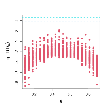
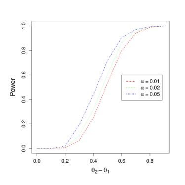
Figure 2: Panel (a): Test statistic for 100 replications of the beta–binomial example under the null hypothesis of equality of proportions. The three horizontal lines correspond to cutoffs according to significance levels of $\alpha=0.05$ (green), $\alpha=0.02$ (blue), and $\alpha=0.01$ (turquoise). Panel (b): Power function over different values of $\Delta=\theta_{2}^{*}-\theta_{1}^{*}$ at three levels of significance: $\alpha\in\{0.01,0.02,0.05\}$.

In our next numerical experiment, we generated data sets of sizes $n\in\{10,100,1000\}$, where realized observations $x_{i1}$, and $x_{i2}$ are simulated from independent binomial distributions with parameters $\theta_{i1}^{*}$ and $\theta_{i2}^{*}$, respectively ($i\in[n]$). For each $i$, $\theta_{i1^{*}}$ was generated from a beta distribution, in turn, with hyperparameters $\bm{\psi}=(\gamma,\beta)\in\{(2,2),(2,5),(5,2)\}$; and $\theta_{i2}^{*}=\theta_{i1}^{*}+\Delta$, where $\Delta\in\{0,0.2,0.5,0.9\}$. We generated 100 instances of data under each setting and assessed the power of the FSEB test statistic through the number of rejections at levels $\alpha\in\{0.0005,0.005,0.05\}$. The results are shown in Table 4.

Similarly to the Poisson–gamma example, it can be seen that the tests reject true null hypotheses at below the nominal sizes $\alpha$, in each case. For each combination of $n$ and $\bm{\psi}$, as $\Delta$ increases, the rejection rate increases, making the tests more powerful as expected, when detecting larger differences between $\theta_{i1}^{*}$ and $\theta_{i2}^{*}$, frequently reaching a power of 1 even when the difference was not maximal. There did not appear to be a clear increase in power with the sample size, within the settings considered. Overall, we may conclude, as previously, that the tests are behaving as expected, although both this example and the Poisson–gamma case show that the tests may be underpowered as they do not achieve the nominal size for any value of $\alpha$.

Table 4: Experimental results for testing the hypothesis $\text{H}_{0}$: $\theta_{i1}^{*}=\theta_{i2}^{*}$ for Beta–binomial count series models. The Rejection proportion columns report the average number of rejections, from 100 test replicates, at levels of significance $\alpha\in\left\{0.05,0.005,0.0005\right\}$.

			Rejection proportion at level $\alpha$
$n$	$\bm{\psi}$	$\Delta$	$0.0005$	$0.005$	$0.05$
10	$(2,2)$	0	0.000	0.000	0.000
		0.2	0.000	0.004	0.039
		0.5	0.305	0.471	0.709
		0.9	0.980	1.000	1.000
	$(2,5)$	0	0.000	0.000	0.000
		0.2	0.000	0.001	0.025
		0.5	0.249	0.464	0.692
		0.9	0.995	1.000	1.000
	$(5,2)$	0	0.000	0.000	0.000
		0.2	0.000	0.006	0.052
		0.5	0.281	0.459	0.690
		0.9	0.993	0.993	1.000
100	$(2,2)$	0	0.000	0.000	0.000
		0.2	0.000	0.004	0.037
		0.5	0.272	0.459	0.700
		0.9	0.996	0.998	1.000
	$(2,5)$	0	0.000	0.000	0.000
		0.2	0.000	0.003	0.032
		0.5	0.267	0.459	0.693
		0.9	0.994	0.999	1.000
	$(5,2)$	0	0.000	0.000	0.000
		0.2	0.000	0.004	0.047
		0.5	0.269	0.459	0.697
		0.9	0.987	0.998	0.999
1000	$(2,2)$	0	0.000	0.000	0.000
		0.2	0.000	0.003	0.031
		0.5	0.280	0.476	0.707
		0.9	0.982	0.992	0.998
	$(2,5)$	0	0.000	0.000	0.000
		0.2	0.000	0.003	0.030
		0.5	0.264	0.459	0.693
		0.9	0.989	0.996	1.000
	$(5,2)$	0	0.000	0.000	0.000
		0.2	0.000	0.005	0.047
		0.5	0.279	0.474	0.706
		0.9	0.986	0.995	0.999

As an additional assessment of how FSEB performs in comparison to other tests in a similar setting, we carried out a number of additional simulation studies, in which FSEB was compared with Fisher’s exact test and a score test, over various settings of $n$, $\bm{\psi}$ and $\Delta$, as well as for different ranges of $m_{i}$ ($i=1\in[n]$). Comparisons were made using the $p$-values as well as false discovery rate (FDR) corrected $p$-values arising from FDR control methods (Wang and Ramdas, 2022), and are presented in the online Supplementary Materials (Tables S1–S8 and Figures S1–S8). It is evident in almost all cases (and especially in case C, which most closely resembles the real life application scenario) that (i) the power levels are very similar across methods, especially as values of $n$, $m_{i}$ ($i\in[n]$) and effect sizes increase, and (ii) in every case, there are some settings in which Fisher’s test and the score test are anti-conservative (even after FDR correction), with their Type I error greatly exceeding the nominal levels of significance, while this never occurs for FSEB, even without FDR correction.

4 Real-data applications

4.1 The Norberg data

We now wish to apply the FSEB CI construction from Section 3.2.1 to produce CIs in a real data application. We shall investigate the Norberg data set from the REBayes package of Koenker and Gu (2017), obtained from Haastrup (2000). These data pertain to group life insurance claims from Norwegian workmen. Here, we have $n=72$ observations $\mathbf{D}_{n}$, containing total number of death claims $X_{i}$, along with covariates $\mathbf{w}_{n}$, where $w_{i}$ is the number of years of exposure, normalized by a factor of 344, for $i\in\left[n\right]$. Here each $i$ is an individual occupation group.

To analyze the data, we use the Poisson–gamma model and estimate the generative parameters $\bm{\vartheta}_{n}^{*}$ using estimates of form (13). Here, each $\theta_{i}^{*}$ can be interpreted as an unobserved multiplicative occupation specific risk factor that influences the number of claims made within occupation group $i$. To obtain individually-valid $95\%$ CIs for each of the $n$ estimates, we then apply the method from Section 3.2.1. We present both the estimated risk factors and their CIs in Figure 3.

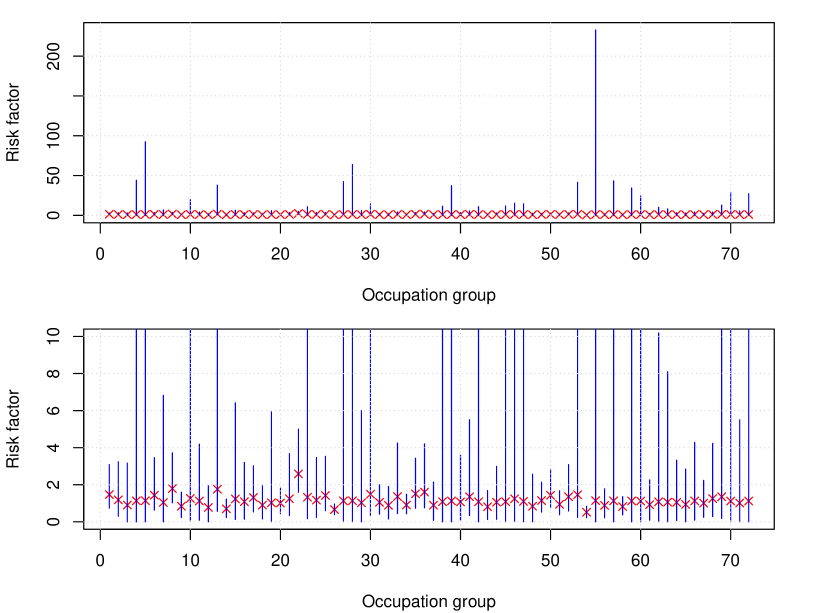
Figure 3: Estimates of risk factors $\bm{\vartheta}_{n}^{*}$ for the Norberg data set along with associated $95\%$ CIs. The estimated risk factor for each occupation group is depicted as a cross and the associate (individually-valid) CI is depicted as a line. The top plot displays the CIs at their entire lengths, whereas the bottom plot displays only the risk factor range between 0 and 10.

From Figure 3, we notice that most of the estimates of $\bm{\vartheta}_{n}^{*}$ are between zero and two, with the exception of occupation group $i=22$, which has an estimated risk factor of $\theta_{22}^{*}=2.59$. Although the risk factors are all quite small, the associated CIs can become very large, as can be seen in the top plot. This is due to the conservative nature of the CI constructions that we have already observed from Section 3.1.

We observe that wider CIs were associated with observations where $X_{i}=0$, with $w_{i}$ being small. In particular, the largest CI, occurring for $i=55$, has response $X_{55}=0$ and the smallest covariate value in the data set: $w_{55}=4.45$. The next largest CI occurs for $i=5$ and also corresponds to a response $X_{5}=0$ and the second smallest covariate value $w_{5}=11.30$.

However, upon observation of the bottom plot, we see that although some of the CIs are too wide to be meaningful, there are still numerous meaningful CIs that provide confidence regarding the lower limits as well as upper limits of the underlying risk factors. In particular, we observe that the CIs for occupation groups $i=26$ and $i=54$ are remarkably narrow and precise. Of course, the preceding inferential observations are only valid when considering each of the $n$ CIs, individually, and under the assumption that we had chosen to draw inference regarding the corresponding parameter of the CI, before any data are observed.

If we wish to draw inference regarding all $n$ elements of $\bm{\vartheta}_{n}^{*}$, simultaneously, then we should instead construct a $100\left(1-\alpha\right)\%$ simultaneous confidence set $\bar{\mathcal{C}}^{\alpha}\left(\mathbf{D}_{n}\right)$, with the property that

$$\text{Pr}_{\bm{\vartheta}_{n}^{*}}\left[\bm{\vartheta}_{n}^{*}\in\bar{\mathcal{C}}^{\alpha}\left(\mathbf{D}_{n}\right)\right]\geq 1-\alpha\text{.}$$

Using Bonferroni’s inequality, we can take $\bar{\mathcal{C}}^{\alpha}\left(\mathbf{D}_{n}\right)$ to be the Cartesian product of the individual $100\left(1-\alpha/n\right)\%$ (adjusted) CI for each parameter $\theta_{i}^{*}$:

$$\bar{\mathcal{C}}^{\alpha}\left(\mathbf{D}_{n}\right)=\prod_{i=1}^{n}\mathcal{C}_{i}^{\alpha/n}\left(\mathbf{D}_{n}\right)\text{.}$$

Using the $\alpha=0.05$, we obtain the $95\%$ simultaneous confidence set that appears in Figure 4. We observe that the simultaneous confidence set now permits us to draw useful inference regarding multiple parameters, at the same time. For example, inspecting the $n$ adjusted CIs, we observe that the occupations corresponding to indices $i\in\left\{8,22,50\right\}$ all have lower bounds above $0.5$. Thus, interpreting these indices specifically, we can say that each of the three adjusted confidence intervals, which yield the inference that the risk factors $\theta_{i}^{*}>0.5$ for $i\in\left\{8,22,50\right\}$, contains the parameter $\theta_{i}^{*}$ with probability $0.95$, under repeated sampling.

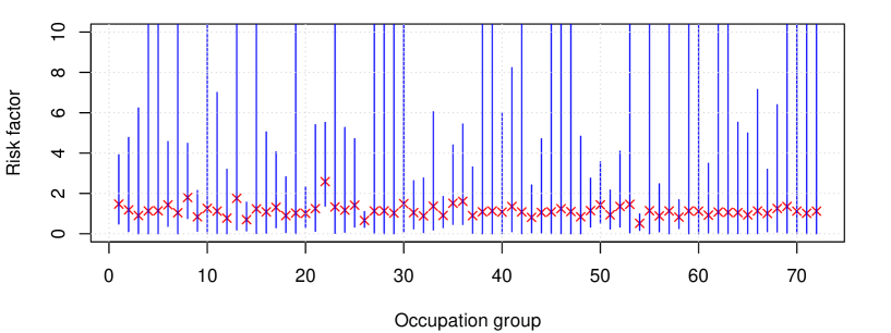
Figure 4: Estimates of risk factors $\bm{\vartheta}_{n}^{*}$ for the Norberg data set along with the associated simultaneous $95\%$ confidence set. The estimated risk factors for each occupation group is depicted as a cross and the simultaneous confidence set can be constructed via the cartesian product of the adjusted CIs, depicted as lines. The plot is focused on the risk factor range between 0 and 10.

Since our individual CI and adjusted CI constructions are $e$-CIs, one can alternatively approach the problem of drawing simultaneously valid inference via the false coverage rate (FCR) controlling techniques of Xu et al. (2022). Using again the parameters $\theta_{i}^{*}$ corresponding to $i\in\left\{8,22,50\right\}$, as an example, we can use Theorem 2 of Xu et al. (2022) to make the statement that the three adjusted CIs $\mathcal{C}_{i}^{3\alpha/n}\left(\mathbf{D}_{n}\right)$, for $i\in\left\{8,22,50\right\}$, can be interpreted at the FCR controlled level $\alpha\in(0,1)$, in the sense that

$$\text{E}_{\bm{\vartheta}_{\mathbb{I}\left(\mathbf{D}_{n}\right)}^{*}}\left[\frac{\sum_{i\in\mathbb{I}}\left\llbracket\theta_{i}^{*}\notin\mathcal{C}_{i}^{\left|\mathbb{I}\left(\mathbf{D}_{n}\right)\right|\alpha/n}\left(\mathbf{D}_{n}\right)\right\rrbracket}{\max\left\{1,\left|\mathbb{I}\left(\mathbf{D}_{n}\right)\right|\right\}}\right]\leq\alpha\text{,}$$

where $\mathbb{I}\left(\mathbf{D}_{n}\right)$ is a data-dependent subset of parameter indices. In particular, we observe the realization $\left\{8,22,50\right\}$ of $\mathbb{I}\left(\mathbf{D}_{n}\right)$, corresponding to the data-dependent rule of selecting indices with adjusted CIs $\mathcal{C}_{i}^{\alpha/n}\left(\mathbf{D}_{n}\right)$ with lower bounds greater than $0.5$. Here, $\left\llbracket\mathsf{A}\right\rrbracket=1$ if statement $\mathsf{A}$ is true and $0$, otherwise.

Clearly, controlling the FCR at level $\alpha$ yields narrower CIs for each of our the three assessed parameters than does the more blunt simultaneous confidence set approach. In particular, the $95\%$ simultaneous adjusted CIs obtained via Bonferroni’s inequality are $\left(0.775,4.485\right)$, $\left(1.375,5.520\right)$, and $\left(0.505,3.565\right)$, and the $0.05$ level FCR controlled adjusted CIs are $\left(0.810,4.300\right)$, $\left(1.430,5.390\right)$, and $\left(0.555,3.390\right)$, for the parameters $\theta_{i}^{*}$ corresponding to the respective parameters $i\in\left\{8,22,50\right\}$. Overall, these are positive results as we do not know of another general method for generating CIs in this EB setting, whether individually or jointly.

4.2 Differential methylation detection in bisulphite sequencing data

DNA methylation is a chemical modification of DNA caused by the addition of a methyl ($CH_{3}$-) group to a DNA nucleotide – usually a C that is followed by a G – called a CpG site, which is an important factor in controlling gene expression over the human genome. Detecting differences in the methylation patterns between normal and ageing cells can shed light on the complex biological processes underlying human ageing, and hence has been an important scientific problem over the last decade (Smith and Meissner, 2013). Methylation patterns can be detected using high-throughput bisulphite sequencing experiments (Krueger et al., 2012), in which data are generated in the form of sequences of numbers of methylated cytosines, $x_{ig}$, among the total counts of cytosines, $m_{ig}$, for $n$ CpG sites on a genome $(i\in[n])$, for $G$ groups of cell types $g\in[G]$. Often, there are $G=2$ groups, as in our example that follows, for which the question of interest is to detect regions of differential methylation in the DNA of normal and ageing cells. Based on the setup above, a set of bisulphite sequencing data from an experiment with $G$ groups might be considered as $G$ series of (possibly correlated) observations from non-identical binomial distributions. The degree of dependence between adjacent CpG sites typically depends on the genomic distance between these loci, but since these are often separated by hundreds of bases, for the moment it is assumed that this correlation is negligible and is not incorporated into our model.

4.2.1 Application to Methylation data from Human chromosome 21

We evaluated the test statistic $T_{\mathbb{I}}\left(\mathbf{D}_{n}\right)$ over a paired segment of methylation data from normal and ageing cells, from $100,000$ CpG sites on human chromosome 21 (Cruickshanks et al., 2013). After data cleaning and filtering (to remove sites with too low or too high degrees of experimental coverage, that can introduce errors), $58,361$ sites remained for analysis. Figure 5 shows the predicted demarcation of the data into differentially and non-differentially methylated sites over the entire region, at three cutoff levels of significance, overlaid with a moving average using a window size of 10 sites. It was observed that large values of the test statistic were often found in grouped clusters, which would be biologically meaningful, as loss of methylation in ageing cells is more likely to be highly region-specific, rather than randomly scattered over the genome. The overall rejection rates for the FSEB procedure corresponding to significance levels of $\alpha=0.0005,0.05,0.02$ and $0.01$ were found to be $0.0012$, $0.0154$, $0.0092$, and $0.0064$, respectively.

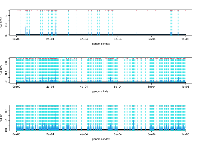
Figure 5: FSEB test statistics over a segment of methylation data. The panels show the demarcation of loci into differentially methylated (coded as “$1$”) and non-differentially methylated sites (coded as “$0$”) with an overlay of a moving average with a window size of 10 CpG sites, at significance level cutoffs of $0.0005$, $0.005$, and $0.05$.

As a comparison to other methods for detecting differential methylation, we also applied site-by-site Fisher tests and score tests as implemented for bisulphite sequencing data in the R Bioconductor package DMRcaller (Catoni et al., 2018). For purposes of comparison, we used two significance level cutoffs of $0.05$ and $0.0005$ for our FSEB test statistic, along with the same cutoffs subject to a Benjamini–Hochberg FDR correction for the other two testing methods. Figure 6 shows the comparison between the calculated site-specific $p$-values of the Fisher and score tests with the calculated FSEB test statistic (all on the logarithmic scale) over the entire genomic segment, which indicates a remarkable degree of overlap in the regions of differential methylation. There are, however, significant differences as well, in both the numbers of differential methylation calls and their location. In particular, the FSEB test statistic appeared to have stronger evidence for differential methylation in two regions, one on the left side of the figure, and one towards the centre. The Fisher test, being the most conservative, almost missed this central region (gave a very weak signal), while the score test gave a very high proportion of differential methylation calls compared to both other methods – however, the results from the score test may not be as reliable as many cells contained small numbers of counts which may render the test assumptions invalid. Table 5 gives a summary of the overlap and differences of the results from the different methods at two levels of significance, indicating that with FDR corrections, the Fisher test appears to be the most conservative, the score test the least conservative, and the FSEB procedure in-between the two. We also calculated, for each pair of methods, the proportion of matching calls, defined as the ratio of the number of sites predicted by both methods as either differentially methylated, or non-differentially methylated, to the total number of sites. These proportions indicated a high degree of concordance, especially between FSEB and Fisher tests, with the score test showing the least degree of concordance at both levels of significance. As expected, the degree of concordance decreased with an increase in $\alpha$, but only slightly so, between the FDR-corrected Fisher test and FSEB.

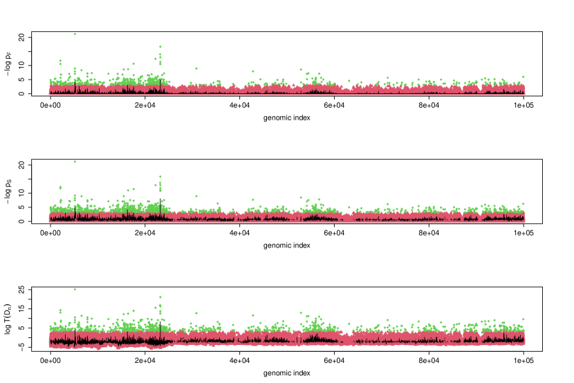
Figure 6: Results of three testing procedures to detect sites of differential methylation over a segment of methylation data. The first two panels show the negative logarithms of the FDR-corrected $p$-values for the (i) Fisher test ($-\log p_{F}$) and (ii) score test ($-\log p_{S}$), while the third panel shows the logarithm of the FSEB test statistic ($\log T(D_{n})$). The black curve in each plot corresponds to a moving average with a window size of 10. The points are coloured by differential methylation state call: green if differentially methylated, and red if not, at test size $0.05$.

Table 5: Comparison of differential methylation calling results between different methods: (i) FSEB (ii) Fisher tests with FDR-adjusted $p$-values (FF) (iii) Fisher tests, unadjusted (F) (iv) score tests with FDR-adjusted $p$-values (SF) and (v) score tests, unadjusted (S). The upper table gives the proportions of sites called to be differentially expressed under the tests of sizes $\alpha\in\{0.0005,0.05\}$. The lower table gives the proportion of overlaps between differential methylation calls from each pair of methods at a fixed level $\alpha\in\{0.0005,0.05\}$.

	Proportion of rejections at level
	$\alpha=0.0005$	$\alpha=0.05$
FSEB	0.0012	0.0154
FF	0.0003	0.0097
F	0.0098	0.1102
SF	0.1333	0.1528
S	0.1457	0.2926

	Proportion of overlap in matching calls at level
	$\alpha=0.0005$					$\alpha=0.05$
Method	FF	F	SF	S	Method	FF	F	SF	S
FSEB	0.999	0.991	0.866	0.856	FSEB	0.992	0.905	0.860	0.723
FF		0.991	0.867	0.855	FF		0.900	0.857	0.717
F			0.858	0.864	SF			0.777	0.818
SF				0.988	S				0.860

5 Conclusion

EB is a powerful and popular paradigm for conducting parametric inference in situations where the DGP can be assumed to possess a hierarchical structure. Over the years, general frameworks for point estimation have been developed for EB, such as via the shrinkage estimators of Serdobolskii (2008) or the various method of moments and likelihood-based methods described in Maritz and Lwin (1989, Sec. 3). Contrastingly, the construction of interval estimators and hypothesis tests for EB parameters rely primarily on bespoke derivations and analysis of the specific models under investigation.

In this paper, we have adapted the general universal inference framework for finite sample valid interval estimation and hypothesis testing of Wasserman et al. (2020) to construct a general framework within the EB setting, which we refer to as the FSEB technique. In Section 2, we proved that these FSEB techniques generate valid confidence sets and hypothesis tests of the correct size. In Section 3, we demonstrated via numerical simulations, that the FSEB methods can be used in well-studied synthetic scenarios. There, we highlight that the methods can generate meaningful inference for realistic DGPs. This point is further elaborated in Section 4, where we also showed that our FSEB approach can be usefully applied to draw inference from real world data, in the contexts of insurance risk and the bioinformatics study of DNA methylation.

We note that although our framework is general, due to it being Markov inequality-based, it shares the same general criticism that may be laid upon other universal inference methods, which is that the confidence sets and hypothesis tests can often be conservative, in the sense that the nominal confidence level or size is not achieved. The lack of power due to the looseness of Markov’s inequality was first mentioned and discussed in Wasserman et al. (2020), where it is also pointed out that, in the universal inference setting, the logarithm of the analogous ratio statistics to (6) have tail probabilities that scale, in $\alpha$, like those of $\chi^{2}$ statistics. The conservativeness of universal inference constructions is further discussed in the works of Dunn et al. (2021), Tse and Davison (2022), and Strieder and Drton (2022), where the topic is thoroughly explored via simulations and theoretical results regarding some classes of sufficiently regular problems. We observe this phenomenon in the comparisons in Sections 3.1 (and further expanded in the Supplementary Materials). We also explored subsampling-based tests within the FSEB framework, along the lines proposed by Dunn et al. (2021), which led to very minor increases in power in some cases with small sample sizes without affecting the Type I error. With such an outcome not entirely discernible from sampling error, and with the substantial increase to computational cost, it does not seem worthwhile to employ the subsampling-based approach here. A possible reason for the lack improvement in power observed, despite subsampling, can be attributed to the fact that the sets $\mathbb{I}$, and their complements, are not exchangeable; since the indices fundamentally define the hypotheses and parameters of interest.

However, we note that since the methodology falls within the $e$-value framework, it also inherits desirable properties, such as the ability to combine test statistics by averaging (Vovk and Wang, 2021), and the ability to more-powerfully conduct false discovery rate control when tests are arbitrarily dependent (Wang and Ramdas, 2022).

Overall, we believe that FSEB techniques can be usefully incorporated into any EB-based inference setting, especially when no other interval estimators or tests are already available, and are a useful addition to the statistical tool set. Although a method that is based on the careful analysis of the particular setting is always preferable in terms of exploiting the problem specific properties in order to generate powerful tests and tight intervals, FSEB methods can always be used in cases where such careful analyses may be mathematically difficult or overly time consuming.

References

- Ahmed and Reid [2001] S E Ahmed and N Reid, editors. Empirical Bayes and Likelihood Inference. Springer, New York, 2001.
- Bickel [2020] D R Bickel. Genomics Data Analysis: False Discovery Rates and Empirical Bayes Methods. CRC Press, Boca Raton, 2020.
- Casella and Hwang [1983] G Casella and J T Hwang. Empirical Bayes confidence sets for the mean of a multivariate normal distribution. Journal of the American Statistical Association, 78:688–698, 1983.
- Catoni et al. [2018] M Catoni, J M Tsang, A P Greco, and N R Zabet. DMRcaller: a versatile R/Bioconductor package for detection and visualization of differentially methylated regions in CpG and non-CpG contexts. Nucleic Acids Research, 46:e114, 2018.
- Cruickshanks et al. [2013] H A Cruickshanks, T McBryan, D M Nelson, N D Vanderkraats, P P Shah, J van Tuyn, T S Rai, C Brock, G Donahue, D S Dunican, M E Drotar, R R Meehan, J R Edwards, S L Berger, and P D Adams. Senescent cells harbour features of the cancer epigenome. Nature Cell Biology, 15:1495–1506, 2013.
- Datta et al. [2002] G S Datta, M Ghosh, D D Smith, and P Lahiri. On an asymptotic theory of conditional and unconditional coverage probabilities of empirical Bayes confidence intervals. Scandinavian Journal of Statistics, 29:139–152, 2002.
- Dunn et al. [2021] R Dunn, A Ramdas, S Balakrishnan, and L Wasserman. Gaussian universal likelihood ratio testing. arXiv:2104.14676, 2021.
- Efron [2010] B Efron. Large-scale Inference. Cambridge University Press, Cambridge, 2010.
- Grunwald et al. [2020] P Grunwald, R de Heide, and W M Koolen. Safe testing. In Information Theory and Applications Workshop (ITA), 2020.
- Haastrup [2000] S Haastrup. Comparison of some Bayesian analyses of heterogeneity in group life insurance. Scandinavian Actuarial Journal, 2000:2–16, 2000.
- Hardcastle and Kelly [2013] T J Hardcastle and K A Kelly. Empirical Bayesian analysis of paired high-throughput sequencing data with a beta-binomial distribution. BMC Bioinformatics, 14:135, 2013.
- Hwang and Zhao [2013] J T G Hwang and Z Zhao. Empirical Bayes confidence intervals for selected parameters in high-dimensional data. Journal of the American Statistical Association, 108:607–618, 2013.
- Hwang et al. [2009] J T G Hwang, J Qiu, and Z Zhao. Empirical Bayes confidence intervals shrinking both means and variances. Journal of the Royal Statistical Society B, 71:265–285, 2009.
- Johnstone and Silverman [2005] I M Johnstone and B W Silverman. EbayesThresh: R programs for empirical Bayes thresholding. Journal of Statistical Software, 12:1–38, 2005.
- Kaufmann and Koolen [2018] E Kaufmann and W M Koolen. Mixture martingales revisited with applications to sequential tests and confidence intervals. arXiv:1811.11419v1, 2018.
- Koenker and Gu [2017] R Koenker and J Gu. REBayes: Empirical Bayes mixture methods in R. Journal of Statistical Software, 82:1–26, 2017.
- Krueger et al. [2012] F Krueger, B Kreck, A Franke, and S R Andrews. DNA methylome analysis using short bisulfite sequencing data. Nature Methods, 9:145–151, 2012.
- Laird and Louis [1987] N M Laird and T A Louis. Empirical Bayes confidence intervals based on bootstrap samples. Journal of the American Statistical Association, 82:739–750, 1987.
- Leng et al. [2013] N Leng, J A Dawson, J A Thomson, V Ruotti, A I Rissman, B M G Smits, J D Haag, M N Gould, R M Stewart, and C Kendziorski. EBSeq: an empirical Bayes hierarchical model for inference in RNA-seq experiments. Bioinformatics, 29:1035–1043, 2013.
- Maritz and Lwin [1989] J S Maritz and T Lwin. Empirical Bayes Methods. CRC Press, Boca Raton, 1989.
- Morris [1983a] C N Morris. Parametric empirical Bayes inference: theory and applications. Journal of the American Statistical Association, 78:47–55, 1983a.
- Morris [1983b] C N Morris. Parametric empirical bayes confidence intervals. In Scientific inference, data analysis, and robustness. Elsevier, 1983b.
- Narasimhan and Efron [2020] B Narasimhan and B Efron. deconvolveR: a G-modeling program for deconvolution and empirical Bayes estimation. Journal of Statistical Software, 94:1–20, 2020.
- Norberg [1989] R Norberg. Experience rating in group life insurance. Scandinavian Actuarial Journal, 1989:194–224, 1989.
- Serdobolskii [2008] V I Serdobolskii. Multiparametric Statistics. Elsevier, Amsterdam, 2008.
- Shafer [2021] G Shafer. Testing by betting: a strategy for statistical and scientific communication. Journal of the Royal Statistical Society B, 184:407–431, 2021.
- Smith and Meissner [2013] Z D Smith and A Meissner. DNA methylation: roles in mammalian development. Nature Reviews Genetics, 14:204–220, 2013.
- Stein [1956] C Stein. Inadmissibility of the usual estimator for the mean of a multivariate normal distribution. In Berkeley Symposium on Mathematical Statistics and Probability, 1956.
- Strieder and Drton [2022] D Strieder and M Drton. On the choice of the splitting ratio for the split likelihood ratio test. arXiv:2203.06748, 2022.
- Tai and Speed [2006] Y C Tai and T P Speed. A multivariate empirical Bayes statistic for replicated microarray time course data. Annals of Statistics, 34:2387–2412, 2006.
- Tse and Davison [2022] T Tse and A C Davison. A note on universal inference. Stat, to appear, 2022.
- Vovk [2007] V Vovk. Strong confidence intervals for autoregression. arXiv:0707.0660v1, 2007.
- Vovk and Wang [2021] V Vovk and R Wang. E-values: calibration, combination, and applications. Annals of Statistics, 49:1736–1754, 2021.
- Wang and Ramdas [2022] R Wang and A Ramdas. False discovery rate control with e-values. Journal of the Royal Statistical Society B, 84:822–852, 2022.
- Wasserman et al. [2020] L Wasserman, A Ramdas, and S Balakrishnan. Universal inference. Proceedings of the National Academy of Sciences, 117:16880–16890, 2020.
- Xu et al. [2022] Z Xu, R Wang, and A Ramdas. Post-selection inference for e-value based confidence intervals. arXiv:2203.12572, 2022.
- Yoshimori and Lahiri [2014] M Yoshimori and P Lahiri. A second-order efficient empirical Bayes confidence interval. Annals of Statistics, 42:1233–1261, 2014.