Spatial Curvature from Super-Hubble Cosmological Fluctuations

Abstract

We revisit how super-Hubble cosmological fluctuations induce, at any time in the cosmic history, a non-vanishing spatial curvature of the local background metric. The random nature of these fluctuations promotes the curvature density parameter to a stochastic quantity for which we derive novel non-perturbative expressions for its mean, variance, higher moments and full probability distribution. For scale-invariant Gaussian perturbations, such as those favored by cosmological observations, we find that the most probable value for the curvature density parameter $\Omega_{\mathrm{K}}$ today is $-10^{-9}$, and that its mean is $+10^{-9}$, both being overwhelmed by a standard deviation of order of $10^{-5}$. We then discuss how these numbers would be affected by the presence of large super-Hubble non-Gaussianities, or if inflation lasted for a very long time. In particular, we find that substantial values of $\Omega_{\mathrm{K}}$ are obtained if inflation lasts for more than a billion $e$-folds.

I Introduction

Cosmic structures in the Universe are understood to be seeded by some pre-existing super-Hubble cosmological fluctuations. Their gravitational collapse starts when their size becomes smaller than the Hubble radius, an inevitable outcome in any decelerating Friedmann-Lemaître spacetime. Observational evidence of this mechanism is present in the Cosmic Microwave Background (CMB) data by the correlation patterns associated with the polarization and temperature angular power spectra Hu et al. (1997); Aghanim et al. (2020), as well as in the statistics of the large-scale structures observed at lower redshifts Fonseca et al. (2015); Tutusaus et al. (2020).

Cosmic Inflation, an early era of accelerated cosmic expansion, is the prime candidate to explain the origin of the super-Hubble fluctuations. They are of quantum origin, stretched to length scales much larger than the Hubble radius during inflation Starobinsky (1979, 1980); Guth (1981); Linde (1982); Albrecht and Steinhardt (1982); Linde (1983); Mukhanov and Chibisov (1981, 1982); Starobinsky (1982); Guth and Pi (1982); Hawking (1982); Bardeen et al. (1983). At the same time, inflation smooths out any pre-existing inhomogeneity, and one of the historical motivations for Cosmic Inflation is that the spatial curvature of spacetime, $\Omega_{\mathrm{K}}$, should be exponentially small at the end of inflation (at most $e^{-60}$). This prediction is compatible with the current bound $|\Omega_{\mathrm{K}_{0}}|<3\times 10^{-3}$ today, coming from the Planck CMB data and Baryon Acoustic Oscillations (BAO) measurements.

Intuitively, the existence, today, of Hubble-sized curvature fluctuations suggests that these could be confused with a small non-vanishing spatial curvature of the local background metric. In particular, these modes are expected to induce a limitation on our ability to measure very small values of the curvature density parameter Waterhouse and Zibin (2008); Buchert and Carfora (2008); Vardanyan et al. (2009); Leonard et al. (2016); Anselmi et al. (2023). More than being a nuisance, we will show that super-Hubble (hence, “conserved”) fluctuations do create spatial curvature.

In order to deal with fluctuations over a background metric when both are intertwined, we can start from the inhomogeneous metric proposed in Refs. Salopek and Bond (1990); Creminelli and Zaldarriaga (2004); Kolb et al. (2005a); Lyth et al. (2005):

$$\differential s^{2}=-\differential\tau^{2}+a^{2}(\tau)e^{2\zeta(\tau,{\bf\it x})}\delta_{ij}\differential x^{i}\differential x^{j}.$$ (1)

This metric is not fully general, as inhomogeneities are all contained in one scalar function $\zeta$. However, as discussed in Refs. Salopek and Bond (1990); Creminelli and Zaldarriaga (2004); Kolb et al. (2005a); Lyth et al. (2005), this is the most generic metric in the absence of vector- and tensor-type inhomogeneities, and in the gauge where fixed time slices have uniform energy density and fixed spatial worldlines are comoving with matter. At super-Hubble scales, this reduces to the synchronous gauge supplemented by some additional conditions that fix it uniquely. The quantity $\zeta(\tau,{\bf\it x})$ can be shown to be “conserved” at large distances. As such, it provides a non-linear generalization of the constant-energy-density curvature perturbation Rigopoulos and Shellard (2005); Langlois and Vernizzi (2005).

Historically, this metric has been intensively discussed in the attempts to explain the acceleration of the Universe by the backreaction of super-Hubble inhomogeneities Kolb et al. (2005b); Barausse et al. (2005). But, as realized soon after Hirata and Seljak (2005); Kolb et al. (2006); Geshnizjani et al. (2005), the effects of super-Hubble fluctuations onto the background evolution are to modify the spatial curvature. Let us notice that, on top of the background evolution, other observable signatures are possible Grishchuk and Zeldovich (1978); Garcia-Bellido et al. (1995); Erickcek et al. (2008). To our knowledge, the only works having addressed how super-Hubble modes affect the spatial curvature are Refs. Brandenberger and Lam (2004); Geshnizjani et al. (2005); Kleban and Schillo (2012), based, however, on perturbative gradient expansions or linear perturbation theory only. When the non-perturbative terms of our derivation can be neglected, we recover some of their results.

The paper is organized as follows. In Section II, we derive an exact expression for the curvature density parameter $\Omega_{\mathrm{K}}$ in terms of the non-linear curvature perturbation $\zeta$. This promotes $\Omega_{\mathrm{K}}$ to a stochastic quantity, and in Section III we calculate its moments as well as its probability density function, assuming Gaussian statistics for $\zeta$. Finally, we conclude by discussing how the statistics of the curvature density parameter is modified in the presence of non-Gaussian super-Hubble fluctuations or if inflation lasted for a very long time.

II Curvature density parameter

When spatial curvature is included, the Friedmann-Lemaître-Robertson-Walker (FLRW) line element reads

$$\differential s^{2}=-\differential\tau^{2}+a^{2}(\tau)\frac{\delta_{ij}\differential x^{i}\differential x^{j}}{\left(1+\frac{K}{4}\delta_{mn}x^{m}x^{n}\right)^{2}}\,,$$ (2)

where $K$ is a constant, and its Ricci scalar is given by

$$R=6\frac{\dot{a}^{2}}{a^{2}}+6\frac{\ddot{a}}{a}+\frac{6}{a^{2}}K.$$ (3)

The metric (1) can be viewed as an inhomogeneous generalization of a flat, i.e., $K=0$, FLRW spacetime having a space-dependent scale factor

$$b(\tau,{\bf\it x})\equiv a(\tau)e^{\zeta(\tau,{\bf\it x})},$$ (4)

from which one can derive the Ricci scalar

$$R=6\dfrac{\dot{b}^{2}}{b^{2}}+6\dfrac{\ddot{b}}{b}+2\dfrac{(\vnabla b)^{2}}{b^{4}}-4\dfrac{\Delta b}{b^{3}}\,.$$ (5)

We now split $\zeta(\tau,{\bf\it x})=\xi({\bf\it x})+\zeta_{\mathrm{s}}(\tau,{\bf\it x})$ into a conserved part $\xi$ (super-Hubble) and time-dependent fluctuations $\zeta_{\mathrm{s}}$ (sub-Hubble). Expanding in the (presumably small) short-length part, one has

$$b(\tau,{\bf\it x})=a(\tau)e^{\xi({\bf\it x})}\left[1+\zeta_{\mathrm{s}}(\tau,{\bf\it x})+\cdots\right],$$ (6)

and upon defining

$$\tilde{a}(\tau,{\bf\it x})=a(\tau)e^{\xi({\bf\it x})}$$ (7)

one is led to

$$R=6\dfrac{\dot{\tilde{a}}^{2}}{\tilde{a}^{2}}+6\dfrac{\ddot{\tilde{a}}}{\tilde{a}}+\dfrac{6}{\tilde{a}^{2}}\left[-\dfrac{2}{3}\Delta\xi-\dfrac{1}{3}\left(\vnabla\xi\right)^{2}\right]+\cdots.$$ (8)

The omitted terms in this expression are the ones appearing in the linear theory of cosmological perturbations, in the synchronous gauge, completed by all possible non-linear corrections involving powers of $\zeta_{\mathrm{s}}(\tau,{\bf\it x})$ and products with $\tilde{a}(\tau,{\bf\it x})$ Carrilho and Malik (2016). The mixed terms involving both $\tilde{a}(\tau,{\bf\it x})$ and powers of $\zeta_{\mathrm{s}}(\tau,{\bf\it x})$ were precisely the ones discussed in the early works on backreaction and are non-observable Geshnizjani et al. (2005); Hirata and Seljak (2005); Kolb et al. (2006). As can be checked in Eq. 8, the terms we have kept are invariant by a constant shift of $\xi({\bf\it x})$, up to a redefinition of $a(\tau)$.

Since $\xi({\bf\it x})$ varies on super-Hubble length scales only, so does $\tilde{a}(\tau,{\bf\it x})$; hence, any observer will identify $\tilde{a}(\tau,{\bf\it x})$ as the FLRW scale factor of their local Hubble patch. Let us notice that, in the gauge we work in, the Hubble radius is the same for all observers, since Geshnizjani and Brandenberger (2002); Matarrese et al. (2004); Kolb et al. (2005a)

$$\tilde{H}\equiv\dfrac{\dot{\tilde{a}}}{\tilde{a}}=\dfrac{\dot{a}}{a}=H,$$ (9)

which does not depend on ${\bf\it x}$. An important remark is that Eqs. 3 and 8 coincide upon identifying

$$K=-\dfrac{2}{3}\Delta\xi-\dfrac{1}{3}\left(\vnabla\xi\right)^{2},$$ (10)

which is indeed constant, since $\xi$ is conserved, and whose measurable curvature density parameter reads

$$\Omega_{\mathrm{K}}=-\dfrac{K}{\tilde{a}^{2}\tilde{H}^{2}}=-\dfrac{Ke^{-2\xi}}{a^{2}H^{2}}\,.$$ (11)

Let us stress that Eq. (10) is exact in the sense that all the terms omitted involve $\zeta_{\mathrm{s}}(\tau,{\bf\it x})$; hence, they are time-dependent and cannot be absorbed in $K$. Equation (10) makes also explicit that only gradients of super-Hubble inhomogeneities have a non-trivial effect.

III Statistics

Current cosmological measurements Akrami et al. (2020a) imply that $\zeta$ has Gaussian statistics and can, thus, be treated as a random Gaussian field, with vanishing mean and higher-point correlation functions entirely determined by the power spectrum

$$\expectationvalue{\zeta({\bf\it k})\zeta({\bf\it k}^{\prime})}=\left(2\pi\right)^{3}\delta({\bf\it k}+{\bf\it k}^{\prime})P_{\zeta}(k).$$ (12)

This is also in agreement with the most favored inflationary scenarios, where the mean values are identified with vacuum expectation values of quantum operators in the Bunch-Davis vacuum. Later on, we will also use the spherical power spectrum $\mathcal{P}_{\zeta}(k)$ defined by

$$\mathcal{P}_{\zeta}(k)=\dfrac{k^{3}}{2\pi^{2}}P_{\zeta}(k)\simeq\mathcal{P}_{*},$$ (13)

where the last approximation holds for a scale-invariant power spectrum.

From Eqs. 10 and 11, $\Omega_{\mathrm{K}}$ can, therefore, also be seen as a stochastic quantity, though its non-linear dependence on $\xi$, and, thus, on $\zeta$, implies that it does not feature Gaussian statistics. In particular, its expectation value does not necessarily vanish.

Let us make the decomposition $\zeta(\tau,{\bf\it x})=\xi({\bf\it x})+\zeta_{\mathrm{s}}(\tau,{\bf\it x})$ explicit in Fourier space:

$$\zeta(\tau,{\bf\it x}) =\dfrac{1}{\left(2\pi\right)^{3}}\int\differential^{3}{\bf\it k}\,\mathrm{\Theta}\!\left(k_{\sigma}-k\right)\zeta({\bf\it k})e^{i{\bf\it k}\dotproduct{\bf\it x}}$$ (14)

$$+\dfrac{1}{\left(2\pi\right)^{3}}\int\differential^{3}{\bf\it k}\mathrm{\Theta}\!\left(k-k_{\sigma}\right)\zeta(\tau,{\bf\it k})e^{i{\bf\it k}\dotproduct{\bf\it x}},$$

where we have introduced a wave number $k_{\sigma}$ below which all Fourier modes $\zeta(\tau,k<k_{\sigma})=\zeta(k)$ can be approximated as time independent. Based on the theory of cosmological perturbations, and its generalizations Rigopoulos and Shellard (2005); Langlois and Vernizzi (2005), this wave number is at most of the order of the conformal Hubble parameter at the observer’s time, say, $\tau_{0}$; namely, $k_{\sigma}\lesssim\tilde{a}(\tau_{0})\tilde{H}(\tau_{0})$. Let us remark the presence of $\tilde{a}(\tau_{0},{\bf\it x})$, instead of $a(\tau_{0})$, in this expression. A priori, this would induce an extra dependence on ${\bf\it x}$ in Eq. 14, where one should write $k_{\sigma}({\bf\it x})$. In order to circumvent this issue, we can, for now, simply choose the cutoff $k_{\sigma}$ to be sufficiently small such that it encompasses all possible spatial modulations of $\tilde{a}(\tau_{0},{\bf\it x})$. In other words, we define

$$k_{\sigma}\equiv\sigma a_{{0}}H_{{0}}\,,$$ (15)

where, in principle, $\sigma<e^{{\min}_{{\bf\it x}}(\xi)}$. As such, we can identify the conserved quantity with

$$\xi({\bf\it x})=\dfrac{1}{\left(2\pi\right)^{3}}\int\differential^{3}{\bf\it k}\,\mathrm{\Theta}\!\left(k_{\sigma}-k\right)\zeta({\bf\it k})e^{i{\bf\it k}\dotproduct{\bf\it x}}\,.$$ (16)

Let us remark that $\sigma$ also quantifies the possible ambiguities in separating the background, made of the time-independent $\xi({\bf\it x})$, from the modes which contribute to the perturbations, the time-dependent $\zeta_{\mathrm{s}}(\tau,{\bf\it x})$.

III.1 Mean value

The mean value of the curvature density parameter reads

$$\expectationvalue{\Omega_{\mathrm{K}}}=-\dfrac{\expectationvalue{Ke^{-2\xi}}}{a^{2}H^{2}}\,,$$ (17)

where $\xi$ is given by Eq. 16. The curvature scalar $K$, given in Eq. 10, can be split into two terms $K=K_{1}+K_{2}$ with

$$K_{1}\equiv-\dfrac{2}{3}\Delta\xi,\qquad K_{2}\equiv-\dfrac{1}{3}\left(\vnabla\xi\right)^{2}.$$ (18)

Therefore, one needs the Laplacian and the squared gradient of $\xi$. They read, respectively,

$$\Delta\xi=-\int\dfrac{\differential^{3}{\bf\it k}}{\left(2\pi\right)^{3}}\mathrm{\Theta}\!\left(k_{\sigma}-k\right)k^{2}\zeta({\bf\it k})e^{i{\bf\it k}\dotproduct{\bf\it x}},$$ (19)

and

$$\left(\vnabla\xi\right)^{2} =-\int\dfrac{\differential^{3}{\bf\it p}\differential^{3}{\bf\it q}}{\left(2\pi\right)^{6}}\,\mathrm{\Theta}\!\left(k_{\sigma}-p\right)\mathrm{\Theta}\!\left(k_{\sigma}-q\right)$$ (20)

$$\times{\bf\it p}\dotproduct{\bf\it q}\,\zeta({\bf\it p})\zeta({\bf\it q})e^{i\left({\bf\it p}+{\bf\it q}\right)\dotproduct{\bf\it x}},$$

from which one can immediately calculate

$$\expectationvalue{K} =\expectationvalue{K_{2}}=-\dfrac{1}{3}\int\dfrac{\differential^{3}{\bf\it k}}{\left(2\pi\right)^{3}}\mathrm{\Theta}\!\left(k_{\sigma}-k\right)k^{2}P_{\zeta}(k)$$ (21)

$$=-\dfrac{1}{3}\int_{0}^{k_{\sigma}}\differential kk\mathcal{P}_{\zeta}(k)\simeq-\dfrac{1}{6}k_{\sigma}^{2}\mathcal{P}_{*},$$

the rightmost equality holding only for a scale-invariant power spectrum.

The term $e^{-2\xi}$ appearing in Eq. 17 can be expressed in terms of $\zeta({\bf\it k})$ by using the series representation

$$e^{-2\xi}=\sum_{n=0}^{+\infty}\dfrac{(-2)^{n}}{n!}\xi^{n},$$ (22)

with

$$\xi^{n}=\int\dfrac{\differential^{3}{\bf\it k}_{1}\dots\differential^{3}{\bf\it k}_{n}}{\left(2\pi\right)^{3n}}\left[\prod_{j=1}^{n}\mathrm{\Theta}\!\left(k_{\sigma}-k_{j}\right)\zeta({\bf\it k}_{j})\right]e^{i{\bf\it x}\dotproduct\sum_{j}{\bf\it k}_{j}}.$$ (23)

As can be seen in Eq. 17, the mean value of the curvature density parameter requires the explicit determination of an infinite number of terms, the non-vanishing ones being of the form $\expectationvalue{K_{1}\xi^{2p+1}}$ and $\expectationvalue{K_{2}\xi^{2p}}$. From Eqs. 12, 18 and 23, one can make extensive use of the Wick theorem to reduce all the expectation values to a few two-point functions with the following diagrammatic rules:

$$\expectationvalue{K_{1}K_{1}} \equiv\raisebox{-7.9pt}{ \axopicture(40,20) \CBoxc(10,10)(10,10){Black}{Green} \Black{} \Line(15,10)(25,10) \CBoxc(30,10)(10,10){Black}{Green} \Black{} }=\expectationvalue{K_{1}^{2}},$$ (24)

$$\expectationvalue{\xi\xi} \equiv\raisebox{-7.9pt}{ \axopicture(40,20) \CTri(5,5)(5,15)(15,10){Gray}{Black} \Black{} \Line(15,10)(25,10) \CTri(25,10)(35,15)(35,5){Gray}{Black} \Black{} }=\expectationvalue{\xi^{2}},$$

$$\expectationvalue{K_{1}\xi} \equiv\raisebox{-7.9pt}{ \axopicture(40,20) \CBoxc(10,10)(10,10){Black}{Green} \Black{} \Line(15,10)(25,10) \CTri(25,10)(35,15)(35,5){Gray}{Black} \Black{} }=-2\expectationvalue{K},$$

$$\expectationvalue{K_{2}} \equiv\raisebox{-7.9pt}{ \axopicture(40,20) \CCirc(20,10){5}{Black}{Red} \Black{} \Bezier(15,10)(-10,22)(50,22)(25,10) \Black{} }=\expectationvalue{K}.$$

Let us notice that, due to the inner product structure of Eq. 20, the $K_{2}$ vertices have two “legs” that can connect only to other $K_{2}$ vertices. From Eq. 19, one has

$$\expectationvalue{K_{1}^{2}}=\dfrac{4}{9}\int_{0}^{k_{\sigma}}\differential kk^{3}\mathcal{P}_{\zeta}(k)\simeq\dfrac{1}{9}k_{\sigma}^{4}\mathcal{P}_{*},$$ (25)

which allows us to express the second moment of the curvature scalar as

$$\expectationvalue{K^{2}}=\expectationvalue{K_{1}^{2}}+\dfrac{5}{3}\expectationvalue{K}^{2}\simeq\dfrac{1}{9}k_{\sigma}^{4}\mathcal{P}_{*}\left(1+\dfrac{5}{12}\mathcal{P}_{*}\right).$$ (26)

In Eq. 24, we also need the variance of the conserved quantity $\xi$. It can be determined from Eq. 16 and reads

$$\expectationvalue{\xi^{2}}=\int_{k_{\varepsilon}}^{k_{\sigma}}\differential k\dfrac{\mathcal{P}_{\zeta}(k)}{k}\simeq\mathcal{P}_{*}\ln\left(\dfrac{k_{\sigma}}{k_{\varepsilon}}\right)\simeq\mathcal{P}_{*}N_{\mathrm{inf}},$$ (27)

where we have introduced an expected infrared cutoff $k_{\varepsilon}$. Indeed, in the context of Cosmic Inflation, the ratio between the largest and shortest lengths being amplified is precisely given by the total amount of stretching generated by the accelerated expansion, the so-called total number of $e$-folds $N_{\mathrm{inf}}$. For the measured value of $\mathcal{P}_{*}=2.1\times 10^{-9}$ Akrami et al. (2020b), and a not too long inflationary era $N_{\mathrm{inf}}\ll 10^{9}$, $\expectationvalue{\xi^{2}}$ is a small quantity.

Denoting by $W_{2p}=(2p)!/(p!2^{p})$ the number of Wick contractions between $p$ pairs, one obtains

$$\expectationvalue{K_{1}\xi^{2p+1}} =(2p+1)\left(\raisebox{-7.9pt}{ \axopicture(40,20) \CBoxc(10,10)(10,10){Black}{Green} \Black{} \Line(15,10)(25,10) \CTri(25,10)(35,15)(35,5){Gray}{Black} \Black{} }\right)\times W_{2p}\left(\raisebox{-7.9pt}{ \axopicture(40,20) \CTri(5,5)(5,15)(15,10){Gray}{Black} \Black{} \Line(15,10)(25,10) \CTri(25,10)(35,15)(35,5){Gray}{Black} \Black{} }\right)^{p}$$ (28)

$$=-\dfrac{(2p+1)!}{p!\,2^{p-1}}\expectationvalue{K}\expectationvalue{\xi^{2}}^{p},$$

and

$$\expectationvalue{K_{2}\xi^{2p}} =\raisebox{-7.9pt}{ \axopicture(40,20) \CCirc(20,10){5}{Black}{Red} \Black{} \Bezier(15,10)(-10,22)(50,22)(25,10) \Black{} }\times W_{2p}\left(\raisebox{-7.9pt}{ \axopicture(40,20) \CTri(5,5)(5,15)(15,10){Gray}{Black} \Black{} \Line(15,10)(25,10) \CTri(25,10)(35,15)(35,5){Gray}{Black} \Black{} }\right)^{p}$$ (29)

$$=\dfrac{(2p)!}{p!\,2^{p}}\expectationvalue{K}\expectationvalue{\xi^{2}}^{p}.$$

The infinite series obtained by combining Eqs. 28, 29 and 22 can be resummed and one gets the exact expression

$$\expectationvalue{\Omega_{\mathrm{K}}}=-\dfrac{5}{a^{2}H^{2}}\expectationvalue{K}e^{2\expectationvalue{\xi^{2}}}.$$ (30)

Making use of Eqs. 21 and 27, for a scale-invariant power spectrum, Eq. 30 simplifies to

$$\expectationvalue{\Omega_{\mathrm{K}_{0}}}\simeq\dfrac{5}{6}\dfrac{k_{\sigma}^{2}}{a_{{0}}^{2}H_{{0}}^{2}}\mathcal{P}_{*}e^{2\mathcal{P}_{*}N_{\mathrm{inf}}}\simeq\dfrac{5}{6}\sigma^{2}\mathcal{P}_{*},$$ (31)

which saturates for $\sigma=1$ at $\expectationvalue{\Omega_{\mathrm{K}_{0}}}\simeq 1.7\times 10^{-9}$, a barely open universe were we to interpret this number within a FLRW metric with trivial topology.

III.2 Variance

There is little hope to measure such a small value of $\expectationvalue{\Omega_{\mathrm{K}}}$, but, $\Omega_{\mathrm{K}}$ being a stochastic variable, its realizations are also dictated by the higher moments, the second one being given by

$$\expectationvalue{\Omega_{\mathrm{K}}^{2}}=\dfrac{\expectationvalue{K^{2}e^{-4\xi}}}{a^{4}H^{4}}=\dfrac{\expectationvalue{\left(K_{1}^{2}+2K_{1}K_{2}+K_{2}^{2}\right)e^{-4\xi}}}{a^{4}H^{4}}\,.$$ (32)

Using again a series representation for the exponential, Eq. 32 can be expanded in an infinite sum requiring the calculation of the non-vanishing terms $\expectationvalue{K_{1}^{2}\xi^{2p+2}}$, $\expectationvalue{K_{1}K_{2}\xi^{2p+1}}$, and $\expectationvalue{K_{2}^{2}\xi^{2p}}$, with $p\geq 0$. Using the diagrammatic rules of Eq. 24, one gets

$$\expectationvalue{K_{1}^{2}\xi^{2p+2}}=\raisebox{-7.9pt}{ \axopicture(40,20) \CBoxc(10,10)(10,10){Black}{Green} \Black{} \Line(15,10)(25,10) \CBoxc(30,10)(10,10){Black}{Green} \Black{} }\times W_{2p+2}\left(\raisebox{-7.9pt}{ \axopicture(40,20) \CTri(5,5)(5,15)(15,10){Gray}{Black} \Black{} \Line(15,10)(25,10) \CTri(25,10)(35,15)(35,5){Gray}{Black} \Black{} }\right)^{p+1}$$ (33)

$$+(2p+1)\left(\raisebox{-7.9pt}{ \axopicture(40,20) \CBoxc(10,10)(10,10){Black}{Green} \Black{} \Line(15,10)(25,10) \CTri(25,10)(35,15)(35,5){Gray}{Black} \Black{} }\right)\times 2p\left(\raisebox{-7.9pt}{ \axopicture(40,20) \CBoxc(10,10)(10,10){Black}{Green} \Black{} \Line(15,10)(25,10) \CTri(25,10)(35,15)(35,5){Gray}{Black} \Black{} }\right)$$

$$\times W_{2p}\left(\raisebox{-7.9pt}{ \axopicture(40,20) \CTri(5,5)(5,15)(15,10){Gray}{Black} \Black{} \Line(15,10)(25,10) \CTri(25,10)(35,15)(35,5){Gray}{Black} \Black{} }\right)^{p}$$

$$=\dfrac{(2p+1)!}{p!\,2^{p}}\expectationvalue{K_{1}^{2}}\expectationvalue{\xi^{2}}^{p+1}+4\dfrac{(2p+2)!}{p!\,2^{p}}\expectationvalue{K}^{2}\expectationvalue{\xi^{2}}^{p},$$

together with

$$\expectationvalue{K_{1}K_{2}\xi^{2p+1}} =\raisebox{-7.9pt}{ \axopicture(40,20) \CCirc(20,10){5}{Black}{Red} \Black{} \Bezier(15,10)(-10,22)(50,22)(25,10) \Black{} }\times(2p+1)\left(\raisebox{-7.9pt}{ \axopicture(40,20) \CBoxc(10,10)(10,10){Black}{Green} \Black{} \Line(15,10)(25,10) \CTri(25,10)(35,15)(35,5){Gray}{Black} \Black{} }\right)$$ (34)

$$\times W_{2p}\left(\raisebox{-7.9pt}{ \axopicture(40,20) \CTri(5,5)(5,15)(15,10){Gray}{Black} \Black{} \Line(15,10)(25,10) \CTri(25,10)(35,15)(35,5){Gray}{Black} \Black{} }\right)^{p}$$

$$=-2\dfrac{(2p+1)!}{p!\,2^{p}}\expectationvalue{K}^{2}\expectationvalue{\xi^{2}}^{p},$$

and

$$\expectationvalue{K_{2}^{2}\xi^{2p}} =\left[\left(\raisebox{-7.9pt}{ \axopicture(40,20) \CCirc(20,10){5}{Black}{Red} \Black{} \Bezier(15,10)(-10,22)(50,22)(25,10) \Black{} }\right)^{2}+2\left(\raisebox{-7.9pt}{ \axopicture(40,20) \CCirc(10,10){5}{Black}{Red} \Black{} \Bezier(10,15)(15,20)(25,20)(30,15) \Bezier(10,5)(15,0)(25,0)(30,5) \CCirc(30,10){5}{Black}{Red} \Black{} }\right)\right]$$ (35)

$$\times W_{2p}\left(\raisebox{-7.9pt}{ \axopicture(40,20) \CTri(5,5)(5,15)(15,10){Gray}{Black} \Black{} \Line(15,10)(25,10) \CTri(25,10)(35,15)(35,5){Gray}{Black} \Black{} }\right)^{p}=\dfrac{5}{3}\dfrac{(2p)!}{p!\,2^{p}}\expectationvalue{K}^{2}\expectationvalue{\xi^{2}}^{p}.$$

Summing all the terms coming from the expansion of Eq. 32 gives the exact expression

$$\expectationvalue{\Omega_{\mathrm{K}}^{2}}=\dfrac{1}{a^{4}H^{4}}\left(\expectationvalue{K^{2}}+80\expectationvalue{K}^{2}\right)e^{8\expectationvalue{\xi^{2}}}.$$ (36)

For a scale-invariant power spectrum, using Eqs. 21, 27 and 26, one obtains

$$\expectationvalue{\Omega_{\mathrm{K}_{0}}^{2}}\simeq\dfrac{1}{9}\dfrac{k_{\sigma}^{4}}{a_{{0}}^{4}H_{{0}}^{4}}\mathcal{P}_{*}\left(1+\dfrac{245}{12}\mathcal{P}_{*}\right)e^{8\mathcal{P}_{*}N_{\mathrm{inf}}}\simeq\dfrac{1}{9}\sigma^{4}\mathcal{P}_{*}.$$ (37)

Using Eq. 31 for $\sigma=1$, the standard deviation of $\Omega_{\mathrm{K}_{0}}$ is given by

$$\sqrt{\expectationvalue{\Omega_{\mathrm{K}_{0}}^{2}}-\expectationvalue{\Omega_{\mathrm{K}_{0}}}^{2}}\simeq\dfrac{\sigma^{2}}{3}\sqrt{\mathcal{P}_{*}}\simeq 1.5\times 10^{-5}.$$ (38)

In summary, Eqs. 30 and 36 show that, in a Universe filled with cosmological fluctuations stretched over super-Hubble scales, the curvature density parameter is not vanishingly small but is promoted to a stochastic variable. At any time in the cosmic history, we therefore expect an observer to measure a realization of $\Omega_{\mathrm{K}}$ dominated by its standard deviation, i.e., at about $1.5\times 10^{-5}$. However, Eq. 10 makes explicit that $K$ is a non-linear functional of $\xi$. As such, even if $\xi$ is of Gaussian statistics, the probability distribution of $\Omega_{\mathrm{K}}$ is, a priori, non-Gaussian. The rarity of extreme values of $\Omega_{\mathrm{K}}$ could, therefore, be affected by the higher moments, and we now turn to their calculation.

III.3 Higher moments

All the higher moments $\expectationvalue{\Omega_{\mathrm{K}}^{n}}$ with $n>2$ can be explicitly calculated with the same method as the one employed for the mean value and the variance. Expanding the exponential in series and using the binomial expansion of $(K_{1}+K_{2})^{n}$ shows that one has to determine the mean value of combinations of the form $\expectationvalue{K_{1}^{p}K_{2}^{q}\xi^{m}}=\expectationvalue{K_{2}^{q}}\expectationvalue{K_{1}^{p}\xi^{m}}$. Those can all be expressed in terms of powers of $\expectationvalue{\xi^{2}}$, $\expectationvalue{K}$, and $\expectationvalue{K^{2}}$ by using the diagrammatic rules of Eq. 24.

The only new subtlety consists in evaluating the terms in $\expectationvalue{K_{2}^{q}}$ that need to be decomposed into “self-cycles”. For instance, the third moment requires one to evaluate

$$\expectationvalue{K_{2}^{3}} =2^{2}2!\left(\raisebox{-7.9pt}{ \axopicture(40,20) \CCirc(10,17){5}{Black}{Red} \Black{} \Bezier(15,17)(18,20)(22,20)(25,17) \CCirc(30,17){5}{Black}{Red} \Black{} \Bezier(30,12)(30,8)(28,4)(25,2) \CCirc(20,2){5}{Black}{Red} \Black{} \Bezier(15,2)(12,4)(10,8)(10,12) }\right)+2\left(\raisebox{-7.9pt}{ \axopicture(40,20) \CCirc(10,10){5}{Black}{Red} \Black{} \Bezier(10,15)(15,20)(25,20)(30,15) \Bezier(10,5)(15,0)(25,0)(30,5) \CCirc(30,10){5}{Black}{Red} \Black{} }\right)\times 3\left(\raisebox{-7.9pt}{ \axopicture(40,20) \CCirc(20,10){5}{Black}{Red} \Black{} \Bezier(15,10)(-10,22)(50,22)(25,10) \Black{} }\right)$$ (39)

$$+\left(\raisebox{-7.9pt}{ \axopicture(40,20) \CCirc(20,10){5}{Black}{Red} \Black{} \Bezier(15,10)(-10,22)(50,22)(25,10) \Black{} }\right)^{3},$$

and one obtains

$$\expectationvalue{\Omega_{\mathrm{K}}^{3}} =-\dfrac{\expectationvalue{K}}{a^{6}H^{6}}\left(39\expectationvalue{K^{2}}+\dfrac{19430}{9}\expectationvalue{K}^{2}\right)e^{18\expectationvalue{\xi^{2}}}.$$ (40)

Similarly, the fourth moment is given by

$$\expectationvalue{\Omega_{\mathrm{K}}^{4}} =\dfrac{1}{a^{8}H^{8}}\left(3\expectationvalue{K^{2}}^{2}+1728\expectationvalue{K^{2}}\expectationvalue{K}^{2}\right.$$ (41)

$$\left.+\dfrac{736682}{9}\expectationvalue{K}^{4}\right)e^{32\expectationvalue{\xi^{2}}},$$

and so on and so forth. These expressions are not particularly illuminating, but the leading-order terms of all the moments are diagrammatically tractable, and one can show that, for a scale-invariant power spectrum, the standardized moments $\tilde{\mu}_{n}$ (the moments divided by the $n^{\textrm{th}}$ power of the standard deviation) verify

$$\tilde{\mu}_{n=2p} \simeq W_{n}\,e^{\left(2n^{2}-4n\right)\expectationvalue{\xi^{2}}},$$ (42)

$$\tilde{\mu}_{n=2p+1} \simeq nW_{n-1}\left(1+4n\right)\dfrac{\sqrt{\mathcal{P}_{*}}}{2}\,e^{\left(2n^{2}-4n\right)\expectationvalue{\xi^{2}}}.$$

All odd standardized moments are suppressed by the factor $\sqrt{\mathcal{P}_{*}}$ with respect to the even ones. Moreover, provided the exponential terms in Eq. 42 are close to unity, i.e., for $n^{2}\expectationvalue{\xi^{2}}\ll 1$, the even moments exactly match the ones associated with a Gaussian probability distribution. As such, $\expectationvalue{\Omega_{\mathrm{K}}^{n}}$ shows significant deviations compared to the Gaussian expectations only for large values of $n^{2}\gtrsim 1/\expectationvalue{\xi^{2}}$. To better assess the effect of these higher moments, we next turn our attention to the functional form of the $\Omega_{\mathrm{K}}$’s probability distribution.

III.4 Probability distribution

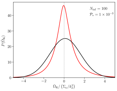
Figure 1: Probability distribution function for $\bar{\Omega}_{\mathrm{K}}=(aH/k_{\sigma})^{2}\Omega_{\mathrm{K}}$ (red curve) for unrealistically large values of $\mathcal{P}_{*}=10^{-3}$ (and $N_{\mathrm{inf}}=100$), compared to a Gaussian of same mean and variance (black curve). Notice that the most probable value of $\bar{\Omega}_{\mathrm{K}}$ is slightly negative whereas the mean value remains slightly positive.

The probability density function of $\Omega_{\mathrm{K}}$ can be determined by noticing that Eqs. 10 and 11 imply that $\Omega_{\mathrm{K}}$ can be seen as a non-linear functional over five stochastic Gaussian variables, ${\bf\it\Xi}\equiv(\xi,\Delta\xi,\vnabla\xi)$. As such, defining $\bar{\Omega}_{\mathrm{K}}\equiv(a^{2}H^{2}/k_{\sigma}^{2})\Omega_{\mathrm{K}}$ and marginalizing over the five-dimensional space associated with ${\bf\it\Xi}$, one has

$$P(\bar{\Omega}_{\mathrm{K}})=\int\dfrac{\differential[5]{\bf\it\Xi}}{\left(2\pi\right)^{5/2}}\,\delta\left(\bar{\Omega}_{\mathrm{K}}+\dfrac{K}{k_{\sigma}^{2}}e^{-2\xi}\right)\dfrac{e^{-\frac{1}{2}{\bf\it\Xi}^{\mathrm{T}}{\bf\it\Sigma}^{-1}{\bf\it\Xi}}}{\sqrt{\det{\bf\it\Sigma}}},$$ (43)

where the five-dimensional covariance matrix ${\bf\it\Sigma}$ is completely determined by the diagrammatic rules of Eq. 24. All but one integral appearing in Eq. 43 can be analytically reduced, and, after some algebra, one obtains

$$P(\bar{\Omega}_{\mathrm{K}}) =\dfrac{k_{\sigma}^{2}}{4\pi}\sqrt{\dfrac{27\sqrt{2}\Sigma_{\omega}}{\expectationvalue{\xi^{2}}\absolutevalue{\expectationvalue{K}}^{3}}}\int_{-\infty}^{+\infty}\differential x\,e^{-\frac{x^{2}}{2\expectationvalue{\xi^{2}}}+2x}$$ (44)

$$\times e^{-\frac{1}{2}\bar{\omega}^{2}(\bar{\Omega}_{\mathrm{K}},x)}H_{-\frac{3}{2}}\!\left[\dfrac{3\Sigma_{\omega}}{\sqrt{8}\absolutevalue{\expectationvalue{K}}}-\dfrac{\bar{\omega}(\bar{\Omega}_{\mathrm{K}},x)}{\sqrt{2}}\right],$$

where we have defined

$$\Sigma_{\omega}^{2} \equiv\expectationvalue{K_{1}^{2}}-4\dfrac{\expectationvalue{K}^{2}}{\expectationvalue{\xi^{2}}},$$ (45)

$$\bar{\omega}(\bar{\Omega}_{\mathrm{K}},x) \equiv e^{2x}\dfrac{\bar{\Omega}_{\mathrm{K}}}{(\Sigma_{\omega}/k_{\sigma}^{2})}+\dfrac{2\absolutevalue{\expectationvalue{K}}}{\expectationvalue{\xi^{2}}\Sigma_{\omega}}x.$$

In Eq. 44, $H_{\nu}\!\left(x\right)$ stands for the generalized Hermite polynomial of fractional order, defined from the parabolic cylinder functions Gradshteyn and Ryzhik (1980) as $H_{\nu}\!\left(x\right)\equiv 2^{\nu/2}e^{x^{2}/2}D_{\nu}(\sqrt{2}x)$. This distribution shows that, for $\expectationvalue{\xi^{2}}\simeq\mathcal{P}_{*}N_{\mathrm{inf}}\ll 1$, one can use the approximation

$$e^{-\frac{x^{2}}{2\expectationvalue{\xi^{2}}}+2x}\simeq\sqrt{2\pi\expectationvalue{\xi^{2}}}e^{2\expectationvalue{\xi^{2}}}\delta\left(x-2\expectationvalue{\xi^{2}}\right),$$ (46)

to simplify the integral over $x$ in Eq. 44. Remarking that, in this limit, the argument of the Hermite function is dominated by the first term, which is a constant scaling as $1/\sqrt{\mathcal{P}_{*}}$, $P(\bar{\Omega}_{\mathrm{K}})$ is, therefore, close to a Gaussian distribution over the quantity $\bar{\omega}(\bar{\Omega}_{\mathrm{K}},2\expectationvalue{\xi^{2}})$. In other words, for $\expectationvalue{\xi^{2}}\ll 1$, the distribution of $\bar{\Omega}_{\mathrm{K}}$ is almost Gaussian, with a width given by $\Sigma_{\omega}/k_{\sigma}^{2}\simeq\sqrt{\mathcal{P}_{*}}/3$ and a peak located at a very small negative value:

$$\left.\bar{\Omega}_{\mathrm{K}}\right|_{\max}\simeq\dfrac{4}{k_{\sigma}^{2}}\expectationvalue{K}e^{-4\expectationvalue{\xi^{2}}}\simeq-\dfrac{2}{3}\mathcal{P}_{*}.$$ (47)

For the curvature parameter today, one would get the most probable value at $\left.\Omega_{\mathrm{K}_{0}}\right|_{\max}\simeq-1.4\times 10^{-9}$, a barely closed universe were we to interpret this number within a FLRW metric with trivial topology. Let us notice the different sign than the mean value of Eq. 31; the distribution is indeed slightly skewed by the Hermite function. This can be seen in Fig. 1, where we have plotted $P(\bar{\Omega}_{\mathrm{K}})$ for an unrealistically large value of $\mathcal{P}_{*}=10^{-3}$. These distortions are also apparent in the odd moments of Eq. 42 which are, as already noted, all proportional to $\sqrt{\mathcal{P}_{*}}$.

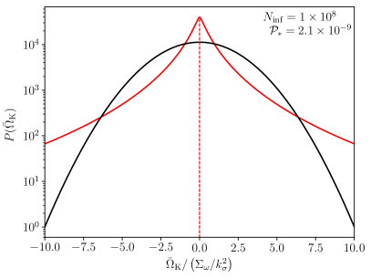
Figure 2: Probability distribution function for $\bar{\Omega}_{\mathrm{K}}=(aH/k_{\sigma})^{2}\Omega_{\mathrm{K}}$ (red curve) for the currently favored value of $\mathcal{P}_{*}=2.1\times 10^{-9}$ and for a large number of $e$-folds $N_{\mathrm{inf}}=10^{8}$. The variance $\expectationvalue{\xi^{2}}$ is no longer a small quantity and the distribution acquires heavy tails. Even though the width at half-maximum is $\order{\sqrt{\mathcal{P}_{*}}}$, substantial values of $|\bar{\Omega}_{\mathrm{K}}|$ are not rare anymore. For comparison, the black curve shows a Gaussian of same mean and variance.

When $\expectationvalue{\xi^{2}}\simeq\mathcal{P}_{*}N_{\mathrm{inf}}$ increases, Eq. 46 is no longer accurate, and all the terms of Eq. 44 are relevant. The distribution now acquires heavy tails, kicking in at increasingly smaller values of $\left|\bar{\Omega}_{\mathrm{K}}\right|$ and erasing the Gaussian profile in the neighborhood of $\left.\bar{\Omega}_{\mathrm{K}}\right|_{\max}$. In Fig. 2, we have plotted $P(\bar{\Omega}_{\mathrm{K}})$, in logarithmic scales, for $\mathcal{P}_{*}=2.1\times 10^{-9}$ and for a large number of $e$-folds $N_{\mathrm{inf}}=10^{8}$. These heavy tails imply that large values of $|\Omega_{\mathrm{K}_{0}}|$ are (much) more likely than what a Gaussian profile would imply. Their existence is also manifest in the moments of Eq. 42 through the exponential coefficients involving $\expectationvalue{\xi^{2}}$. Such an effect is reminiscent of the non-linear mapping of vacuum quantum fluctuations encountered in the context of stochastic inflation Pattison et al. (2017); Ezquiaga et al. (2020).

Finally, let us mention that numerical computations of $\expectationvalue{\Omega_{\mathrm{K}}}$ and $\expectationvalue{\Omega_{\mathrm{K}}^{2}}$ based on using the distribution of Eq. 44 do match the values we can get from Eqs. 30 and 36.

IV Discussion

If inflation lasts for a long period, then substantial values of $\Omega_{\mathrm{K}_{0}}$ might be produced. Indeed, letting $\sigma^{2}\simeq e^{-\expectationvalue{\xi^{2}}}$ to implement the condition stated below Eq. 15, Eq. 37 becomes $\expectationvalue{\Omega_{\mathrm{K}_{0}}^{2}}^{1/2}\simeq\sqrt{\mathcal{P}_{*}}e^{3\mathcal{P}_{*}N_{\mathrm{inf}}}/3$. For this value not to exceed the current observational bound $|\Omega_{\mathrm{K}_{0}}|<3\times 10^{-3}$, with $\mathcal{P}_{*}=2.1\times 10^{-9}$ this leads to $N_{\mathrm{inf}}<7\times 10^{8}$. On the one hand, this suggests that scenarios leading to phases of inflation lasting for more than a billion $e$-folds might be disfavored by current cosmological data. On the other hand, future cosmological surveys, such as the ones using the neutral hydrogen line at 21 cm, may possibly detect a non-vanishing curvature if inflation actually lasted slightly less than a billion $e$-folds Witzemann et al. (2018). Notice that the aforementioned bound becomes more stringent if one accounts for the slightly red observed spectral index.

Let us note, however, that when the above bound on $N_{\mathrm{inf}}$ is saturated, $\expectationvalue{\xi^{2}}\simeq 1.5$. A priori, our non-linear formulas do not require $\expectationvalue{\xi^{2}}$ to be small; hence, they can still be used in that case. In particular, although one can see that all the moments are becoming exponentially large with $\expectationvalue{\xi^{2}}$, Eq. 44 shows that $P(\bar{\Omega}_{\mathrm{K}})$ remains well defined. Nonetheless, the fact that the scale $k_{\sigma}$ must be set in a way that accommodates potentially large values of $\zeta$ suggests that our formalism may not be best suited in that case, and the upper bound we have obtained on $N_{\mathrm{inf}}$ must be taken with care. Moreover, for large $\expectationvalue{\xi^{2}}$, possible backreaction effects on super-Hubble scales could also induce deviations from Gaussianity.

If inflation lasts even longer, $\Omega_{\mathrm{K}}$ gets even larger, and our formalism needs to be extended in at least two ways. First, when $|\Omega_{\mathrm{K}}|$ becomes of the order unity, or more, the metric associated with Eq. 1 is not acceptable anymore. For instance, a large negative curvature density parameter would imply a compact manifold, and this demands another coordinate system than the one in Eq. 1. Second, when $|\Omega_{\mathrm{K}}|$ becomes sizable, it opens up a channel of backreaction of the curvature perturbation onto the background dynamics, which, in turn, alters the inflationary amplification of the curvature perturbations themselves Handley (2019); Letey et al. (2022). This mechanism might be tractable in an extended stochastic-inflation formalism Starobinsky (1986); Goncharov et al. (1987); Starobinsky and Yokoyama (1994); Vennin and Starobinsky (2015); Grain and Vennin (2021), which we plan to develop in a future work.

Finally, let us insist that our derivation of the statistics of $\Omega_{\mathrm{K}}$ is not rooted in any perturbative expansion of metric coefficients. The assumptions made are that $\zeta$ is of Gaussian statistics and conserved on super-Hubble scales. As such, our results would be modified if curvature perturbations are non-Gaussian at non-observably large scales. This is, strictly speaking, not excluded, although it would require very specific early-universe models for which curvature perturbations are Gaussian at observable scales today (in order to satisfy the tight constraints on non-Gaussianities Akrami et al. (2020a)) and non-Gaussian at larger scales. Another hypothesis that could be broken is that $\xi$ is conserved by adiabaticity. The presence of entropic modes today could invalidate this assumption, but, as for non-Gaussianities, their presence during inflation is also disfavored by current data.