Bifurcation and fission in the liquid drop model:
a phase-field approachthanks: This work is supported in part by the National Science Foundation DMS-2012562 and DMS-1937254.

Zirui Xu  and  Qiang Du (corresponding author) Department of Applied Physics and Applied Mathematics, Columbia University, New York, NY 10027, USA. Email: zx2250@columbia.edu.Department of Applied Physics and Applied Mathematics, and Data Science Institute, Columbia University, New York, NY 10027, USA. Email: qd2125@columbia.edu.

Abstract

The liquid drop model, originally used to model atomic nuclei, describes the competition between surface tension and Coulomb force. To help understand how a ball loses stability and becomes prone to fission, we calculate the minimum energy path of the fission process, and study the bifurcation branch conjectured by Bohr and Wheeler. We then present the two-dimensional analogue for comparison. Our study is conducted with the help of numerical simulations via a phase-field approach.

1 Introduction

The competition between attractive and repulsive interactions gives rise to a wide variety of pattern formation phenomena, ranging from polymer systems to ferroelectric/ferromagnetic systems to quantum systems to reaction-diffusion systems [47, 48]. It also accounts for the structure of nuclear matter in the crust of neutron stars [41]. One of the earliest theoretical studies in the literature is the liquid drop model of the atomic nucleus conceived by Gamow in 1928, which captures the competition between the attractive short-range nuclear force and the repulsive long-range Coulomb force [12]. Another relevant study is the Ohta–Kawasaki free energy introduced in 1986 to model the self-assembly of diblock copolymers [12, Equation (5)]. Because of their abilities to reproduce various fine mesoscopic structures found in block copolymers and many other systems, the Ohta–Kawasaki free energy and its variants have drawn wide mathematical interests (see, e.g., [70] and the references therein). In a mathematical study by Choksi and Peletier [13], the liquid drop model resurfaced as the leading-order term of the Ohta–Kawasaki free energy in the vanishing volume limit [12, Top-right of Page 1277]. Since then the liquid drop model started receiving much more attention from the mathematical community (see, e.g., [4, 25, 22] and many references therein), serving as an exemplary model of pattern formation driven by energetic competitions.

The liquid drop model was originally used to model the shape of the atomic nucleus. Although an atomic nucleus typically makes up more than 99.9% of the atomic mass, it occupies much less than 0.01% of the atomic volume. In fact, its diameter ranges from 2 to 12 fm (note that 1 fm equals $10^{-15}$ m), much smaller than the resolution of the best microscope [18, Page 16]. This means that in nuclear physics, the shape of the very object under study cannot be seen by any microscope. Nonetheless, the shape of a nucleus is a basic notion in theoretical models of nuclear structure and reactions [34]. A proper description of nuclear shapes is essential for explaining and theoretically studying nuclear activities such as nuclear fission [35]. In the liquid drop model, the atomic nucleus is treated as a drop of incompressible and uniformly charged fluid [12], therefore its energy is given by the surface energy plus the Coulomb potential energy. More precisely, for a nucleus occupying a domain $\Omega\subseteq\mathbb{R}^{3}$, up to some rescaling, the energy is given by (1). The volume $V$ of $\Omega$ is related to the mass number, i.e, the number of nucleons. Nucleons are bound together by the attractive nuclear force, so the nucleons on the surface of the nucleus lack neighbors and have higher potential energy, thus giving rise to the surface energy term. Despite its simplicity, the liquid drop model offers satisfactory explanations for the gross properties of nuclei such as the overall trend in the binding energy.

For a measurable set $\Omega\subseteq\mathbb{R}^{3}$, we consider the following energy functional [12, Equation (1)]

$$I(\Omega):=\text{Per}\,\Omega+\frac{1}{2}\int_{\Omega}\int_{\Omega}G(\vec{x},\vec{y})\differential{\vec{x}}\differential{\vec{y}},\quad G(\vec{x},\vec{y})=\frac{1}{4\pi|\vec{x}\!-\!\vec{y}|},$$ (1)

under the volume constraint $|\Omega|=V:=40\pi\raisebox{2.0pt}{$\chi$}$, where $\chi$ is the so-called fissility parameter, and Per$\,\Omega$ denotes the surface area of $\Omega$ (or the perimeter of $\Omega$ in the 2-D case). Note that in 2-D we define $G(\vec{x},\vec{y})=-\ln|\vec{x}\!-\!\vec{y}|/(2\pi)$ and $\raisebox{2.0pt}{$\chi$}=(V/\pi)^{3/2}\big{/}12$, where $V$ is the area of $\Omega$. In the physics literature [43, Page 2], the fissility parameter is denoted as $x$. We use the notation $\chi$ to avoid confusion with $\vec{x}$. We hereinafter focus on the 3-D case which has relevance to nuclear physics. Under the volume constraint, a ball minimizes the first term in (1) due to the isoperimetric inequality, but maximizes the second term due to Riesz rearrangement inequality [14, Page 755]. For $\raisebox{2.0pt}{$\chi$}\ll 1$, the first term is dominant, and the global minimizer $\Omega$ of $I=I(\Omega)$ is expected to be a ball; for $\raisebox{2.0pt}{$\chi$}\gg 1$, the second term is dominant, and $\Omega$ is expected to split into many fragments in order to prevent the second term from growing too large. In fact, as $\chi$ exceeds $\raisebox{2.0pt}{$\chi$}_{2}:=(\sqrt[3]{2}+\sqrt[3]{4})^{-1}\approx 0.351$, a single ball starts to have higher energy than two balls of equal radii infinitely far apart [14, Page 755].

According to [26, Page 4437 and Theorem 3.4] and [25] (see also [46, 38, 4, 44]), there exist $0<\raisebox{2.0pt}{$\chi$}_{2}^{-}\leqslant\raisebox{2.0pt}{$\chi$}_{2}^{+}\leqslant 4/5$ such that:

  1. 1

    for $\raisebox{2.0pt}{$\chi$}<\raisebox{2.0pt}{$\chi$}_{2}^{-}$, a ball is the unique global minimizer (up to translation);

  2. 2

    for $\raisebox{2.0pt}{$\chi$}=\raisebox{2.0pt}{$\chi$}_{2}^{-}$, a ball is a global minimizer;

  3. 3

    for $\raisebox{2.0pt}{$\chi$}>\raisebox{2.0pt}{$\chi$}_{2}^{-}$, a ball is not a global minimizer;

  4. 4

    for $\raisebox{2.0pt}{$\chi$}\in(0,\raisebox{2.0pt}{$\chi$}_{2}^{+}]\backslash O$ with some open set $O\subseteq(\raisebox{2.0pt}{$\chi$}_{2}^{-},\raisebox{2.0pt}{$\chi$}_{2}^{+})$, there is a global minimizer;

  5. 5

    for $\raisebox{2.0pt}{$\chi$}\in(\raisebox{2.0pt}{$\chi$}_{2}^{+},\infty)\cup O$, there is no global minimizer.

Obviously $\raisebox{2.0pt}{$\chi$}_{2}^{-}\leqslant\raisebox{2.0pt}{$\chi$}_{2}$. It is widely believed but not proved that $\raisebox{2.0pt}{$\chi$}_{2}^{-}=\raisebox{2.0pt}{$\chi$}_{2}^{+}=\raisebox{2.0pt}{$\chi$}_{2}$ [14, Page 755]. For $\chi$ not very small, the global minimizer is not rigorously known. However, several qualitative results are known. According to [12, Bottom-right of Page 1280] and [4, Theorem 2.7], any local minimizer has $C^{\infty}$ reduced boundaries, and is essentially bounded with a finite number of connected components; moreover, any global minimizer is connected. According to [39, Theorem 1], any $C^{2}$-regular critical set has analytic boundaries. Although there is no global minimizer for $\raisebox{2.0pt}{$\chi$}\in(\raisebox{2.0pt}{$\chi$}_{2}^{+},\infty)\cup O$, a generalized global minimizer always exists, consisting of a finite collection of connected components which are infinitely far apart (with each component bounded, connected and $C^{\infty}$-regular after a zero Lebesgue measure modification) [41, Theorem 4.5].

For any $\raisebox{2.0pt}{$\chi$}>0$, a ball is always a stationary point of $I$ (i.e., a regular critical set in the sense of [4, Definition 2.5]). Note that a stationary point is not necessarily stable. In fact, a ball is strictly stable for $\raisebox{2.0pt}{$\chi$}<\raisebox{2.0pt}{$\chi$}_{*}:=1$ and unstable for $\raisebox{2.0pt}{$\chi$}>\raisebox{2.0pt}{$\chi$}_{*}$ [4, Theorem 2.9]. By “strictly stable” we mean that for $\raisebox{2.0pt}{$\chi$}<\raisebox{2.0pt}{$\chi$}_{*}$, a ball is an isolated local minimizer in the sense of [4, Definition 2.4]. Thus, for $\raisebox{2.0pt}{$\chi$}\in(\raisebox{2.0pt}{$\chi$}_{2},\raisebox{2.0pt}{$\chi$}_{*})$, a ball remains an isolated local minimizer although it is no longer a global minimizer. Notice that the stability is often defined in the $L^{1}$-topology [42, Equations (2.1) and (2.8)] or $L^{2}$-topology [55, Bottom of Page 911]. Furthermore, strict stability may be defined modulo translation (see [1, Definition 2.4] and [4, Definition 2.4]). It is known that strict stability can be deduced from strict positivity of the second variation (modulo translation) of a $C^{1}$-regular critical set [4, Theorem 2.8]. It should be analogous to define strict stability modulo both translation and rotation, although we have not seen such a definition in the literature.
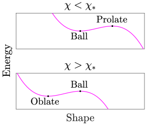
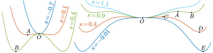
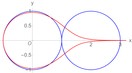
For $\chi$ slightly larger than $\raisebox{2.0pt}{$\chi$}_{*}$, we are interested to see what will happen to a ball after it loses its stability and ceases to be a local minimizer. For $\raisebox{2.0pt}{$\chi$}\approx\raisebox{2.0pt}{$\chi$}_{*}$, a smooth family of stationary points has been constructed in [24]. Every member of this family is axisymmetric and resembles a prolate 111 Throughout this paper, we regard “oblate” and “prolate” as nouns instead of adjectives, and refer to the interiors of oblate and prolate spheroids, respectively. (for $\raisebox{2.0pt}{$\chi$}<\raisebox{2.0pt}{$\chi$}_{*}$), a ball (for $\raisebox{2.0pt}{$\chi$}=\raisebox{2.0pt}{$\chi$}_{*}$), or an oblate (for $\raisebox{2.0pt}{$\chi$}>\raisebox{2.0pt}{$\chi$}_{*}$), as shown on the left of Figure 1. This family is illustrated as the tilted line on the right of Figure 1 (where the vertical axis qualitatively represents the shape, e.g., the height to width ratio). According to [24, Page 071506-2], this family exchanges stability with the ball at $\raisebox{2.0pt}{$\chi$}=\raisebox{2.0pt}{$\chi$}_{*}$, where a transcritical bifurcation happens. More specifically, for $\raisebox{2.0pt}{$\chi$}<\raisebox{2.0pt}{$\chi$}_{*}$, the prolate-like stationary point is unstable and has higher energy than the ball; for $\raisebox{2.0pt}{$\chi$}>\raisebox{2.0pt}{$\chi$}_{*}$, the oblate-like stationary point is “stable” and has lower energy than the ball. Therefore it seems reasonable to speculate that as $\chi$ slightly exceeds $\raisebox{2.0pt}{$\chi$}_{*}$, the ball will deform slightly into a stable oblate-like equilibrium.

prolateRefer to captionRefer to captionprolate\overset{\includegraphics[width=47.328pt]{images/Spheroid/prolate.png}}{\text{prolate}} ballRefer to captionRefer to captionball\overset{\raisebox{3.0pt}{\includegraphics[width=52.2pt]{images/Spheroid/sphere.png}}}{\text{ball}} oblateRefer to captionRefer to captionoblate\overset{\raisebox{4.5pt}{\includegraphics[width=57.42pt]{images/Spheroid/oblate.png}}}{\text{oblate}}        prolate-likeoblate-like$\raisebox{2.0pt}{$\chi$}\!>\!\raisebox{2.0pt}{$\chi$}_{*}$ball$\raisebox{2.0pt}{$\chi$}\!<\!\raisebox{2.0pt}{$\chi$}_{*}$ball

Figure 1: Left: three types of spheroids. Right: transcritical bifurcation diagram, where the solid and dashed lines indicate stable and unstable branches, respectively.

Upon closer scrutiny, however, we note that those oblate-like stationary points have only been proved to be stable against certain axisymmetric perturbations [24, Corollary 5]. In fact, as shown in Section 4.1, our numerical simulations indicate that they are unstable against non-axisymmetric perturbations and will eventually split into two disconnected components. In other words, symmetry breaking occurs. Usually in a transcritical bifurcation, the unstable branch exchanges stability with the stable branch and becomes stable when the parameter exceeds the critical value [62, Pages 51 and 244]. But as mentioned above, we believe that both the prolate-like and oblate-like branches are unstable, and we will explain this counter-intuitive phenomenon in Section 4.5.
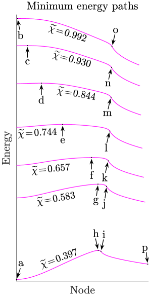
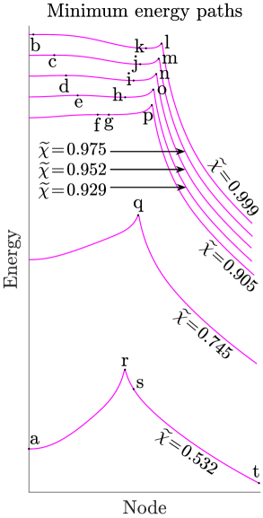
For $\raisebox{2.0pt}{$\chi$}<\raisebox{2.0pt}{$\chi$}_{*}$, we are interested in the minimum energy path of the fission process. To the best of our knowledge, in the literature people have not obtained complete fission paths without severe restrictions on the admissible shapes of the nucleus. Using the string method [68], we are able to obtain complete fission paths (see Section 4.2). With the help of the shrinking dimer method [71], we are able to obtain the saddle point along the fission path. Such a saddle point, also called a transition state 222 A transition state is a point of locally highest energy along the minimum energy path., is of particular interest, because it is related to the activation energy required for the nuclear fission to take place. In 1939, Bohr and Wheeler [3] studied those saddle points and obtained the leading-order behaviors for $\raisebox{2.0pt}{$\chi$}\approx\raisebox{2.0pt}{$\chi$}_{*}$ using a Legendre polynomial expansion. Such asymptotic results were justified rigorously by Frank [24], who proved the existence (and uniqueness) of those saddle points for $\raisebox{2.0pt}{$\chi$}\approx\raisebox{2.0pt}{$\chi$}_{*}$ (see Figure 1). In addition, Bohr and Wheeler conjectured that this bifurcation branch can be extended from $\raisebox{2.0pt}{$\chi$}\approx\raisebox{2.0pt}{$\chi$}_{*}$ to arbitrarily small $\chi$, with the saddle point changing from spheroid-like shapes to dumbbell-like shapes and then converging to two touching balls of equal sizes [3, Figure 2]. This conjecture remains open, since the proof given by Frank is only valid in a small neighborhood of $\raisebox{2.0pt}{$\chi$}=\raisebox{2.0pt}{$\chi$}_{*}$ [24, Page 071506-2]. In the literature, numerical calculation of the Bohr–Wheeler branch is scarce [12, Top right of Page 1280]. Using a phase-field approach, we are able to numerically compute the entire Bohr–Wheeler branch, as shown in Figure 2, thus providing numerical supports for their conjecture. Note that our computation covers the entire range of $\chi$, i.e., $\raisebox{2.0pt}{$\chi$}\in(0,\raisebox{2.0pt}{$\chi$}_{5})$, with $\raisebox{2.0pt}{$\chi$}_{5}\approx 1.8$ corresponding to a discocyte-like stationary point whose two faces touch each other. In the literature we have not seen any numerical calculation of the portion $\raisebox{2.0pt}{$\chi$}\in(\raisebox{2.0pt}{$\chi$}_{*},\raisebox{2.0pt}{$\chi$}_{5})$.

0.124Refer to caption\overset{\includegraphics[width=70.0pt,bb=0 0 284 291]{images/BifurcationBranch/p1.0.png}}{\text{0.124}\quad} 0.248Refer to caption\overset{\includegraphics[width=70.0pt,bb=0 0 284 291]{images/BifurcationBranch/p2.0.png}}{\text{0.248}\quad} 0.397Refer to caption\overset{\includegraphics[width=70.0pt,bb=0 0 284 291]{images/BifurcationBranch/p3.2.png}}{\text{0.397}\quad} 0.583Refer to caption\overset{\includegraphics[width=70.0pt,bb=0 0 284 291]{images/BifurcationBranch/p4.7.png}}{\text{0.583}\quad} 0.657Refer to caption\overset{\includegraphics[width=70.0pt,bb=0 0 284 291]{images/BifurcationBranch/p5.3.png}}{\text{0.657}\quad} 0.744Refer to caption\overset{\includegraphics[width=70.0pt,bb=0 0 284 291]{images/BifurcationBranch/p6.0.png}}{\text{0.744}\quad}
         0.844Refer to caption\overset{\includegraphics[width=70.0pt,bb=0 0 284 291]{images/BifurcationBranch/p6.8.png}}{\text{0.844}\quad} 0.930Refer to caption\overset{\includegraphics[width=70.0pt,bb=0 0 284 291]{images/BifurcationBranch/p7.5.png}}{\text{0.930}\quad} 0.992Refer to caption\overset{\includegraphics[width=70.0pt,bb=0 0 284 291]{images/BifurcationBranch/p8.0.png}}{\text{0.992}\quad} 1.054Refer to caption\overset{\includegraphics[width=70.0pt,bb=0 0 284 291]{images/BifurcationBranch/o8.5.png}}{\text{1.054}\quad} 1.116Refer to caption\overset{\includegraphics[width=70.0pt,bb=0 0 284 291]{images/BifurcationBranch/o9.png}}{\text{1.116}\quad} 1.178Refer to caption\overset{\includegraphics[width=70.0pt,bb=0 0 284 291]{images/BifurcationBranch/o9.5.png}}{\text{1.178}\quad}
1.240Refer to caption\overset{\includegraphics[width=70.0pt,bb=0 0 284 291]{images/BifurcationBranch/o10.png}}{\text{1.240}\quad} 1.365Refer to caption\overset{\includegraphics[width=70.0pt,bb=0 0 284 291]{images/BifurcationBranch/o11.png}}{\text{1.365}\quad} 1.489Refer to caption\overset{\includegraphics[width=70.0pt,bb=0 0 284 291]{images/BifurcationBranch/o12.png}}{\text{1.489}\quad} 1.613Refer to caption\overset{\includegraphics[width=70.0pt,bb=0 0 284 291]{images/BifurcationBranch/o13.png}}{\text{1.613}\quad} 1.737Refer to caption\overset{\includegraphics[width=70.0pt,bb=0 0 284 291]{images/BifurcationBranch/o14.png}}{\text{1.737}\quad} 1.799Refer to caption\overset{\includegraphics[width=70.0pt,bb=0 0 284 291]{images/BifurcationBranch/o14.5.png}}{\text{1.799}\quad}

Figure 2: Computed Bohr–Wheeler bifurcation branch. Below each shape is $\widetilde{\chi}$.

In Figure 2, the simulation box is a unit cube. The shapes are rescaled and their volumes are 0.09. They are axisymmetric, and the axes of revolution for the first nine shapes are chosen to be a body diagonal of the cube, while those for the last nine are chosen to be a vertical line passing through the center of the cube. As discussed in Section 3.1, $\widetilde{\chi}$ is the phase-field approximation of $\chi$. Following the terminology in [52], if an axisymmetric object lacks mirror symmetry perpendicular to the axis of revolution, then we call it mass-asymmetric (e.g., a bowling pin or an European pear that has a heavier bottom and a lighter top). There is a critical value $\raisebox{2.0pt}{$\chi$}_{3}\approx 0.395\pm 0.001$ (the so-called Businaro–Gallone point), such that for $\raisebox{2.0pt}{$\chi$}<\raisebox{2.0pt}{$\chi$}_{3}$, the saddle point becomes unstable to mass-asymmetric perturbations, that is, the two ends of the dumbbell-like shape tend to develop size inequality, until one of them vanishes and the dumbbell becomes a ball (see Section 4.3). In other words, as $\chi$ drops below $\raisebox{2.0pt}{$\chi$}_{3}$, the saddle point gains one more unstable direction and its index increases from 1 to 2.

To understand the fate of the Bohr–Wheeler branch after it disappears when $\chi$ exceeds $\raisebox{2.0pt}{$\chi$}_{5}$, we carry out numerical simulations for $\raisebox{2.0pt}{$\chi$}>\raisebox{2.0pt}{$\chi$}_{5}$. We observe that the discocyte-like shape on the Bohr–Wheeler branch changes hysteretically to a torus-like shape on a separate branch (see Appendix I). As $\chi$ increases, such a torus-like equilibrium expands and becomes thinner. For $\chi$ large enough, equilibria on this branch have been found by Ren and Wei [59]. As $\chi$ decreases, such a torus-like shape constricts and thickens, and disappears for $\raisebox{2.0pt}{$\chi$}<\raisebox{2.0pt}{$\chi$}_{4}\approx 0.972$, through what we believe is a saddle-node bifurcation.

A summary of the above-mentioned qualitative changes is illustrated in Figure 3. For $\raisebox{2.0pt}{$\chi$}=0$, we recover the classical isoperimetric problem upon rescaling [38, Equation (2.1)], and any local minimizer must be a ball [19]. In a tiny neighborhood of $\raisebox{2.0pt}{$\chi$}=0$, Julin proved a similar result: for any $M>0$, there is a $\varepsilon>0$ such that for any $\raisebox{2.0pt}{$\chi$}\in(0,\varepsilon)$, if a smooth local minimizer of (1) satisfies $\text{Per}\,\Omega\leqslant M|\Omega|^{2/3}$, then it must be a ball [24, Top of Page 071506-2]. As $\chi$ exceeds $\raisebox{2.0pt}{$\chi$}_{1}:=1/5$ and $\raisebox{2.0pt}{$\chi$}_{2}$, the shape consisting of two balls of equal radii infinitely far apart becomes a generalized local minimizer (see Appendix A) and a generalized global minimizer (conjectured but unproved), respectively. Once $\chi$ exceeds $\raisebox{2.0pt}{$\chi$}_{3}$, the Bohr–Wheeler branch changes the degree of instability from 2 to 1. In other words, $\raisebox{2.0pt}{$\chi$}_{3}$ is where the dumbbell-like saddle point changes stability against mass-asymmetric perturbations, whereas $\raisebox{2.0pt}{$\chi$}_{1}$ is where the shape consisting of two balls of equal radii infinitely far apart changes stability against mass-asymmetric perturbations. When $\chi$ exceeds $\raisebox{2.0pt}{$\chi$}_{4}$, the torus-like branch comes to existence. When $\chi$ exceeds $\raisebox{2.0pt}{$\chi$}_{*}$, the ball loses its local minimality and becomes unstable. When $\chi$ exceeds $\raisebox{2.0pt}{$\chi$}_{5}$, the Bohr–Wheeler branch ceases to exist.

00One ball is the onlylocal minimizer$\raisebox{2.0pt}{$\chi$}_{1}$Two-ball becomesa local minimizer$\raisebox{2.0pt}{$\chi$}_{2}$Two-ball becomesa global minimizer$\raisebox{2.0pt}{$\chi$}_{3}$Businaro–Gallonepoint$\raisebox{2.0pt}{$\chi$}_{4}$Torus-likebranch starts$\raisebox{2.0pt}{$\chi$}_{*}$One ball loseslocal minimality$\raisebox{2.0pt}{$\chi$}_{5}$Bohr–Wheelerbranch ends$\chi$
Figure 3: Several qualitative changes as $\chi$ increases.

So far we have only considered the 3-D case. The 2-D case is also interesting, since it corresponds to the cylindrical phase in the diblock copolymer systems [56, Page 880]. In 2-D, when a disk loses stability at $\raisebox{2.0pt}{$\chi$}=\raisebox{2.0pt}{$\chi$}_{*}$, we believe that it corresponds to a subcritical pitchfork bifurcation (unlike the transcritical bifurcation in 3-D). For $\chi$ slightly smaller than $\raisebox{2.0pt}{$\chi$}_{*}$, there is an intermediate “local minimizer” resembling a smooth connected non-convex Cassini oval, a shape that we refer to as an eye mask. The transition state from the eye mask to two disks resembles a lemniscate (see Section 4.4).

The rest of this paper is organized as follows. In Section 2 we compare the present work to related studies in the literature. In Section 3 we present our phase-field reformulation and numerical methods. In Section 4 we present our numerical results in 3-D and 2-D. In Section 5 we study the periodic isoperimetric problem involving only the perimeter term. In Section 6 we present asymptotic analysis of two touching balls (or disks) as $\raisebox{2.0pt}{$\chi$}\rightarrow 0$. In Section 7 we conclude with remarks about future directions.

2 Comparison with existing literature

In the literature, shape parametrizations are often empirically chosen and widely used in the study of the fission process. The nucleus is then restricted to a certain class of shapes, and the variational problem is reduced to an optimization problem in a finite dimension, e.g., 18 dimensions [17, Page 408]. With such a reduction, Cohen and Swiatecki [17, Figure 1a] obtained the portion $0.3\leqslant\raisebox{2.0pt}{$\chi$}\leqslant 1$ of the Bohr–Wheeler branch. However, it is questionable whether the chosen class of shapes can accurately approximate the true solution, especially for $\raisebox{2.0pt}{$\chi$}<0.28$ [17, Page 409].

In 2009, Ivanyuk and Pomorski [33, 35] managed to numerically solve the variational problem without relying on shape parameterizations. They assume the nucleus to be axisymmetric with a sharp interface, so that its shape can be described by the meridian of the surface of revolution. They then use iterations to solve the Euler–Lagrange equation subject to the volume constraint. In order to study fission, they introduce another constraint that fixes the elongation. The elongation is a functional which characterizes how elongated a shape is. For a sequence of different values of elongation, they obtain a sequence of shapes, which they think can depict the fission process (because during fission, the nucleus should become more and more elongated, intuitively). Their results therefore depend on the definition of elongation [35, Figure 3], although the dependence may be weak for good choices of definitions. However, the dependence becomes more noticeable when the elongation approaches its maximum, with the nucleus now resembling a dumbbell. Beyond this maximum elongation, no solution is obtained, rendering it difficult to study the later stages of fission (i.e., the rupture of the neck of the dumbbell and the separation of the nucleus into two fragments). As a workaround, Ivanyuk [34, Figure 6-(b)] carries out a similar calculation for two separate fragments and then pieces together the entire fission process. However, the resulting fission curve is non-smooth and possibly inaccurate. In other words, near the scission point, their method cannot handle topological changes effectively, due to its sharp interface description of the nuclear shape. Note that the scission point is where the nucleus is going through topological changes and about to be split into two fragments, a terminology from [17, Page 427] and [52]. Despite its importance, the scission point is not well understood [34]. Furthermore, it seems difficult to adapt Ivanyuk’s method to the case where the axisymmetric assumption is dropped.

In contrast, axisymmetry is not assumed in our phase-field simulations. With the nuclear shape described by a thin layer of diffuse interface, topological changes can be easily simulated. A similar attempt to numerically study the liquid drop model using the phase-field approach has already been made in [28, Section 5] for the 2-D case. Inevitably, we introduce an approximation error by changing a sharp interface problem into a diffuse interface problem, but our results suggest that the error is very small. Moreover, the sharp interface model itself is also an approximate description of the actual physics. For example, nuclear densities are said to have exponential tails rather than a sharp interface [43, Page 6] (see also [33, Section 6]). Our method can conveniently take into account the short (but nonzero) range of the nuclear force, by adjusting the diffuseness of the interface if necessary. We can simulate the entire fission process by calculating the minimum energy path, without the need to introduce an artificial definition of elongation. Our phase-field approach will have even more advantages when the shape is non-axisymmetric, e.g., if we also consider the angular momentum of the nucleus.

Businaro and Gallone in 1955, as well as Cohen and Swiatecki in 1962, stated that for $\raisebox{2.0pt}{$\chi$}>\raisebox{2.0pt}{$\chi$}_{*}$, the oblate-like stationary points on the Bohr–Wheeler branch are unstable against non-axisymmetric perturbations [50, Paragraph 2 in Page 211], but they did not provide evidence [66, Paragraph 1 in Page 69]. The present study provides convincing numerical evidence for this claim. It remains an open question to analytically prove that the oblate-like stationary points constructed by Frank [24] are indeed unstable against non-axisymmetric perturbations. As a side note, a similar symmetry breaking phenomenon occurs in a slightly different problem [50, Bottom of Page 225, Top of Page 218], where the liquid drop is assumed to be conductive and thus the charge is distributed only on the surface (although such a problem was later found to be ill-posed and thus regularization is needed [49]).

Nix [52, Bottom of Page 265] suspected that for $\raisebox{2.0pt}{$\chi$}\geqslant 0.78$, the minimum energy path of fission may involve three fragments, which was not allowed by the parametrization that was used (with only six degrees of freedom). Since our phase-field method does not make use of axisymmetric assumptions or any shape parametrizations, our numerical results confirm that the fission paths are indeed axisymmetric, and that there is no such three-fragments fission.

In the literature, it has been noticed that there is a rapid (but continuous) change in the shape of the saddle point on the Bohr–Wheeler branch around $\raisebox{2.0pt}{$\chi$}\approx 0.67$ [17, Abstract], and our results in Figure 2 seem to support this observation.

The Businaro–Gallone point is related to mass-asymmetric fission of light and medium nuclei. For $\raisebox{2.0pt}{$\chi$}>\raisebox{2.0pt}{$\chi$}_{3}$, the fission can proceed in a mass-symmetric manner, from a ball to a dumbbell and eventually to two separate balls. In other words, every point along this transition path is mass-symmetric, and the transition state is an index-1 saddle point whose energy defines a threshold energy (a notion used in [16, Page 144], equivalent to activation energy in transition state theory). For $\raisebox{2.0pt}{$\chi$}<\raisebox{2.0pt}{$\chi$}_{3}$, the saddle point is of index 2, so its energy does not define a threshold energy, and the process tends to pick a mass-asymmetric path. In extremely mass-asymmetric cases, where a very light fragment (consisting of only a few nucleons) is emitted from the parent nucleus, the process is called spallation [16, Page 144]. Below the Businaro–Gallone point, it is thought that there is no longer a distinction between fission and spallation [16, Paragraph 1 of Page 145], because the mass-symmetric fission path is not energetically preferable to mass-asymmetric paths. Our numerical simulations confirm the above qualitative statements (see Sections 4.2 and 4.3 as well as Appendix F). Businaro and Gallone [7] estimated $\raisebox{2.0pt}{$\chi$}_{3}$ to be 0.47. Later on Cohen and Swiatecki [17] determined $\raisebox{2.0pt}{$\chi$}_{3}$ to be approximately 0.394, Nix [52] and Thomas et al. [65] determined $\raisebox{2.0pt}{$\chi$}_{3}$ to be 0.396, and then Ivanyuk [36, Page 519] determined $\raisebox{2.0pt}{$\chi$}_{3}$ to be approximately 0.4. Our estimation $\raisebox{2.0pt}{$\chi$}_{3}\approx 0.395\pm 0.001$ is consistent with those existing results. In the physics literature, it is unknown if there is any instability against mass-asymmetric perturbations during the descent from the saddle point to the scission point [52, Middle of Page 242]. Nix suggested that there is likely no such instability [52, Bottom of Page 265]. Our results in Section 4.2 are consistent with Nix’s speculation.

As shown at the top-left of Figure 2, our results demonstrate that when $\chi$ is small, the saddle point on the Bohr–Wheeler branch resembles two equally large balls connected by a thin and short neck. We believe that it will converge to two equally large balls touching at a single point as $\raisebox{2.0pt}{$\chi$}\rightarrow 0$, as conjectured by Bohr and Wheeler [3, Figure 2-(a)]. We perform asymptotic analysis in Section 6 and calculate the asymptotic neck circumference as $\raisebox{2.0pt}{$\chi$}\rightarrow 0$.

3 Phase-field models and numerical methods

3.1 Phase-field approach

Phase-field methods are useful tools to quantitatively simulate interfaces and geometric motions such as those related to the microstructures found in materials or biological specimens, see [21] for a recent review. The basic idea is to use a narrow but diffuse interface in place of the sharp interface. The diffuse interface is described by a phase-field variable $\eta$ (also called an order parameter), which takes different values in different phases and has a rapid but smooth transition across interfaces from one phase to another, with a diffuseness parameter controlling the thickness of the interfacial layer. In phase-field models, there is no need to explicitly track the interfaces, since the governing equations are in a unified form throughout the domain of simulation. We reformulate the liquid drop energy (1) into a diffuse interface version. For a fixed diffuseness parameter which is small enough, we study the diffuse interface problem numerically and then infer similar properties about the sharp interface problem. Note that our diffuse interface formulation is very similar to the Ohta–Kawasaki free energy [15, Equation (6.37)].

We consider the following phase-field reformulation of (1)

$\displaystyle\tilde{I}(\eta):=$ $\displaystyle\sqrt{\frac{6}{c}}\int_{D}\!W\big{(}\eta(\vec{x})\big{)}\differential{\vec{x}}+\sqrt{\frac{3c}{2}}\!\int_{D}\big{|}\nabla\eta(\vec{x})\big{|}^{2}\differential{\vec{x}}+\frac{\tilde{\gamma}}{2}\!\int_{D}\int_{D}f\big{(}\eta(\vec{x})\big{)}G(\vec{x},\vec{y})f\big{(}\eta(\vec{y})\big{)}\differential{\vec{x}}\differential{\vec{y}}$ (2)
$\displaystyle+\frac{K}{2}\Big{(}\int_{D}f\big{(}\eta(\vec{x})\big{)}\differential{\vec{x}}-\omega|D|\Big{)}^{2},$

where $D\subseteq\mathbb{R}^{n}$ is the simulation box ($n\in\{2,3\}$, since the 1-D case has already been solved in [55]), $W(z):=3(z\!-\!z^{2})^{2}$, the diffuseness parameter $0<c\ll 1$ controls the interfacial thickness, the nonlocal coefficient $\tilde{\gamma}>0$ controls the strength of Coulomb interactions, $G$ is the Green’s function of the negative Laplacian $-\Delta$ on $D$ with suitable boundary conditions, $f(z):=3z^{2}-2z^{3}$, and $K\gg 1$ is the penalty coefficient for the volume constraint with $\omega$ being the volume fraction. As we will explain below (4), in order to make clear the physical meaning of the coefficient $\tilde{\gamma}$ in terms of the fissility parameter, we use the following reparametrization of $\tilde{\gamma}$,

$$\tilde{\gamma}=\frac{40\pi\raisebox{2.0pt}{$\widetilde{\chi}$}}{\omega|D|}\;\text{in 3-D\quad and}\quad\tilde{\gamma}=12\raisebox{2.0pt}{$\widetilde{\chi}$}\Big{(}\frac{\pi}{\omega|D|}\Big{)}^{3/2}\;\text{in 2-D}.$$ (3)

The double well potential $W$ has two minimum points at $z=0$ and $z=1$. In order for the first term of $\tilde{I}(\eta)$ to be minimized, $\eta$ should be equal to 0 or 1 almost everywhere. However, the second term of $\tilde{I}(\eta)$ penalizes rapid spatial variations in $\eta$. Since the coefficient $c$ is small, we expect a thin and smooth transition layer to separate the domains where $\eta\approx 0$ and $\eta\approx 1$, respectively.

The nonlinear function $f$ is a technique introduced in [67] to overcome some numerical difficulties. Since it satisfies $f(0)=0$ and $f(1)=1$, and we expect $\eta\approx 0$ or $\eta\approx 1$ at most places in $D$, the function $f$ has roughly the same effect on $\tilde{I}(\eta)$ as the identity function. In addition, since we have $f^{\prime}(0)=f^{\prime}(1)=0$, the solution $\eta$ can exhibit the desired two-phases profile, which would have required a much smaller $c$ and thus a much finer grid if we used the identity function instead of $f$. See [67] and [69, Section 4.1] for more details.

For clarity let us for a moment replace $f$ by the identity function, i.e., $f(z):=z$. In this way we can see that the third term of $\tilde{I}$ resembles the Coulomb potential energy term of $I$ in (1), and that the fourth term of $\tilde{I}$ is to penalize the violation of the volume constraint $\int_{D}\eta=\omega|D|$.

3.2 Sharp interface limit

As $K\rightarrow\infty$ and $c\rightarrow 0$, we expect that the minimizer $\eta$ converges to some indicator function $\bm{1}_{\Omega}$, and that the diffuse interface energy (2) $\Gamma$-converges to the sharp interface energy (1) up to some rescaling,

$$\tilde{I}(\eta)\overset{\Gamma}{\longrightarrow}\,\text{Per}\,\Omega+\frac{\tilde{\gamma}}{2}\big{\langle}\bm{1}_{\Omega},(-\Delta)^{-1}\bm{1}_{\Omega}\big{\rangle},\quad\text{subject to}\;|\Omega|=\omega|D|,$$

where $\langle\,\cdot\,,\,\cdot\,\rangle$ represents the $L^{2}$ inner product, and $(-\Delta)^{-1}$ is equipped with the same boundary conditions as (2). In fact, a related $\Gamma$-convergence result is proved in [55, Section 2] under Neumann boundary conditions.

In the variational problem (1), the nonlocal coefficient is fixed, and the only adjustable parameter is the volume of $\Omega$. Note that according to the scaling property [38, Equation (2.1)], adjusting the volume and adjusting the nonlocal coefficient are interchangeable, so we can fix the volume and adjust the nonlocal coefficient. More specifically, minimization of (1) is equivalent (upon rescaling) to minimizing

$$\text{Per}\,\Omega+\frac{\gamma}{2}\big{\langle}\bm{1}_{\Omega},(-\Delta)^{-1}\bm{1}_{\Omega}\big{\rangle},\quad\text{subject to}\;|\Omega|=\omega|D|,$$ (4)

where $\gamma=40\pi\raisebox{2.0pt}{$\chi$}/(\omega|D|)$ in 3-D, $\gamma=12\raisebox{2.0pt}{$\chi$}(\omega|D|/\pi)^{-3/2}$ in 2-D, and $(-\Delta)^{-1}$ is equipped with no boundary conditions since (1) is posed on the whole space.

In order to make it convenient to compare our results with the existing results in the physics literature, we define a new parameter $\widetilde{\chi}$ in (3) so that $\gamma/\raisebox{2.0pt}{$\chi$}=\tilde{\gamma}/\raisebox{2.0pt}{$\widetilde{\chi}$}$. In other words, $\widetilde{\chi}$ is the counterpart of $\chi$ in the diffuse interface setting. As mentioned before, in the sharp interface problem, a ball loses stability when $\raisebox{2.0pt}{$\chi$}=\raisebox{2.0pt}{$\chi$}_{*}$, where $\raisebox{2.0pt}{$\chi$}_{*}$ equals 1. However, we do not expect its counterpart $\raisebox{2.0pt}{$\widetilde{\chi}$}_{*}$ in the diffuse interface setting to be exactly 1, due to the error introduced by the diffuse interfaces. Nevertheless, we do expect $\raisebox{2.0pt}{$\widetilde{\chi}$}_{*}$ to converge to 1 as $K\rightarrow\infty$ and $c\rightarrow 0$.

3.3 Energy minimization

In order to find the local minimizers of $\tilde{I}$, we use the following $L^{2}$ gradient flow, which is also called the penalized Allen–Cahn–Ohta–Kawasaki (pACOK) dynamics [69, Equation (1.13)]:

$$\frac{\partial\eta}{\partial t}=-\frac{\delta\tilde{I}(\eta)}{\delta\eta}=-\sqrt{6/c}\,W^{\prime}(\eta)+\sqrt{6c}\,\Delta\hskip 0.5pt\eta+\tilde{\gamma}f^{\prime}(\eta)\,\Delta^{-1}f(\eta)-Kf^{\prime}(\eta)\big{\langle}f(\eta)\!-\!\omega,\,1\big{\rangle},$$ (5)

with a given initial value of $\eta$ at $t=0$, where $t$ is the time variable, and $\Delta^{-1}$ is equipped with the same boundary conditions as (2). It is easy to see $W^{\prime}(z)=12z^{3}\!-\!18z^{2}\!+\!6z$ and $f^{\prime}(z)=6z\!-\!6z^{2}$. Therefore any stationary point of $\tilde{I}$ should satisfy

$$\sqrt{6/c}\,W^{\prime}(\eta)-\sqrt{6c}\,\Delta\hskip 0.5pt\eta-\tilde{\gamma}f^{\prime}(\eta)\,\Delta^{-1}f(\eta)=-Kf^{\prime}(\eta)\big{\langle}f(\eta)\!-\!\omega,\,1\big{\rangle}.$$ (6)

Analogously, any stationary point of the sharp interface energy (4) satisfies the following equation [57, Equation (1.1)] (see also [12, Equation (6)])

$$(n\!-\!1)H+\gamma\phi=\lambda\;\text{on}\;\partial\Omega,\quad\text{with}\;\phi:=(-\Delta)^{-1}\bm{1}_{\Omega},$$ (7)

where $n$ is the spatial dimension, $H$ is the mean curvature of $\partial\Omega$ (mean of principal curvatures, nonnegative if $\Omega$ is convex), $\lambda$ is the Lagrange multiplier, and $(-\Delta)^{-1}$ is equipped with no boundary conditions. In Appendix B, we will formally derive (7) from (6).

3.4 Numerical discretization methods

For the time discretization of (5), we use a semi-implicit time-marching scheme (see, e.g., [11, Section 2.2]) to improve the numerical stability for larger time steps without significantly increasing the computational cost during each time step. We adopt the following scheme that treats linear terms implicitly and nonlinear terms explicitly

$$\frac{\eta_{i+1}-\eta_{i}}{\Delta t}=-\sqrt{\frac{6}{c}}\big{(}W^{\prime}_{1}(\eta_{i+1})+W^{\prime}_{2}(\eta_{i})\big{)}+\sqrt{6c}\,\Delta\hskip 0.5pt\eta_{i+1}+\tilde{\gamma}\big{(}g_{1}(\eta_{i+1})+g_{2}(\eta_{i})\big{)}-K\big{(}h_{1}(\eta_{i+1})+h_{2}(\eta_{i})\big{)},$$ (8)

where  $g_{1}(\eta):=\Delta^{-1}\eta$,  $g_{2}(\eta):=f^{\prime}(\eta)\,\Delta^{-1}f(\eta)-\Delta^{-1}\eta$,  $h_{1}(\eta):=\langle\eta\!-\!\omega,\,1\rangle$,  $h_{2}(\eta):=f^{\prime}(\eta)\big{\langle}f(\eta)\!-\!\omega,\,1\big{\rangle}-\langle\eta\!-\!\omega,\,1\rangle$,  $W_{1}(z):=5z^{2}$,  and  $W_{2}(z):=3(z\!-\!z^{2})^{2}-5z^{2}$.

We choose $W_{1}+W_{2}$ to be a convex splitting of $W$ (see, e.g., [61, Page 476]). It is easy to verify that $W_{1}$ is convex, and that $W_{2}$ is concave on the interval $z\in[-0.1,1.1]$. During the time-marching, $W_{1}$ and $W_{2}$ will be treated implicitly and explicitly, respectively. Since $W$ is a double well potential whose minimizers are 0 and 1, as long as the initial value satisfies $0\leqslant\eta(\,\cdot\,,0)\leqslant 1$, in most of our numerical experiments we observe $-0.1\leqslant\eta(\,\cdot\,,t)\leqslant 1.1$ for any $t>0$. Therefore, although $W_{2}$ is not concave outside the interval $[-0.1,1.1]$, the stability should not be compromised.

The above convex splitting scheme should be unconditionally stable if $f$ was linear. However, because $f$ is chosen to be a nonlinear function, we try another technique to improve the stability, inspired by [69, Section 2.2]. In the third term of $\tilde{I}(\eta)$, we consider the following way of splitting

$$\big{\langle}f(\eta),(-\Delta)^{-1}f(\eta)\big{\rangle}=\big{\langle}\eta,(-\Delta)^{-1}\eta\big{\rangle}+\Big{(}\big{\langle}f(\eta),(-\Delta)^{-1}f(\eta)\big{\rangle}-\big{\langle}\eta,(-\Delta)^{-1}\eta\big{\rangle}\Big{)},$$

where the first and second summands will be treated implicitly and explicitly, giving rise to $g_{1}$ and $g_{2}$, respectively. Analogously, in the fourth term of $\tilde{I}(\eta)$, we have

$$\big{\langle}f(\eta)\!-\!\omega,\,1\big{\rangle}^{2}=\langle\eta\!-\!\omega,\,1\rangle^{2}+\Big{(}\big{\langle}f(\eta)\!-\!\omega,\,1\big{\rangle}^{2}-\langle\eta\!-\!\omega,\,1\rangle^{2}\Big{)},$$

where the first and second summands will be treated implicitly and explicitly, giving rise to $h_{1}$ and $h_{2}$, respectively.

In order to study the relevant transition path, we use the string method [68] to find the minimum energy path. More specifically, given two local minimizers (denoted by $\eta_{1}$ and $\eta_{m}$, respectively), we construct an initial string of nodes $\{\eta_{i}\}_{i=1}^{m}$ by using, for example, linear interpolation between $\eta_{1}$ and $\eta_{m}$. Then we apply one step of gradient descent (5) to each $\eta_{i}$ and obtain $\eta_{i}^{\star}$. After each gradient descent step, the nodes are no longer uniformly distributed along the string, so we perform linear interpolation/reparametrization of the string by equal arc length [68, Section IV-B] (we can also locally refine the string by using non-uniform arc length). Iterating the above procedure until convergence, we obtain the minimum energy path. The node of the highest energy among $\{\eta_{i}\}_{i=1}^{m}$ can be used to approximate the saddle point. To obtain the saddle point more accurately, we apply the shrinking dimer method [71] (with the $\alpha$ in [71, Equation (2.1)] chosen to be 1). We let the dimer length shrink to a small but nonzero value to avoid possible numerical roundoff errors.

We now discuss the spatial discretizations. We start with the boundary conditions of $D$. On the one hand, we always use periodic boundary conditions for the gradient term in (2) (i.e., the Laplacian term in (8)), so that we can apply the Fourier spectral method described in [11, Section 2.2]. On the other hand, for the Green’s function $G$, in this paper we will consider two types of boundary conditions: periodic boundary conditions (the periodic Green’s function), and no boundary conditions (the Green’s function in the free space). Therefore unless otherwise specified, by boundary conditions we refer to the boundary conditions for $G$. When we choose no boundary conditions, as long as $\eta$ almost vanishes near the boundaries of $D$, we can treat $\eta$ as a periodic function on $D$, and thus periodic boundary conditions can be used for the gradient term in (2) without any trouble. Hence in our simulations under no boundary conditions, we need to ensure that the liquid drop stays clear of the boundaries of $D$, by choosing suitable initial values or choosing a larger $D$ if necessary.

Under periodic boundary conditions, to obtain $\phi=(-\Delta)^{-1}\eta$, i.e., to solve $-\Delta\phi=\eta$, we use the Fourier spectral method, see, e.g., [69, upper half of Page 1670]. Note that $\eta$ must satisfy a compatibility condition $\int_{D}\eta=0$ in order for $\phi$ to exist. However, for the sake of brevity we abbreviate $\phi=(-\Delta)^{-1}\big{(}\eta-\fint_{D}\eta\big{)}$ to $\phi=(-\Delta)^{-1}\eta$, and we require $\int_{D}\phi=0$. In other words, our notation $(-\Delta)^{-1}\eta$ refers to $\int_{D}G(\vec{x},\vec{y})\,\eta(\vec{y})\differential{\vec{y}}$, where we require $\int_{D}G(\,\cdot\,,\vec{y})=0$ (for any $\vec{y}\in D$) but not necessarily $\int_{D}\eta=0$.

The Green’s function $G$ under periodic boundary conditions and the fundamental solution given in (1) are different by the addition of a regular part. See [13, Equations (2.1) and (2.2)]; see also [58, Equation (2.1)] and [57, Equation (2.1)]. Intuitively, near its singularity, the fundamental solution dominates the regular part. Therefore as $\omega\rightarrow 0$, we expect $G$ to asymptotically capture the Coulomb potential in (1). In fact, similar $\Gamma$-convergence results have been obtained in [13, Theorems 4.3 and 6.1]. In our numerical simulations, however, $\omega$ cannot be made too small, otherwise we would need to choose a very small $c$ and a very fine grid, resulting in much higher computational costs. Thus, when using periodic boundary conditions, we choose $\omega=0.04$ in 3-D and $\omega=0.1$ in 2-D, although with such choices, $G$ might not accurately approximate the Coulomb potential in (1). Nevertheless, the results under periodic boundary conditions can be compared to those under no boundary conditions and offer us a better understanding of the problem. Moreover, the Green’s function under periodic boundary conditions serves as an interesting example of the generalization of (1) to the cases where $G$ is a general nonlocal kernel.

Under no boundary conditions (the free space case), the Green’s function is the fundamental solution, and thus a larger $\omega$ can be used. For example, we can choose $\omega=0.09$ in 3-D, and $\omega=0.15$ in 2-D. In our numerical scheme (8), when no boundary conditions are adopted, they are only implemented for the first $\Delta^{-1}$ operator in $g_{2}$, while periodic boundary conditions are used for other occurrences of $\Delta^{-1}$ for convenience. In the literature [37] there are some involved algorithms to calculate the convolution with a singular kernel, but here we use a simple approach. In order to calculate the convolution $\phi=G*\eta$, we use a piecewise constant interpolation of $\eta$, and then we compute a discrete convolution using fast Fourier transforms. Below we present our algorithms in 2-D and 3-D. In Appendix D.3 we present a numerical test to demonstrate that our algorithm, when used to solve Poisson’s equation in the free space, is of quadratic convergence. A complete error analysis of the discretization schemes used in our phase-field model is beyond the scope of this paper, and we leave it to future works.

The 2-D case

We define the following double integral as $H(x,y)$:

$$\int\!\differential{y}\!\int\!\ln\big(x^{2}\!+\!y^{2}\big{missing})\differential{x}=xy\Big{(}\ln\big(x^{2}\!+\!y^{2}\big{missing})-3\Big{)}+x^{2}\arctan\Big(\frac{y}{x}\Big{missing})+y^{2}\arctan\Big(\frac{x}{y}\Big{missing}),$$

where the right-hand side is obtained with the help of WOLFRAM MATHEMATICA. On a uniform grid $\{x_{i},y_{j}\}$ with a grid spacing $h$, we define a discretized version of $G$, denoted by $G_{h}$, as follows

$\displaystyle-4\pi G_{h}(x_{i},y_{j})$ $\displaystyle:=\int_{y_{j-\frac{1}{2}}}^{y_{j+\frac{1}{2}}}\int_{x_{i-\frac{1}{2}}}^{x_{i+\frac{1}{2}}}\ln\big(x^{2}\!+\!y^{2}\big{missing})\differential{x}\differential{y}$
$\displaystyle\;=H\big{(}x_{i-\frac{1}{2}},y_{j-\frac{1}{2}}\big{)}-H\big{(}x_{i-\frac{1}{2}},y_{j+\frac{1}{2}}\big{)}-H\big{(}x_{i+\frac{1}{2}},y_{j-\frac{1}{2}}\big{)}+H\big{(}x_{i+\frac{1}{2}},y_{j+\frac{1}{2}}\big{)}.$

where $x_{i+\frac{1}{2}}:=(x_{i}+x_{i+1})/2$ (similarly for $y_{j+\frac{1}{2}}$). We then use the following $\phi_{h}$ to approximate $\phi=(-\Delta)^{-1}\eta$:

$$\phi_{h}(x_{i},y_{j})=\sum_{k,\,l}\eta(x_{k},y_{l})\,G_{h}(x_{i-k},y_{j-l}),$$

which is a convolution and can be efficiently computed using discrete Fourier transforms (see Appendix D.1).

The 3-D case

In the 3-D case, similarly we have

$\displaystyle\int\!\differential{z}\!\int\!\differential{y}\!\int\!\frac{\differential{x}}{\sqrt{x^{2}\!+\!y^{2}\!+\!z^{2}}}=$ $\displaystyle\;xz\ln(r\!+\!y)+xy\ln(r\!+\!z)+yz\ln(r\!+\!x)$
$\displaystyle-\frac{x^{2}}{2}\arctan\Big(\frac{yz}{rx}\Big{missing})-\frac{y^{2}}{2}\arctan\Big(\frac{xz}{ry}\Big{missing})-\frac{z^{2}}{2}\arctan\Big(\frac{xy}{rz}\Big{missing}),$

where $r=\sqrt{x^{2}\!+\!y^{2}\!+\!z^{2}}$. The code is given in Appendix D.2.

3.5 Implementation details

In all our simulations in 3-D, we let $c=2\times 10^{-4}$ and $K=2\sqrt{3}\times 10^{5}$. In most of our simulations in 3-D, unless otherwise specified, the simulation domain $D$ is chosen to be $[0,1]^{3}$ and discretized into $128\times 128\times 128$ uniform grid points, where $128$ is a power of $2$ so that the fast Fourier transform can work efficiently.

In all of our simulations in 2-D, we let $c=10^{-4}$ and $K=2\sqrt{6}\times 10^{5}$, and the simulation domain is chosen to be $[0,1]^{2}$ and discretized into $256\times 256$ uniform grid points.

We accelerate the computation with the GPU support of MATLAB. The longest simulation runs no more than a few days on an NVIDIA Tesla P100 GPU. We have conducted refined computations to ensure that those choices of parameters give satisfactory accuracies.

4 Simulation results: bifurcation and fission

In this section, we present our numerical simulations of the diffuse interface energy (2). In all the figures throughout this paper, if the vertical axis is labeled as “Energy”, then it refers to $\tilde{I}$; if the horizontal axis is labeled as “Time”, then it refers to $t$; if the horizontal axis is labeled as “Node”, then it refers to the arc length in the string method. Throughout this paper, we visualize the 3-D numerical results using the MATLAB command isosurface($\eta$,1/2), where 1/2 is the isovalue. As mentioned in (3), the parameter $\widetilde{\chi}$ refers to $\tilde{\gamma}\omega|D|/(40\pi)$ in 3-D and $\tilde{\gamma}\big{(}\omega|D|/\pi\big{)}^{3/2}/12$ in 2-D. We focus on the 3-D case under no boundary conditions (with $\omega|D|=0.09$), and then briefly present analogous results in 2-D under no boundary conditions (with $\omega|D|=0.15$). For analogous results under periodic boundary conditions, see Appendices F and H. Roughly speaking, our simulation results are organized in descending order of $\widetilde{\chi}$.

4.1 Symmetry breaking of oblate-like equilibria

In this subsection, we numerical verify that the oblate-like equilibria on the Bohr–Wheeler branch are unstable against non-axisymmetric perturbations. This claim was stated by Businaro and Gallone [6, Page 631] as well as Cohen and Swiatecki [16, Caption of Figure 39], but was not given any evidence.

We numerically study the pACOK dynamics (5), with the initial value $\eta(\,\cdot\,,0)$ resembling the indicator function of a ball. According to our simulation results, there is a critical value $\raisebox{2.0pt}{$\widetilde{\chi}$}_{*}\approx 0.997$. For any $\raisebox{2.0pt}{$\widetilde{\chi}$}>\raisebox{2.0pt}{$\widetilde{\chi}$}_{*}$, there exists a time $t>0$ such that $\eta(\,\cdot\,,t)$ resembles the indicator function of two (or even more than two when $\widetilde{\chi}$ is too large) separate balls. For any $\raisebox{2.0pt}{$\widetilde{\chi}$}<\raisebox{2.0pt}{$\widetilde{\chi}$}_{*}$, we observe that $\eta(\,\cdot\,,t)$ resembles the indicator function of a ball for any $t>0$ and converges numerically to machine precision as $t\rightarrow\infty$. In other words, $\raisebox{2.0pt}{$\widetilde{\chi}$}_{*}$ is where the ball loses stability in our simulations and becomes prone to fission. For the sharp interface problem (1), the critical value is known to be $\raisebox{2.0pt}{$\chi$}_{*}=1$. The relative error between $\raisebox{2.0pt}{$\widetilde{\chi}$}_{*}$ and $\raisebox{2.0pt}{$\chi$}_{*}$ is $-0.3\%$, which could be attributed to the finitely small $c$, finitely large $K$, and finite numerical discretizations.

For $\raisebox{2.0pt}{$\widetilde{\chi}$}>\raisebox{2.0pt}{$\widetilde{\chi}$}_{*}$, we obtained the equilibria on the Bohr–Wheeler branch as shown in Figure 2. The equilibrium resembles an oblate when $\widetilde{\chi}$ is slightly larger than $\raisebox{2.0pt}{$\widetilde{\chi}$}_{*}$, and gradually changes to a discocyte-like shape as $\widetilde{\chi}$ increases. Those equilibria are stable against axisymmetric perturbations, but unstable against non-axisymmetric perturbations. In order to overcome their instability against non-axisymmetric perturbations and numerically compute those equilibria, we use the pACOK dynamics (5) with the initial value $\eta(\,\cdot\,,0)$ resembling the indicator function of an oblate, and we employ the following technique to maintain the axisymmetry of the shape that $\eta(\,\cdot\,,t)$ represents: rotate it by $45^{\circ},\,90^{\circ},\,135^{\circ},\,\cdots,\,360^{\circ}$, then take the average in the sense of superposition. In the rotation step, we need to use interpolation with zero-padding, similar to rotating an RGB image made up of a matrix of pixels. Such a symmetrization procedure only needs to be invoked every 500 time steps in the pACOK dynamics in order to inhibit non-axisymmetric deformations.

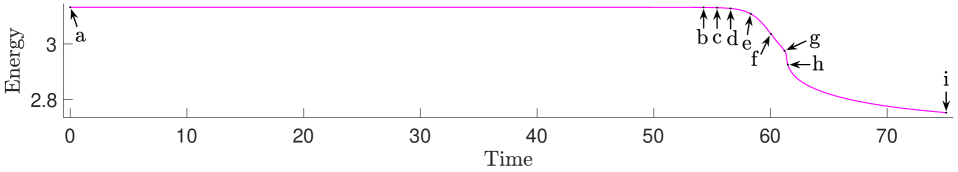
To illustrate that the oblate-like equilibria are indeed unstable against non-axisymmetric perturbations, we carry out the following two numerical experiments using the pACOK dynamics (5), with the initial values being the oblate-like equilibria that we obtained above. In the first numerical experiment, we choose $\raisebox{2.0pt}{$\widetilde{\chi}$}=1.116$ where the oblate-like equilibrium is noticeably flattened, and our goal is to demonstrate how symmetry breaking occurs. In the second numerical experiment, we choose $\raisebox{2.0pt}{$\widetilde{\chi}$}=1.004$ where the oblate-like equilibrium is very close to a ball, and our goal is to demonstrate that it is still unstable against non-axisymmetric perturbations, even when $\widetilde{\chi}$ is just slightly larger than $\raisebox{2.0pt}{$\widetilde{\chi}$}_{*}$.

The first numerical experiment is shown in Figure 4. In order to simulate the later stages (where the two fragments repel each other farther away) without the fragments reaching the boundaries of the simulation box, we carry out the simulation in a larger box $[-1/2,\,3/2]^{2}\times[0,1]$ instead of $[0,1]^{3}$. To make Figure 4 more compact, however, we use $[0,1]^{3}$ as the bounding box indicated by the straight black line segments. The first five shapes lie inside $[0,1]^{3}$, whereas the last four shapes do not. In particular, the last shape sits completely outside $[0,1]^{3}$, although this spatial relation may not be visually intuitive at first glance. When viewed from above (along the axis of revolution), the 2-D projection of such an oblate-like equilibrium tends to change from a disk to an ellipse-like shape (symmetry breaking), and eventually separate into two disconnected disk-like components.

Refer to caption

aRefer to captionRefer to captiona\overset{\includegraphics[width=58.0pt]{images/SymmetryBreaking/9/a.png}}{\begin{minipage}[t][0pt][b]{24.0pt}\hskip 7.0pta\end{minipage}} bRefer to captionRefer to captionb\overset{\includegraphics[width=58.0pt]{images/SymmetryBreaking/9/b.png}}{\begin{minipage}[t][0pt][b]{24.0pt}\hskip 7.0ptb\end{minipage}} cRefer to captionRefer to captionc\overset{\includegraphics[width=58.0pt]{images/SymmetryBreaking/9/c.png}}{\begin{minipage}[t][0pt][b]{24.0pt}\hskip 7.0ptc\end{minipage}} dRefer to captionRefer to captiond\overset{\includegraphics[width=58.0pt]{images/SymmetryBreaking/9/d.png}}{\begin{minipage}[t][0pt][b]{24.0pt}\hskip 7.0ptd\end{minipage}} eRefer to captionRefer to captione\overset{\includegraphics[width=58.0pt]{images/SymmetryBreaking/9/e.png}}{\begin{minipage}[t][0pt][b]{24.0pt}\hskip 7.0pte\end{minipage}}

fRefer to captionRefer to captionf\overset{\includegraphics[width=58.0pt]{images/SymmetryBreaking/9/f.png}}{\begin{minipage}[t][0pt][b]{24.0pt}\hskip 7.0ptf\end{minipage}} gRefer to captionRefer to captiong\overset{\includegraphics[width=58.0pt]{images/SymmetryBreaking/9/g.png}}{\begin{minipage}[t][0pt][b]{24.0pt}\hskip 7.0ptg\end{minipage}} hRefer to captionRefer to captionh\overset{\includegraphics[width=58.0pt]{images/SymmetryBreaking/9/h.png}}{\begin{minipage}[t][0pt][b]{24.0pt}\hskip 7.0pth\end{minipage}} iRefer to captionRefer to captioni\overset{\includegraphics[width=58.0pt]{images/SymmetryBreaking/9/i.png}}{\begin{minipage}[t][0pt][b]{24.0pt}\hskip 7.0pti\end{minipage}}

Figure 4: pACOK dynamics for $\raisebox{2.0pt}{$\widetilde{\chi}$}=1.116$.

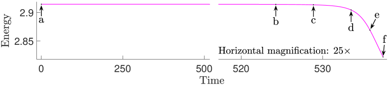
The second numerical experiment is shown in Figure 5. The simulation box is $[0,1]^{3}$, therefore we can only simulate the stages up to f, after which the shape will reach the boundaries of the simulation box. Note that the initial value (represented by a) is an oblate-like stationary point (whose axis of revolution is a vertical line) with a very tiny non-axisymmetric perturbation. After a long time, the perturbation grows exponentially large, resulting in a dramatic deformation, thus demonstrating the instability of the oblate-like equilibrium for a $\widetilde{\chi}$ that is slightly larger than $\raisebox{2.0pt}{$\widetilde{\chi}$}_{*}$.

Refer to caption

aRefer to captionRefer to captiona\overset{\includegraphics[width=58.0pt]{images/SymmetryBreaking/8.09/a.png}}{\begin{minipage}[t][0pt][b]{24.0pt}\hskip 7.0pta\end{minipage}} bRefer to captionRefer to captionb\overset{\includegraphics[width=58.0pt]{images/SymmetryBreaking/8.09/b.png}}{\begin{minipage}[t][0pt][b]{24.0pt}\hskip 7.0ptb\end{minipage}} cRefer to captionRefer to captionc\overset{\includegraphics[width=58.0pt]{images/SymmetryBreaking/8.09/c.png}}{\begin{minipage}[t][0pt][b]{24.0pt}\hskip 7.0ptc\end{minipage}} dRefer to captionRefer to captiond\overset{\includegraphics[width=58.0pt]{images/SymmetryBreaking/8.09/d.png}}{\begin{minipage}[t][0pt][b]{24.0pt}\hskip 7.0ptd\end{minipage}} eRefer to captionRefer to captione\overset{\includegraphics[width=58.0pt]{images/SymmetryBreaking/8.09/e.png}}{\begin{minipage}[t][0pt][b]{24.0pt}\hskip 7.0pte\end{minipage}} fRefer to captionRefer to captionf\overset{\includegraphics[width=58.0pt]{images/SymmetryBreaking/8.09/f.png}}{\begin{minipage}[t][0pt][b]{24.0pt}\hskip 7.0ptf\end{minipage}}

Figure 5: pACOK dynamics for $\raisebox{2.0pt}{$\widetilde{\chi}$}=1.004$.

4.2 Minimum energy paths of fission

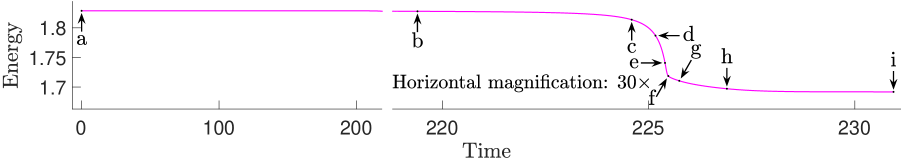
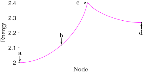
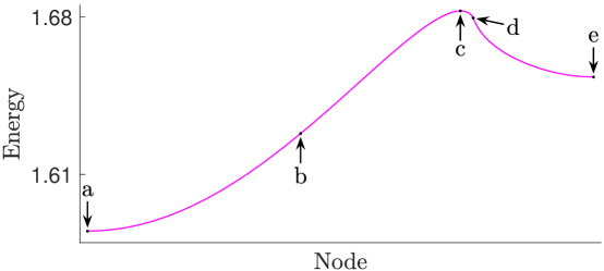
In this subsection, we obtain the minimum energy paths of fission for $\raisebox{2.0pt}{$\widetilde{\chi}$}<\raisebox{2.0pt}{$\widetilde{\chi}$}_{*}$, with the help of the string method. Complete fission paths have not been obtained in the literature before. Difficulties have been encountered in calculating the fission path near the scission point [34]. The reason we suspect is that topological changes cannot be easily handled by the sharp interface formulation in [34]. In contrast, topological changes can be easily handled in our phase-field formulation, and we are able to obtain the complete fission paths shown in Figure 6. We omit the latter part of the string where the two fragments reach the boundaries of the simulation box. The saddle points are indicated by b, c, d, e, f, g and h. The scission points are indicated by i, j, k, l, m, n and o. The details can be found in Appendix E.

Refer to caption

aRefer to captionRefer to captiona\overset{\includegraphics[width=58.0pt]{images/NoBoundary3D/3.2/a.png}}{\begin{minipage}[t][0pt][b]{24.0pt}\hskip 7.0pta\end{minipage}} bRefer to captionRefer to captionb\overset{\includegraphics[width=58.0pt]{images/NoBoundary3D/8.0/b.png}}{\begin{minipage}[t][0pt][b]{24.0pt}\hskip 7.0ptb\end{minipage}} cRefer to captionRefer to captionc\overset{\includegraphics[width=58.0pt]{images/NoBoundary3D/7.5/b.png}}{\begin{minipage}[t][0pt][b]{24.0pt}\hskip 7.0ptc\end{minipage}} dRefer to captionRefer to captiond\overset{\includegraphics[width=58.0pt]{images/NoBoundary3D/6.8/b.png}}{\begin{minipage}[t][0pt][b]{24.0pt}\hskip 7.0ptd\end{minipage}}

eRefer to captionRefer to captione\overset{\includegraphics[width=58.0pt]{images/NoBoundary3D/6.0/c.png}}{\begin{minipage}[t][0pt][b]{24.0pt}\hskip 7.0pte\end{minipage}} fRefer to captionRefer to captionf\overset{\includegraphics[width=58.0pt]{images/NoBoundary3D/5.3/c.png}}{\begin{minipage}[t][0pt][b]{24.0pt}\hskip 7.0ptf\end{minipage}} gRefer to captionRefer to captiong\overset{\includegraphics[width=58.0pt]{images/NoBoundary3D/4.7/c.png}}{\begin{minipage}[t][0pt][b]{24.0pt}\hskip 7.0ptg\end{minipage}} hRefer to captionRefer to captionh\overset{\includegraphics[width=58.0pt]{images/NoBoundary3D/3.2/c.png}}{\begin{minipage}[t][0pt][b]{24.0pt}\hskip 7.0pth\end{minipage}}

iRefer to captionRefer to captioni\overset{\includegraphics[width=58.0pt]{images/NoBoundary3D/3.2/d.png}}{\begin{minipage}[t][0pt][b]{24.0pt}\hskip 7.0pti\end{minipage}} jRefer to captionRefer to captionj\overset{\includegraphics[width=58.0pt]{images/NoBoundary3D/4.7/d.png}}{\begin{minipage}[t][0pt][b]{24.0pt}\hskip 7.0ptj\end{minipage}} kRefer to captionRefer to captionk\overset{\includegraphics[width=58.0pt]{images/NoBoundary3D/5.3/d.png}}{\begin{minipage}[t][0pt][b]{24.0pt}\hskip 7.0ptk\end{minipage}} lRefer to captionRefer to captionl\overset{\includegraphics[width=58.0pt]{images/NoBoundary3D/6.0/d.png}}{\begin{minipage}[t][0pt][b]{24.0pt}\hskip 7.0ptl\end{minipage}}

mRefer to captionRefer to captionm\overset{\includegraphics[width=58.0pt]{images/NoBoundary3D/6.8/d.png}}{\begin{minipage}[t][0pt][b]{24.0pt}\hskip 7.0ptm\end{minipage}} nRefer to captionRefer to captionn\overset{\includegraphics[width=58.0pt]{images/NoBoundary3D/7.5/d.png}}{\begin{minipage}[t][0pt][b]{24.0pt}\hskip 7.0ptn\end{minipage}} oRefer to captionRefer to captiono\overset{\includegraphics[width=58.0pt]{images/NoBoundary3D/8.0/d.png}}{\begin{minipage}[t][0pt][b]{24.0pt}\hskip 7.0pto\end{minipage}} pRefer to captionRefer to captionp\overset{\includegraphics[width=58.0pt]{images/NoBoundary3D/3.2/e.png}}{\begin{minipage}[t][0pt][b]{24.0pt}\hskip 7.0ptp\end{minipage}}

Figure 6: Minimum energy paths of fission for various fissility parameters.

As we will discuss in Section 4.3, the saddle point loses stability against mass-asymmetric perturbations when $\widetilde{\chi}$ is below a threshold $\raisebox{2.0pt}{$\widetilde{\chi}$}_{3}$. For $\raisebox{2.0pt}{$\chi$}\in(\raisebox{2.0pt}{$\chi$}_{3},\raisebox{2.0pt}{$\chi$}_{*})$, it is unknown in the physics literature if there is instability against mass-asymmetric perturbations during the descent from the saddle point to the scission point [52, Middle of Page 242]. Nix [52, Bottom of Page 265] suggested that there is likely no such instability. Our numerical results support that there is no such instability, because we are able to obtain a stable fission path for any $\raisebox{2.0pt}{$\widetilde{\chi}$}\in(\raisebox{2.0pt}{$\widetilde{\chi}$}_{3},\raisebox{2.0pt}{$\widetilde{\chi}$}_{*})$.

4.3 Businaro–Gallone point

In this subsection, we numerically verify the known results about the Businaro–Gallone point. There is a critical point $\raisebox{2.0pt}{$\widetilde{\chi}$}_{3}$ in our simulations, such that for $\raisebox{2.0pt}{$\widetilde{\chi}$}<\raisebox{2.0pt}{$\widetilde{\chi}$}_{3}$, the saddle point on the Bohr–Wheeler branch loses stability against mass-asymmetric perturbations, and thus the fission path becomes unstable. See Appendix F for another possible minimum energy path called the spallation path.

We carry out the following numerical experiment to study the instability against mass-asymmetric perturbations. First we use the shrinking dimer dynamics [71] to calculate the saddle point along the fission path for $\raisebox{2.0pt}{$\widetilde{\chi}$}\in(\raisebox{2.0pt}{$\widetilde{\chi}$}_{3},\raisebox{2.0pt}{$\widetilde{\chi}$}_{*})$. Note that we already have a good initial guess of the saddle point and its unstable direction: in our simulation results from the string method, we can use the node of the highest energy as the initial guess of the saddle point, and for the initial guess of the unstable direction we can use the difference between the top two nodes of the highest energy.

The saddle point obtained above is a stationary point on the Bohr–Wheeler branch. We can track this bifurcation branch down as $\widetilde{\chi}$ decreases. For any stationary point on the Bohr–Wheeler branch, we can make a very tiny mass-asymmetric perturbation to it and then use the perturbed shape as the initial value of the shrinking dimer dynamics. For $\raisebox{2.0pt}{$\widetilde{\chi}$}\leqslant 0.39386$, as shown in Figure 7, the shape changes very little for a long time, but then goes through a dramatic change with one end shrinking and the other growing, and eventually converges to a ball. For $\raisebox{2.0pt}{$\widetilde{\chi}$}\geqslant 0.39398$, the shape restores to equilibrium. So we know $\raisebox{2.0pt}{$\widetilde{\chi}$}_{3}\in(0.39386,0.39398)$. We use $\raisebox{2.0pt}{$\widetilde{\chi}$}_{3}/\raisebox{2.0pt}{$\widetilde{\chi}$}_{*}\approx 0.395$ to estimate $\raisebox{2.0pt}{$\chi$}_{3}$. Note that the shrinking dimer dynamics normally would not converge to a local minimizer, but our system is degenerate in the sense that there are zero eigenvalues whose eigenvectors correspond to translational motions.

Refer to caption

aRefer to captionRefer to captiona\overset{\includegraphics[width=58.0pt]{images/SymmetryBreaking/3/a.png}}{\begin{minipage}[t][0pt][b]{24.0pt}\hskip 7.0pta\end{minipage}} bRefer to captionRefer to captionb\overset{\includegraphics[width=58.0pt]{images/SymmetryBreaking/3/b.png}}{\begin{minipage}[t][0pt][b]{24.0pt}\hskip 7.0ptb\end{minipage}} cRefer to captionRefer to captionc\overset{\includegraphics[width=58.0pt]{images/SymmetryBreaking/3/c.png}}{\begin{minipage}[t][0pt][b]{24.0pt}\hskip 7.0ptc\end{minipage}} dRefer to captionRefer to captiond\overset{\includegraphics[width=58.0pt]{images/SymmetryBreaking/3/d.png}}{\begin{minipage}[t][0pt][b]{24.0pt}\hskip 7.0ptd\end{minipage}} eRefer to captionRefer to captione\overset{\includegraphics[width=58.0pt]{images/SymmetryBreaking/3/e.png}}{\begin{minipage}[t][0pt][b]{24.0pt}\hskip 7.0pte\end{minipage}}

fRefer to captionRefer to captionf\overset{\includegraphics[width=58.0pt]{images/SymmetryBreaking/3/f.png}}{\begin{minipage}[t][0pt][b]{24.0pt}\hskip 7.0ptf\end{minipage}} gRefer to captionRefer to captiong\overset{\includegraphics[width=58.0pt]{images/SymmetryBreaking/3/g.png}}{\begin{minipage}[t][0pt][b]{24.0pt}\hskip 7.0ptg\end{minipage}} hRefer to captionRefer to captionh\overset{\includegraphics[width=58.0pt]{images/SymmetryBreaking/3/h.png}}{\begin{minipage}[t][0pt][b]{24.0pt}\hskip 7.0pth\end{minipage}} iRefer to captionRefer to captioni\overset{\includegraphics[width=58.0pt]{images/SymmetryBreaking/3/i.png}}{\begin{minipage}[t][0pt][b]{24.0pt}\hskip 7.0pti\end{minipage}}

Figure 7: Shrinking dimer dynamics for $\raisebox{2.0pt}{$\widetilde{\chi}$}=0.372$.

For $\raisebox{2.0pt}{$\widetilde{\chi}$}<\raisebox{2.0pt}{$\widetilde{\chi}$}_{3}$, in order to calculate the equilibrium on the Bohr–Wheeler branch which is an index-2 saddle point, while one can use a higher-index extension of the shrinking dimer method [71, Bottom of Page 1919], we instead employ a simple technique to maintain its centrosymmetry: after every a few (e.g., 500) iterations, take the average of the computed shape and its point reflection with respect to the center of the simulation box.

4.4 Analogue in 2-D

In this subsection, we study the 2-D analogue under no boundary conditions. To the best of our knowledge, most of our results have not been seen in the literature. Note that in 2-D, a disk is only a stationary point of (1) since no global minimizer or local minimizer exists in the full space [38, Bottom of Page 78]. However, if we restrict $\Omega$ to the interior of some bounded domain in $\mathbb{R}^{2}$, then the minimizers may come into existence [4, Remark 2.14]. For brevity such restricted 2-D local minimizers are simply called local minimizers in this paper.

We numerically study the pACOK dynamics (5), with the initial value $\eta(\,\cdot\,,0)$ resembling the indicator function of a disk. According to our simulation results, there is a critical value $\raisebox{2.0pt}{$\widetilde{\chi}$}_{*}\approx 0.99978$. For any $\raisebox{2.0pt}{$\widetilde{\chi}$}>\raisebox{2.0pt}{$\widetilde{\chi}$}_{*}$, there exists a time $t>0$ such that $\eta(\,\cdot\,,t)$ is approximately the indicator function of a shape resembling an eye mask. For any $\raisebox{2.0pt}{$\widetilde{\chi}$}<\raisebox{2.0pt}{$\widetilde{\chi}$}_{*}$, we observe that $\eta(\,\cdot\,,t)$ resembles the indicator function of a disk for any $t>0$ and converges numerically to machine precision as $t\rightarrow\infty$. In other words, $\raisebox{2.0pt}{$\widetilde{\chi}$}_{*}$ is where the disk loses stability in our simulations. For the sharp interface problem (1), the critical value is known to be $\raisebox{2.0pt}{$\chi$}_{*}=1$ [58, Top of Page 1126]. The relative error between $\raisebox{2.0pt}{$\widetilde{\chi}$}_{*}$ and $\raisebox{2.0pt}{$\chi$}_{*}$ is $-0.02\%$, which could be attributed to the finitely small $c$, finitely large $K$, and finite numerical discretizations.

As mentioned above, after losing its stability, a disk will deform and converge to an eye-mask shaped local minimizer. We use such a local minimizer as the initial value, and numerically solve the pACOK dynamics (5) with a larger or smaller $\widetilde{\chi}$. In this way we can track this bifurcation branch up and down.

According to our numerical simulations, as $\widetilde{\chi}$ increases, the eye-mask shaped local minimizer becomes thinner and elongates. This persists even for $\widetilde{\chi}$ very large. When $\widetilde{\chi}$ is extremely large, the entire eye-mask shape becomes very thin especially in the middle of its neck, and its neck thickness is comparable to the diffuse interface thickness. Only then, the eye-mask shape would break up. We suspect that such a break-up is due to diffuse interface approximations, and that it would never happen in the sharp interface limit (1).

As $\widetilde{\chi}$ decreases, we observe that the eye-mask shaped local minimizer fattens and shortens. We can track this bifurcation branch all the way down to $\raisebox{2.0pt}{$\widetilde{\chi}$}=0.905$. For $\raisebox{2.0pt}{$\widetilde{\chi}$}\leqslant 0.903$, the eye-mask shape will converge to a disk. Therefore we suspect that there is a $\raisebox{2.0pt}{$\widetilde{\chi}$}_{4}\in(0.903,0.905)$ such that a saddle-node bifurcation happens at $\raisebox{2.0pt}{$\widetilde{\chi}$}_{4}$, as shown on the top-left of Figure 8.

We use the string method to obtain the minimum energy paths of fission, as shown in Figure 8 (see Appendix G for details). We omit the latter part of the string where the two fragments reach the boundaries of the simulation box. For $\raisebox{2.0pt}{$\widetilde{\chi}$}\in(\raisebox{2.0pt}{$\widetilde{\chi}$}_{4},\raisebox{2.0pt}{$\widetilde{\chi}$}_{*})$, there is an intermediate local minimizer (of an eye-mask shape, indicated by g, h, i, j and k) along the minimum energy path of fission, and there is a transition state (indicated by b, c, d, e and f) from a disk to such an intermediate local minimizer. Such a transition state resembles an ellipse for $\widetilde{\chi}$ slightly less than $\raisebox{2.0pt}{$\widetilde{\chi}$}_{*}$, and has been found by Ren and Wei in the sharp interface limit [58]. It bifurcates from a disk at $\raisebox{2.0pt}{$\widetilde{\chi}$}=\raisebox{2.0pt}{$\widetilde{\chi}$}_{*}$, and lies on a bifurcation branch which we call the Ren–Wei branch. For $\raisebox{2.0pt}{$\widetilde{\chi}$}<\raisebox{2.0pt}{$\widetilde{\chi}$}_{4}$, there is no intermediate local minimizer. The scission point (indicated by l, m, n, o, p, q and r) resembles a lemniscate and is a transition state along the minimum energy path. There is a 2-D analogue of the Businaro–Gallone point $\raisebox{2.0pt}{$\widetilde{\chi}$}_{3}\approx 0.428$, such that the critical point resembling a lemniscate becomes unstable against mass-asymmetric perturbations when $\raisebox{2.0pt}{$\widetilde{\chi}$}<\raisebox{2.0pt}{$\widetilde{\chi}$}_{3}$.

Refer to caption

aRefer to captionRefer to captiona\overset{\includegraphics[width=53.0pt]{images/NoBoundary2D/2.50/a.png}}{\begin{minipage}[t][0pt][b]{24.0pt}\hskip 10.0pta\end{minipage}} bRefer to captionRefer to captionb\overset{\includegraphics[width=53.0pt]{images/NoBoundary2D/4.69/b.png}}{\begin{minipage}[t][0pt][b]{24.0pt}\hskip 10.0ptb\end{minipage}} cRefer to captionRefer to captionc\overset{\includegraphics[width=53.0pt]{images/NoBoundary2D/4.58/b.png}}{\begin{minipage}[t][0pt][b]{24.0pt}\hskip 10.0ptc\end{minipage}} dRefer to captionRefer to captiond\overset{\includegraphics[width=53.0pt]{images/NoBoundary2D/4.47/b.png}}{\begin{minipage}[t][0pt][b]{24.0pt}\hskip 10.0ptd\end{minipage}} eRefer to captionRefer to captione\overset{\includegraphics[width=53.0pt]{images/NoBoundary2D/4.36/b.png}}{\begin{minipage}[t][0pt][b]{24.0pt}\hskip 10.0pte\end{minipage}}

fRefer to captionRefer to captionf\overset{\includegraphics[width=53.0pt]{images/NoBoundary2D/4.25/b.png}}{\begin{minipage}[t][0pt][b]{24.0pt}\hskip 10.0ptf\end{minipage}} gRefer to captionRefer to captiong\overset{\includegraphics[width=53.0pt]{images/NoBoundary2D/4.25/c.png}}{\begin{minipage}[t][0pt][b]{24.0pt}\hskip 10.0ptg\end{minipage}} hRefer to captionRefer to captionh\overset{\includegraphics[width=53.0pt]{images/NoBoundary2D/4.36/c.png}}{\begin{minipage}[t][0pt][b]{24.0pt}\hskip 10.0pth\end{minipage}} iRefer to captionRefer to captioni\overset{\includegraphics[width=53.0pt]{images/NoBoundary2D/4.47/c.png}}{\begin{minipage}[t][0pt][b]{24.0pt}\hskip 10.0pti\end{minipage}} jRefer to captionRefer to captionj\overset{\includegraphics[width=53.0pt]{images/NoBoundary2D/4.58/c.png}}{\begin{minipage}[t][0pt][b]{24.0pt}\hskip 10.0ptj\end{minipage}}

kRefer to captionRefer to captionk\overset{\includegraphics[width=53.0pt]{images/NoBoundary2D/4.69/c.png}}{\begin{minipage}[t][0pt][b]{24.0pt}\hskip 10.0ptk\end{minipage}} lRefer to captionRefer to captionl\overset{\includegraphics[width=53.0pt]{images/NoBoundary2D/4.69/d.png}}{\begin{minipage}[t][0pt][b]{24.0pt}\hskip 10.0ptl\end{minipage}} mRefer to captionRefer to captionm\overset{\includegraphics[width=53.0pt]{images/NoBoundary2D/4.58/d.png}}{\begin{minipage}[t][0pt][b]{24.0pt}\hskip 10.0ptm\end{minipage}} nRefer to captionRefer to captionn\overset{\includegraphics[width=53.0pt]{images/NoBoundary2D/4.47/d.png}}{\begin{minipage}[t][0pt][b]{24.0pt}\hskip 10.0ptn\end{minipage}} oRefer to captionRefer to captiono\overset{\includegraphics[width=53.0pt]{images/NoBoundary2D/4.36/d.png}}{\begin{minipage}[t][0pt][b]{24.0pt}\hskip 10.0pto\end{minipage}}

pRefer to captionRefer to captionp\overset{\includegraphics[width=53.0pt]{images/NoBoundary2D/4.25/d.png}}{\begin{minipage}[t][0pt][b]{24.0pt}\hskip 10.0ptp\end{minipage}} qRefer to captionRefer to captionq\overset{\includegraphics[width=53.0pt]{images/NoBoundary2D/3.50/d.png}}{\begin{minipage}[t][0pt][b]{24.0pt}\hskip 10.0ptq\end{minipage}} rRefer to captionRefer to captionr\overset{\includegraphics[width=53.0pt]{images/NoBoundary2D/2.50/d.png}}{\begin{minipage}[t][0pt][b]{24.0pt}\hskip 10.0ptr\end{minipage}} sRefer to captionRefer to captions\overset{\includegraphics[width=53.0pt]{images/NoBoundary2D/Summary/s.png}}{\begin{minipage}[t][0pt][b]{24.0pt}\hskip 10.0pts\end{minipage}} tRefer to captionRefer to captiont\overset{\includegraphics[width=53.0pt]{images/NoBoundary2D/2.50/f.png}}{\begin{minipage}[t][0pt][b]{24.0pt}\hskip 10.0ptt\end{minipage}}

Figure 8: Minimum energy paths in 2-D for various fissility parameters.

4.5 Bifurcation diagrams

The 3-D case

Our observation of the instability of the Bohr–Wheeler branch might seem surprising at first glance. The bifurcation of this branch from a ball at $\raisebox{2.0pt}{$\chi$}=\raisebox{2.0pt}{$\chi$}_{*}$ is transcritical, so we may think that its stability simply exchanges with the ball at $\raisebox{2.0pt}{$\chi$}=\raisebox{2.0pt}{$\chi$}_{*}$. In the paradigm of transcritical bifurcation, the ball is stable for $\raisebox{2.0pt}{$\chi$}<\raisebox{2.0pt}{$\chi$}_{*}$ and unstable for $\raisebox{2.0pt}{$\chi$}>\raisebox{2.0pt}{$\chi$}_{*}$, and it seems plausible that the oblate-like stationary point is stable for $\raisebox{2.0pt}{$\chi$}>\raisebox{2.0pt}{$\chi$}_{*}$, as shown on the left of Figure 9 (see also Figure 1), where the horizontal axis qualitatively represents the aspect ratio of a spheroid, i.e., the ratio of the polar radius to the equatorial radius.

If we only consider axisymmetric deformations, the above paradigm of transcritical bifurcation is qualitatively correct, because the oblate-like stationary point is indeed stable against certain axisymmetric perturbations for $\raisebox{2.0pt}{$\chi$}>\raisebox{2.0pt}{$\chi$}_{*}$ [24, Corollary 5]. However, they are unstable against non-axisymmetric perturbations according to Section 4.1. To explain this phenomenon, we need to use a 2-D transcritical bifurcation diagram.

We consider an ellipsoid which is close to a ball. It has three degrees of freedom, i.e., the lengths of its three axes. Due to the volume constraint, the degrees of freedom is reduced to two, and can be represented by the $xy$-plane on the right of Figure 9 (where the $z$-axis represents the energy). The red dot at the center represents the ball, the three yellow dots represent three prolates whose axes of revolution are perpendicular to each other, the three blue dots represent oblates, and they are all stationary points. As $\chi$ exceeds $\raisebox{2.0pt}{$\chi$}_{*}$, the three yellow dots simultaneously collide with the red dot and then convert into three blue dots. Each blue dot is stable along the direction of its motion (corresponding to axisymmetric deformations), but unstable along the perpendicular direction of its motion (corresponding to non-axisymmetric deformations).

Refer to caption
Refer to caption
Refer to caption
Figure 9: Left: typical transcritical bifurcation in 1-D. Right: a transcritical bifurcation in 2-D.

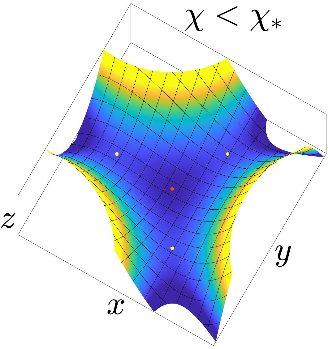
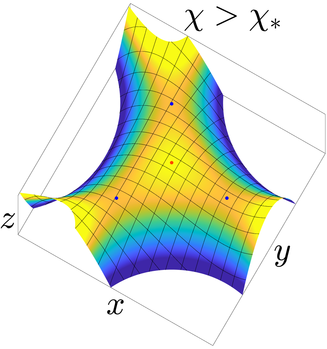
Note that Figure 9 is not produced from actual computational results but just for illustration. The left of Figure 9 is produced using a prototype transcritical bifurcation: $y=sx^{2}/2-x^{3}/3$, where $s=1$ for $\raisebox{2.0pt}{$\chi$}<\raisebox{2.0pt}{$\chi$}_{*}$, and $s=-1$ for $\raisebox{2.0pt}{$\chi$}>\raisebox{2.0pt}{$\chi$}_{*}$. The right of Figure 9 is produced by constructing three transcritical bifurcations along different directions colliding simultaneously, i.e., $z=sr^{2}/2+\cos(3\theta)\,r^{3}/3$, where $s=0.85$ for $\raisebox{2.0pt}{$\chi$}<\raisebox{2.0pt}{$\chi$}_{*}$, $s=-0.85$ for $\raisebox{2.0pt}{$\chi$}>\raisebox{2.0pt}{$\chi$}_{*}$, and $(r,\theta)$ is $(x,y)$ in polar coordinates. It has been noticed in the literature [16, Caption of Figure 39] that the instability of the oblate-like stationary points may be attributed to identically deformed but differently oriented bifurcation branches colliding simultaneously. The right of our Figure 9 provides a concrete example for visual illustration.

The 2-D case

The situation in 2-D is a little different, because a 3-D prolate and oblate have no analogues in 2-D (they both correspond to ellipses which cannot be distinguished like a prolate and oblate). As a result, the bifurcation in 2-D at $\raisebox{2.0pt}{$\chi$}=\raisebox{2.0pt}{$\chi$}_{*}$ is not transcritical but of a pitchfork type (in a generalized sense, see [58, Page 1127]). It can be either supercritical or subcritical. Ren and Wei proposed the following conjecture [58, Observation 1.1, Hypothesis 3.2, and Section 6]:

Conjecture 4.1.

The bifurcation at $\raisebox{2.0pt}{$\chi$}=\raisebox{2.0pt}{$\chi$}_{*}$ is of the supercritical pitchfork type. The equilibrium on this bifurcation branch (what we call the Ren–Wei branch) given by [58, Equation (3.7)], only exists for $\raisebox{2.0pt}{$\chi$}>\raisebox{2.0pt}{$\chi$}_{*}$, and is stable.

If the above conjecture is true, a disk, after losing its stability (for $\chi$ slightly larger than $\raisebox{2.0pt}{$\chi$}_{*}$), would deform into a local minimizer resembling an ellipse, whose eccentricity increases with $\chi$. This scenario can be qualitatively illustrated by Figure 10-(b), where the points $A$ and $B$ represent ellipse-like local minimizers, $O$ represents the disk, and $s$ qualitatively represents $\raisebox{2.0pt}{$\chi$}-\raisebox{2.0pt}{$\chi$}_{*}$. Therefore Ren and Wei suggested a saturation process depicted in Figure 10-(a), where the word saturation refers to the process of a disk splitting into two disks as $\chi$ increases. They believed that the local minimizer will no longer be a disk but resemble an ellipse after $\chi$ exceeds $\raisebox{2.0pt}{$\chi$}_{*}$, then a neck will appear for some larger $\chi$, and finally it will break into two disconnected disks for $\chi$ large enough [58, Page 1120].

However, for $\raisebox{2.0pt}{$\chi$}>\raisebox{2.0pt}{$\chi$}_{*}$ we have not numerically found a stable equilibrium resembling an ellipse. In fact, as mentioned in Section 4.4, a disk after becoming unstable will eventually deform into a local minimizer resembling an eye mask, instead of settling into an ellipse-like equilibrium. For $\raisebox{2.0pt}{$\chi$}<\raisebox{2.0pt}{$\chi$}_{*}$, we are able to numerically find unstable equilibria resembling ellipses (represented by b and c in Figure 8). Therefore our numerical results suggest the scenario illustrated by Figure 10-(c), where the points $B$, $D$ and $E$ represent eye-mask shaped local minimizers, $A$ and $C$ represent ellipse-like saddle points, $O$ represents the disk, and $s$ qualitatively represents $\raisebox{2.0pt}{$\chi$}_{*}-\raisebox{2.0pt}{$\chi$}$. In other words, we believe that Conjecture 4.1 is false, and we propose the following conjecture:

Conjecture 4.2.

The bifurcation at $\raisebox{2.0pt}{$\chi$}=\raisebox{2.0pt}{$\chi$}_{*}$ is of the subcritical pitchfork type. The equilibrium on the Ren–Wei branch only exists for $\raisebox{2.0pt}{$\chi$}<\raisebox{2.0pt}{$\chi$}_{*}$, and is unstable.

(a) Refer to caption

Refer to caption

(b)                                                   (c)

Figure 10: (a) Saturation process in the supercritical scenario (Figure from [58, Figure 1]. Copyright ©2009 Society for Industrial and Applied Mathematics. Reprinted with permission. All rights reserved). (b) Supercritical scenario. (c) Subcritical scenario.

Figure 10-(b) is produced using a prototype supercritical pitchfork bifurcation, i.e., $y=x^{4}-2sx^{2}$. Figure 10-(c) is produced using $y=x^{6}/3-x^{4}+sx^{2}$. Neither of them is produced from actual computational results, and they are both for illustration only.

5 Periodic isoperimetric problem: resistance to rupture

As noted in the literature [43, Page 6], the underlying reason for the rupture of one nucleus into two nuclei is the Plateau–Rayleigh instability, which explains the rupture of a long thin liquid cylinder into many droplets due to surface tension. This is why a thin fiber of water is rarely observed, while a thin film of water can be observed sometimes (e.g., on a bubble). According to Appendix C, a lamella is always a stable equilibrium.

From the results in Section 4, we notice a difference in the fission process between 2-D and 3-D. In 2-D, the rupture requires energy inputs, because the scission point is always a transition state. In 3-D, however, the scission point is never a transition state, and the rupture is energetically spontaneous (following the energy descent direction).

To explain such a difference from the viewpoint of the Plateau–Rayleigh instability, we demonstrate the roles that surface tension and dimensionality play, and focus on the cases where only the surface energy is present. In all simulations throughout this section, we choose $\raisebox{2.0pt}{$\widetilde{\chi}$}=0$ and numerically calculate the minimum energy paths involving topological changes. The problem under study in this section is the periodic isoperimetric problem and its diffuse interface version, which have been considered in [15, Equations (3.9) and (3.10)].

5.1 The 2-D case

With a fixed volume fraction $\omega=(4\pi\!-\!3\sqrt{3})/18\approx 0.4095$, we use the string method to compute a minimum energy path between two local minimizers: from a strip to a disk. Note that our 2-D simulation can be regarded as a cross section of a 3-D simulation (by a trivial extension along the third dimension), corresponding to a path from a lamella to a cylinder. For disambiguation, we use the convention that a lamella is 3-D while a strip is 2-D.

As shown in Figure 11, along the minimum energy path, the scission point c is the transition state. It resembles two arcs intersecting at a single point. Intuitively, the shape of the scission point is away from a disk, so the surface tension is trying to induce a rupture into left and right halves; however, the connection of the two halves at a single point is strong enough to resist the tendency to rupture. Therefore, the shape stays in a stalemate. This phenomenon is similar to what we have seen from the minimum energy paths presented in Section 4.4 where $\raisebox{2.0pt}{$\widetilde{\chi}$}>0$.

Refer to caption

aRefer to captionRefer to captiona\overset{\includegraphics[width=53.0pt]{images/Classical2D/a.png}}{\begin{minipage}[t][0pt][b]{24.0pt}\hskip 10.0pta\end{minipage}}     bRefer to captionRefer to captionb\overset{\includegraphics[width=53.0pt]{images/Classical2D/b.png}}{\begin{minipage}[t][0pt][b]{24.0pt}\hskip 10.0ptb\end{minipage}}

cRefer to captionRefer to captionc\overset{\includegraphics[width=53.0pt]{images/Classical2D/c.png}}{\begin{minipage}[t][0pt][b]{24.0pt}\hskip 10.0ptc\end{minipage}}     dRefer to captionRefer to captiond\overset{\includegraphics[width=53.0pt]{images/Classical2D/d.png}}{\begin{minipage}[t][0pt][b]{24.0pt}\hskip 10.0ptd\end{minipage}}

Figure 11: Minimum energy path from a strip to a disk.

In the sharp interface limit, the minimum energy path in Figure 11 should follow the trajectory of a volume preserving mean curvature flow (with the arc length corresponding to a reparametrization of the time variable). The sharp interface counterpart of the transition state c, if satisfying the Euler–Lagrange equation (7) almost everywhere, must have circular boundaries. Therefore we propose the following conjecture:

Conjecture 5.1.

With a fixed volume fraction $\omega$, as $c\rightarrow 0$ and $K\rightarrow\infty$, the transition state (represented by c in Figure 11) from a strip to a disk, converges in $L^{2}$ to the indicator function of a symmetric lens, which is formed by two intersecting circles of equal radii $R$.

After a simple calculation, we can obtain the precise shape of the transition state.

Proposition 5.2.

If Conjecture 5.1 is true, as $\omega$ increases from 0 to $\pi/4$, the radius $R$ decreases from $\infty$ to $1/2$, as determined by $\omega=2R^{2}\arcsin\big(1/(2R)\big{missing})-\sqrt{R^{2}\!-\!1/4}$. In particular, when $\omega=(4\pi\!-\!3\sqrt{3})/18\approx 0.4095$, we have $R=1/\sqrt{3}$, and thus the transition state is of the shape of the vesica piscis.

5.2 The 3-D case

For $\omega=0.09$, $0.15$ and $0.2$, we use the string method to compute a minimum energy path between two local minimizers: from a cylinder to a ball, as shown in Figures 12, 13 and 14, respectively. We can see that the scission point, represented by c, d and d in the three Figures, respectively, is never a transition state. Intuitively, in 3-D, the connection of the top and bottom halves at a single point is not strong enough to resist the tendency to rupture.

Refer to caption aRefer to captionRefer to captiona\overset{\includegraphics[width=58.0pt]{images/Classical3D/V=0.09/a.png}}{\begin{minipage}[t][0pt][b]{24.0pt}\hskip 7.0pta\end{minipage}} bRefer to captionRefer to captionb\overset{\includegraphics[width=58.0pt]{images/Classical3D/V=0.09/b.png}}{\begin{minipage}[t][0pt][b]{24.0pt}\hskip 7.0ptb\end{minipage}} cRefer to captionRefer to captionc\overset{\includegraphics[width=58.0pt]{images/Classical3D/V=0.09/c.png}}{\begin{minipage}[t][0pt][b]{24.0pt}\hskip 7.0ptc\end{minipage}} dRefer to captionRefer to captiond\overset{\includegraphics[width=58.0pt]{images/Classical3D/V=0.09/d.png}}{\begin{minipage}[t][0pt][b]{24.0pt}\hskip 7.0ptd\end{minipage}} eRefer to captionRefer to captione\overset{\includegraphics[width=58.0pt]{images/Classical3D/V=0.09/e.png}}{\begin{minipage}[t][0pt][b]{24.0pt}\hskip 7.0pte\end{minipage}}

Figure 12: Minimum energy path from a cylinder to a ball for $\omega=0.09$

Refer to caption aRefer to captionRefer to captiona\overset{\includegraphics[width=58.0pt]{images/Classical3D/V=0.15/a.png}}{\begin{minipage}[t][0pt][b]{24.0pt}\hskip 7.0pta\end{minipage}} bRefer to captionRefer to captionb\overset{\includegraphics[width=58.0pt]{images/Classical3D/V=0.15/b.png}}{\begin{minipage}[t][0pt][b]{24.0pt}\hskip 7.0ptb\end{minipage}} cRefer to captionRefer to captionc\overset{\includegraphics[width=58.0pt]{images/Classical3D/V=0.15/c.png}}{\begin{minipage}[t][0pt][b]{24.0pt}\hskip 7.0ptc\end{minipage}} dRefer to captionRefer to captiond\overset{\includegraphics[width=58.0pt]{images/Classical3D/V=0.15/d.png}}{\begin{minipage}[t][0pt][b]{24.0pt}\hskip 7.0ptd\end{minipage}} eRefer to captionRefer to captione\overset{\includegraphics[width=58.0pt]{images/Classical3D/V=0.15/e.png}}{\begin{minipage}[t][0pt][b]{24.0pt}\hskip 7.0pte\end{minipage}}

Figure 13: Minimum energy path from a cylinder to a ball for $\omega=0.15$

Refer to caption aRefer to captionRefer to captiona\overset{\includegraphics[width=58.0pt]{images/Classical3D/V=0.2/a.png}}{\begin{minipage}[t][0pt][b]{24.0pt}\hskip 7.0pta\end{minipage}} bRefer to captionRefer to captionb\overset{\includegraphics[width=58.0pt]{images/Classical3D/V=0.2/b.png}}{\begin{minipage}[t][0pt][b]{24.0pt}\hskip 7.0ptb\end{minipage}} cRefer to captionRefer to captionc\overset{\includegraphics[width=58.0pt]{images/Classical3D/V=0.2/c.png}}{\begin{minipage}[t][0pt][b]{24.0pt}\hskip 7.0ptc\end{minipage}} dRefer to captionRefer to captiond\overset{\includegraphics[width=58.0pt]{images/Classical3D/V=0.2/d.png}}{\begin{minipage}[t][0pt][b]{24.0pt}\hskip 7.0ptd\end{minipage}} eRefer to captionRefer to captione\overset{\includegraphics[width=58.0pt]{images/Classical3D/V=0.2/e.png}}{\begin{minipage}[t][0pt][b]{24.0pt}\hskip 7.0pte\end{minipage}}

Figure 14: Minimum energy path from a cylinder to a ball for $\omega=0.2$

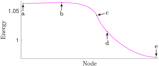
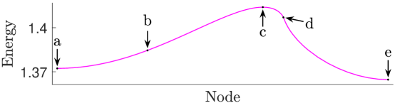
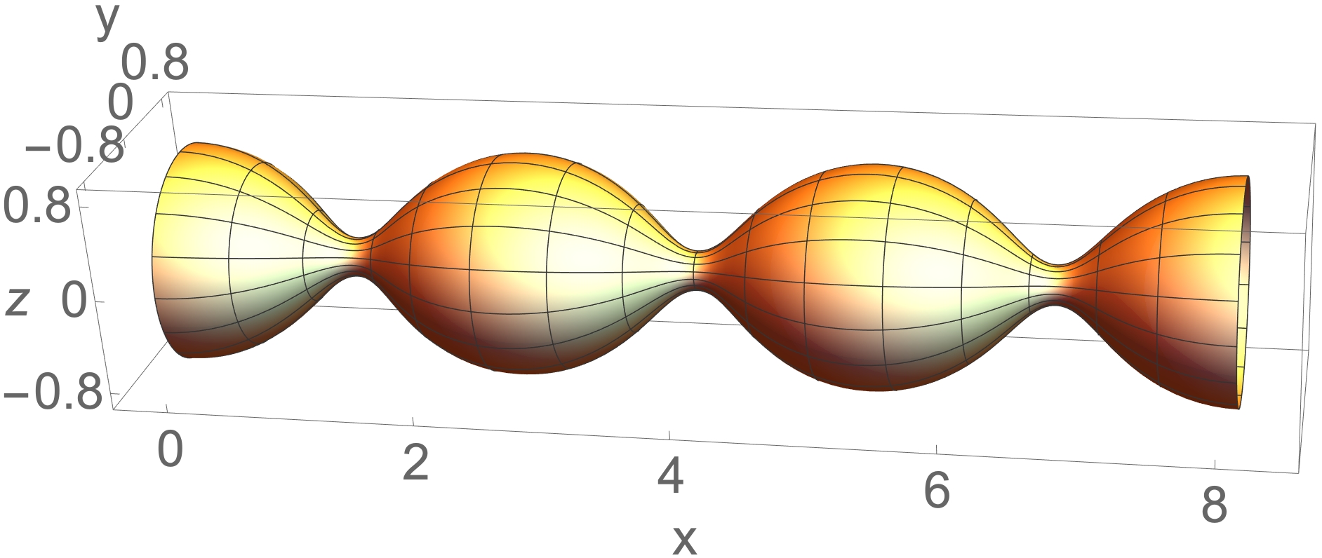
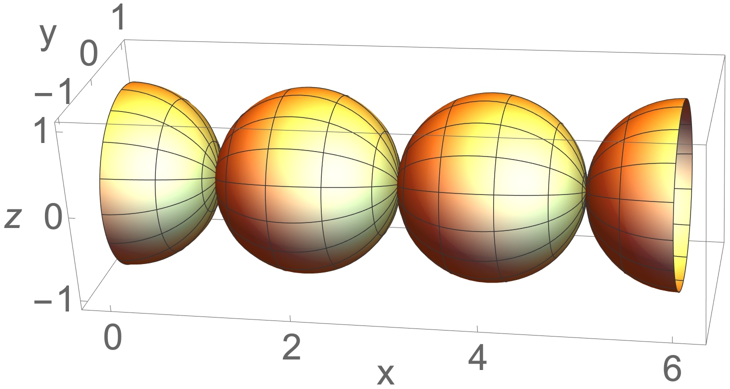
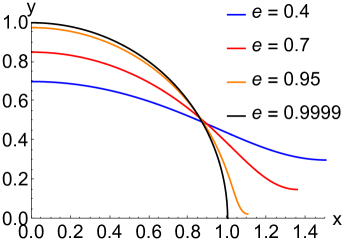
The transition state, represented by b, c and c in Figures 12, 13 and 14, respectively, resembles the interior of an unduloid. Unduloids [31] are a family of constant mean curvature surfaces of revolution, whose meridians are obtained by tracing a focus of an ellipse rolling without slippage along the axis of revolution. The eccentricity $e$ of an unduloid refers to the eccentricity of the rolling ellipse. As $e\rightarrow 0$, the unduloid converges to a cylinder; as $e\rightarrow 1$, the unduloid converges to a series of balls, with its neck circumference shrinking to 0, as shown in Figure 15.

Refer to caption
Refer to caption
Figure 15: Three periods of unduloids: $e=0.7$ (left) and $e=0.9999$ (right).
Conjecture 5.3.

With a fixed volume fraction $\omega\in\big{(}(4\pi)^{-1},\pi/6\big{)}$, as $c\rightarrow 0$ and $K\rightarrow\infty$, the transition state (represented by b, c and c in Figures 12, 13 and 14, respectively) from a cylinder to a ball, converges in $L^{2}$ to the indicator function of an unduloid. As $\omega$ increases from $(4\pi)^{-1}$ to $\pi/6$, the eccentricity $e$ increases from 00 to $1$.

Remark 5.4.

When $\omega<(4\pi)^{-1}\approx 0.08$, the unduloid disappears, through what we believe is a subcritical pitchfork bifurcation, and the cylinder becomes unstable (the Plateau–Rayleigh instability). Note that a cylinder is stable if and only if its height is less than its circumference, see [53, § 396 – § 401] and [63, Appendix I]. According to the isoperimetric inequality, a disk and a ball are always stable. A strip and a lamella are also always stable according to Appendix C.

6 Asymptotic analysis: two touching balls or disks

As shown in Figure 2, Sections 4.2 and 4.4, when $\widetilde{\chi}$ is small, the transition state in 3-D seems to have a thin neck, while the transition state in 2-D seems to be non-smooth and form an angle in the middle. In Section 5, we observe similar phenomena for $\raisebox{2.0pt}{$\widetilde{\chi}$}=0$. To gain more insight into such a difference between 2-D and 3-D, in this section we consider the cases for $\raisebox{2.0pt}{$\chi$}\ll 1$ using asymptotic analysis.

In 3-D, the following conjecture is stated in [24, Middle of Page 071506-2].

Conjecture 6.1.

The Bohr–Wheeler branch in 3-D continues to arbitrarily small $\chi$, and the saddle point on this branch converges to two touching balls in the limit of $\raisebox{2.0pt}{$\chi$}\rightarrow 0$.

As shown in Figure 2, our numerical results indicate that Conjecture 6.1 is correct. We perform asymptotic analysis and obtain the following result.

Theorem 6.2.

If Conjecture 6.1 is true, the neck circumference of the saddle point on the Bohr–Wheeler branch is $\sqrt[3]{3|\Omega|/(8\pi)}5\raisebox{2.0pt}{$\chi$}\pi/3+\sqrt[3]{|\Omega|}o(\raisebox{2.0pt}{$\chi$})$ for $\raisebox{2.0pt}{$\chi$}\ll 1$.

In 2-D, we propose the following conjectures based on our numerical results in Section 4.4.

Conjecture 6.3.

The Ren–Wei branch in 2-D does not continue to arbitrarily small $\chi$, and it disappears at $\raisebox{2.0pt}{$\chi$}=\raisebox{2.0pt}{$\chi$}_{4}\approx 0.904\pm 0.001$ through a saddle-node bifurcation. As $\chi$ decreases from $\raisebox{2.0pt}{$\chi$}_{*}$ to $\raisebox{2.0pt}{$\chi$}_{4}$, the equilibrium on this branch changes its shape from a disk to an ellipse-like shape to an eye mask.

Conjecture 6.4.

There is a separate branch consisting of the scission points. Each scission point resembles a lemniscate and is a transition state for $\raisebox{2.0pt}{$\chi$}>\raisebox{2.0pt}{$\chi$}_{3}$, where $\raisebox{2.0pt}{$\chi$}_{3}\approx 0.428$ is the 2-D analogue of the Businaro–Gallone point. For $\raisebox{2.0pt}{$\chi$}<\raisebox{2.0pt}{$\chi$}_{3}$, the scission point becomes unstable against mass-asymmetric perturbations, but the branch continues to arbitrarily small $\chi$, and the scission point on this branch converges to two touching disks as $\raisebox{2.0pt}{$\chi$}\rightarrow 0$.

We perform asymptotic analysis and obtain the following result.

Theorem 6.5.

If Conjecture 6.4 is true, the angle formed by the lemniscate-like scission point is $3\raisebox{2.0pt}{$\chi$}\pi/\sqrt{8}+o(\raisebox{2.0pt}{$\chi$})$ for $\raisebox{2.0pt}{$\chi$}\ll 1$.

Proof. [of Theorem 6.5] Consider the energy functional (4). We study its critical point configuration that is close to two touching disks when $\gamma\ll 1$. We expect such a critical point to satisfy the Euler–Lagrange equation (7) almost everywhere. When $\gamma=0$, obviously (7) is satisfied almost everywhere by two perfect disks touching at a single point. For $0<\gamma\ll 1$, we have the following intuition: the potential $\phi$ is higher at the center where the two disk-like components touch each other, and thus the curvature $H$ is smaller there, so an angle must be formed by the intersecting interfaces. We want to determine the angle asymptotically.
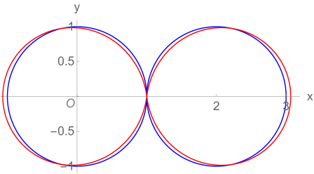
Fix $|\Omega|$ to be $2\pi$, then in the limit of $\gamma=0$, the radius of each disk is 1, as described by $\rho(\theta)=1$ for $\theta\in[0,2\pi)$ in polar coordinates (corresponding to the black circles in Figure 16). For $0<\gamma\ll 1$, we expect the critical point configuration to be slightly perturbed, as described by $\rho(\theta)=1+\varepsilon p(\theta)$, with $0<\varepsilon\ll 1$ and $p\in C^{2}[0,2\pi]$ (corresponding to the red curves in Figure 16). We assume that $p$ is symmetric, i.e., $p(\theta)=p(2\pi-\theta)$. We can also require $p(0)=0$. Note that $p$ describes the deformation of the left half, and that the right half goes through a symmetric deformation.

$\theta$ $O$ $T$ $1\!\!+\!\varepsilon p(\theta)$ $1$
Figure 16: Perturbation of two touching disks. Black: perfect disks. Red: perturbed disks.

Under mass-symmetric assumptions, the area of the left half is $\pi$, i.e.,

$$\pi=\frac{1}{2}\int_{0}^{2\pi}\rho^{2}(\theta)\differential{\theta}=\pi+\varepsilon\int_{0}^{2\pi}p(\theta)\differential{\theta}+o(\varepsilon),$$

therefore we require $\int_{0}^{2\pi}p(\theta)\differential{\theta}=0$.

The curvature $H$ is given by

$$H=\frac{2\rho^{\prime 2}+\rho^{2}-\rho\rho^{\prime\prime}}{(\rho^{\prime 2}+\rho^{2})^{3/2}}=1-(p+p^{\prime\prime})\varepsilon+o(\varepsilon).$$

When $\varepsilon\ll 1$, we expect $\Omega$ to be very close to two perfect disks. Hence, we expect

$$\phi(\theta)=\frac{\ln(5\!-\!4\cos\theta)}{-4\pi}\pi+o(1),$$

where $\phi(\theta)$ denotes the potential $\phi$ evaluated at $\big{(}\rho(\theta),\theta\big{)}$ in polar coordinates.

According to (7), we have

$$1-(p+p^{\prime\prime})\varepsilon+o(\varepsilon)+\gamma\frac{\ln(5\!-\!4\cos\theta)}{-4}+\gamma\,o(1)=\lambda,$$

therefore we know that $\varepsilon$ and $\gamma$ are of the same order, and without loss of generality, we assume $\varepsilon=\gamma$. Equating the first-order terms in the above equation, we obtain

$$p(\theta)+p^{\prime\prime}(\theta)+\frac{\ln(5\!-\!4\cos\theta)}{4}=\text{constant},$$ (9)

where the constant is independent of $\theta$, and arises from the fact that $\lambda$ may be dependent on $\varepsilon$. Using WOLFRAM MATHEMATICA, we obtain a solution satisfying (9) as well as all the other conditions that we have imposed:

$$16p(\theta)=6\arccot\big(3\tan(\theta/2)\big{missing})\sin\theta+(6\!+\!8\ln 2)(1\!-\!\cos\theta)+5(\theta\!-\!\pi)\sin\theta+(5\cos\theta\!-\!4)\ln(5\!-\!4\cos\theta),$$

with the constant in (9) adopting the value $(1\!+\!4\ln 2)/8$. As shown in Figure 17, since $\partial_{+}p(0)=-\pi/8$ and $\partial_{-}p(2\pi)=\pi/8$, we know that the angle formed by the tangent lines is $\varepsilon\pi/4+o(\varepsilon)$. By (4) we have $\varepsilon=\gamma=12\raisebox{2.0pt}{$\chi$}(2\pi/\pi)^{-3/2}$, so the angle is $3\raisebox{2.0pt}{$\chi$}\pi/\sqrt{8}$ asymptotically.

Refer to caption
Figure 17: Blue: $\rho=1$ and its mirror image. Red: $\rho=1+p/\pi$ and its mirror image.

Proof. [of Theorem 6.2] When $\gamma=0$, the Euler–Lagrange equation (7) is satisfied almost everywhere by two perfect balls touching at a single point. For $0<\gamma\ll 1$, we have the following intuition: the potential $\phi$ is higher at the center where the two ball-like components are connected, and thus the mean curvature $H$ is smaller there, so naturally we expect a cone or a neck to be formed. However, there cannot be a cone-like structure connecting the two ball-like components, because the mean curvature of a cone is very large near its apex. Instead, it is reasonable to have a neck there, resembling the neck of an unduloid, because $\phi$ and thus $H$ are almost constant there (their gradients vanish due to symmetry). We want to determine the neck circumference asymptotically.

We assume that the equilibrium is axisymmetric. In Figure 18, we make no assumption on the existence of a neck, and still use a similar parameterization as in the Proof of Theorem 6.5 (the 2-D case), i.e., we let $\rho(\theta)=1+\varepsilon p(\theta)$, but no longer require $p(0)=0$. We require $p(\pi)=0$ instead, and assume that $p$ is symmetric, i.e., $p(\theta)=p(2\pi-\theta)$.

$\theta$ $O$ $1\!\!+\!\varepsilon p(\theta)$ $1$
Figure 18: Meridians of two touching balls. Black: perfect balls. Red: perturbed balls.

The mean curvature $H$ is given by [30, Equation (15.13)]

$$H=\frac{x^{\prime}y^{\prime\prime}-x^{\prime\prime}y^{\prime}}{2\left(x^{\prime 2}+y^{\prime 2}\right)^{3/2}}-\frac{x^{\prime}/y}{2\sqrt{x^{\prime 2}+y^{\prime 2}}},$$

where $x(\theta)=\rho(\theta)\cos(\theta)$ and $y(\theta)=\rho(\theta)\sin(\theta)$. For $\rho=1+\varepsilon p$ and $\varepsilon\ll 1$, we have

$$H=1-\frac{\varepsilon}{2}\big{(}p^{\prime\prime}(\theta)+p^{\prime}(\theta)\cot\theta+2p(\theta)\big{)}+o(\varepsilon).$$

Under the volume constraints and mass-symmetric assumptions, the volume of the left half is fixed to be $4\pi/3$, that is

$$\frac{4\pi}{3}=\bigg{|}\pi\int_{0}^{\pi}y^{2}x^{\prime}\differential{\theta}\bigg{|}=\frac{4\pi}{3}+\pi\varepsilon\int_{0}^{\pi}\big{(}3p(\theta)\sin\theta-p^{\prime}(\theta)\cos\theta\big{)}\sin^{2}\theta\differential{\theta}+o(\varepsilon).$$

Therefore we require $\int_{0}^{\pi}\big{(}3p(\theta)\sin\theta-p^{\prime}(\theta)\cos\theta\big{)}\sin^{2}\theta\differential{\theta}=0$.

For $\varepsilon\ll 1$, we expect $\Omega$ to be very close to two perfect balls touching each other at a single point. Hence, we expect

$$\phi(\theta)=\Big{(}4\pi\sqrt{5\!-\!4\cos\theta}\Big{)}^{-1}\frac{4\pi}{3}+(4\pi)^{-1}\frac{4\pi}{3}+o(1).$$

According to (7), we have

$$2-\varepsilon\big{(}p^{\prime\prime}(\theta)+p^{\prime}(\theta)\cot\theta+2p(\theta)\big{)}+o(\varepsilon)+\frac{\gamma}{3}\Big{(}\sqrt{5\!-\!4\cos\theta}\Big{)}^{-1}+\frac{\gamma}{3}+\gamma\,o(1)=\lambda.$$

As before, by letting $\varepsilon=\gamma$ and equating the first-order terms in the above equation, we obtain

$$p^{\prime\prime}(\theta)+p^{\prime}(\theta)\cot\theta+2p(\theta)=\Big{(}3\sqrt{5\!-\!4\cos\theta}\Big{)}^{-1}+\text{constant}.$$

With the help of WOLFRAM MATHEMATICA, we obtain a solution, with the constant on the above right-hand side adopting the value $-5/36$,

$\displaystyle 72p(\theta)=$  $\displaystyle\;10\sqrt{5\!-\!4\cos\theta}-23+\Big{(}\,7+6\ln(4/27)-2\ln(1\!-\!\cos\theta)$ (10)
$\displaystyle+18\ln\big(\sqrt{5\!-\!4\cos\theta}\!+\!3\big{missing})-14\ln\big(\sqrt{5\!-\!4\cos\theta}\!+\!1\big{missing})\,\Big{)}\cos\theta.$

Figure 19 visualizes the deformation. The singularity of $p$ indicates the formation of a neck near $(x,y)=(1,0)$. As mentioned earlier, near the neck, $\phi$ and thus $H$ are almost constant, so the neck should resemble the neck of an unduloid.

Refer to caption
Figure 19: Blue: $\rho=1$ and its mirror image. Red: $\rho=1+15p/\pi$.

As shown in Figure 15, unduloids are surfaces of revolution with constant mean curvature. The meridians of unduloids (whose mean curvature is always 1) are parameterized by [31, Theorem 3.1]

$$x(u)=\frac{1\!-\!e}{2}F\left(\frac{u}{2},\frac{2\sqrt{e}}{1\!+\!e}\right)+\frac{1\!+\!e}{2}E\left(\frac{u}{2},\frac{2\sqrt{e}}{1\!+\!e}\right),\quad y(u)=\sqrt{1+2e\cos u+e^{2}}\big{/}2,\quad u\in[0,2\pi],$$

where $e\in(0,1)$ is the eccentricity, $F(\,\cdot\,,\,\cdot\,)$ and $E(\,\cdot\,,\,\cdot\,)$ are the incomplete elliptic integral of the first and second kinds, respectively.

Refer to caption
Figure 20: Meridians of half periods of unduloids.

As shown in Figure 20, the meridian converges to a limiting curve $x=\sqrt{1\!-\!y^{2}}$ as $e\rightarrow 1$. For $e\approx 1$, we consider the deviation of the meridian from the limiting curve and then compare it to (10). To this end, we eliminate $u$ using $u=\arccos\big((4y^{2}\!-\!1\!-\!e^{2})/(2e)\big{missing})$, and then compute the Taylor expansion of $x(y)$ at $e=1$ as follows,

$$x=\sqrt{1\!-\!y^{2}}+\frac{e\!-\!1}{2}\Big{(}\sec\theta-\ln\cot\frac{\theta}{2}\Big{)}+o(1\!-\!e),$$

where $\theta=\arcsin y$. Write $\rho=\sqrt{x^{2}+y^{2}}$, we have

$$\rho=1+\frac{e\!-\!1}{2}\Big{(}1-\cos\theta\ln\cot\frac{\theta}{2}\Big{)}+o(1\!-\!e),$$ (11)

where $\ln\cot(\theta/2)=-\ln\theta+\ln 2+O\big{(}\theta^{2}\big{)}$.

In order to obtain the relation between $e$ and $\varepsilon$, we compare (11) to $\rho=1+\varepsilon p(\theta)$ (with $p$ defined in (10)), up to leading-order terms. Noticing that in (10), we have $\ln(1\!-\!\cos\theta)=2\ln\theta-\ln 2+O\big{(}\theta^{2}\big{)}$. We want to match the following two leading order terms

$$1+\frac{e\!-\!1}{2}\cos\theta\ln\theta\quad\text{and}\quad 1+\varepsilon\frac{-2\cos\theta}{72}2\ln\theta,$$

therefore we obtain $\varepsilon=9(1\!-\!e)$.

Note that the minimum of $y(u)$ is attained at $y(\pi)=(1\!-\!e)/2$, so the neck circumference is $2\pi(1\!-\!e)/2=\varepsilon\pi/9$. According to (4), we have

$$\varepsilon=\gamma=\frac{40\pi\raisebox{2.0pt}{$\chi$}}{2(4\pi/3)}=15\raisebox{2.0pt}{$\chi$}.$$

Now that we know the neck circumference is asymptotically $5\raisebox{2.0pt}{$\chi$}\pi/3$ under the volume constraint $|\Omega|=2(4\pi/3)$, by rescaling we know that the neck circumference is asymptotically $\sqrt[3]{3|\Omega|/(8\pi)}5\raisebox{2.0pt}{$\chi$}\pi/3$ under an arbitrary volume constraint. ∎

7 Discussion

In the literature (e.g., [72, Figure 3]), it has been noticed that as $\chi$ increases, the energy minimizer changes from one ball to a few balls to many balls (or disks in the 2-D case). For $\chi$ sufficiently large, the minimizer resembles many periodically arranged tiny balls (or disks) of roughly equal sizes [13, 41]. In the context of pattern formation, this is called a saturation process from a coarse structure to a fine structure, and is not well understood mathematically [58, Page 1120]. The present work sheds light on how a ball (or disk) loses stability. We have shown that the saturation process is hysteretic, because when $\chi$ slightly exceeds the threshold $\raisebox{2.0pt}{$\chi$}_{*}$, a ball (or disk) will destabilize and eventually go through a dramatic change over a long period of time, after which even if $\chi$ falls back below $\raisebox{2.0pt}{$\chi$}_{*}$, the shape will not be restored to a ball (or disk). More specifically, our numerical results show that the oblate-like stationary points are unstable with respect to non-axisymmetric perturbations, and that the pitchfork bifurcation from a disk is subcritical instead of supercritical. But it remains open to analytically prove that the oblate-like stationary points are indeed unstable, and that the pitchfork bifurcation from a disk is indeed subcritical. As a side note, in some other systems such as a rotating liquid drop with no charge or a rotating self-gravitating celestial object [5, 64], similar phenomena occur [32, Figure 4.9].

For $\raisebox{2.0pt}{$\chi$}>\raisebox{2.0pt}{$\chi$}_{3}$, there is a Businaro–Gallone branch consisting of mass-asymmetric saddle points which are of index 2 [16, Page 144]. Nix as well as Strutinskiĭ [52, Middle of Page 251] was able to track this branch for $\raisebox{2.0pt}{$\chi$}\in(\raisebox{2.0pt}{$\chi$}_{3},0.80)$; for $\raisebox{2.0pt}{$\chi$}>0.80$, the fate of this family is unknown but of great interest. It will be interesting and promising to use our phase-field approach together with a higher-index extension of the shrinking dimer method [71, Bottom of Page 1919] to search for such index-2 saddle points for $\raisebox{2.0pt}{$\chi$}>0.80$.

In the present work, we have only considered the simplest liquid drop model. To more accurately describe atomic nuclei, the liquid drop model would need some corrections. It is likely that one could adapt our method to handle more complicated modified versions of the liquid drop model. For example, we may add a rotational energy term to handle angular momenta [43, Page 6], or add a surface curvature energy term [35, Equation (19)]. We may also consider pairing correlations [43, Page 18], as well as the quantum shell structure effects. After those modifications, the minimizer may no longer be a ball but resemble an oblate or prolate.

From a mathematical point of view, it might also be interesting to explore the problem (1) with the Euclidean perimeter replaced by the 1-perimeter [29], a fractional perimeter [20], or a general nonlocal perimeter [8], with the Coulomb potential replaced by a Yukawa potential [23], a Riesz potential [4], a fractional inverse Laplacian kernel [9, Appendix], or a general nonlocal kernel [45].

Acknowledgments

The authors would like to thank Kuang Huang, Chong Wang, Rupert Frank and Michael Weinstein for helpful discussions, and thank the reviewer for helpful comments. The computing resources were provided by Columbia University’s Shared Research Computing Facility project, which is supported by NIH Research Facility Improvement Grant 1G20RR030893-01, and associated funds from the New York State Empire State Development, Division of Science Technology and Innovation (NYSTAR) Contract C090171, both awarded April 15, 2010.

Data availability

The data that support the findings of this study are openly available in Open Science Framework at DOI:10.17605/OSF.IO/76TDW.

References

  • Acerbi et al., [2013] Acerbi, E., Fusco, N., and Morini, M. (2013). Minimality via second variation for a nonlocal isoperimetric problem. Communications in Mathematical Physics, 322:515–557.
  • Alama et al., [2019] Alama, S., Bronsard, L., Choksi, R., and Topaloglu, I. (2019). Droplet breakup in the liquid drop model with background potential. Communications in Contemporary Mathematics, 21(03):1850022.
  • Bohr and Wheeler, [1939] Bohr, N. and Wheeler, J. A. (1939). The mechanism of nuclear fission. Physical Review, 56(5):426.
  • Bonacini and Cristoferi, [2014] Bonacini, M. and Cristoferi, R. (2014). Local and global minimality results for a nonlocal isoperimetric problem on $\mathbb{R}^{N}$. SIAM Journal on Mathematical Analysis, 46(4):2310–2349.
  • Brown and Scriven, [1980] Brown, R. and Scriven, L. (1980). The shape and stability of rotating liquid drops. Proceedings of the Royal Society of London. A. Mathematical and Physical Sciences, 371(1746):331–357.
  • Businaro and Gallone, [1955] Businaro, U. and Gallone, S. (1955). On the interpretation of fission asymmetry according to the liquid drop nuclear model. Il Nuovo Cimento (1955-1965), 1:629–643.
  • Businaro and Gallone, [1957] Businaro, U. and Gallone, S. (1957). Asymmetric equilibrium shapes in the liquid drop model. Il Nuovo Cimento (1955-1965), 5(1):315–317.
  • Cesaroni and Novaga, [2017] Cesaroni, A. and Novaga, M. (2017). The isoperimetric problem for nonlocal perimeters. Discrete and Continuous Dynamical Systems-S, 11(3):425–440.
  • Chan et al., [2019] Chan, H., Nejad, M. J., and Wei, J. (2019). Lamellar phase solutions for diblock copolymers with nonlocal diffusions. Physica D: Nonlinear Phenomena, 388:22–32.
  • Chen, [2002] Chen, H. (2002). Four ways to evaluate a Poisson integral. Mathematics Magazine, 75(4):290–294.
  • Chen and Shen, [1998] Chen, L. Q. and Shen, J. (1998). Applications of semi-implicit Fourier-spectral method to phase field equations. Computer Physics Communications, 108(2-3):147–158.
  • Choksi et al., [2017] Choksi, R., Muratov, C. B., and Topaloglu, I. (2017). An old problem resurfaces nonlocally: Gamow’s liquid drops inspire today’s research and applications. Notices of the AMS, 64(11):1275–1283.
  • Choksi and Peletier, [2010] Choksi, R. and Peletier, M. A. (2010). Small volume fraction limit of the diblock copolymer problem: I. sharp-interface functional. SIAM journal on mathematical analysis, 42(3):1334–1370.
  • Choksi and Peletier, [2011] Choksi, R. and Peletier, M. A. (2011). Small volume-fraction limit of the diblock copolymer problem: II. diffuse-interface functional. SIAM journal on mathematical analysis, 43(2):739–763.
  • Choksi and Sternberg, [2006] Choksi, R. and Sternberg, P. (2006). Periodic phase separation: the periodic Cahn-Hilliard and isoperimetric problems. Interfaces and Free Boundaries, 8(3):371–392.
  • Cohen and Swiatecki, [1962] Cohen, S. and Swiatecki, W. J. (1962). The deformation energy of a charged drop: IV. Evidence for a discontinuity in the conventional family of saddle point shapes. Annals of Physics, 19(1):67–164.
  • Cohen and Swiatecki, [1963] Cohen, S. and Swiatecki, W. J. (1963). The deformation energy of a charged drop: Part V: Results of electronic computer studies. Annals of Physics, 22(3):406–437.
  • Cook, [2010] Cook, N. D. (2010). Models of the atomic nucleus: unification through a lattice of nucleons. Springer, 2 edition.
  • Delgadino and Maggi, [2019] Delgadino, M. G. and Maggi, F. (2019). Alexandrov’s theorem revisited. Anal. PDE, 12(6):1613–1642.
  • Dipierro et al., [2017] Dipierro, S., Novaga, M., and Valdinoci, E. (2017). Rigidity of critical points for a nonlocal Ohta–Kawasaki energy. Nonlinearity, 30(4):1523.
  • Du and Feng, [2020] Du, Q. and Feng, X. (2020). The phase field method for geometric moving interfaces and their numerical approximations. Handbook of Numerical Analysis, 21:425–508.
  • Emmert et al., [2020] Emmert, L., Frank, R. L., and König, T. (2020). Liquid drop model for nuclear matter in the dilute limit. SIAM Journal on Mathematical Analysis, 52(2):1980–1999.
  • Fall, [2018] Fall, M. M. (2018). Periodic patterns for a model involving short-range and long-range interactions. Nonlinear Analysis, 175:73–107.
  • Frank, [2019] Frank, R. L. (2019). Non-spherical equilibrium shapes in the liquid drop model. Journal of Mathematical Physics, 60(7):071506.
  • Frank et al., [2016] Frank, R. L., Killip, R., and Nam, P. T. (2016). Nonexistence of large nuclei in the liquid drop model. Letters in Mathematical Physics, 106:1033–1036.
  • Frank and Lieb, [2015] Frank, R. L. and Lieb, E. H. (2015). A compactness lemma and its application to the existence of minimizers for the liquid drop model. SIAM Journal on Mathematical Analysis, 47(6):4436–4450.
  • Frankel and Metropolis, [1947] Frankel, S. and Metropolis, N. (1947). Calculations in the liquid-drop model of fission. Physical Review, 72(10):914.
  • Générau and Oudet, [2018] Générau, F. and Oudet, E. (2018). Large volume minimizers of a nonlocal isoperimetric problem: theoretical and numerical approaches. SIAM Journal on Mathematical Analysis, 50(3):3427–3450.
  • Goldman and Runa, [2019] Goldman, M. and Runa, E. (2019). On the optimality of stripes in a variational model with non-local interactions. Calculus of Variations and Partial Differential Equations, 58(3):103.
  • Gray et al., [2006] Gray, A., Abbena, E., and Salamon, S. (2006). Modern differential geometry of curves and surfaces with Mathematica.
  • Hadzhilazova et al., [2007] Hadzhilazova, M., Mladenov, I. M., and Oprea, J. (2007). Unduloids and their geometry. Archivum Mathematicum, 43(5):417–429.
  • Heine, [2003] Heine, C.-J. (2003). Computations of form and stability of rotating drops with finite elements. PhD thesis, Rheinisch-Westfälischen Technischen Hochschule Aachen.
  • Ivanyuk, [2009] Ivanyuk, F. (2009). The shapes of conditional equilibrium in the liquid-drop model. International Journal of Modern Physics E, 18(04):879–884.
  • Ivanyuk, [2013] Ivanyuk, F. (2013). On the scission point configuration of fissioning nuclei. Physics Procedia, 47:17–26.
  • Ivanyuk and Pomorski, [2009] Ivanyuk, F. and Pomorski, K. (2009). Optimal shapes and fission barriers of nuclei within the liquid drop model. Physical Review C, 79(5):054327.
  • Ivanyuk and Pomorski, [2010] Ivanyuk, F. and Pomorski, K. (2010). The fission barriers of heavy and exotic nuclei. International Journal of Modern Physics E, 19(04):514–520.
  • Jiang et al., [2014] Jiang, S., Greengard, L., and Bao, W. (2014). Fast and accurate evaluation of nonlocal Coulomb and dipole-dipole interactions via the nonuniform FFT. SIAM Journal on Scientific Computing, 36(5):B777–B794.
  • Julin, [2014] Julin, V. (2014). Isoperimetric problem with a Coulomb repulsive term. Indiana University Mathematics Journal, 63:77–89.
  • Julin, [2017] Julin, V. (2017). Remark on a nonlocal isoperimetric problem. Nonlinear Analysis: Theory, Methods & Applications, 154:174–188.
  • Kang and Ren, [2009] Kang, X. and Ren, X. (2009). Ring pattern solutions of a free boundary problem in diblock copolymer morphology. Physica D: Nonlinear Phenomena, 238(6):645–665.
  • Knüpfer et al., [2016] Knüpfer, H., Muratov, C. B., and Novaga, M. (2016). Low density phases in a uniformly charged liquid. Communications in Mathematical Physics, 345:141–183.
  • Kohn and Sternberg, [1989] Kohn, R. V. and Sternberg, P. (1989). Local minimisers and singular perturbations. Proceedings of the Royal Society of Edinburgh Section A: Mathematics, 111(1-2):69–84.
  • Krappe and Pomorski, [2012] Krappe, H. J. and Pomorski, K. (2012). Theory of Nuclear Fission: A Textbook, volume 838. Springer Science & Business Media.
  • Lu and Otto, [2014] Lu, J. and Otto, F. (2014). Nonexistence of a minimizer for thomas-fermi-dirac-von weizsäcker model. Comm. Pure Appl. Math, 67(10):1605–1617.
  • Luo and Zhao, [2022] Luo, W. and Zhao, Y. (2022). Nonlocal effect on a generalized Ohta-Kawasaki model. arXiv preprint arXiv:2204.05394v1.
  • Muratov and Knüpfer, [2014] Muratov, C. and Knüpfer, H. (2014). On an isoperimetric problem with a competing nonlocal term ii: The general case. Communications on Pure and Applied Mathematics, 67(12):1974–1994.
  • Muratov, [1998] Muratov, C. B. (1998). Theory of domain patterns in systems with long-range interactions of Coulombic type. PhD thesis, Boston University.
  • Muratov, [2002] Muratov, C. B. (2002). Theory of domain patterns in systems with long-range interactions of Coulomb type. Physical Review E, 66(6):066108.
  • Muratov and Novaga, [2016] Muratov, C. B. and Novaga, M. (2016). On well-posedness of variational models of charged drops. Proceedings of the Royal Society A: Mathematical, Physical and Engineering Sciences, 472(2187):20150808.
  • Natarajan and Brown, [1987] Natarajan, R. and Brown, R. (1987). The role of three-dimensional shapes in the break-up of charged drops. Proceedings of the Royal Society of London. A. Mathematical and Physical Sciences, 410(1838):209–227.
  • Niethammer, [1999] Niethammer, B. (1999). Derivation of the LSW-theory for Ostwald ripening by homogenization methods. Archive for Rational Mechanics and Analysis, 147:119–178.
  • Nix, [1969] Nix, J. R. (1969). Further studies in the liquid-drop theory on nuclear fission. Nuclear Physics A, 130(2):241–292.
  • Plateau, [1873] Plateau, J. (1873). Experimental and theoretical statics of liquids subject to molecular forces only. Gauthier-Villars, Trübner and Co. Translation by Kenneth Brakke available online.
  • Ren, [2009] Ren, X. (2009). Shell structure as solution to a free boundary problem from block copolymer morphology. Discrete Contin. Dyn. Syst, 24(3):979–1003.
  • Ren and Wei, [2000] Ren, X. and Wei, J. (2000). On the multiplicity of solutions of two nonlocal variational problems. SIAM Journal on Mathematical Analysis, 31(4):909–924.
  • Ren and Wei, [2007] Ren, X. and Wei, J. (2007). Many droplet pattern in the cylindrical phase of diblock copolymer morphology. Reviews in Mathematical Physics, 19(08):879–921.
  • Ren and Wei, [2008] Ren, X. and Wei, J. (2008). Spherical solutions to a nonlocal free boundary problem from diblock copolymer morphology. SIAM Journal on Mathematical Analysis, 39(5):1497–1535.
  • Ren and Wei, [2009] Ren, X. and Wei, J. (2009). Oval shaped droplet solutions in the saturation process of some pattern formation problems. SIAM Journal on Applied Mathematics, 70(4):1120–1138.
  • Ren and Wei, [2011] Ren, X. and Wei, J. (2011). A toroidal tube solution to a problem involving mean curvature and Newtonian potential. Interfaces and Free Boundaries, 13(1):127–154.
  • Ren and Wei, [2017] Ren, X. and Wei, J. (2017). The spectrum of the torus profile to a geometric variational problem with long range interaction. Physica D: Nonlinear Phenomena, 351:62–88.
  • Shen et al., [2019] Shen, J., Xu, J., and Yang, J. (2019). A new class of efficient and robust energy stable schemes for gradient flows. SIAM Review, 61(3):474–506.
  • Strogatz, [2018] Strogatz, S. H. (2018). Nonlinear dynamics and chaos: with applications to physics, biology, chemistry, and engineering. CRC press.
  • Strutt, [1879] Strutt, J. W. (1879). VI. On the capillary phenomena of jets. Proceedings of the Royal Society of London, 29(196-199):71–97.
  • Swiatecki, [1974] Swiatecki, W. (1974). The rotating, charged or gravitating liquid drop, and problems in nuclear physics and astronomy.
  • Thomas et al., [1985] Thomas, K., Davies, R., and Sierk, A. J. (1985). Conditional saddle-point configurations. Physical Review C, 31(3):915.
  • Tsamopoulos et al., [1985] Tsamopoulos, J., Akylas, T., and Brown, R. (1985). Dynamics of charged drop break-up. Proceedings of the Royal Society of London. A. Mathematical and Physical Sciences, 401(1820):67–88.
  • Wang et al., [2019] Wang, C., Ren, X., and Zhao, Y. (2019). Bubble assemblies in ternary systems with long range interaction. Communications in Mathematical Sciences, 17(8):2309–2324.
  • Weinan et al., [2007] Weinan, E., Ren, W., and Vanden-Eijnden, E. (2007). Simplified and improved string method for computing the minimum energy paths in barrier-crossing events. Journal of Chemical Physics, 126(16):164103.
  • Xu and Zhao, [2019] Xu, X. and Zhao, Y. (2019). Energy stable semi-implicit schemes for Allen–Cahn–Ohta–Kawasaki model in binary system. Journal of Scientific Computing, 80:1656–1680.
  • Xu and Du, [2022] Xu, Z. and Du, Q. (2022). On the ternary Ohta–Kawasaki free energy and its one-dimensional global minimizers. Journal of Nonlinear Science, 32:61.
  • Zhang and Du, [2012] Zhang, J. and Du, Q. (2012). Shrinking dimer dynamics and its applications to saddle point search. SIAM Journal on Numerical Analysis, 50(4):1899–1921.
  • Zhao et al., [2022] Zhao, X. E., Chen, L.-Q., Hao, W., and Zhao, Y. (2022). Bifurcation analysis reveals solution structures of phase field models. arXiv preprint arXiv:2210.06691v1.

Appendices appear after this page

Appendix A Local minimality of two balls infinitely far apart

When $\chi$ exceeds $\raisebox{2.0pt}{$\chi$}_{1}$, the shape consisting of two balls of equal radii infinitely far apart becomes a generalized local minimizer. By “generalized” we mean that the two balls are separated very far apart and their Coulomb interactions are very weak, so that we can consider the limit where there is no Coulomb interaction between them (see [41, Definition 4.3]). To make it more mathematically rigorous, we could consider a weighted background potential well which confines the shape in a bounded region, and then study the limit as the weight goes to 0 (see [2]). Alternatively, we could use periodic boundary conditions which confines the shape inside a cell, and then let the size of the cell go to infinity (see [13]).

In this appendix, we give a simple derivation of $\raisebox{2.0pt}{$\chi$}_{1}$. We only consider shapes consisting of two balls infinitely far apart (not necessarily of equal sizes). The reason is that there is no Coulomb interaction between the two components which are infinitely far apart, so that we can use the following ansatz: each component is a ball that is a local minimizer of (1).

For $\Omega$ being a ball of volume $V$, the energy in (1) is

$$g(V)=\Big{(}1\!+\!\frac{V}{20\pi}\Big{)}\sqrt[3]{36\pi V^{2}}.$$

Now consider two balls with volumes $v$ and $V-v$, respectively, infinitely far apart so that we can neglect the interaction between them. The total energy of those two balls equals $g(v)+g(V\!-\!v)$, and are shown in Figure 21 (cf. [27, Figure 9], where the two balls are touching). For $\raisebox{2.0pt}{$\chi$}>\raisebox{2.0pt}{$\chi$}_{1}$ (recalling $\raisebox{2.0pt}{$\chi$}=V/(40\pi)$ and $\raisebox{2.0pt}{$\chi$}_{1}=1/5$), the energy attains a local minimum when the two balls have equal radii. At $\raisebox{2.0pt}{$\chi$}=\raisebox{2.0pt}{$\chi$}_{1}$, there is a subcritical bifurcation. For $\raisebox{2.0pt}{$\chi$}<\raisebox{2.0pt}{$\chi$}_{1}$, it is no longer stable to have two equally large balls, one of the two balls will shrink and eventually vanish, and the other one will grow into a larger ball.
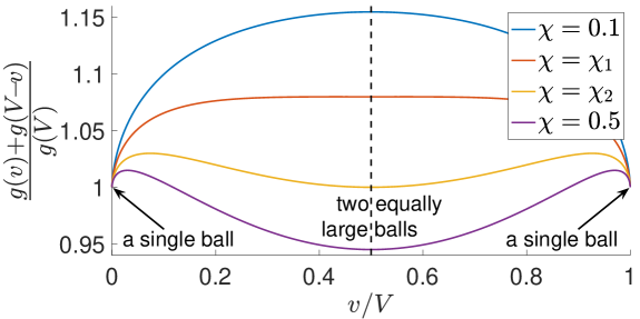
Refer to caption
Figure 21: Energy of two balls infinitely far apart. Horizontal axis: volume fraction. Vertical axis: energy ratio of two balls to one ball. Dashed vertical line: the cases where the two balls have equal radii.

The calculation of $\raisebox{2.0pt}{$\chi$}_{1}$ is straightforward by looking at the sign of the following second-order derivative:

$$\frac{\differential^{2}}{\differential v^{2}}\bigg{|}_{v=V/2}\Big{(}g(v)+g(V\!-\!v)\Big{)}=2(V\!-\!8\pi)\big{/}\sqrt[3]{81\pi^{2}V^{4}}.$$

Appendix B Euler–Lagrange equations for diffuse and sharp interfaces

In this appendix, let us formally derive (7) from (6) as $c\rightarrow 0$. Let $\Gamma$ be the interface $\big{\{}\vec{x}:\eta(\vec{x})=1/2\big{\}}$. Assuming $c\ll 1$, in the vicinity of $\Gamma$, the first two terms in the left-hand side of (6) are dominant, therefore we follow the heuristics in [21, Equation (6)] and assume that the stationary solution has the following approximation in the vicinity of $\Gamma$,

$$\eta\big{(}\vec{x}\big{)}=\frac{1+\tanh\big(kd(\vec{x})\big{missing})}{2},$$

where $k>0$ is an undetermined coefficient, and $d(\vec{x})$ is the signed distance function between $\vec{x}$ and $\Gamma$. By differentiating both sides we obtain

$\displaystyle 2\Delta\eta$ $\displaystyle=\nabla\cdot\nabla\tanh(kd)=\nabla\cdot\big{(}k\tanh^{\prime}(kd)\nabla d\big{)}$
$\displaystyle=k\,\nabla\tanh^{\prime}(kd)\cdot\nabla d+k\tanh^{\prime}(kd)\Delta d$
$\displaystyle=k^{2}\tanh^{\prime\prime}(kd)\nabla d\cdot\nabla d+k\tanh^{\prime}(kd)\Delta d,$

where

$$\tanh^{\prime}=1-\tanh^{2}=\frac{2}{3}f^{\prime}\Big{(}\frac{1\!+\!\tanh}{2}\Big{)},\quad\tanh^{\prime\prime}=2\tanh^{3}-2\tanh=\frac{4}{3}W^{\prime}\Big{(}\frac{1\!+\!\tanh}{2}\Big{)}.$$

According to [21, Bottom of Page 11], we have $\nabla d\cdot\nabla d=\|\nabla d\|_{2}^{2}=1$ and $\Delta d=-(n\!-\!1)H$. Therefore

$\displaystyle\sqrt{6/c}\,W^{\prime}(\eta)-\sqrt{6c}\,\Delta\hskip 0.5pt\eta$ $\displaystyle=\sqrt{\frac{6}{c}}\,W^{\prime}(\eta)-\sqrt{\frac{3c}{2}}\big{(}k^{2}\tanh^{\prime\prime}(kd)-(n\!-\!1)Hk\tanh^{\prime}(kd)\big{)}$
$\displaystyle=\sqrt{\frac{6}{c}}\,W^{\prime}(\eta)-\sqrt{\frac{3c}{2}}\Big{(}k^{2}\frac{4}{3}W^{\prime}(\eta)-(n\!-\!1)Hk\frac{2}{3}f^{\prime}(\eta)\Big{)}$
$\displaystyle=\Big{(}\sqrt{\frac{6}{c}}\!-\!\sqrt{\frac{8c}{3}}k^{2}\Big{)}W^{\prime}(\eta)+\sqrt{\frac{2c}{3}}(n\!-\!1)Hkf^{\prime}(\eta),$

where we choose $k=\sqrt{3/(2c)}$ so that the coefficient of $W^{\prime}(\eta)$ vanishes. In this way, in the vicinity of $\Gamma$, we can rewrite (6) as

$$(n\!-\!1)Hf^{\prime}(\eta)-\tilde{\gamma}f^{\prime}(\eta)\,\Delta^{-1}f(\eta)=-Kf^{\prime}(\eta)\big{\langle}f(\eta)\!-\!\omega,\,1\big{\rangle},$$

or equivalently

$$(n\!-\!1)H+\tilde{\gamma}(-\Delta)^{-1}f(\eta)=-K\big{\langle}f(\eta)\!-\!\omega,\,1\big{\rangle},$$

where the right-hand side can be regarded as a Lagrange multiplier, and $f(\eta)$ converges to some indicator function $\bm{1}_{\Omega}$ as $c\rightarrow 0$.

Appendix C Stability of a strip or a lamella against rupture

In this appendix, we consider the periodic isoperimetric problem [15, Equation (3.10)] in a unit cell. A thin strip (in 2-D) or a thin lamella (in 3-D) may have relatively large interfacial energy, but we are going to show that they are both stable against a certain class of perturbations.

C.1 The 2-D case

Let the periodic cell be $[0,1]^{2}$. Without loss of generality, we only consider shapes described by $\big{\{}(x,y):0<y<f(x)\big{\}}$, where $f:[0,1]\to[0,1]$ is piecewise continuously differentiable and satisfies the periodic boundary condition $f(0)=f(1)$. Given $\omega\in(0,1)$, the periodic isoperimetric problem can be written as follows

$$\min_{f}\text{Per}(f)\quad\text{subject to}\quad\text{Area}(f)=\omega,$$ (12)

where

$$\text{Per}(f)=\int_{0}^{1}\sqrt{f^{\prime}(x)^{2}\!+\!1}\differential{x}\quad\text{and}\quad\text{Area}(f)=\int_{0}^{1}f(x)\differential{x}.$$

The following proposition shows that no matter how small $\omega$ is, a thin strip is always stable against admissible deformations.

Proposition C.1.

For any $\omega\in(0,1)$, the second-order variation of (12) at the constant function $f=\omega$ is positive among admissible perturbations.

Proof. For the constant function $f=\omega$, consider the deformation from $f$ to $f+\varepsilon g$, where $0<\varepsilon\ll 1$, and $g$ is piecewise continuously differentiable and satisfies the periodic boundary condition $g(0)=g(1)$. Using Taylor expansion we obtain

$$\text{Per}(f+\varepsilon g)=\text{Per}(f)+\varepsilon\!\int_{0}^{1}\frac{f^{\prime}(x)g^{\prime}(x)}{\sqrt{f^{\prime}(x)^{2}\!+\!1}}\differential{x}+\frac{\varepsilon^{2}}{2}\!\int\frac{g^{\prime}(x)^{2}\differential{x}}{\big{(}f^{\prime}(x)^{2}\!+\!1\big{)}^{3/2}}+O\big{(}\varepsilon^{3}\big{)},$$

where the first-order term (involving $\varepsilon$) is always zero, and the second-order term (involving $\varepsilon^{2}$) is always positive unless $g=0$, because we have $f^{\prime}=0$. ∎

C.2 The 3-D case

Let the periodic cell be $[0,1]^{3}$. Without loss of generality, we only consider shapes described by $\big{\{}(x,y,z):0<z<f(x,y)\big{\}}$, where $f:[0,1]^{2}\to[0,1]$ is piecewise continuously differentiable and satisfies periodic boundary conditions. Given $\omega\in(0,1)$, the periodic isoperimetric problem can be written as follows

$$\min_{f}\text{Area}(f)\quad\text{subject to}\quad\text{Vol}(f)=\omega,$$ (13)

where

$$\text{Area}(f)=\iint_{[0,\,1]^{2}}\sqrt{f_{x}^{2}\!+\!f_{y}^{2}\!+\!1}\differential{x}\differential{y}\quad\text{and}\quad\text{Vol}(f)=\iint_{[0,\,1]^{2}}f\differential{x}\differential{y},$$

with $f_{x}$ and $f_{y}$ denoting the partial derivatives of $f$. The following proposition shows that no matter how small $\omega$ is, a thin lamella is always stable against admissible deformations.

Proposition C.2.

For any $\omega\in(0,1)$, the second-order variation of (13) at the constant function $f=\omega$ is positive among admissible perturbations.

Proof. For the constant function $f=\omega$, consider the deformation from $f$ to $f+\varepsilon g$, where $0<\varepsilon\ll 1$, and $g$ is piecewise continuously differentiable and satisfies periodic boundary conditions. Using Taylor expansion we obtain

$$\text{Area}(f+\varepsilon g)=\text{Area}(f)+\varepsilon\iint\frac{(f_{x}g_{x}\!+\!f_{y}g_{y})}{\sqrt{f_{x}^{2}\!+\!f_{y}^{2}+1}}+\frac{\varepsilon^{2}}{2}\!\iint\frac{f_{x}^{2}g_{y}^{2}\!-\!2f_{x}f_{y}g_{x}g_{y}\!+\!f_{y}^{2}g_{x}^{2}\!+\!g_{x}^{2}\!+\!g_{y}^{2}}{\left(f_{x}^{2}+f_{y}^{2}+1\right)^{3/2}}+O\big{(}\varepsilon^{3}\big{)},$$

where the first-order term (involving $\varepsilon$) is always zero, and the second-order term (involving $\varepsilon^{2}$) is always positive unless $g=0$, because we have $f_{x}=f_{y}=0$. ∎

Appendix D Algorithms for $(-\Delta)^{-1}$ under no boundary conditions

In this appendix, we provide code for numerically solving Poisson’s equation $-\Delta\phi=\eta$ in the free space.

D.1 The 2-D case

As an example, we use the source term $\eta$ given by (14).

Listing 1: MATLAB code for solving Poisson’s equation in 2-D
M = 256; N = 256; X = 1; Y = 1;
r = radius(1:N,(1:M)’,M,N,X,Y);
eta = 1 - 12*min(r,1/2).^2 + 16*min(r,1/2).^3;
phi_analytical = Poisson_Analytical(r);
phi_numerical = Poisson_Numerical(eta, X, Y);
err = max(abs(phi_analytical(:)-phi_numerical(:)));
fprintf(’For [M,N] = [%d,%d], the error is %g.\n’,M,N,err);
function r = radius(i,j,M,N,X,Y)
xi = X/N*(i-1/2); yj = Y/M*(j-1/2); % 1<=i<=N, 1<=j<=M
r = sqrt((xi-X/2).^2 + (yj-Y/2).^2); % calculate distance
end
function phi = Poisson_Analytical(r)
r1 = min(r,1/2); r2 = max(r,1/2);
phi = (3*r1.^4-r1.^2)/4 - 16*r1.^5/25 + 57/1600 - 3/80*log(r2);
end
function phi = Poisson_Numerical(eta, X, Y)
[M, N] = size(eta); x = X/N*((0:N)-1/2); y = Y/M*((0:M)-1/2)’;
H = (y.^2-x.^2).*atan(x./y) + x.*y.*log(x.^2+y.^2);
Gh = diff(diff(H),1,2) - 3*X/N*Y/M;
Gh(1,:) = Gh(1,:) + 2*pi*(X/N)^2*(0:N-1);
Gh(1,1) = Gh(1,1) + pi/2*(X/N)^2; Gh = Gh/(-4*pi);
Gh = [Gh(end:-1:2,:);Gh;zeros(1,N)];
Gh = [Gh(:,end:-1:2) Gh zeros(2*M,1)];
convolution = ifft2(fft2(eta,2*M,2*N).*fft2(Gh));
phi = real(convolution(end-M:end-1,end-N:end-1));
end
\mlttfamily

D.2 The 3-D case

Listing 2: MATLAB code for solving Poisson’s equation in 3-D
function phi = Poisson_Numerical(eta, X, Y, Z)
[M, N, P] = size(eta); x = X/N*((0:N)-1/2);
y = Y/M*((0:M)-1/2)’; z = reshape(Z/P*((0:P)-1/2),1,1,[]);
xy = x.*y; yz = y.*z; zx = z.*x; r = sqrt(x.^2+y.^2+z.^2);
H = yz.*log(x+r) + zx.*log(y+r) + xy.*log(z+r) -…
x.^2/2.*atan(yz./(x.*r)) - y.^2/2.*atan(zx./(y.*r)) -…
z.^2/2.*atan(xy./(z.*r));
Gh = diff(diff(diff(H),1,2),1,3); Gh = Gh/(4*pi);
Gh = cat(1, Gh(end:-1:2,:,:), Gh, zeros(1, N,P));
Gh = cat(2, Gh(:,end:-1:2,:), Gh, zeros(2*M, 1,P));
Gh = cat(3, Gh(:,:,end:-1:2), Gh, zeros(2*M,2*N,1));
convolution = ifftn(fftn(eta,[2*M,2*N,2*P]).*fftn(Gh));
phi = real(convolution(end-M:end-1,end-N:end-1,end-P:end-1));
end
\mlttfamily

D.3 Numerical convergence

As a test run, we compute the Poisson potential of the following source term in 2-D:

$$\eta(x,y)=\left\{\begin{aligned} &1\!-\!12r^{2}\!+\!16r^{3},&&r\leqslant\frac{1}{2},\\ &0,&&r>\frac{1}{2},\end{aligned}\right.\quad\text{where}\;r:=\sqrt{\Big{(}x\!-\!\frac{1}{2}\Big{)}^{2}+\Big{(}y\!-\!\frac{1}{2}\Big{)}^{2}}.$$ (14)

We know that $\eta$ is axisymmetric and compactly supported within $[0,1]^{2}$, as shown on the left of Figure 22. The potential $\phi$ is given by the convolution $G*\eta$, where $G(x,y)=(-4\pi)^{-1}\ln(x^{2}\!+\!y^{2})$. We know that $\phi$ is also axisymmetric, as shown on the right of Figure 22, and has an analytic expression

$$\phi(x,y)=\left\{\begin{aligned} &\frac{3r^{4}\!-\!r^{2}}{4}-\frac{16r^{5}}{25}+\frac{57}{1600}+\frac{3\ln 2}{80},&&r\leqslant\frac{1}{2},\\ &-\frac{3\ln r}{80},&&r>\frac{1}{2}.\end{aligned}\right.$$ (15)

See [10] for the derivation in the case of $r>1/2$. The case of $r\leqslant 1/2$ can be derived using polar coordinates for Laplacian, and then adding a constant term to make $\phi$ continuous.

Refer to caption
Refer to caption
Figure 22: Test run. Left: source term. Right: Poisson potential.

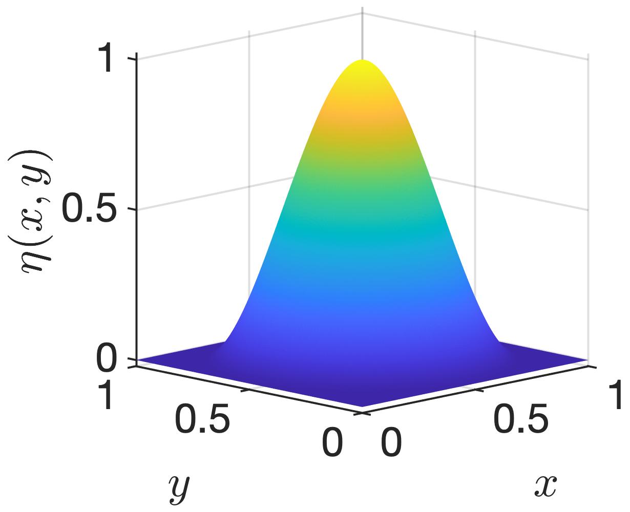
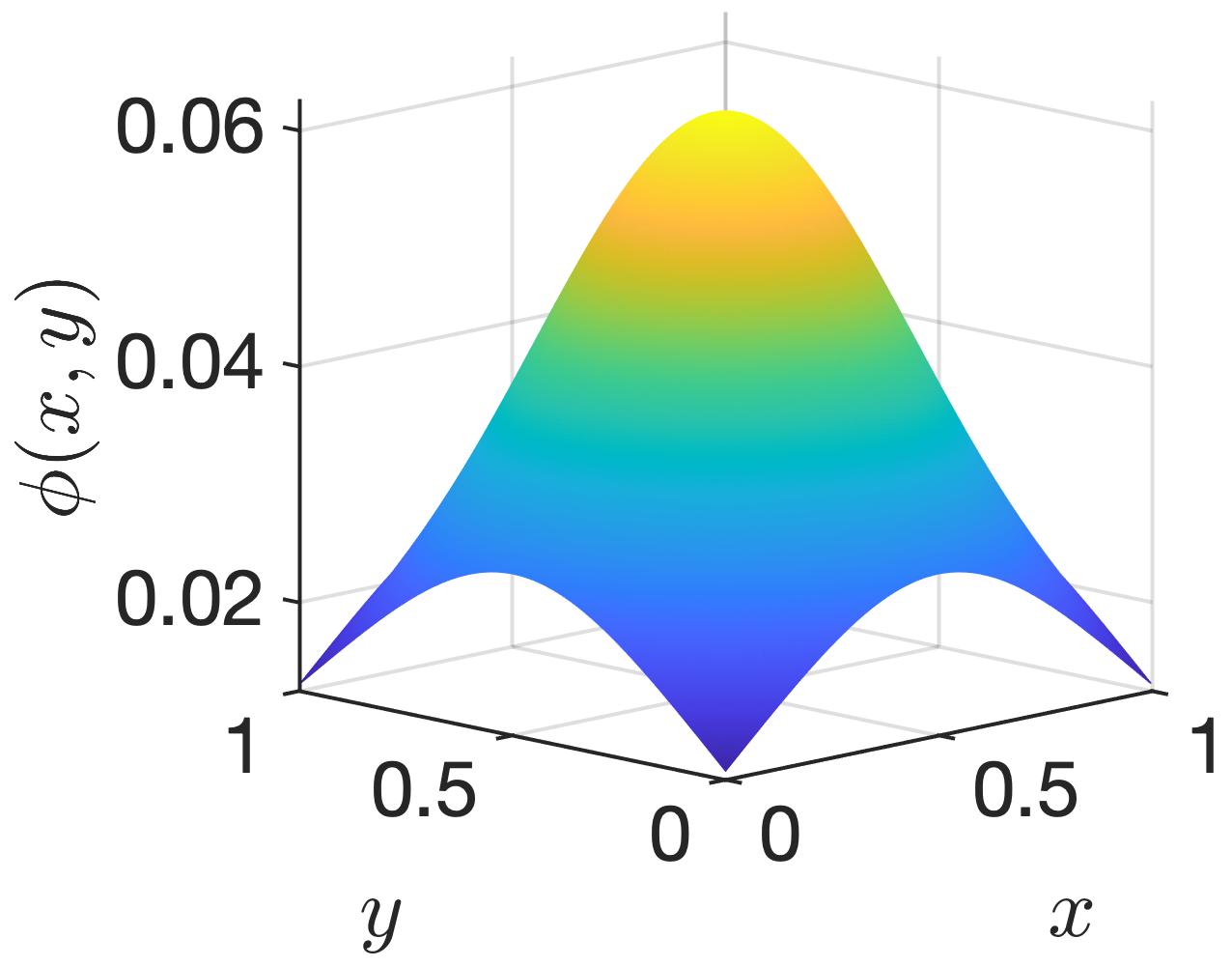
We look at the difference between the analytic solution (15) and the numerical solution obtained in Appendix D.1. Define the error to be the maximum difference on all the grid points. Our numerical results exhibit quadratic convergence, as shown in Table 1.

Table 1: Convergence
$[M,N]$ error ratio
$[64,64]$ $1.02\times 10^{-5}$ 4.00
$[128,128]$ $2.54\times 10^{-6}$ 4.00
$[256,256]$ $6.36\times 10^{-7}$ 4.00
$[512,512]$ $1.59\times 10^{-7}$

Appendix E Simulations in 3-D under no boundary conditions

In this appendix we present the detailed numerical results for the minimum energy paths of fission in 3-D under no boundary conditions.

Refer to caption

aRefer to captionRefer to captiona\overset{\includegraphics[width=58.0pt]{images/NoBoundary3D/8.0/a.png}}{\begin{minipage}[t][0pt][b]{24.0pt}\hskip 7.0pta\end{minipage}} bRefer to captionRefer to captionb\overset{\includegraphics[width=58.0pt]{images/NoBoundary3D/8.0/b.png}}{\begin{minipage}[t][0pt][b]{24.0pt}\hskip 7.0ptb\end{minipage}} cRefer to captionRefer to captionc\overset{\includegraphics[width=58.0pt]{images/NoBoundary3D/8.0/c.png}}{\begin{minipage}[t][0pt][b]{24.0pt}\hskip 7.0ptc\end{minipage}} dRefer to captionRefer to captiond\overset{\includegraphics[width=58.0pt]{images/NoBoundary3D/8.0/d.png}}{\begin{minipage}[t][0pt][b]{24.0pt}\hskip 7.0ptd\end{minipage}} eRefer to captionRefer to captione\overset{\includegraphics[width=58.0pt]{images/NoBoundary3D/8.0/e.png}}{\begin{minipage}[t][0pt][b]{24.0pt}\hskip 7.0pte\end{minipage}}

Figure 23: Minimum energy path ($\raisebox{2.0pt}{$\widetilde{\chi}$}=0.992$). Saddle point and scission point are b and d, respectively.
Refer to caption

aRefer to captionRefer to captiona\overset{\includegraphics[width=58.0pt]{images/NoBoundary3D/7.5/a.png}}{\begin{minipage}[t][0pt][b]{24.0pt}\hskip 7.0pta\end{minipage}} bRefer to captionRefer to captionb\overset{\includegraphics[width=58.0pt]{images/NoBoundary3D/7.5/b.png}}{\begin{minipage}[t][0pt][b]{24.0pt}\hskip 7.0ptb\end{minipage}} cRefer to captionRefer to captionc\overset{\includegraphics[width=58.0pt]{images/NoBoundary3D/7.5/c.png}}{\begin{minipage}[t][0pt][b]{24.0pt}\hskip 7.0ptc\end{minipage}} dRefer to captionRefer to captiond\overset{\includegraphics[width=58.0pt]{images/NoBoundary3D/7.5/d.png}}{\begin{minipage}[t][0pt][b]{24.0pt}\hskip 7.0ptd\end{minipage}} eRefer to captionRefer to captione\overset{\includegraphics[width=58.0pt]{images/NoBoundary3D/7.5/e.png}}{\begin{minipage}[t][0pt][b]{24.0pt}\hskip 7.0pte\end{minipage}}

Figure 24: Minimum energy path ($\raisebox{2.0pt}{$\widetilde{\chi}$}=0.930$). Saddle point and scission point are b and d, respectively.
Refer to caption

aRefer to captionRefer to captiona\overset{\includegraphics[width=58.0pt]{images/NoBoundary3D/6.8/a.png}}{\begin{minipage}[t][0pt][b]{24.0pt}\hskip 7.0pta\end{minipage}} bRefer to captionRefer to captionb\overset{\includegraphics[width=58.0pt]{images/NoBoundary3D/6.8/b.png}}{\begin{minipage}[t][0pt][b]{24.0pt}\hskip 7.0ptb\end{minipage}} cRefer to captionRefer to captionc\overset{\includegraphics[width=58.0pt]{images/NoBoundary3D/6.8/c.png}}{\begin{minipage}[t][0pt][b]{24.0pt}\hskip 7.0ptc\end{minipage}} dRefer to captionRefer to captiond\overset{\includegraphics[width=58.0pt]{images/NoBoundary3D/6.8/d.png}}{\begin{minipage}[t][0pt][b]{24.0pt}\hskip 7.0ptd\end{minipage}} eRefer to captionRefer to captione\overset{\includegraphics[width=58.0pt]{images/NoBoundary3D/6.8/e.png}}{\begin{minipage}[t][0pt][b]{24.0pt}\hskip 7.0pte\end{minipage}}

Figure 25: Minimum energy path ($\raisebox{2.0pt}{$\widetilde{\chi}$}=0.844$). Saddle point and scission point are b and d, respectively.
Refer to caption

aRefer to captionRefer to captiona\overset{\includegraphics[width=58.0pt]{images/NoBoundary3D/6.0/a.png}}{\begin{minipage}[t][0pt][b]{24.0pt}\hskip 7.0pta\end{minipage}} bRefer to captionRefer to captionb\overset{\includegraphics[width=58.0pt]{images/NoBoundary3D/6.0/b.png}}{\begin{minipage}[t][0pt][b]{24.0pt}\hskip 7.0ptb\end{minipage}} cRefer to captionRefer to captionc\overset{\includegraphics[width=58.0pt]{images/NoBoundary3D/6.0/c.png}}{\begin{minipage}[t][0pt][b]{24.0pt}\hskip 7.0ptc\end{minipage}} dRefer to captionRefer to captiond\overset{\includegraphics[width=58.0pt]{images/NoBoundary3D/6.0/d.png}}{\begin{minipage}[t][0pt][b]{24.0pt}\hskip 7.0ptd\end{minipage}} eRefer to captionRefer to captione\overset{\includegraphics[width=58.0pt]{images/NoBoundary3D/6.0/e.png}}{\begin{minipage}[t][0pt][b]{24.0pt}\hskip 7.0pte\end{minipage}}

Figure 26: Minimum energy path ($\raisebox{2.0pt}{$\widetilde{\chi}$}=0.744$). Saddle point and scission point are c and d, respectively.
Refer to caption

aRefer to captionRefer to captiona\overset{\includegraphics[width=58.0pt]{images/NoBoundary3D/5.3/a.png}}{\begin{minipage}[t][0pt][b]{24.0pt}\hskip 7.0pta\end{minipage}} bRefer to captionRefer to captionb\overset{\includegraphics[width=58.0pt]{images/NoBoundary3D/5.3/b.png}}{\begin{minipage}[t][0pt][b]{24.0pt}\hskip 7.0ptb\end{minipage}} cRefer to captionRefer to captionc\overset{\includegraphics[width=58.0pt]{images/NoBoundary3D/5.3/c.png}}{\begin{minipage}[t][0pt][b]{24.0pt}\hskip 7.0ptc\end{minipage}} dRefer to captionRefer to captiond\overset{\includegraphics[width=58.0pt]{images/NoBoundary3D/5.3/d.png}}{\begin{minipage}[t][0pt][b]{24.0pt}\hskip 7.0ptd\end{minipage}} eRefer to captionRefer to captione\overset{\includegraphics[width=58.0pt]{images/NoBoundary3D/5.3/e.png}}{\begin{minipage}[t][0pt][b]{24.0pt}\hskip 7.0pte\end{minipage}}

Figure 27: Minimum energy path ($\raisebox{2.0pt}{$\widetilde{\chi}$}=0.657$). Saddle point and scission point are c and d, respectively.
Refer to caption

aRefer to captionRefer to captiona\overset{\includegraphics[width=58.0pt]{images/NoBoundary3D/4.7/a.png}}{\begin{minipage}[t][0pt][b]{24.0pt}\hskip 7.0pta\end{minipage}} bRefer to captionRefer to captionb\overset{\includegraphics[width=58.0pt]{images/NoBoundary3D/4.7/b.png}}{\begin{minipage}[t][0pt][b]{24.0pt}\hskip 7.0ptb\end{minipage}} cRefer to captionRefer to captionc\overset{\includegraphics[width=58.0pt]{images/NoBoundary3D/4.7/c.png}}{\begin{minipage}[t][0pt][b]{24.0pt}\hskip 7.0ptc\end{minipage}} dRefer to captionRefer to captiond\overset{\includegraphics[width=58.0pt]{images/NoBoundary3D/4.7/d.png}}{\begin{minipage}[t][0pt][b]{24.0pt}\hskip 7.0ptd\end{minipage}} eRefer to captionRefer to captione\overset{\includegraphics[width=58.0pt]{images/NoBoundary3D/4.7/e.png}}{\begin{minipage}[t][0pt][b]{24.0pt}\hskip 7.0pte\end{minipage}}

Figure 28: Minimum energy path ($\raisebox{2.0pt}{$\widetilde{\chi}$}=0.583$). Saddle point and scission point are c and d, respectively.
Refer to caption

aRefer to captionRefer to captiona\overset{\includegraphics[width=58.0pt]{images/NoBoundary3D/3.2/a.png}}{\begin{minipage}[t][0pt][b]{24.0pt}\hskip 7.0pta\end{minipage}} bRefer to captionRefer to captionb\overset{\includegraphics[width=58.0pt]{images/NoBoundary3D/3.2/b.png}}{\begin{minipage}[t][0pt][b]{24.0pt}\hskip 7.0ptb\end{minipage}} cRefer to captionRefer to captionc\overset{\includegraphics[width=58.0pt]{images/NoBoundary3D/3.2/c.png}}{\begin{minipage}[t][0pt][b]{24.0pt}\hskip 7.0ptc\end{minipage}} dRefer to captionRefer to captiond\overset{\includegraphics[width=58.0pt]{images/NoBoundary3D/3.2/d.png}}{\begin{minipage}[t][0pt][b]{24.0pt}\hskip 7.0ptd\end{minipage}} eRefer to captionRefer to captione\overset{\includegraphics[width=58.0pt]{images/NoBoundary3D/3.2/e.png}}{\begin{minipage}[t][0pt][b]{24.0pt}\hskip 7.0pte\end{minipage}}

Figure 29: Minimum energy path ($\raisebox{2.0pt}{$\widetilde{\chi}$}=0.397$). Saddle point and scission point are c and d, respectively.

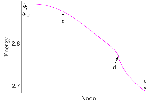
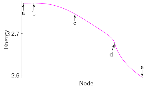
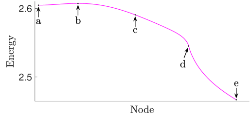
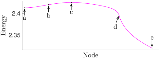
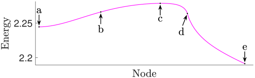
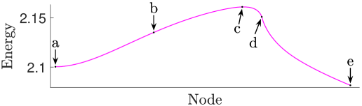
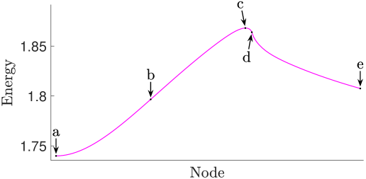
Appendix F Simulations in 3-D under periodic boundary conditions

In this appendix we present the numerical simulations of (2) in 3-D under periodic boundary conditions. As mentioned in (3), the parameter $\widetilde{\chi}$ refers to $\tilde{\gamma}\omega|D|/(40\pi)$, where we choose $\omega|D|=0.04$. The results here are similar to those under no boundary conditions (in Section 4), and we expect the former to converge to the latter as $\omega\rightarrow 0$.

We numerically study the pACOK dynamics with the initial value resembling the indicator function of a ball. According to our simulation results, there is a critical value $\raisebox{2.0pt}{$\widetilde{\chi}$}_{*}\in(1.086,1.092)$ such that for $\raisebox{2.0pt}{$\widetilde{\chi}$}<\raisebox{2.0pt}{$\widetilde{\chi}$}_{*}$, the ball is stable; for $\raisebox{2.0pt}{$\widetilde{\chi}$}>\raisebox{2.0pt}{$\widetilde{\chi}$}_{*}$, the ball is unstable and will eventually split into two equally large balls. Due to periodic boundary conditions, those two balls will align themselves along a body diagonal of the simulation box and keep distance from the boundaries.

We use the string method to compute the minimum energy paths. The is a critical value $\raisebox{2.0pt}{$\widetilde{\chi}$}_{3}\in(0.463,0.469)$ such that for $\raisebox{2.0pt}{$\widetilde{\chi}$}<\raisebox{2.0pt}{$\widetilde{\chi}$}_{3}$, the computed minimum energy path of fission is unstable against mass-asymmetric perturbations. After sufficiently many iterations in the string method, such a fission path will eventually converge to another minimum energy path, which we call the spallation path (named after the spallation process described in [16, Page 144]). Along the spallation path, a tiny child ball emerges at a distance from the parent ball, and then the child ball grows while the parent ball shrinks, until they achieve equal sizes. This spallation path can be understood as the reverse process of Ostwald ripening phenomenon (or coarsening effect) [51]. For $\raisebox{2.0pt}{$\widetilde{\chi}$}>\raisebox{2.0pt}{$\widetilde{\chi}$}_{3}$, we obtain two possible minimum energy paths: fission and spallation.

Refer to caption

aRefer to captionRefer to captiona\overset{\includegraphics[width=58.0pt]{images/Periodic3D/gamma=19/a.png}}{\begin{minipage}[t][0pt][b]{24.0pt}\hskip 7.0pta\end{minipage}} bRefer to captionRefer to captionb\overset{\includegraphics[width=58.0pt]{images/Periodic3D/gamma=19/b.png}}{\begin{minipage}[t][0pt][b]{24.0pt}\hskip 7.0ptb\end{minipage}} cRefer to captionRefer to captionc\overset{\includegraphics[width=58.0pt]{images/Periodic3D/gamma=19/c.png}}{\begin{minipage}[t][0pt][b]{24.0pt}\hskip 7.0ptc\end{minipage}} dRefer to captionRefer to captiond\overset{\includegraphics[width=58.0pt]{images/Periodic3D/gamma=19/d.png}}{\begin{minipage}[t][0pt][b]{24.0pt}\hskip 7.0ptd\end{minipage}}

eRefer to captionRefer to captione\overset{\includegraphics[width=58.0pt]{images/Periodic3D/gamma=19/e.png}}{\begin{minipage}[t][0pt][b]{24.0pt}\hskip 7.0pte\end{minipage}} fRefer to captionRefer to captionf\overset{\includegraphics[width=58.0pt]{images/Periodic3D/gamma=19/f.png}}{\begin{minipage}[t][0pt][b]{24.0pt}\hskip 7.0ptf\end{minipage}} gRefer to captionRefer to captiong\overset{\includegraphics[width=58.0pt]{images/Periodic3D/gamma=19/g.png}}{\begin{minipage}[t][0pt][b]{24.0pt}\hskip 7.0ptg\end{minipage}} hRefer to captionRefer to captionh\overset{\includegraphics[width=58.0pt]{images/Periodic3D/gamma=19/h.png}}{\begin{minipage}[t][0pt][b]{24.0pt}\hskip 7.0pth\end{minipage}}

Figure 30: Minimum energy paths ($\raisebox{2.0pt}{$\widetilde{\chi}$}=1.048$). Saddle points are b and f. Scission point is d.
Refer to caption

aRefer to captionRefer to captiona\overset{\includegraphics[width=58.0pt]{images/Periodic3D/gamma=16/a.png}}{\begin{minipage}[t][0pt][b]{24.0pt}\hskip 7.0pta\end{minipage}} bRefer to captionRefer to captionb\overset{\includegraphics[width=58.0pt]{images/Periodic3D/gamma=16/b.png}}{\begin{minipage}[t][0pt][b]{24.0pt}\hskip 7.0ptb\end{minipage}} cRefer to captionRefer to captionc\overset{\includegraphics[width=58.0pt]{images/Periodic3D/gamma=16/c.png}}{\begin{minipage}[t][0pt][b]{24.0pt}\hskip 7.0ptc\end{minipage}} dRefer to captionRefer to captiond\overset{\includegraphics[width=58.0pt]{images/Periodic3D/gamma=16/d.png}}{\begin{minipage}[t][0pt][b]{24.0pt}\hskip 7.0ptd\end{minipage}}

eRefer to captionRefer to captione\overset{\includegraphics[width=58.0pt]{images/Periodic3D/gamma=16/e.png}}{\begin{minipage}[t][0pt][b]{24.0pt}\hskip 7.0pte\end{minipage}} fRefer to captionRefer to captionf\overset{\includegraphics[width=58.0pt]{images/Periodic3D/gamma=16/f.png}}{\begin{minipage}[t][0pt][b]{24.0pt}\hskip 7.0ptf\end{minipage}} gRefer to captionRefer to captiong\overset{\includegraphics[width=58.0pt]{images/Periodic3D/gamma=16/g.png}}{\begin{minipage}[t][0pt][b]{24.0pt}\hskip 7.0ptg\end{minipage}} hRefer to captionRefer to captionh\overset{\includegraphics[width=58.0pt]{images/Periodic3D/gamma=16/h.png}}{\begin{minipage}[t][0pt][b]{24.0pt}\hskip 7.0pth\end{minipage}}

Figure 31: Minimum energy paths ($\raisebox{2.0pt}{$\widetilde{\chi}$}=0.882$). Saddle points are b and f. Scission point is d.
Refer to caption

aRefer to captionRefer to captiona\overset{\includegraphics[width=58.0pt]{images/Periodic3D/gamma=15/a.png}}{\begin{minipage}[t][0pt][b]{24.0pt}\hskip 7.0pta\end{minipage}} bRefer to captionRefer to captionb\overset{\includegraphics[width=58.0pt]{images/Periodic3D/gamma=15/b.png}}{\begin{minipage}[t][0pt][b]{24.0pt}\hskip 7.0ptb\end{minipage}} cRefer to captionRefer to captionc\overset{\includegraphics[width=58.0pt]{images/Periodic3D/gamma=15/c.png}}{\begin{minipage}[t][0pt][b]{24.0pt}\hskip 7.0ptc\end{minipage}} dRefer to captionRefer to captiond\overset{\includegraphics[width=58.0pt]{images/Periodic3D/gamma=15/d.png}}{\begin{minipage}[t][0pt][b]{24.0pt}\hskip 7.0ptd\end{minipage}}

eRefer to captionRefer to captione\overset{\includegraphics[width=58.0pt]{images/Periodic3D/gamma=15/e.png}}{\begin{minipage}[t][0pt][b]{24.0pt}\hskip 7.0pte\end{minipage}} fRefer to captionRefer to captionf\overset{\includegraphics[width=58.0pt]{images/Periodic3D/gamma=15/f.png}}{\begin{minipage}[t][0pt][b]{24.0pt}\hskip 7.0ptf\end{minipage}} gRefer to captionRefer to captiong\overset{\includegraphics[width=58.0pt]{images/Periodic3D/gamma=15/g.png}}{\begin{minipage}[t][0pt][b]{24.0pt}\hskip 7.0ptg\end{minipage}} hRefer to captionRefer to captionh\overset{\includegraphics[width=58.0pt]{images/Periodic3D/gamma=15/h.png}}{\begin{minipage}[t][0pt][b]{24.0pt}\hskip 7.0pth\end{minipage}}

Figure 32: Minimum energy paths ($\raisebox{2.0pt}{$\widetilde{\chi}$}=0.827$). Saddle points are c and f. Scission point is d.
Refer to caption

aRefer to captionRefer to captiona\overset{\includegraphics[width=58.0pt]{images/Periodic3D/gamma=13.5/a.png}}{\begin{minipage}[t][0pt][b]{24.0pt}\hskip 7.0pta\end{minipage}} bRefer to captionRefer to captionb\overset{\includegraphics[width=58.0pt]{images/Periodic3D/gamma=13.5/b.png}}{\begin{minipage}[t][0pt][b]{24.0pt}\hskip 7.0ptb\end{minipage}} cRefer to captionRefer to captionc\overset{\includegraphics[width=58.0pt]{images/Periodic3D/gamma=13.5/c.png}}{\begin{minipage}[t][0pt][b]{24.0pt}\hskip 7.0ptc\end{minipage}} dRefer to captionRefer to captiond\overset{\includegraphics[width=58.0pt]{images/Periodic3D/gamma=13.5/d.png}}{\begin{minipage}[t][0pt][b]{24.0pt}\hskip 7.0ptd\end{minipage}}

eRefer to captionRefer to captione\overset{\includegraphics[width=58.0pt]{images/Periodic3D/gamma=13.5/e.png}}{\begin{minipage}[t][0pt][b]{24.0pt}\hskip 7.0pte\end{minipage}} fRefer to captionRefer to captionf\overset{\includegraphics[width=58.0pt]{images/Periodic3D/gamma=13.5/f.png}}{\begin{minipage}[t][0pt][b]{24.0pt}\hskip 7.0ptf\end{minipage}} gRefer to captionRefer to captiong\overset{\includegraphics[width=58.0pt]{images/Periodic3D/gamma=13.5/g.png}}{\begin{minipage}[t][0pt][b]{24.0pt}\hskip 7.0ptg\end{minipage}} hRefer to captionRefer to captionh\overset{\includegraphics[width=58.0pt]{images/Periodic3D/gamma=13.5/h.png}}{\begin{minipage}[t][0pt][b]{24.0pt}\hskip 7.0pth\end{minipage}}

Figure 33: Minimum energy paths ($\raisebox{2.0pt}{$\widetilde{\chi}$}=0.744$). Saddle points are c and f. Scission point is d.
Refer to caption

aRefer to captionRefer to captiona\overset{\includegraphics[width=58.0pt]{images/Periodic3D/gamma=8.5/a.png}}{\begin{minipage}[t][0pt][b]{24.0pt}\hskip 7.0pta\end{minipage}} bRefer to captionRefer to captionb\overset{\includegraphics[width=58.0pt]{images/Periodic3D/gamma=8.5/b.png}}{\begin{minipage}[t][0pt][b]{24.0pt}\hskip 7.0ptb\end{minipage}} cRefer to captionRefer to captionc\overset{\includegraphics[width=58.0pt]{images/Periodic3D/gamma=8.5/c.png}}{\begin{minipage}[t][0pt][b]{24.0pt}\hskip 7.0ptc\end{minipage}} dRefer to captionRefer to captiond\overset{\includegraphics[width=58.0pt]{images/Periodic3D/gamma=8.5/d.png}}{\begin{minipage}[t][0pt][b]{24.0pt}\hskip 7.0ptd\end{minipage}}

eRefer to captionRefer to captione\overset{\includegraphics[width=58.0pt]{images/Periodic3D/gamma=8.5/e.png}}{\begin{minipage}[t][0pt][b]{24.0pt}\hskip 7.0pte\end{minipage}} fRefer to captionRefer to captionf\overset{\includegraphics[width=58.0pt]{images/Periodic3D/gamma=8.5/f.png}}{\begin{minipage}[t][0pt][b]{24.0pt}\hskip 7.0ptf\end{minipage}} gRefer to captionRefer to captiong\overset{\includegraphics[width=58.0pt]{images/Periodic3D/gamma=8.5/g.png}}{\begin{minipage}[t][0pt][b]{24.0pt}\hskip 7.0ptg\end{minipage}} hRefer to captionRefer to captionh\overset{\includegraphics[width=58.0pt]{images/Periodic3D/gamma=8.5/h.png}}{\begin{minipage}[t][0pt][b]{24.0pt}\hskip 7.0pth\end{minipage}}

Figure 34: Minimum energy paths ($\raisebox{2.0pt}{$\widetilde{\chi}$}=0.469$). Saddle points are c and f. Scission point is d.

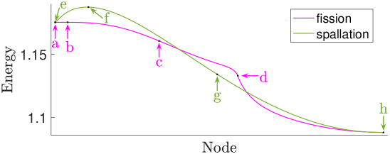
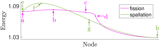
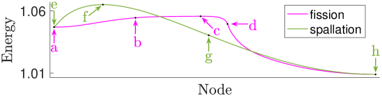
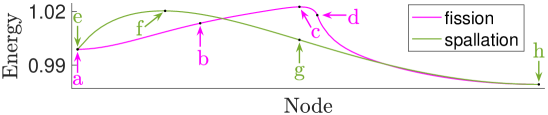
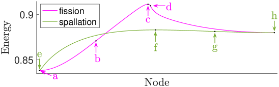
Appendix G Simulations in 2-D under no boundary conditions

In this appendix we present the detailed numerical results for the minimum energy paths of fission in 2-D under no boundary conditions.

Refer to caption

aRefer to captionRefer to captiona\overset{\includegraphics[width=53.0pt]{images/NoBoundary2D/4.69/a.png}}{\begin{minipage}[t][0pt][b]{24.0pt}\hskip 10.0pta\end{minipage}} bRefer to captionRefer to captionb\overset{\includegraphics[width=53.0pt]{images/NoBoundary2D/4.69/b.png}}{\begin{minipage}[t][0pt][b]{24.0pt}\hskip 10.0ptb\end{minipage}} cRefer to captionRefer to captionc\overset{\includegraphics[width=53.0pt]{images/NoBoundary2D/4.69/c.png}}{\begin{minipage}[t][0pt][b]{24.0pt}\hskip 10.0ptc\end{minipage}} dRefer to captionRefer to captiond\overset{\includegraphics[width=53.0pt]{images/NoBoundary2D/4.69/d.png}}{\begin{minipage}[t][0pt][b]{24.0pt}\hskip 10.0ptd\end{minipage}} eRefer to captionRefer to captione\overset{\includegraphics[width=53.0pt]{images/NoBoundary2D/4.69/e.png}}{\begin{minipage}[t][0pt][b]{24.0pt}\hskip 10.0pte\end{minipage}} fRefer to captionRefer to captionf\overset{\includegraphics[width=53.0pt]{images/NoBoundary2D/4.69/f.png}}{\begin{minipage}[t][0pt][b]{24.0pt}\hskip 10.0ptf\end{minipage}}

Figure 35: Minimum energy path ($\raisebox{2.0pt}{$\widetilde{\chi}$}\!=\!0.999$). Local minimizers are a and c. Transition states are b and d.
Refer to caption

aRefer to captionRefer to captiona\overset{\includegraphics[width=53.0pt]{images/NoBoundary2D/4.58/a.png}}{\begin{minipage}[t][0pt][b]{24.0pt}\hskip 10.0pta\end{minipage}} bRefer to captionRefer to captionb\overset{\includegraphics[width=53.0pt]{images/NoBoundary2D/4.58/b.png}}{\begin{minipage}[t][0pt][b]{24.0pt}\hskip 10.0ptb\end{minipage}} cRefer to captionRefer to captionc\overset{\includegraphics[width=53.0pt]{images/NoBoundary2D/4.58/c.png}}{\begin{minipage}[t][0pt][b]{24.0pt}\hskip 10.0ptc\end{minipage}} dRefer to captionRefer to captiond\overset{\includegraphics[width=53.0pt]{images/NoBoundary2D/4.58/d.png}}{\begin{minipage}[t][0pt][b]{24.0pt}\hskip 10.0ptd\end{minipage}} eRefer to captionRefer to captione\overset{\includegraphics[width=53.0pt]{images/NoBoundary2D/4.58/e.png}}{\begin{minipage}[t][0pt][b]{24.0pt}\hskip 10.0pte\end{minipage}} fRefer to captionRefer to captionf\overset{\includegraphics[width=53.0pt]{images/NoBoundary2D/4.58/f.png}}{\begin{minipage}[t][0pt][b]{24.0pt}\hskip 10.0ptf\end{minipage}}

Figure 36: Minimum energy path ($\raisebox{2.0pt}{$\widetilde{\chi}$}\!=\!0.975$). Local minimizers are a and c. Transition states are b and d.
Refer to caption

aRefer to captionRefer to captiona\overset{\includegraphics[width=53.0pt]{images/NoBoundary2D/4.47/a.png}}{\begin{minipage}[t][0pt][b]{24.0pt}\hskip 10.0pta\end{minipage}} bRefer to captionRefer to captionb\overset{\includegraphics[width=53.0pt]{images/NoBoundary2D/4.47/b.png}}{\begin{minipage}[t][0pt][b]{24.0pt}\hskip 10.0ptb\end{minipage}} cRefer to captionRefer to captionc\overset{\includegraphics[width=53.0pt]{images/NoBoundary2D/4.47/c.png}}{\begin{minipage}[t][0pt][b]{24.0pt}\hskip 10.0ptc\end{minipage}} dRefer to captionRefer to captiond\overset{\includegraphics[width=53.0pt]{images/NoBoundary2D/4.47/d.png}}{\begin{minipage}[t][0pt][b]{24.0pt}\hskip 10.0ptd\end{minipage}} eRefer to captionRefer to captione\overset{\includegraphics[width=53.0pt]{images/NoBoundary2D/4.47/e.png}}{\begin{minipage}[t][0pt][b]{24.0pt}\hskip 10.0pte\end{minipage}} fRefer to captionRefer to captionf\overset{\includegraphics[width=53.0pt]{images/NoBoundary2D/4.47/f.png}}{\begin{minipage}[t][0pt][b]{24.0pt}\hskip 10.0ptf\end{minipage}}

Figure 37: Minimum energy path ($\raisebox{2.0pt}{$\widetilde{\chi}$}\!=\!0.952$). Local minimizers are a and c. Transition states are b and d.
Refer to caption

aRefer to captionRefer to captiona\overset{\includegraphics[width=53.0pt]{images/NoBoundary2D/4.36/a.png}}{\begin{minipage}[t][0pt][b]{24.0pt}\hskip 10.0pta\end{minipage}} bRefer to captionRefer to captionb\overset{\includegraphics[width=53.0pt]{images/NoBoundary2D/4.36/b.png}}{\begin{minipage}[t][0pt][b]{24.0pt}\hskip 10.0ptb\end{minipage}} cRefer to captionRefer to captionc\overset{\includegraphics[width=53.0pt]{images/NoBoundary2D/4.36/c.png}}{\begin{minipage}[t][0pt][b]{24.0pt}\hskip 10.0ptc\end{minipage}} dRefer to captionRefer to captiond\overset{\includegraphics[width=53.0pt]{images/NoBoundary2D/4.36/d.png}}{\begin{minipage}[t][0pt][b]{24.0pt}\hskip 10.0ptd\end{minipage}} eRefer to captionRefer to captione\overset{\includegraphics[width=53.0pt]{images/NoBoundary2D/4.36/e.png}}{\begin{minipage}[t][0pt][b]{24.0pt}\hskip 10.0pte\end{minipage}} fRefer to captionRefer to captionf\overset{\includegraphics[width=53.0pt]{images/NoBoundary2D/4.36/f.png}}{\begin{minipage}[t][0pt][b]{24.0pt}\hskip 10.0ptf\end{minipage}}

Figure 38: Minimum energy path ($\raisebox{2.0pt}{$\widetilde{\chi}$}\!=\!0.929$). Local minimizers are a and c. Transition states are b and d.
Refer to caption

aRefer to captionRefer to captiona\overset{\includegraphics[width=53.0pt]{images/NoBoundary2D/4.30/a.png}}{\begin{minipage}[t][0pt][b]{24.0pt}\hskip 10.0pta\end{minipage}} bRefer to captionRefer to captionb\overset{\includegraphics[width=53.0pt]{images/NoBoundary2D/4.30/b.png}}{\begin{minipage}[t][0pt][b]{24.0pt}\hskip 10.0ptb\end{minipage}} cRefer to captionRefer to captionc\overset{\includegraphics[width=53.0pt]{images/NoBoundary2D/4.30/c.png}}{\begin{minipage}[t][0pt][b]{24.0pt}\hskip 10.0ptc\end{minipage}} dRefer to captionRefer to captiond\overset{\includegraphics[width=53.0pt]{images/NoBoundary2D/4.30/d.png}}{\begin{minipage}[t][0pt][b]{24.0pt}\hskip 10.0ptd\end{minipage}} eRefer to captionRefer to captione\overset{\includegraphics[width=53.0pt]{images/NoBoundary2D/4.30/e.png}}{\begin{minipage}[t][0pt][b]{24.0pt}\hskip 10.0pte\end{minipage}} fRefer to captionRefer to captionf\overset{\includegraphics[width=53.0pt]{images/NoBoundary2D/4.30/f.png}}{\begin{minipage}[t][0pt][b]{24.0pt}\hskip 10.0ptf\end{minipage}}

Figure 39: Minimum energy path ($\raisebox{2.0pt}{$\widetilde{\chi}$}\!=\!0.916$). Local minimizers are a and c. Transition states are b and d.
Refer to caption

aRefer to captionRefer to captiona\overset{\includegraphics[width=53.0pt]{images/NoBoundary2D/4.25/a.png}}{\begin{minipage}[t][0pt][b]{24.0pt}\hskip 10.0pta\end{minipage}} bRefer to captionRefer to captionb\overset{\includegraphics[width=53.0pt]{images/NoBoundary2D/4.25/b.png}}{\begin{minipage}[t][0pt][b]{24.0pt}\hskip 10.0ptb\end{minipage}} cRefer to captionRefer to captionc\overset{\includegraphics[width=53.0pt]{images/NoBoundary2D/4.25/c.png}}{\begin{minipage}[t][0pt][b]{24.0pt}\hskip 10.0ptc\end{minipage}} dRefer to captionRefer to captiond\overset{\includegraphics[width=53.0pt]{images/NoBoundary2D/4.25/d.png}}{\begin{minipage}[t][0pt][b]{24.0pt}\hskip 10.0ptd\end{minipage}} eRefer to captionRefer to captione\overset{\includegraphics[width=53.0pt]{images/NoBoundary2D/4.25/e.png}}{\begin{minipage}[t][0pt][b]{24.0pt}\hskip 10.0pte\end{minipage}} fRefer to captionRefer to captionf\overset{\includegraphics[width=53.0pt]{images/NoBoundary2D/4.25/f.png}}{\begin{minipage}[t][0pt][b]{24.0pt}\hskip 10.0ptf\end{minipage}}

Figure 40: Minimum energy path ($\raisebox{2.0pt}{$\widetilde{\chi}$}\!=\!0.905$). Local minimizers are a and c. Transition states are b and d.
Refer to caption

aRefer to captionRefer to captiona\overset{\includegraphics[width=53.0pt]{images/NoBoundary2D/4.24/a.png}}{\begin{minipage}[t][0pt][b]{24.0pt}\hskip 10.0pta\end{minipage}} bRefer to captionRefer to captionb\overset{\includegraphics[width=53.0pt]{images/NoBoundary2D/4.24/b.png}}{\begin{minipage}[t][0pt][b]{24.0pt}\hskip 10.0ptb\end{minipage}} cRefer to captionRefer to captionc\overset{\includegraphics[width=53.0pt]{images/NoBoundary2D/4.24/c.png}}{\begin{minipage}[t][0pt][b]{24.0pt}\hskip 10.0ptc\end{minipage}} dRefer to captionRefer to captiond\overset{\includegraphics[width=53.0pt]{images/NoBoundary2D/4.24/d.png}}{\begin{minipage}[t][0pt][b]{24.0pt}\hskip 10.0ptd\end{minipage}} eRefer to captionRefer to captione\overset{\includegraphics[width=53.0pt]{images/NoBoundary2D/4.24/e.png}}{\begin{minipage}[t][0pt][b]{24.0pt}\hskip 10.0pte\end{minipage}} fRefer to captionRefer to captionf\overset{\includegraphics[width=53.0pt]{images/NoBoundary2D/4.24/f.png}}{\begin{minipage}[t][0pt][b]{24.0pt}\hskip 10.0ptf\end{minipage}}

Figure 41: Minimum energy path ($\raisebox{2.0pt}{$\widetilde{\chi}$}\!=\!0.903$). Transition state is d.
Refer to caption

aRefer to captionRefer to captiona\overset{\includegraphics[width=53.0pt]{images/NoBoundary2D/3.50/a.png}}{\begin{minipage}[t][0pt][b]{24.0pt}\hskip 10.0pta\end{minipage}} bRefer to captionRefer to captionb\overset{\includegraphics[width=53.0pt]{images/NoBoundary2D/3.50/b.png}}{\begin{minipage}[t][0pt][b]{24.0pt}\hskip 10.0ptb\end{minipage}} cRefer to captionRefer to captionc\overset{\includegraphics[width=53.0pt]{images/NoBoundary2D/3.50/c.png}}{\begin{minipage}[t][0pt][b]{24.0pt}\hskip 10.0ptc\end{minipage}} dRefer to captionRefer to captiond\overset{\includegraphics[width=53.0pt]{images/NoBoundary2D/3.50/d.png}}{\begin{minipage}[t][0pt][b]{24.0pt}\hskip 10.0ptd\end{minipage}} eRefer to captionRefer to captione\overset{\includegraphics[width=53.0pt]{images/NoBoundary2D/3.50/e.png}}{\begin{minipage}[t][0pt][b]{24.0pt}\hskip 10.0pte\end{minipage}} fRefer to captionRefer to captionf\overset{\includegraphics[width=53.0pt]{images/NoBoundary2D/3.50/f.png}}{\begin{minipage}[t][0pt][b]{24.0pt}\hskip 10.0ptf\end{minipage}}

Figure 42: Minimum energy path ($\raisebox{2.0pt}{$\widetilde{\chi}$}\!=\!0.745$). Transition state is d.
Refer to caption

aRefer to captionRefer to captiona\overset{\includegraphics[width=53.0pt]{images/NoBoundary2D/2.50/a.png}}{\begin{minipage}[t][0pt][b]{24.0pt}\hskip 10.0pta\end{minipage}} bRefer to captionRefer to captionb\overset{\includegraphics[width=53.0pt]{images/NoBoundary2D/2.50/b.png}}{\begin{minipage}[t][0pt][b]{24.0pt}\hskip 10.0ptb\end{minipage}} cRefer to captionRefer to captionc\overset{\includegraphics[width=53.0pt]{images/NoBoundary2D/2.50/c.png}}{\begin{minipage}[t][0pt][b]{24.0pt}\hskip 10.0ptc\end{minipage}} dRefer to captionRefer to captiond\overset{\includegraphics[width=53.0pt]{images/NoBoundary2D/2.50/d.png}}{\begin{minipage}[t][0pt][b]{24.0pt}\hskip 10.0ptd\end{minipage}} eRefer to captionRefer to captione\overset{\includegraphics[width=53.0pt]{images/NoBoundary2D/2.50/e.png}}{\begin{minipage}[t][0pt][b]{24.0pt}\hskip 10.0pte\end{minipage}} fRefer to captionRefer to captionf\overset{\includegraphics[width=53.0pt]{images/NoBoundary2D/2.50/f.png}}{\begin{minipage}[t][0pt][b]{24.0pt}\hskip 10.0ptf\end{minipage}}

Figure 43: Minimum energy path ($\raisebox{2.0pt}{$\widetilde{\chi}$}\!=\!0.532$). Transition state is d.

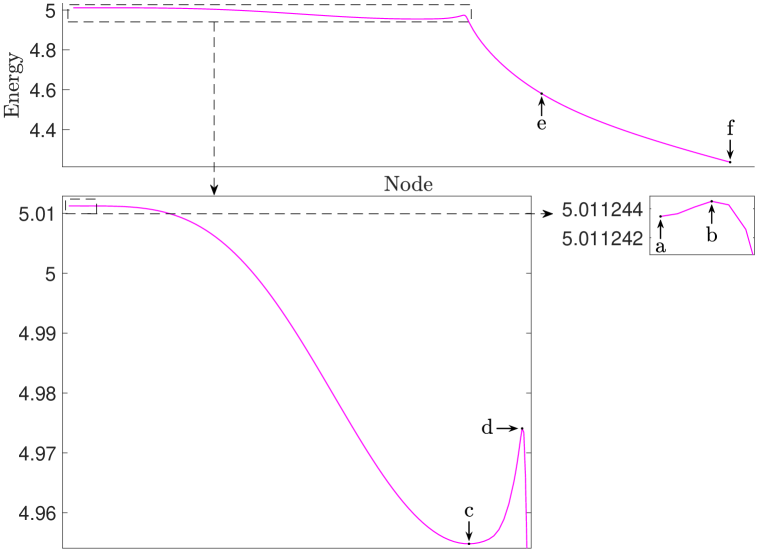
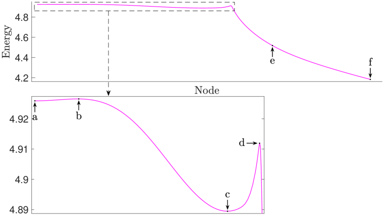
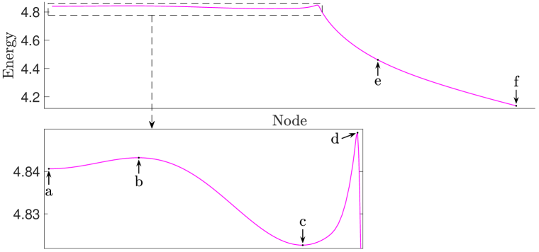
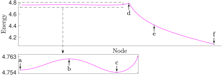
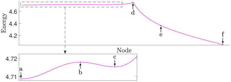
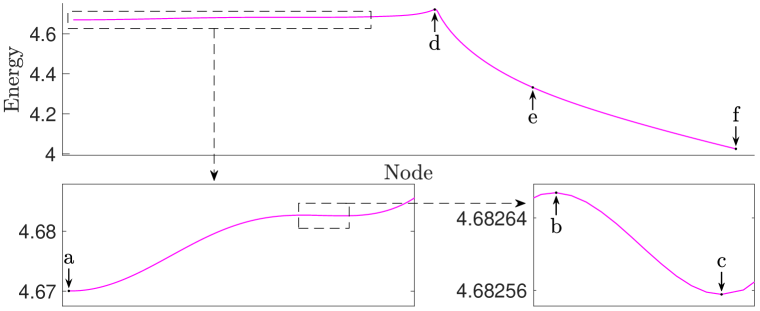
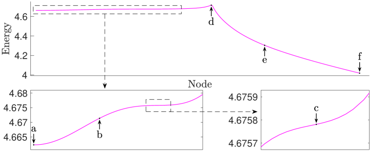
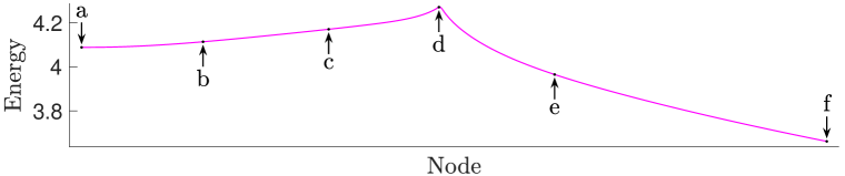
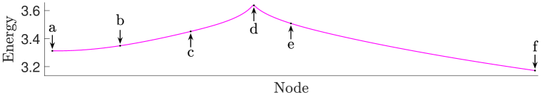
Appendix H Simulations in 2-D under periodic boundary conditions

In this appendix we present the numerical simulations of (2) in 2-D under periodic boundary conditions. As mentioned in (3), the parameter $\widetilde{\chi}$ refers to $\tilde{\gamma}\big{(}\omega|D|/\pi\big{)}^{3/2}/12$, where we choose $\omega|D|=0.1$. The results here are similar to those under no boundary conditions (in Section 4.4), and we expect the former to converge to the latter as $\omega\rightarrow 0$.

We numerically study the pACOK dynamics with the initial value resembling the indicator function of a disk. According to our simulation results, there is a critical value $\raisebox{2.0pt}{$\widetilde{\chi}$}_{*}\in(1.225,1.226)$ such that for $\raisebox{2.0pt}{$\widetilde{\chi}$}<\raisebox{2.0pt}{$\widetilde{\chi}$}_{*}$, the disk is stable; for $\raisebox{2.0pt}{$\widetilde{\chi}$}>\raisebox{2.0pt}{$\widetilde{\chi}$}_{*}$, the disk is unstable and will eventually deform into an eye-mask shaped local minimizer. We use such an eye-mask shaped local minimizer as the initial value, and numerically solve the pACOK dynamics with a larger or smaller $\widetilde{\chi}$. In this way we can track this bifurcation branch up and down. Our numerical results show that this bifurcation branch disappears at $\raisebox{2.0pt}{$\widetilde{\chi}$}=\raisebox{2.0pt}{$\widetilde{\chi}$}_{4}\in(1.182,1.184)$ through a saddle-node bifurcation.

We use the string method to compute the minimum energy paths. The is a critical value $\raisebox{2.0pt}{$\widetilde{\chi}$}_{3}\in(0.545,0.556)$ such that for $\raisebox{2.0pt}{$\widetilde{\chi}$}<\raisebox{2.0pt}{$\widetilde{\chi}$}_{3}$, the computed minimum energy path of fission is unstable against mass-asymmetric perturbations. After sufficiently many iterations in the string method, such a fission path will eventually converge to another minimum energy path called the spallation path.

Refer to caption

aRefer to captionRefer to captiona\overset{\includegraphics[width=53.0pt]{images/Periodic2D/gamma=10.57/a.png}}{\begin{minipage}[t][0pt][b]{24.0pt}\hskip 10.0pta\end{minipage}} bRefer to captionRefer to captionb\overset{\includegraphics[width=53.0pt]{images/Periodic2D/gamma=10.57/b.png}}{\begin{minipage}[t][0pt][b]{24.0pt}\hskip 10.0ptb\end{minipage}} cRefer to captionRefer to captionc\overset{\includegraphics[width=53.0pt]{images/Periodic2D/gamma=10.57/c.png}}{\begin{minipage}[t][0pt][b]{24.0pt}\hskip 10.0ptc\end{minipage}} dRefer to captionRefer to captiond\overset{\includegraphics[width=53.0pt]{images/Periodic2D/gamma=10.57/d.png}}{\begin{minipage}[t][0pt][b]{24.0pt}\hskip 10.0ptd\end{minipage}} eRefer to captionRefer to captione\overset{\includegraphics[width=53.0pt]{images/Periodic2D/gamma=10.57/e.png}}{\begin{minipage}[t][0pt][b]{24.0pt}\hskip 10.0pte\end{minipage}}

fRefer to captionRefer to captionf\overset{\includegraphics[width=53.0pt]{images/Periodic2D/gamma=10.57/f.png}}{\begin{minipage}[t][0pt][b]{24.0pt}\hskip 10.0ptf\end{minipage}} gRefer to captionRefer to captiong\overset{\includegraphics[width=53.0pt]{images/Periodic2D/gamma=10.57/g.png}}{\begin{minipage}[t][0pt][b]{24.0pt}\hskip 10.0ptg\end{minipage}} hRefer to captionRefer to captionh\overset{\includegraphics[width=53.0pt]{images/Periodic2D/gamma=10.57/h.png}}{\begin{minipage}[t][0pt][b]{24.0pt}\hskip 10.0pth\end{minipage}} iRefer to captionRefer to captioni\overset{\includegraphics[width=53.0pt]{images/Periodic2D/gamma=10.57/i.png}}{\begin{minipage}[t][0pt][b]{24.0pt}\hskip 10.0pti\end{minipage}} jRefer to captionRefer to captionj\overset{\includegraphics[width=53.0pt]{images/Periodic2D/gamma=10.57/j.png}}{\begin{minipage}[t][0pt][b]{24.0pt}\hskip 10.0ptj\end{minipage}}

Figure 44: Minimum energy paths ($\raisebox{2.0pt}{$\widetilde{\chi}$}\!=\!1.225$). Transition states: b, d and g. Local minimizers: a, c and j.
Refer to caption

aRefer to captionRefer to captiona\overset{\includegraphics[width=53.0pt]{images/Periodic2D/gamma=10.5/a.png}}{\begin{minipage}[t][0pt][b]{24.0pt}\hskip 10.0pta\end{minipage}} bRefer to captionRefer to captionb\overset{\includegraphics[width=53.0pt]{images/Periodic2D/gamma=10.5/b.png}}{\begin{minipage}[t][0pt][b]{24.0pt}\hskip 10.0ptb\end{minipage}} cRefer to captionRefer to captionc\overset{\includegraphics[width=53.0pt]{images/Periodic2D/gamma=10.5/c.png}}{\begin{minipage}[t][0pt][b]{24.0pt}\hskip 10.0ptc\end{minipage}} dRefer to captionRefer to captiond\overset{\includegraphics[width=53.0pt]{images/Periodic2D/gamma=10.5/d.png}}{\begin{minipage}[t][0pt][b]{24.0pt}\hskip 10.0ptd\end{minipage}} eRefer to captionRefer to captione\overset{\includegraphics[width=53.0pt]{images/Periodic2D/gamma=10.5/e.png}}{\begin{minipage}[t][0pt][b]{24.0pt}\hskip 10.0pte\end{minipage}}

fRefer to captionRefer to captionf\overset{\includegraphics[width=53.0pt]{images/Periodic2D/gamma=10.5/f.png}}{\begin{minipage}[t][0pt][b]{24.0pt}\hskip 10.0ptf\end{minipage}} gRefer to captionRefer to captiong\overset{\includegraphics[width=53.0pt]{images/Periodic2D/gamma=10.5/g.png}}{\begin{minipage}[t][0pt][b]{24.0pt}\hskip 10.0ptg\end{minipage}} hRefer to captionRefer to captionh\overset{\includegraphics[width=53.0pt]{images/Periodic2D/gamma=10.5/h.png}}{\begin{minipage}[t][0pt][b]{24.0pt}\hskip 10.0pth\end{minipage}} iRefer to captionRefer to captioni\overset{\includegraphics[width=53.0pt]{images/Periodic2D/gamma=10.5/i.png}}{\begin{minipage}[t][0pt][b]{24.0pt}\hskip 10.0pti\end{minipage}} jRefer to captionRefer to captionj\overset{\includegraphics[width=53.0pt]{images/Periodic2D/gamma=10.5/j.png}}{\begin{minipage}[t][0pt][b]{24.0pt}\hskip 10.0ptj\end{minipage}}

Figure 45: Minimum energy paths ($\raisebox{2.0pt}{$\widetilde{\chi}$}\!=\!1.217$). Transition states: b, d and g. Local minimizers: a, c and j.
Refer to caption

aRefer to captionRefer to captiona\overset{\includegraphics[width=53.0pt]{images/Periodic2D/gamma=10.4/a.png}}{\begin{minipage}[t][0pt][b]{24.0pt}\hskip 10.0pta\end{minipage}} bRefer to captionRefer to captionb\overset{\includegraphics[width=53.0pt]{images/Periodic2D/gamma=10.4/b.png}}{\begin{minipage}[t][0pt][b]{24.0pt}\hskip 10.0ptb\end{minipage}} cRefer to captionRefer to captionc\overset{\includegraphics[width=53.0pt]{images/Periodic2D/gamma=10.4/c.png}}{\begin{minipage}[t][0pt][b]{24.0pt}\hskip 10.0ptc\end{minipage}} dRefer to captionRefer to captiond\overset{\includegraphics[width=53.0pt]{images/Periodic2D/gamma=10.4/d.png}}{\begin{minipage}[t][0pt][b]{24.0pt}\hskip 10.0ptd\end{minipage}} eRefer to captionRefer to captione\overset{\includegraphics[width=53.0pt]{images/Periodic2D/gamma=10.4/e.png}}{\begin{minipage}[t][0pt][b]{24.0pt}\hskip 10.0pte\end{minipage}}

fRefer to captionRefer to captionf\overset{\includegraphics[width=53.0pt]{images/Periodic2D/gamma=10.4/f.png}}{\begin{minipage}[t][0pt][b]{24.0pt}\hskip 10.0ptf\end{minipage}} gRefer to captionRefer to captiong\overset{\includegraphics[width=53.0pt]{images/Periodic2D/gamma=10.4/g.png}}{\begin{minipage}[t][0pt][b]{24.0pt}\hskip 10.0ptg\end{minipage}} hRefer to captionRefer to captionh\overset{\includegraphics[width=53.0pt]{images/Periodic2D/gamma=10.4/h.png}}{\begin{minipage}[t][0pt][b]{24.0pt}\hskip 10.0pth\end{minipage}} iRefer to captionRefer to captioni\overset{\includegraphics[width=53.0pt]{images/Periodic2D/gamma=10.4/i.png}}{\begin{minipage}[t][0pt][b]{24.0pt}\hskip 10.0pti\end{minipage}} jRefer to captionRefer to captionj\overset{\includegraphics[width=53.0pt]{images/Periodic2D/gamma=10.4/j.png}}{\begin{minipage}[t][0pt][b]{24.0pt}\hskip 10.0ptj\end{minipage}}

Figure 46: Minimum energy paths ($\raisebox{2.0pt}{$\widetilde{\chi}$}\!=\!1.206$). Transition states: b, d and g. Local minimizers: a, c and j.
Refer to caption

aRefer to captionRefer to captiona\overset{\includegraphics[width=53.0pt]{images/Periodic2D/gamma=10.3/a.png}}{\begin{minipage}[t][0pt][b]{24.0pt}\hskip 10.0pta\end{minipage}} bRefer to captionRefer to captionb\overset{\includegraphics[width=53.0pt]{images/Periodic2D/gamma=10.3/b.png}}{\begin{minipage}[t][0pt][b]{24.0pt}\hskip 10.0ptb\end{minipage}} cRefer to captionRefer to captionc\overset{\includegraphics[width=53.0pt]{images/Periodic2D/gamma=10.3/c.png}}{\begin{minipage}[t][0pt][b]{24.0pt}\hskip 10.0ptc\end{minipage}} dRefer to captionRefer to captiond\overset{\includegraphics[width=53.0pt]{images/Periodic2D/gamma=10.3/d.png}}{\begin{minipage}[t][0pt][b]{24.0pt}\hskip 10.0ptd\end{minipage}} eRefer to captionRefer to captione\overset{\includegraphics[width=53.0pt]{images/Periodic2D/gamma=10.3/e.png}}{\begin{minipage}[t][0pt][b]{24.0pt}\hskip 10.0pte\end{minipage}}

fRefer to captionRefer to captionf\overset{\includegraphics[width=53.0pt]{images/Periodic2D/gamma=10.3/f.png}}{\begin{minipage}[t][0pt][b]{24.0pt}\hskip 10.0ptf\end{minipage}} gRefer to captionRefer to captiong\overset{\includegraphics[width=53.0pt]{images/Periodic2D/gamma=10.3/g.png}}{\begin{minipage}[t][0pt][b]{24.0pt}\hskip 10.0ptg\end{minipage}} hRefer to captionRefer to captionh\overset{\includegraphics[width=53.0pt]{images/Periodic2D/gamma=10.3/h.png}}{\begin{minipage}[t][0pt][b]{24.0pt}\hskip 10.0pth\end{minipage}} iRefer to captionRefer to captioni\overset{\includegraphics[width=53.0pt]{images/Periodic2D/gamma=10.3/i.png}}{\begin{minipage}[t][0pt][b]{24.0pt}\hskip 10.0pti\end{minipage}} jRefer to captionRefer to captionj\overset{\includegraphics[width=53.0pt]{images/Periodic2D/gamma=10.3/j.png}}{\begin{minipage}[t][0pt][b]{24.0pt}\hskip 10.0ptj\end{minipage}}

Figure 47: Minimum energy paths ($\raisebox{2.0pt}{$\widetilde{\chi}$}\!=\!1.194$). Transition states: b, d and g. Local minimizers: a, c and j.
Refer to caption

aRefer to captionRefer to captiona\overset{\includegraphics[width=53.0pt]{images/Periodic2D/gamma=10.21/a.png}}{\begin{minipage}[t][0pt][b]{24.0pt}\hskip 10.0pta\end{minipage}} bRefer to captionRefer to captionb\overset{\includegraphics[width=53.0pt]{images/Periodic2D/gamma=10.21/b.png}}{\begin{minipage}[t][0pt][b]{24.0pt}\hskip 10.0ptb\end{minipage}} cRefer to captionRefer to captionc\overset{\includegraphics[width=53.0pt]{images/Periodic2D/gamma=10.21/c.png}}{\begin{minipage}[t][0pt][b]{24.0pt}\hskip 10.0ptc\end{minipage}} dRefer to captionRefer to captiond\overset{\includegraphics[width=53.0pt]{images/Periodic2D/gamma=10.21/d.png}}{\begin{minipage}[t][0pt][b]{24.0pt}\hskip 10.0ptd\end{minipage}} eRefer to captionRefer to captione\overset{\includegraphics[width=53.0pt]{images/Periodic2D/gamma=10.21/e.png}}{\begin{minipage}[t][0pt][b]{24.0pt}\hskip 10.0pte\end{minipage}}

fRefer to captionRefer to captionf\overset{\includegraphics[width=53.0pt]{images/Periodic2D/gamma=10.21/f.png}}{\begin{minipage}[t][0pt][b]{24.0pt}\hskip 10.0ptf\end{minipage}} gRefer to captionRefer to captiong\overset{\includegraphics[width=53.0pt]{images/Periodic2D/gamma=10.21/g.png}}{\begin{minipage}[t][0pt][b]{24.0pt}\hskip 10.0ptg\end{minipage}} hRefer to captionRefer to captionh\overset{\includegraphics[width=53.0pt]{images/Periodic2D/gamma=10.21/h.png}}{\begin{minipage}[t][0pt][b]{24.0pt}\hskip 10.0pth\end{minipage}} iRefer to captionRefer to captioni\overset{\includegraphics[width=53.0pt]{images/Periodic2D/gamma=10.21/i.png}}{\begin{minipage}[t][0pt][b]{24.0pt}\hskip 10.0pti\end{minipage}} jRefer to captionRefer to captionj\overset{\includegraphics[width=53.0pt]{images/Periodic2D/gamma=10.21/j.png}}{\begin{minipage}[t][0pt][b]{24.0pt}\hskip 10.0ptj\end{minipage}}

Figure 48: Minimum energy paths ($\raisebox{2.0pt}{$\widetilde{\chi}$}\!=\!1.184$). Transition states: b, d and g. Local minimizers: a, c and j.
Refer to caption

aRefer to captionRefer to captiona\overset{\includegraphics[width=53.0pt]{images/Periodic2D/gamma=10.2/a.png}}{\begin{minipage}[t][0pt][b]{24.0pt}\hskip 10.0pta\end{minipage}} bRefer to captionRefer to captionb\overset{\includegraphics[width=53.0pt]{images/Periodic2D/gamma=10.2/b.png}}{\begin{minipage}[t][0pt][b]{24.0pt}\hskip 10.0ptb\end{minipage}} cRefer to captionRefer to captionc\overset{\includegraphics[width=53.0pt]{images/Periodic2D/gamma=10.2/c.png}}{\begin{minipage}[t][0pt][b]{24.0pt}\hskip 10.0ptc\end{minipage}} dRefer to captionRefer to captiond\overset{\includegraphics[width=53.0pt]{images/Periodic2D/gamma=10.2/d.png}}{\begin{minipage}[t][0pt][b]{24.0pt}\hskip 10.0ptd\end{minipage}} eRefer to captionRefer to captione\overset{\includegraphics[width=53.0pt]{images/Periodic2D/gamma=10.2/e.png}}{\begin{minipage}[t][0pt][b]{24.0pt}\hskip 10.0pte\end{minipage}}

fRefer to captionRefer to captionf\overset{\includegraphics[width=53.0pt]{images/Periodic2D/gamma=10.2/f.png}}{\begin{minipage}[t][0pt][b]{24.0pt}\hskip 10.0ptf\end{minipage}} gRefer to captionRefer to captiong\overset{\includegraphics[width=53.0pt]{images/Periodic2D/gamma=10.2/g.png}}{\begin{minipage}[t][0pt][b]{24.0pt}\hskip 10.0ptg\end{minipage}} hRefer to captionRefer to captionh\overset{\includegraphics[width=53.0pt]{images/Periodic2D/gamma=10.2/h.png}}{\begin{minipage}[t][0pt][b]{24.0pt}\hskip 10.0pth\end{minipage}} iRefer to captionRefer to captioni\overset{\includegraphics[width=53.0pt]{images/Periodic2D/gamma=10.2/i.png}}{\begin{minipage}[t][0pt][b]{24.0pt}\hskip 10.0pti\end{minipage}} jRefer to captionRefer to captionj\overset{\includegraphics[width=53.0pt]{images/Periodic2D/gamma=10.2/j.png}}{\begin{minipage}[t][0pt][b]{24.0pt}\hskip 10.0ptj\end{minipage}}

Figure 49: Minimum energy paths ($\raisebox{2.0pt}{$\widetilde{\chi}$}\!=\!1.182$). Transition states: d and g.
Refer to caption

aRefer to captionRefer to captiona\overset{\includegraphics[width=53.0pt]{images/Periodic2D/gamma=8/a.png}}{\begin{minipage}[t][0pt][b]{24.0pt}\hskip 10.0pta\end{minipage}} bRefer to captionRefer to captionb\overset{\includegraphics[width=53.0pt]{images/Periodic2D/gamma=8/b.png}}{\begin{minipage}[t][0pt][b]{24.0pt}\hskip 10.0ptb\end{minipage}} cRefer to captionRefer to captionc\overset{\includegraphics[width=53.0pt]{images/Periodic2D/gamma=8/c.png}}{\begin{minipage}[t][0pt][b]{24.0pt}\hskip 10.0ptc\end{minipage}} dRefer to captionRefer to captiond\overset{\includegraphics[width=53.0pt]{images/Periodic2D/gamma=8/d.png}}{\begin{minipage}[t][0pt][b]{24.0pt}\hskip 10.0ptd\end{minipage}} eRefer to captionRefer to captione\overset{\includegraphics[width=53.0pt]{images/Periodic2D/gamma=8/e.png}}{\begin{minipage}[t][0pt][b]{24.0pt}\hskip 10.0pte\end{minipage}}

fRefer to captionRefer to captionf\overset{\includegraphics[width=53.0pt]{images/Periodic2D/gamma=8/f.png}}{\begin{minipage}[t][0pt][b]{24.0pt}\hskip 10.0ptf\end{minipage}} gRefer to captionRefer to captiong\overset{\includegraphics[width=53.0pt]{images/Periodic2D/gamma=8/g.png}}{\begin{minipage}[t][0pt][b]{24.0pt}\hskip 10.0ptg\end{minipage}} hRefer to captionRefer to captionh\overset{\includegraphics[width=53.0pt]{images/Periodic2D/gamma=8/h.png}}{\begin{minipage}[t][0pt][b]{24.0pt}\hskip 10.0pth\end{minipage}} iRefer to captionRefer to captioni\overset{\includegraphics[width=53.0pt]{images/Periodic2D/gamma=8/i.png}}{\begin{minipage}[t][0pt][b]{24.0pt}\hskip 10.0pti\end{minipage}} jRefer to captionRefer to captionj\overset{\includegraphics[width=53.0pt]{images/Periodic2D/gamma=8/j.png}}{\begin{minipage}[t][0pt][b]{24.0pt}\hskip 10.0ptj\end{minipage}}

Figure 50: Minimum energy paths ($\raisebox{2.0pt}{$\widetilde{\chi}$}\!=\!0.927$). Transition states: d and g.
Refer to caption

aRefer to captionRefer to captiona\overset{\includegraphics[width=53.0pt]{images/Periodic2D/gamma=6/a.png}}{\begin{minipage}[t][0pt][b]{24.0pt}\hskip 10.0pta\end{minipage}} bRefer to captionRefer to captionb\overset{\includegraphics[width=53.0pt]{images/Periodic2D/gamma=6/b.png}}{\begin{minipage}[t][0pt][b]{24.0pt}\hskip 10.0ptb\end{minipage}} cRefer to captionRefer to captionc\overset{\includegraphics[width=53.0pt]{images/Periodic2D/gamma=6/c.png}}{\begin{minipage}[t][0pt][b]{24.0pt}\hskip 10.0ptc\end{minipage}} dRefer to captionRefer to captiond\overset{\includegraphics[width=53.0pt]{images/Periodic2D/gamma=6/d.png}}{\begin{minipage}[t][0pt][b]{24.0pt}\hskip 10.0ptd\end{minipage}} eRefer to captionRefer to captione\overset{\includegraphics[width=53.0pt]{images/Periodic2D/gamma=6/e.png}}{\begin{minipage}[t][0pt][b]{24.0pt}\hskip 10.0pte\end{minipage}}

fRefer to captionRefer to captionf\overset{\includegraphics[width=53.0pt]{images/Periodic2D/gamma=6/f.png}}{\begin{minipage}[t][0pt][b]{24.0pt}\hskip 10.0ptf\end{minipage}} gRefer to captionRefer to captiong\overset{\includegraphics[width=53.0pt]{images/Periodic2D/gamma=6/g.png}}{\begin{minipage}[t][0pt][b]{24.0pt}\hskip 10.0ptg\end{minipage}} hRefer to captionRefer to captionh\overset{\includegraphics[width=53.0pt]{images/Periodic2D/gamma=6/h.png}}{\begin{minipage}[t][0pt][b]{24.0pt}\hskip 10.0pth\end{minipage}} iRefer to captionRefer to captioni\overset{\includegraphics[width=53.0pt]{images/Periodic2D/gamma=6/i.png}}{\begin{minipage}[t][0pt][b]{24.0pt}\hskip 10.0pti\end{minipage}} jRefer to captionRefer to captionj\overset{\includegraphics[width=53.0pt]{images/Periodic2D/gamma=6/j.png}}{\begin{minipage}[t][0pt][b]{24.0pt}\hskip 10.0ptj\end{minipage}}

Figure 51: Minimum energy paths ($\raisebox{2.0pt}{$\widetilde{\chi}$}\!=\!0.696$). Transition states: d and h.
Refer to caption

aRefer to captionRefer to captiona\overset{\includegraphics[width=53.0pt]{images/Periodic2D/gamma=4.8/a.png}}{\begin{minipage}[t][0pt][b]{24.0pt}\hskip 10.0pta\end{minipage}} bRefer to captionRefer to captionb\overset{\includegraphics[width=53.0pt]{images/Periodic2D/gamma=4.8/b.png}}{\begin{minipage}[t][0pt][b]{24.0pt}\hskip 10.0ptb\end{minipage}} cRefer to captionRefer to captionc\overset{\includegraphics[width=53.0pt]{images/Periodic2D/gamma=4.8/c.png}}{\begin{minipage}[t][0pt][b]{24.0pt}\hskip 10.0ptc\end{minipage}} dRefer to captionRefer to captiond\overset{\includegraphics[width=53.0pt]{images/Periodic2D/gamma=4.8/d.png}}{\begin{minipage}[t][0pt][b]{24.0pt}\hskip 10.0ptd\end{minipage}} eRefer to captionRefer to captione\overset{\includegraphics[width=53.0pt]{images/Periodic2D/gamma=4.8/e.png}}{\begin{minipage}[t][0pt][b]{24.0pt}\hskip 10.0pte\end{minipage}}

fRefer to captionRefer to captionf\overset{\includegraphics[width=53.0pt]{images/Periodic2D/gamma=4.8/f.png}}{\begin{minipage}[t][0pt][b]{24.0pt}\hskip 10.0ptf\end{minipage}} gRefer to captionRefer to captiong\overset{\includegraphics[width=53.0pt]{images/Periodic2D/gamma=4.8/g.png}}{\begin{minipage}[t][0pt][b]{24.0pt}\hskip 10.0ptg\end{minipage}} hRefer to captionRefer to captionh\overset{\includegraphics[width=53.0pt]{images/Periodic2D/gamma=4.8/h.png}}{\begin{minipage}[t][0pt][b]{24.0pt}\hskip 10.0pth\end{minipage}} iRefer to captionRefer to captioni\overset{\includegraphics[width=53.0pt]{images/Periodic2D/gamma=4.8/i.png}}{\begin{minipage}[t][0pt][b]{24.0pt}\hskip 10.0pti\end{minipage}} jRefer to captionRefer to captionj\overset{\includegraphics[width=53.0pt]{images/Periodic2D/gamma=4.8/j.png}}{\begin{minipage}[t][0pt][b]{24.0pt}\hskip 10.0ptj\end{minipage}}

Figure 52: Minimum energy paths ($\raisebox{2.0pt}{$\widetilde{\chi}$}\!=\!0.556$). Transition states: d and h.

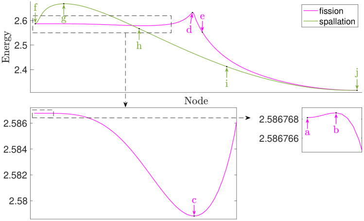
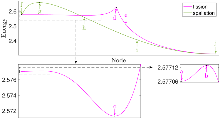
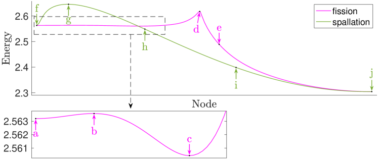
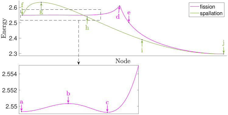
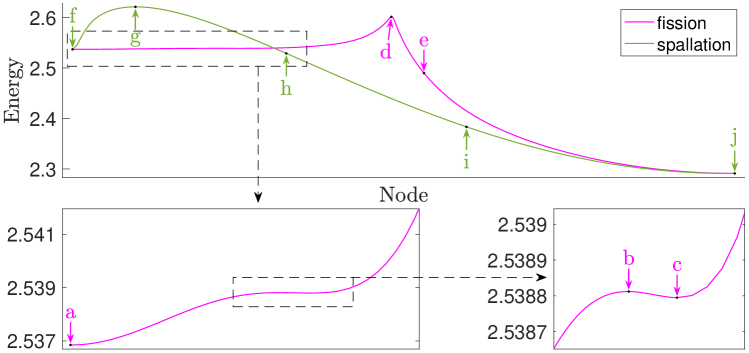
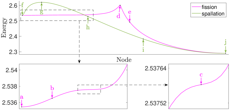
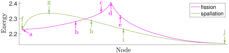
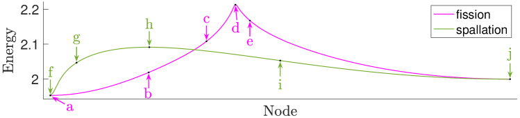
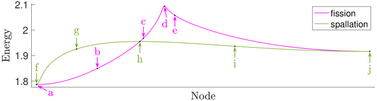
Appendix I Simulations in 3-D of torus-like equilibria

In this appendix, we present torus-like equilibria in 3-D under no boundary conditions. A portion (where $\chi$ is large enough) of this bifurcation branch has already been found in [59]. As mentioned in Section 5, a cylinder with a height larger than its circumference is unstable under surface tension. Therefore we expect the torus-like equilibria to be unstable (see also [60]). (In contrast, a 2-D strip is stable under surface tension, so an annulus might be stable in 2-D [40, Theorem 2.2]. Similarly, we expect a spherical shell to be stable in 3-D. However, the spherical shell is reported to be unstable [54, Page 981], which may seem surprising at first, but such an instability can be understood as the consequence of the Coulomb repulsive term.)

In order to overcome the instability of the torus-like equilibrium, we employ the following technique to maintain the axisymmetry of the shape: after every a few (e.g., 500) iterations in the pACOK dynamics, rotate it by $30^{\circ},\,60^{\circ},\,90^{\circ},\,\cdots,\,360^{\circ}$, then take the average in the sense of superposition. In our simulations, there exists a $\raisebox{2.0pt}{$\widetilde{\chi}$}_{4}\in(0.968,0.969)$, such that for $\raisebox{2.0pt}{$\widetilde{\chi}$}<\raisebox{2.0pt}{$\widetilde{\chi}$}_{4}$, the torus will eventually converge to a ball, so we suspect that the torus-like equilibrium disappears through a saddle-node bifurcation at $\raisebox{2.0pt}{$\chi$}=\raisebox{2.0pt}{$\chi$}_{4}$. We use $\raisebox{2.0pt}{$\widetilde{\chi}$}_{4}/\raisebox{2.0pt}{$\widetilde{\chi}$}_{*}\approx 0.972$ to estimate $\raisebox{2.0pt}{$\chi$}_{4}$. For $\raisebox{2.0pt}{$\widetilde{\chi}$}>\raisebox{2.0pt}{$\widetilde{\chi}$}_{4}$, our numerical results are shown in Figure 53.

0.969Refer to captionRefer to caption0.969\overset{\includegraphics[width=103.6pt,bb=0 0 569 344]{images/BifurcationBranch/t7.81.png}}{0.969} 0.992Refer to captionRefer to caption0.992\overset{\includegraphics[width=103.6pt,bb=0 0 569 344]{images/BifurcationBranch/t8.png}}{0.992} 1.054Refer to captionRefer to caption1.054\overset{\includegraphics[width=103.6pt,bb=0 0 569 344]{images/BifurcationBranch/t8.5.png}}{1.054} 1.116Refer to captionRefer to caption1.116\overset{\includegraphics[width=103.6pt,bb=0 0 569 344]{images/BifurcationBranch/t9.5.png}}{1.116}
            1.178Refer to captionRefer to caption1.178\overset{\includegraphics[width=103.6pt,bb=0 0 569 344]{images/BifurcationBranch/t9.5.png}}{1.178} 1.240Refer to captionRefer to caption1.240\overset{\includegraphics[width=103.6pt,bb=0 0 569 344]{images/BifurcationBranch/t10.png}}{1.240} 1.365Refer to captionRefer to caption1.365\overset{\includegraphics[width=103.6pt,bb=0 0 569 344]{images/BifurcationBranch/t11.png}}{1.365} 1.489Refer to captionRefer to caption1.489\overset{\includegraphics[width=103.6pt,bb=0 0 569 344]{images/BifurcationBranch/t12.png}}{1.489}
1.613Refer to captionRefer to caption1.613\overset{\includegraphics[width=103.6pt,bb=0 0 569 344]{images/BifurcationBranch/t13.png}}{1.613} 1.737Refer to captionRefer to caption1.737\overset{\includegraphics[width=103.6pt,bb=0 0 569 344]{images/BifurcationBranch/t14.png}}{1.737} 1.799Refer to captionRefer to caption1.799\overset{\includegraphics[width=103.6pt,bb=0 0 569 344]{images/BifurcationBranch/t14.5.png}}{1.799} 1.811Refer to captionRefer to caption1.811\overset{\includegraphics[width=103.6pt,bb=0 0 569 344]{images/BifurcationBranch/t14.6.png}}{1.811}

Figure 53: Torus-like equilibria for various $\widetilde{\chi}$. Size of bounding box: 1.6$\times$1.6$\times$0.28125.