Geometric properties of the complete-graph Ising model in the loop representation

Abstract

The exact solution of the Ising model on the complete graph (CG) provides an important, though mean-field, insight for the theory of continuous phase transitions. Besides the original spin, the Ising model can be formulated in the Fortuin-Kasteleyn random-cluster and the loop representation, in which many geometric quantities have no correspondence in the spin representations. Using a lifted-worm irreversible algorithm, we study the CG-Ising model in the loop representation, and, based on theoretical and numerical analyses, obtain a number of exact results including volume fractal dimensions and scaling forms. Moreover, by combining with the Loop-Cluster algorithm, we demonstrate how the loop representation can provide an intuitive understanding to the recently observed rich geometric phenomena in the random-cluster representation, including the emergence of two configuration sectors, two length scales and two scaling windows.

I Introduction

The Ising model Duminil-Copin (2022) is one of the most prototypical models in statistical physics and plays an important role in the study of phase transitions and critical phenomena. It has wide applications in many fields, including material science, neuroscience and biology, etc. Given a graph (or lattice) $\mathcal{G}=(\mathcal{V},\mathcal{E})$ with the vertex set $\mathcal{V}$ and edge set $\mathcal{E}$, the Hamiltonian of the zero-field ferromagnetic Ising model reads

$$\mathcal{H}(s)=-J\sum_{ij\in\mathcal{E}}s_{i}s_{j}\;,$$ (1)

where $J>0$ is the interaction strength. The probability of a spin configuration $s\in\{-1,1\}^{\mathcal{V}}$ is given by the Gibbs measure $\pi(s)\propto e^{-\beta H(s)}$, where $\beta$ is the inverse temperature. Let $K:=\beta J$ be the reduced coupling strength, and one can set $J=1$ for convenience. On lattices $\mathbb{Z}^{d}$, it has been rigorously established that the Ising model goes through a continuous phase transition for $d\geq 2$ Onsager (1944); Aizenman and Fernández (1986); Aizenman et al. (2015).

In addition to its spin representation in Eq. (1), the Ising model can be formulated in two other geometric representations, the loop representation and the Fortuin-Kasteleyn (FK) bond representation. Here, we provide a brief overview of these two representations for clarity. In 1941, Van der Waerden proposed a high-temperature expansion trick van der Waerden (1941) for the Ising model, where the statistical weight for each interaction term is rewritten as $\exp(Ks_{i}s_{j})=\cosh{K}(1+s_{i}s_{j}\tanh{K})$. Further, an auxilliary variable $f_{ij}=0,1$ is introduced such that the second term, $s_{i}s_{j}\tanh K$, is geometrically represented by an occupied bond $f_{ij}=1$, and the first term corresponds to an empty bond $f_{ij}=0$. Then, the spin degrees of freedom can be integrated out by calculating the partition function $\mathcal{Z}_{\rm{spin}}=\sum_{s}e^{-\beta\mathcal{H}(s)}$, leading to the summation of geometric configurations of bond variables $f$. Due to the $\mathbb{Z}_{2}$ symmetry of the Ising spins, non-zero contributions to the partition function come only from those configurations $\mathcal{F}$, in which any vertex is incident to an even number of occupied bonds. Such a configuration is composed of loops (also called currents or flows). In graph theory, such a loop configuration is referred to an Eulerian graph or an even graph. Let ${\rm even}(\mathcal{G})$ be the set of loop configurations on $\mathcal{G}$. Then loop Ising model is defined by giving any $\mathcal{F}$ the probability measure

$$\pi(\mathcal{F})\propto w^{|\mathcal{F}|}\delta_{\mathcal{F}\in{\rm even}(\mathcal{G})}\;,$$ (2)

where $|\mathcal{F}|$ represents the total number of occupied bonds, the bond weight is $w=\tanh{K}$ and $\delta_{\mathcal{F}\in{\rm even}(\mathcal{G})}$ is an indicator function that ensures that any graph $\mathcal{F}$ descried by the flow variables is an even graph. Apart from the Eulerian requirement, the probability measure (2) would describe the standard bond percolation, and, thus, the loop representation of the Ising model can be regarded as the Eulerian bond percolation model. Other names for this representation include the random-current modelDuminil-Copin (2016), random even graphGrimmett and Janson (2007) or the flow representation of the Ising model.

The $Q$-state Potts model Wu (1982), in which the value of spins can take $\sigma\in\{0,1,\cdots,Q-1\}$, is a generalization of the Ising model and has the latter as a special case of $Q=2$. In 1969, Fortuin and Kasteleyn established an exact mapping between the Potts model and a geometric model, called the random-cluster (RC) model Fortuin and Kasteleyn (1972); Grimmett (2006). Similar to loop configuration, for each edge $ij$, a binary variable $b_{ij}\in\{0,1\}$ is defined to represent whether the edge is occupied by a bond ($b_{ij}=1$) or empty ($b_{ij}=0$), but no Eulerian constraint is required in the FK configurations. The $Q$-state RC model is defined by choosing a spanning subgraph $\mathcal{A}\subseteq\mathcal{G}$ with the probability

$$\pi(\mathcal{A})\propto Q^{k(\mathcal{A})}p^{|\mathcal{A}|}(1-p)^{|\mathcal{E}|-|\mathcal{A}|},$$ (3)

where $p$ is the bond occupation probability and $k(\mathcal{A})$ is the number of connected components (or clusters) on $\mathcal{A}$. The case $Q=2$ with $p=1-e^{-2K}$ corresponds to the Ising model, or known as the FK Ising model, where $K$ is the reduced coupling strength mentioned before.

These three representations are illustrated in Fig. 1.

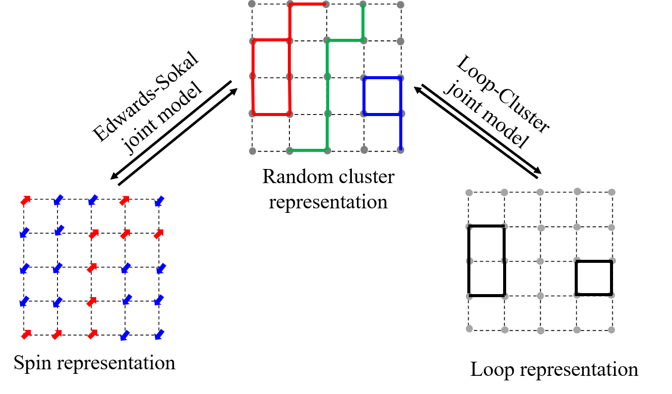
Figure 1: Three representations of the Ising model. The random-cluster representation is depicted with lines of different colors indicating different clusters. The Edwards-Sokal joint model couples the spin and random-cluster representations, while the Loop-Cluster joint model couples the loop and random-cluster representations.

In comparison to the spin representation, geometric representations enable the definition of a broader range of geometric observables, many of which have no corresponding analogs in the spin representation, leading to a wealth of phenomena. For example, while the upper critical dimension of the spin Ising model has been known to be $d_{c}=4$ since the 1970s, recent studies argued that the FK-Ising model simultaneously has two upper critical dimensions, namely $d_{c}=4$ and $d_{p}=6$ Fang et al. (2022a, b), where the dimension $d_{p}=6$ cannot be observed in the spin representation. Moreover, the geometric representations also serve as a versatile platform for conformal field theory Francesco et al. (2012) and stochastic Loewner evolution Kager and Nienhuis (2004); Cardy (2005), leading to many exact results in two dimensions. In mathematical physics, the geometric representations play a crucial role in the rigorous study of phase transitions for the Ising model in dimensions $d\geq 3$ Aizenman and Fernández (1986); Aizenman et al. (2015) and the triviality of criticality for $d=4$ Aizenman and Duminil-Copin (2021).

Advanced Monte Carlo methods have also benefited from the geometric representations. A notable example is the highly efficient Swendsen-Wang cluster algorithm Swendsen and Wang (1987), passing back and forth between the FK and the spin configurations. The Edwards-Sokal joint model Edwards and Sokal (1988), in which the spin and FK-bond variables are coupled together, establishes a connection between the FK and the spin representations and offers a concise understanding to the Swendsen-Wang algorithm.

Another example is the Loop-Cluster (LC) algorithm, which passes back and forth between the FK and loop representations via the LC joint model Zhang et al. (2020). A configuration of the LC joint model can be interpreted as a superposition of a FK and a loop configuration, where each edge is associated with both a FK bond and a flow variable. For the Ising model ($Q=2$), the probability measure of an LC joint configuration is defined as follows,

$$\pi(\mathcal{A},\mathcal{F})\propto\left(\frac{p}{2}\right)^{|\mathcal{F}|}\left(\frac{p}{2}\right)^{|\mathcal{A}|-|\mathcal{F}|}(1-p)^{|\mathcal{E}|-|\mathcal{A}|}\delta_{\mathcal{F}\in{\rm even}(\mathcal{G})}.$$ (4)

More specifically, there are four edge states in the LC joint model:

$$\mathcal{L}_{1}:b_{ij}=0,f_{ij}=0;$$

$$\mathcal{L}_{2}:b_{ij}=1,f_{ij}=0;$$

$$\mathcal{L}_{3}:b_{ij}=1,f_{ij}=1;$$

$$\mathcal{L}_{4}:b_{ij}=0,f_{ij}=1.$$ (5)

The edge state $\mathcal{L}_{4}$, i.e, with an empty FK bond and an occupied loop bond, is forbidden. From Eq. (4) the probabilities of other edge states read:

$$P(\mathcal{L}_{1})=1-p;\ \ P(\mathcal{L}_{2})=\frac{p}{2};\ \ P(\mathcal{L}_{3})=\frac{p}{2}.$$ (6)

From a given loop configuration $\{f\}$, the LC algorithm generates a stochastic FK bond configuration $\{b\}$ by a local bond-placing process. To be specific, for each nonzero flow $f_{ij}=1$, one sets $b_{ij}=1$; for each empty flow $f_{ij}=0$, one independently sets $b_{ij}=1$ with probability

$$w^{\prime}=\frac{\frac{p}{2}}{\frac{p}{2}+(1-p)}=\tanh{K},$$ (7)

which equals to $w$, or $b_{ij}=0$, otherwise. In other words, the process from the loop to the FK representation is basically to add occupied bonds to those edges of empty flow via a process of standard bond percolation with probability $w$.

In statistical mechanics, it is of particular interest to study models on the complete graph (CG) because it is usually more tractable and provides important insights to understand critical behaviors on high-dimensional tori. On the CG, each vertex is connected to all others, and thus in order to obtain an extensive system, the coupling strength $K$ must be rescaled by its volume $V$. For the FK-Ising model on the CG, it was proven that Luczak and Łuczak (2006), within a scaling window of width $O(V^{-1/2})$ around the critical point $p_{c}=1-e^{-2/V}$, the sizes of the largest and second-largest clusters scale asymptotically as $C_{1}\sim V^{3/4}$ and $C_{2}\sim\sqrt{V}\ln V$, respectively. Namely, unlike the common self-similarity observed in many other critical systems, here $C_{1}$ dominates over $C_{2}$, which indicates the system has two length (size) scales . Furthermore, the authors also proved that $C_{1},C_{2}\sim V^{2/3}$ in a wider scaling window of width $\delta p\equiv p_{c}-p=O(V^{-1/3})$ in the sub-critical side ($\delta p<0$), sharing the same scaling behavior as the CG-percolation model. Thus, the FK-Ising model on the CG has two scaling windows. Additionally, the authors in Ref. Fang et al. (2021) numerically studied the FK-Ising model on the CG and observed more interesting critical phenomena. At criticality, the cluster-number density of the FK-Ising clusters, excluding the largest one, obeys the same scaling form as that for the bond percolation on the CG. Moreover, a percolation sector was observed in the whole configuration space, which asymptotically vanishes with the rate of $V^{-1/12}$. Conditioned on being in the percolation sector, all clusters, including the largest one, have the same scaling behavior as those for the critical percolation on the CG.

In this paper, we study the CG-Ising model in the loop representation by a lifted worm update algorithm Elçi et al. (2018). The motivation is two-fold. Firstly, we aim to examine the critical scaling behaviors of the geometric clusters in the loop representation. Secondly, given that the process in the LC algorithm from the loop to the FK bond configurations is much like the conventional percolation process, we hope to gain a vivid understanding of the observed rich geometric properties for the CG-Ising model in the FK representation.

At criticality, we first study the number of occupied loop bonds (i.e., nonzero flows) $\mathcal{B}$. Based on the exact solution of the spin Ising model on the CG, we derive the mean scales as $B:=\langle\mathcal{B}\rangle\asymp\sqrt{3}\frac{\Gamma(3/4)}{\Gamma(1/4)}\sqrt{V}$, and the probability density function of $X_{B}\equiv\mathcal{B}/\sqrt{V}$ is,

$$f_{X_{B}}(x)\asymp\frac{3^{-1/4}}{2}\Gamma^{-1}(5/4)x^{-1/2}\exp\left(-\frac{1}{3}x^{2}\right)\;,$$ (8)

which is also verified by our numerics. It means that, in contrast to the FK-Ising model, the number of bonds in the loop Ising model is not extensive and has a power-law distribution till $O(\sqrt{V})$. Meanwhile, through the results of our simulations, we conjecture that the total number of flow clusters increases logarithmically as $\frac{1}{4}\ln V$, and each flow cluster is basically unicyclic. In other words, a typical loop configuration consists of an extremely dilute soup of cycles. The cluster-number density $n(s,V)$ of flow clusters, including the largest one, obeys the scaling form as

$$n(s,V)\asymp\frac{1}{2V}\;s^{-1}\tilde{n}(s/\sqrt{V})\hskip 14.22636pt\mbox{with }\;\tilde{n}(x\to 0)=1.$$ (9)

The sizes of the largest and second-largest flow clusters both scale as $F_{1},F_{2}\sim\sqrt{V}$, and, accordingly, we conjecture that the volume fractal dimension  $d_{\rm f1}=d_{\rm f2}=1/2$ holds exactly true. Unlike in the FK representation, the size distribution of the largest flow cluster displays a power-law behavior until the cut-off size $O(\sqrt{V})$, and its scaling form in the rescaled variable $X_{1}\equiv\mathcal{F}_{1}/\sqrt{V}$ reads

$$f_{X_{1}}(x)\asymp\frac{1}{2}\,x^{-1/2}\tilde{f}(x),$$ (10)

where function $\tilde{f}(x\to 0)=1$ and $\tilde{f}$ drops quickly for $x\gg 1$. Near the criticality with $\delta p$, $B$ can be demonstrated to follow the conventional finite size scaling (FSS) ansatz as $B=\sqrt{V}\tilde{B}(\delta p\sqrt{V})$ with $\tilde{B}(\cdot)$ the scaling function, and only a single scaling window of width $O(1/\sqrt{V})$ appears.

Therefore, in the loop representation, no apparent symptoms are observed for the appearance of the two length scales, of two configuration sectors, and of two scaling windows, which occur in the FK representation of the CG-Ising model. However, the loop representation provides a starting point for us to understand these rich phenomena with the LC algorithm. The density of bonds $B/V$ scales as $1/\sqrt{V}$, which suggests that the loop configurations are very dilute and become vacant as $V\to\infty$. Further, in the LC process, the probability of adding bonds to the loop configuration on the CG is $w_{c}=\tanh(1/V)\approx 1/V$, which is equal to that for the bond percolation process at criticality. Overall, the LC process can be roughly viewed as the critical bond percolation process on the CG.

More specifically, using the LC algorithm, we numerically find that the fraction of the loop bonds in the largest FK cluster tends to $1$, which means all the loop bonds belong to the largest FK cluster in the thermodynamic limit. In other words, all the other FK clusters are indeed generated by the critical percolation process in the LC algorithm. As a consequence, the emergence of two length scales in the critical FK configurations can be understood straightforwardly. Almost all loops are merged together by the newly added FK bonds, leading to a giant cluster with the volume fractal dimension $D_{\rm f1}=3/4$. The remaining clusters are effectively generated by adding bonds on the vacant space, and thus, they behave like those percolation clusters on the CGs.

It can be calculated from Eq. (8) that the probability of the vacant configuration in the loop representation scales as $V^{-1/4}$, it follows that there must exist a percolation sector decaying slowly as or more slowly than the order $V^{-1/4}$ in the FK representation. Since the volume fractal dimension of the cycle (bridge-free) in the CG percolation model is $1/3$ Huang et al. (2018) at the critical point, we conjecture that if the size of the largest loop cluster $\mathcal{F}_{1}$ is no bigger than ${\cal O}(V^{1/3})$, the corresponding FK configurations belong to the percolation sector $S^{\rm P}$. We derive that $P(S^{\rm P})$ decays as $V^{-1/12}$, providing an explanation to the previous numerical observation Fang et al. (2021) in the FK representation. We then measure the scaling of the largest FK cluster $C_{1}^{\rm P^{\prime}}$ conditioned on the original loop configuration with $\mathcal{F}_{1}\leq O(V^{1/3})$. Our data show that $C_{1}^{\rm P^{\prime}}$ scales as $V^{2/3}$, which is the same as the CG-percolation. Moreover, from the scaling behavior of $B$ near the critical point, we find out that if $\delta p=O(V^{-1/3})$ then $B$ scales the same as the number of bridge-free bonds in the percolation model. Thus, it explains the two-scaling-window behavior of the FK representation.

Recall that the rich phenomena observed in Ref. Fang et al. (2021) shows that there are strong percolation effects in the FK Ising model on the CG. These percolation effects now can be well understood from the perspective of the LC joint model. It further reveals that configurations of the FK-Ising model excluding the largest cluster are effectively equivalent to the ones of percolation at the critical point on the CG. Meanwhile, the emergence of the percolation scaling windows in the FK representation suggests that when the temperature become higher, even the scaling behavior of the largest cluster is also described by percolation.

The remainder of this paper is organized as follows. Section II summarizes the simulation details and the sampled quantities. Section III presents our theoretical analysis. Section IV contains our main numerical results. A discussion is given in Sec. V.

II Simulation & observable

II.1 Algorithm

The worm algorithm Prokof’ev and Svistunov (2001) is used to simulate the Ising model in the loop representation. The main idea of the worm algorithm is to enlarge the configuration space from close loop space to the space of the graph allowing two open ends by introducing two defects, i.e., vertices with odd degree. Configurations are updated as defects do random walks. If a defect proposes to move through a flow/loop bond, then with probability 1 the proposal is accepted and the bond is erased. If a defect is crossing an empty edge, then with probability $w$ the move is accepted and the empty edge is occupied by a bond. When two defects meet, a new loop configuration is obtained.

In Ref. Elçi et al. (2018), the authors presented an irreversible version of the worm algorithm by using the lifting technique, which leads to a critical speeding-up for observables in the simulation on the CG, with a negative dynamic exponent $z=-1/2$. In other words, between two subsequent effectively independent samplings in the Markov chain, the number of elementary updating steps is of order ${\cal O}(\sqrt{V})$ in the lifted worm algorithm. This is vanishingly small in comparison with a sweep of updates, ${\cal O}(V)$, which is a standard unit in studying the efficiency of Monte Carlo methods. The existence of this critical speeding-up, which makes the lifted worm algorithm thus far most efficient for the CG-Ising, is understandable since the number of loop bonds is also ${\cal O}(\sqrt{V})$. Therefore, we use the irreversible worm algorithm to update loop configuration here. Specifically, a lifted parameter $\lambda\in\{+,-\}$ is introduced to double the configuration space of worm update, as $\lambda=+(-)$ stands for the choice to add (delete) a bond in each step of random walk of the defect. It indicates that every time the defect moves to the next vertex, $\lambda$ determine whether the movement leads to an increase or decrease of bond on the graph, as well as the choice of the next vertex. Then we accept the update with a certain probability depending on $\lambda$ and the number of occupied bonds incident to the two defects, which is presented in Ref. Elçi et al. (2018) in details. Whenever the update is rejected, the lifted parameter $\lambda$ changes.

In addition, we implement a transformation from the loop representation to the RC representation via the LC algorithm Zhang et al. (2020) after we generate a loop configuration. The main idea of the transformation is performing a conditional probability distribution of the joint model (4). Recall that edge state $\mathcal{L}_{4}$ in Eq. (5) is forbidden, so a loop bond must also be an FK bond in the joint model. Therefore, the basic step is that: for each edge, if it has not been occupied by a bond in the loop representation, we place a bond on it with a probability $w=\tanh{(K/V)}\approx K/V$; If it has been occupied, keep it occupied. We carry out this adding bond process by an efficient cumulative method Blöte and Deng (2002).

II.2 Sample quantities

We sample the following observables in our simulations:

1. The sizes of the largest and the second-largest loop clusters denoted as $\mathcal{F}_{1}$, $\mathcal{F}_{2}$;

2. The total number of vertices in the loop clusters $\mathcal{N}_{\rm v}=\sum_{i:\mathcal{F}_{i}>1}\mathcal{F}_{i}$;

3. The number of bonds $\mathcal{B}$ in loop clusters;

4. The number of loop clusters $\mathcal{N}(s)$ with size $s$, defined as the number of loop clusters with size in $[s,s+\Delta s]$ with an appropriately chosen interval size $\Delta s$;

5. The total number of loop clusters $\mathcal{N}_{\rm k}$;

6. The indicators $\mathcal{P}^{\rm v}$,$\mathcal{P}^{(\alpha)}$. We set $\mathcal{P}^{\rm v}=1$ to record the event that the configuration is empty with bonds, $\mathcal{P}^{(\alpha)}=1$ to record if $\mathcal{F}_{1}\leq\alpha V^{\frac{1}{3}}$ with $\alpha$ is a tunable constant. Here we set $\alpha=1,2$.

From these observables, we take the ensemble average:

1. The probability of vacant configuration $P^{\rm v}=\langle\mathcal{P}^{\rm v}\rangle$;

2. The average sizes of the first- and second-largest loop cluster $F_{1}=\langle\mathcal{F}_{1}\rangle,F_{2}=\langle\mathcal{F}_{2}\rangle$ and their distribution;

3. The average number of bonds $B=\langle\mathcal{B}\rangle$ and its distribution;

4. The average number of clusters $N_{\rm k}=\langle\mathcal{N}_{\rm k}\rangle$ and the average number of vertices $N_{\rm v}=\langle\mathcal{N}_{\rm v}\rangle$;

5. The cluster-number density $n(s,V)=\frac{1}{V\Delta s}\langle\mathcal{N}(s)\rangle$, which is also called the cluster-size distribution;

6. The probability of the bond configuration in the region where the largest loop-cluster $\mathcal{F}_{1}\leq\alpha V^{1/3}$: $P(\mathcal{F}_{1}\leq\alpha V^{\frac{1}{3}})=\langle\mathcal{P}^{(\alpha)}\rangle$.

Moreover, we measure the following quantities in the FK representation:

1. The sizes of the first- and second-largest FK clusters $\mathcal{C}_{1},\mathcal{C}_{2}$ and their average $C_{1}=\langle\mathcal{C}_{1}\rangle,C_{2}=\langle\mathcal{C}_{2}\rangle$ the average size of the largest FK cluster conditioned on the origin loop configuration where $\mathcal{F}_{1}\leq 2V^{1/3}$, denote as $C_{1}^{\rm P^{\prime}}$;

2. The total size of loop clusters in the first- and second-largest FK clusters: $\mathcal{S}_{C_{1}}=\sum_{\mathcal{F}_{i}\subset\mathcal{C}_{1}}\mathcal{F}_{i}$, $\mathcal{S}_{C_{2}}=\sum_{\mathcal{F}_{i}\subset\mathcal{C}_{2}}\mathcal{F}_{i}$, and the average of them divided by the total loop cluster size $\mathcal{N}_{\rm v}$ as $n_{\rm f,1}=\frac{\langle\mathcal{S}_{C_{1}}\rangle}{\langle\mathcal{N}_{\rm v}\rangle},n_{\rm f,2}=\frac{\langle\mathcal{S}_{C_{2}}\rangle}{\langle\mathcal{N}_{\rm v}\rangle}$.

III Theoretical analysis

The CG Ising model can be exactly solved in its spin representation Luijten (1997). Hereby, we derive the exact solution of some properties, especially the average number of bond $B$, in the loop representation from the spin representation.

The total energy of the CG-Ising model gives

$$E=-\frac{1}{2V}\sum_{i\neq j}s_{j}s_{j}=-\frac{1}{2}(Vm^{2}-1).$$ (11)

where $m=(\sum_{i=1}^{V}s_{i})/V$ is the magnetization in the spin representation. The probability density function of the magnetization at the critical point is Luijten (1997)

$$f(m)=\frac{\exp(-\frac{1}{12}Vm^{4})}{\int_{-\infty}^{\infty}\exp(-\frac{1}{12}Vz^{4})dz},$$ (12)

from which we can derive the critical average magnetic density $\langle m^{2}\rangle$ as

$$\langle m^{2}\rangle=2\sqrt{3}\frac{\Gamma(3/4)}{\Gamma(1/4)}\frac{1}{\sqrt{V}}-\frac{12}{5}\left[\frac{\Gamma(3/4)}{\Gamma(1/4)}\right]^{2}V^{-1}+O(V^{-3/2}),$$ (13)

where $\Gamma(\cdot)$ refers to the Gamma function. Thus, the energy at criticality behaves as

$$\langle E\rangle=-\sqrt{3}\frac{\Gamma(3/4)}{\Gamma(1/4)}\sqrt{V}+\frac{6}{5}\left[\frac{\Gamma(3/4)}{\Gamma(1/4)}\right]^{2}+\frac{1}{2}+O(V^{-1/2})\;.$$ (14)

For the loop representation, the partition function can be written as

$$\mathcal{Z}=2^{V}\cosh^{|\mathcal{E}|}{\left(\frac{K}{V}\right)}\sum_{\mathcal{F}\in{\rm even}(G)}\tanh^{|\mathcal{F}|}{\left(\frac{K}{V}\right)}.$$ (15)

Here, $|\mathcal{F}|\equiv\mathcal{B}(\mathcal{F})$ is the number of bonds on the loop configuration $\mathcal{F}$. Then the average energy can be calculated as

$$\langle E\rangle =-\frac{1}{\mathcal{Z}}\frac{\partial\mathcal{Z}}{\partial K}$$

$$=-\frac{\tanh{\left(\frac{K}{V}\right)}}{V}\left[|\mathcal{E}|+\langle\mathcal{B}\rangle\sinh^{-2}{\left(\frac{K}{V}\right)}\right].$$ (16)

At the critical point $K=1$, since $\tanh(1/V),\sinh(1/V)\approx 1/V$, it follows that $\langle E\rangle=-(\langle\mathcal{B}\rangle+\frac{1}{2}-\frac{1}{2V})$. Combining with Eq. (16), we can obtain the leading term of the average value of bond number,

$$\langle\mathcal{B}\rangle=\sqrt{3}\frac{\Gamma(3/4)}{\Gamma(1/4)}\sqrt{V}+O(1),$$ (17)

where the amplitude $\sqrt{3}\frac{\Gamma(3/4)}{\Gamma(1/4)}=0.585414\cdots$.

From Eq. (11) and Eq. (12), we can also obtain the distribution of the energy on the CG-Ising model as

$$f(E)=A_{E}V^{-\frac{1}{4}}\exp\left[-\frac{(1-2E)^{2}}{12V}\right]\sqrt{\frac{1}{(1-2E)}},$$ (18)

with the normalized factor $A_{E}=\frac{3^{-1/4}}{\sqrt{2}}\Gamma^{-1}(\frac{5}{4})$. Here, we assume that the probability distribution of bond number is also equivalent to the one of the total energy, which is similar to the relation of the average. By replacing $E$ with $-(\mathcal{B}+1/2)$ in Eq. (18) we conjecture the distribution of bond number is

$$f(\mathcal{B})=A_{B}V^{-\frac{1}{4}}\exp\left(-\frac{\mathcal{B}^{2}}{3V}\right)\sqrt{\frac{1}{\mathcal{B}}},$$ (19)

where the normalized factor $A_{B}=A_{E}/\sqrt{2}=0.419149\cdots$.

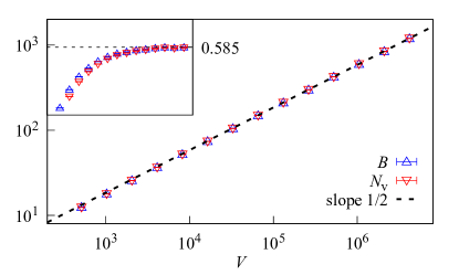
Figure 2: The log-log plot of the bond number $B$ and total number of vertices in the loop clusters $N_{\rm v}$ versus the system volume $V$. The inset displays the rescaled terms $N_{\rm v}/\sqrt{V},B/\sqrt{V}$ versus $V$.

IV Numerical results

IV.1 Scaling behaviors of geometric quantities

In this section, we study the scaling behaviors of some geometric quantities such as the number of bonds $B$ and the number of clusters $N_{\rm k}$, and the sizes of the first- and second-largest clusters $F_{1},F_{2}$ in the loop representation. We perform least-square fits to our data. As a precaution against correction-to-scaling terms that we missed including in the fitting ansatz, we impose a lower cutoff $V\geq V_{\rm min}$ on the data points admitted in the fit and systematically study the effect on the residuals $\chi^{2}$ value by increasing $V_{\rm min}$. In general, the preferred fit for any given ansatz corresponds to the smallest $V_{\rm min}$ for which the goodness of the fit is reasonable and for which subsequent increases in $V_{\rm min}$ do not cause the $\chi^{2}$ value to drop by vastly more than one unit per degree of freedom. In practice, by “reasonable” we mean that $\chi^{2}/\rm{DF}\approx 1$, where DF is the number of degrees of freedom. The systematic error is estimated by comparing estimates from various sensible fitting ansatz.

$\mathcal{O}$	$y_{\mathcal{O}}$	$a_{0}$	$b_{1}$	$y_{1}$	$\chi^{2}/DF$	$V_{\rm min}$
	0.499 9(2)	0.586(2)	-0.68(7)	-0.49(2)	7.1/9	$2^{10}$
	0.499 8(3)	0.587(2)	-0.65(12)	-0.48(3)	7.0/8	$2^{11}$
	0.500 1(3)	0.584(2)	-1.1(4)	-0.55(6)	4.7/7	$2^{12}$
$B$	0.499 98(6)	0.585 6(5)	-0.725(8)	-1/2	7.5/10	$2^{10}$
	0.499 96(8)	0.585 7(6)	-0.728(13)	-1/2	7.4/9	$2^{11}$
	1/2	0.585 3(1)	-0.73(4)	-0.501(7)	7.6/10	$2^{10}$
	1/2	0.585 4(1)	-0.74(6)	-0.503(11)	7.4/9	$2^{11}$
	0.499 8(2)	0.457(1)	0.44(9)	-0.54(4)	7.2/9	$2^{10}$
	0.499 8(2)	0.457(2)	0.5(2)	-0.55(6)	7.1/8	$2^{11}$
$F_{1}$	0.500 2(4)	0.455(3)	0.2(1)	-0.4(1)	5.4/7	$2^{12}$
	0.500 09(7)	0.455 5(3)	0.361(7)	-1/2	8.4/10	$2^{10}$
	0.500 06(8)	0.455 7(4)	0.356(10)	-1/2	7.9/9	$2^{11}$
	0.499 6(2)	0.092 5(2)	1.13(7)	-0.68(1)	9.1/9	$2^{10}$
	0.499 6(2)	0.092 6(3)	1.12(13)	-0.68(2)	9.1/8	$2^{11}$
$F_{2}$	0.499 8(3)	0.092 3(4)	0.9(2)	-0.66(3)	8.5/7	$2^{12}$
	0.499 81(9)	0.092 3(1)	1.023(8)	-2/3	9.7/9	$2^{11}$
	0.499 7(1)	0.092 4(1)	1.01(3)	-2/3	8.6/8	$2^{12}$

Table 1: The fitting results of the bond number $B$, the first- and second-largest clusters $F_{1}$, $F_{2}$. We conjecture all of them have the same scaling behavior $F_{1},F_{2},B\sim\sqrt{V}$, which suggests there is no two-length scaling behavior in the loop representation.

We first consider the number of bonds $B$. In Fig. 2, we plot $B$ versus the system volume $V$ in log-log scale, and the dashed line with slope $1/2$ suggests $B\sim\sqrt{V}$. Meanwhile, the inset plots $B/\sqrt{V}$ showing that its amplitude tends to 0.585. These results are consistent with our theoretical analysis in Eq. (17).

To extract the scaling behaviors of $B$, we perform the least-square fits via the general ansatz:

$$\mathcal{O}=V^{y_{\mathcal{O}}}(a_{0}+b_{1}V^{y_{1}}+b_{2}V^{y_{2}})+c,$$ (20)

where $\mathcal{O}$ corresponds to the quantities measured, such as $B$, and $y_{\mathcal{O}}$ corresponds to the dominant scaling exponent as $y_{\textsc{b}}$ for $B$. For $B$, we first leave all parameters free, which gives unstable results. We then fix $b_{2}=c=0$ and leave $y_{\textsc{b}}$, $a_{0}$, $b_{1}$ and $y_{1}$ free, and it gives reasonable estimate $y_{\textsc{b}}=0.499\,8(3)$ and $y_{1}=-0.48(3)$ for $V_{\rm min}=2^{11}$. We then try to fit by fixing $y_{1}=-1/2$, as predicted in Eq. (17), and the fitting gives a reasonable estimate $y_{\textsc{b}}=0.499\,96(8)$. More trials have been tried, like fixing $b_{1}=b_{2}=0$ and leaving $y_{\textsc{b}}$, $a_{0}$ and $c$ free, which gives consistent results. Including the systematic errors by comparing various reasonable results, we finally obtain the estimates $y_{\textsc{b}}=0.500\,0(8)$ and $a_{0}=0.585(6)$, both of which are consistent with Eq. (17). The fitting details are summarized in Table 1.

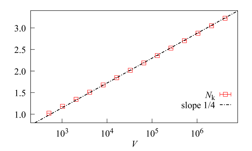
Figure 3: The semi-log plot of the cluster number $N_{\rm k}$ versus $V$, which suggests it scales as $N_{\rm k}\sim\frac{1}{4}\ln V$.

For a given loop configuration, a loop cluster is defined as a set of vertices which are connected together by loop bonds. We next study the geometric properties of these loop clusters. In the graph theory, we have the Euler formula $N_{\rm v}-B=N_{c}-N_{\rm k}$ with the number of cycles $N_{c}$ and the number of clusters $N_{\rm k}$. It inspires us to observe whether the Eulerian clusters in the loop representation are uni-cyclic or multi-cyclic by evaluating $N_{\rm v}$, since for the uni-cyclic graph, $N_{c}$ equals to $N_{\rm k}$. Figure 2 presents the FSS behavior of $N_{\rm v}$ and $N_{\rm v}/\sqrt{V}$ in the inset. It suggests that the value of $N_{\rm v}$ is numerically consistent with $B$ as $V$ is large enough. Therefore, we can argue that $N_{c}=N_{\rm k}$ in thermodynamic limit, which means that all the loop clusters are asymptotically uni-cyclic in the thermodynamic limit.

$\mathcal{O}$	$a$	$b_{1}$	$y_{1}$	$c$	$\chi^{2}/DF$	$V_{\rm min}$
	0.249 8(4)	1.1(2)	-0.49(4)	-0.587(6)	4.7/9	$2^{10}$
$N_{c}$	0.249 6(4)	1.4(6)	-0.53(8)	-0.584(7)	4.4/8	$2^{11}$
	0.249 7(1)	1.17(3)	-1/2	-0.586(2)	4.8/10	$2^{10}$
	0.249 8(2)	1.19(4)	-1/2	-0.587(2)	4.6/9	$2^{11}$

Table 2: The fitting result of the cluster number $N_{\rm k}$, which scales as $N_{\rm k}\sim\ln V$ with the coefficient consistent with 1/4.

Besides, we also study the scaling behavior of the number of loop clusters. As shown in Fig. 3, our data of $N_{\rm k}$ collapse onto the dashed line with slope $1/4$ in semi-log scale, indicating that $N_{\rm k}\sim\frac{1}{4}\ln V$. We can fit the data of $N_{\rm k}$ to the ansatz,

$$N_{\mathcal{O}}=a\ln{V}+b_{1}V^{y_{1}}+b_{2}V^{y_{2}}+c.$$ (21)

We first leave all parameters free, but there is no stable fit. Then by fixing $b_{2}=0$, we obtain stable fits, with details shown in Table 2. We estimate $a=0.249~{}7(5)$ which leads to a conjecture $N_{\rm k}\asymp\frac{1}{4}\ln{V}$.

We then consider the sizes of the largest cluster $F_{1}$ and second-largest cluster $F_{2}$. As Fig. 4 shows, we plot $F_{1}$ and $F_{2}$ in the log-log plot, and the slope $1/2$ indicates both of them have the same scaling behavior $F_{1},F_{2}\sim\sqrt{V}$. In other words, no two-length scaling behavior has been observed, which is different from the observation of two largest clusters in the FK Ising model on the CG Luczak and Łuczak (2006); Fang et al. (2021).

We also perform the least-square fit via (20) for $F_{1}$, $F_{2}$ as $y_{\mathcal{O}}$ corresponds to the volume fractal dimensions $d_{\rm f1}$ and $d_{\rm f2}$, respectively. The fitting results through different trails are reported in Table 1. We obtain the estimates $d_{\rm f1}=0.500\,0(9)$ and $a_{0}=0.456(6)$ for $F_{1}$ while $d_{\rm f2}=0.499\,7(6)$ and $a_{0}=0.092\,4(8)$ for $F_{2}$. We found both $d_{\rm f1}$ and $d_{\rm f2}$ are consistent with $1/2$, and the amplitude $a_{0}$ of $F_{2}$ is much smaller than that of $F_{1}$.

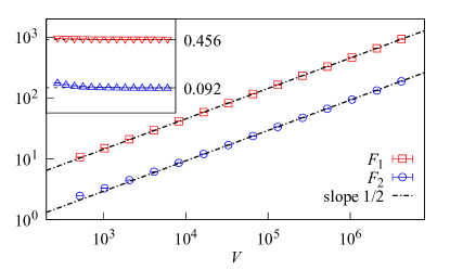
Figure 4: The log-log plot of the size of the largest cluster $F_{1}$, the second-largest cluster $F_{2}$ versus the system volume $V$. Our data suggest $F_{1},F_{2}\sim\sqrt{V}$. The inset displays the rescaled terms $F_{1}/\sqrt{V},F_{2}/\sqrt{V}$ versus $V$.

IV.2 Probability distribution of geometric quantities

Firstly, we investigate the probability distribution of the number of bonds $\mathcal{B}$. Denote $f(\mathcal{B},V)$ the probability density function (PDF) of $\mathcal{B}$ sampled in our simulations. Since $B\sim\sqrt{V}$, we define $X_{B}=\mathcal{B}/\sqrt{V}$ and $f_{X_{B}}(x)$ the PDF of $X_{B}$. Then it follows that

$$f(\mathcal{B},V)d\mathcal{B}=f_{X_{B}}(x)dx,$$ (22)

where $\sqrt{V}dx=d\mathcal{B}$, and thus $f_{X_{B}}(x)=\sqrt{V}f(\mathcal{B},V)$. From Eq. (19), one obtains $f_{X_{B}}(x)=A_{B}\exp(-x^{2}/3)x^{-1/2}$ with $A_{B}=\frac{3^{-1/4}}{2}\Gamma^{-1}(\frac{5}{4})$. Figure 5 presents the distribution of $X_{B}$, and the dashed curve displays $f_{X_{B}}(x)$. It is obvious that our numerical result is consistent with the theoretical analysis. Besides, we found out the probability of the vacant graph (no occupied bond) $P^{\rm v}$ obeys a power-law decay as $V^{-1/4}$, as suggested by the log-log plot of $P^{\rm v}$ versus $V$ in the inset of Fig. 5 and Eq. (19). We perform a least-square fit to the ansatz Eq. (20) and estimate the power-law exponent of $P^{\rm v}$ as $y_{\mathcal{O}}=-0.249(1)$ and the coefficient $a=1.56(3)$.

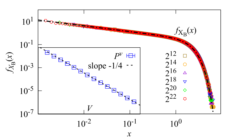
Figure 5: Log-log plot of probability distribution of the number of bonds $\mathcal{B}$ on the CG in the loop representation. Here $f_{X_{B}}(x)$ is the probability density function of $X_{B}=\mathcal{B}/\sqrt{V}$. The solid black line referring to $f_{0}(x)=A_{B}\exp(-x^{2}/3)x^{-1/2}$ verifies that the numerical result is consistent to the theoretical analysis based on the spin representation. The inset shows the probability of vacant graph $P^{\rm v}$ versus $V$ with log-log plot, which implies $P^{\rm v}$ exhibits a power-law decay as $V^{-1/4}$.

Then we study $f_{\mathcal{F}_{1}}(s,V)$, the PDF of $\mathcal{F}_{1}$. Since its mean scales as $\sqrt{V}$, we first study the distribution of $X_{1}:=\mathcal{F}_{1}/\sqrt{V}$. Figure 6 presents the PDF of $f_{X_{1}}(x)$ versus $x$ in the log-log scale. The excellent data collapse suggest that $f_{X_{1}}(x)$ follows a power-law distribution

$$f_{X_{1}}(x)\asymp x^{-1/2}\tilde{f}(x)\;,$$ (23)

with $\tilde{f}(x\to 0)\approx 1/2$ when $x$ is small and $\tilde{f}(x)$ decays quickly to zero when $x$ is large, as indicated from the inset of Figure 6.

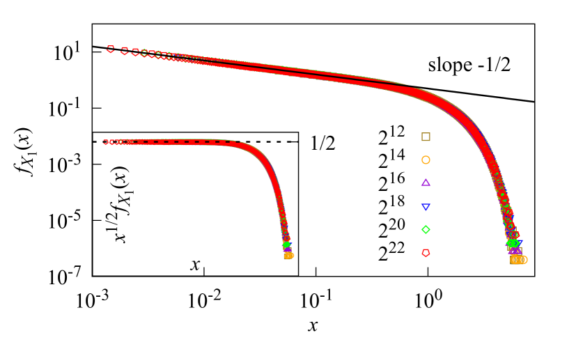
Figure 6: Log-log plot of probability distribution of the largest cluster $\mathcal{F}_{1}$ on the CG in loop representation, where $f_{X_{1}}(x)$ is the probability density function of $X_{1}=\mathcal{F}_{1}/\sqrt{V}$. The inset shows the log-log plot of $f_{X_{1}}(x)x^{1/2}$ versus the rescaled variable $x$.

Meanwhile, we also study the cluster-number density of the loop representation $n(s,V)$. Our results of $n(s,V)$ on the CG, shown in Fig. 7, indicate that it follows the form $n(s,V)\sim s^{-\tau}\tilde{n}(s/V^{d_{F}})$ with a modified Fisher exponent $\tau=1$. More specifically, we can conjecture that the distribution obeys

$$n(s,V)\asymp n_{0}s^{-\tau}V^{-h}\tilde{n}(s/V^{d_{F}})\;,$$ (24)

where $h\geq 0$ is the scaling exponent, $\tilde{n}(x)$ is scaling function which is approximately 1 when $x$ is small. This leads to the number of loop clusters as the integral of $n(s,V)$ from $1$ to the largest loop cluster

$$N_{\rm k}=V\int_{1}^{F_{1}}n(s,V)ds.$$ (25)

Our previous results suggest $F_{1}\sim a_{0}\sqrt{V}$, so it follows that

$$N_{\rm k}\asymp\left\{\begin{array}[]{lr}\frac{n_{0}}{2}V^{1-h}(\ln{V}+\ln{a_{0}})&\rm{if}\ \ \tau=1,\\ \frac{n_{0}}{1-\tau}a_{0}^{1-\tau}V^{1+\frac{1}{2}(1-\tau)-h}&\rm{if}\ \ \tau\neq 1.\end{array}\right.$$ (26)

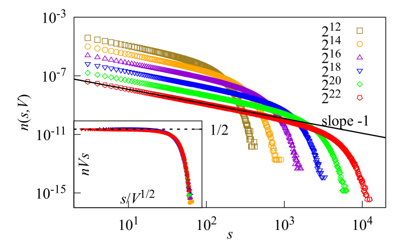
Figure 7: Cluster-number density of the loop representation in the log-log scale. The inset shows the plot of $n(s,V)Vs$ versus $s/\sqrt{V}$, which implies that the scaling function is consistent with $1/2$ when $s/\sqrt{V}\ll 1$.

In the previous section, we know $N_{\rm k}\asymp\frac{\ln{V}}{4}$. Therefore, we obtain $n_{0}=\frac{1}{2},h=1,\tau=1$. The inset of Fig. 7 confirms our conjecture, including $n_{0}=\frac{1}{2}$.

Therefore, in contrast to the FK representation, the scaling behaviors of $f_{{\mathcal{F}}_{1}}(s,V)$ and $n(s,V)$ both show that there is only one scaling sector and one length scale in the loop representation.

IV.3 Insights for the anomalous FSS behaviors in the random-cluster representation

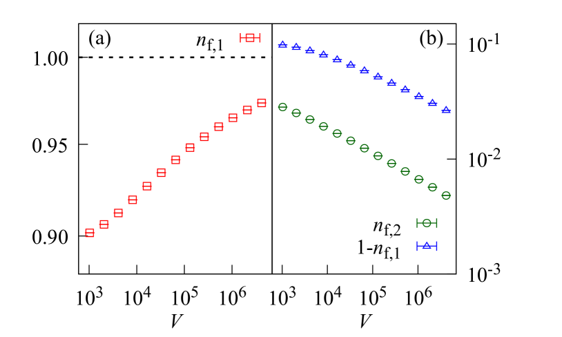
Figure 8: Panel (a) plots the relative loop vertices in the largest FK cluster $n_{\rm f,1}$ versus $V$. Panel (b) shows the log-log plot of the relative loop vertices in the second-largest FK cluster $n_{\rm f,2}$ and the one out of the largest FK cluster $1-n_{\rm f,1}$ versus $V$. It implies that all the loop clusters belong to the largest FK cluster as $V\to\infty$.

As discovered in above sections, the loop bond density $\frac{B}{V}\sim\frac{1}{\sqrt{V}}$, so the loop configuration is vacant in the thermodynamic limit. Moreover, the probability of adding bonds through the LC algorithm is asymptotically the same as the critical percolation threshold $1/V$, such that the transformation from the loop representation to the FK representation is almost the process of critical percolation. In this section, we will demonstrate how LC algorithm can provide an intuitive understanding to the rich critical phenomenon in the FK representation Fang et al. (2022a, b).

Firstly, in the FK representation, the largest and second-largest clusters exhibit distinct scaling behaviors: $C_{1}\sim V^{3/4}$ and $C_{2}\sim\sqrt{V}\log{V}$. However, as Fig. 4 shows, the first- and second-largest clusters in the loop representation both scale as $\sqrt{V}$. One would wonder what happens in the percolation process of the LC algorithm. We record the relative mass of the loop clusters belonging to the first- and second-largest FK clusters after the representation transformation denoted as $n_{\rm f,1},n_{\rm f,2}$. As shown in Fig. 8(a), the relative loop vertices in $\mathcal{C}_{1}$ increases to $1$ as the system volume becomes larger. In contrast, Fig. 8(b) shows that the relative loop vertices in $\mathcal{C}_{2}$ and out of $\mathcal{C}_{1}$ exhibit a power-law decay to zero as $V$ increases. Furthermore, we perform a least-square fit to Eq. (20) for $1-n_{\rm f,1}$, and we obtain the decaying exponent $y_{\textsc{d}}=0.225(6)$. These evidences suggest that in the thermodynamic limit, all loop clusters belong to the largest FK cluster $C_{1}$ after the percolation process while cycles in other FK clusters are newly generated in the process of percolation.

Secondly, two sectors are observed in the configuration space of the FK representation: the percolation sector $S^{\rm P}$ with its size of the largest cluster $\mathcal{C}_{1}\leq O(V^{2/3})$ and the Ising sector $S^{\rm I}$ for otherwise. The percolation sector vanishes with the rate $V^{-1/12}$ and the largest cluster in this sector scales as $C_{1}^{\rm P}\sim V^{2/3}$. We are trying to find out what the percolation sector corresponds to in the loop configuration space.

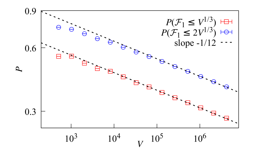
Figure 9: Log-log plot of the probability that the loop configuration in the conjectured percolation sector $P(\mathcal{F}_{1}\leq\alpha V^{1/3})$ with $\alpha=1$ or $2$. The straight dashed black lines with slope $-1/12$ are to guide the eye.

In graph theory, a bridge is a bond whose deletion would break a cluster into two. The configuration with all bridges deleted is called bridge-free configuration. The clusters in the loop representation are all bridge-free clusters. From Ref. Huang et al. (2018), we know that the volume fractal dimension of the bridge-free cluster in the CG-percolation model is $d_{B}=\frac{1}{3}$, so we conjecture that the corresponding percolation sector in the loop representation $S^{\rm P}_{l}$ consists of the configurations whose $\mathcal{F}_{1}\leq\alpha V^{\frac{1}{3}}$ with some constant $\alpha$. The probability of $S^{\rm P}_{l}$ can be derived from the probability distribution of the largest loop cluster $f_{\mathcal{F}_{1}}(s,V)$(23) :

$$P(S^{\rm P}_{l}) =P(\mathcal{F}_{1}\leq\alpha V^{1/3})\approx 2\alpha^{\frac{1}{2}}\tilde{f}(0)V^{-\frac{1}{12}}\;,$$ (27)

which is perfectly consistent with the probability of the percolation sector in the FK representation as $P(S^{\rm P})\sim V^{-1/12}$. The numerical result of $P(\mathcal{F}_{1}\leq\alpha V^{1/3})$ with $\alpha=1,2$ versus $V$ is shown in Fig. 9. We perform a least-square fit to Eq. (20) with our $P(S^{\rm P}_{l})$ data and obtain $y_{\mathcal{O}}=-0.081(2)$ for $\alpha=1$, which is consistent with $-\frac{1}{12}$. By fixing $y_{\mathcal{O}}=-\frac{1}{12}$, we estimate the coefficient $2\alpha^{\frac{1}{2}}\tilde{f}(0)=0.986(4)$ for $\alpha=1$ and $2\alpha^{\frac{1}{2}}\tilde{f}(0)=1.388(4)$ for $\alpha=2$. It then follows that $\tilde{f}(0)=0.48(2)$ which is consistent with our conjecture $1/2$.

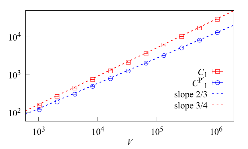
Figure 10: Log-log plot of the largest cluster size of the FK-Ising model $C_{1}$ and the largest cluster size of the configurations generated from the loop configurations where $\mathcal{F}_{1}\leq 2V^{1/3}$, denoted as $C_{1}^{\rm P^{\prime}}$, versus $V$. The red dashed line with slope $2/3$ and the blue dashed line with slope $3/4$ imply the difference between their volume fractal dimensions.

To further verify our conjecture, we observe the scaling behavior of the largest FK cluster generated by performing the percolation process to the loop configurations where $\mathcal{F}_{1}\leq 2V^{1/3}$, denoted as $C^{\rm P^{\prime}}_{1}$. We show the data of $C^{\rm P^{\prime}}_{1}$ and the largest cluster size of the FK Ising model $C_{1}$ in Fig. 10; the former scales as $V^{2/3}$ and the latter scales $V^{3/4}$. This confirms our conjecture that the percolation sector in the FK Ising model corresponds to the loop configurations with the largest loop size of order $V^{1/3}$.

Thirdly, we consider the case away from the critical point and define $t=(K_{c}-K)/K_{c}$. When the critical point is approached from high-temperature side ($t>0$), the magnetic susceptibility $\chi(t,V)=V\langle m^{2}\rangle=V^{2y_{h}-1}\tilde{\chi}(tV^{y_{t}})$ with renormalization-group exponents $(y_{t}=1/2,y_{h}=3/4)$. Based on the FSS assumption, as $x\to\infty$, the scaling function $\tilde{\chi}(x)\sim x^{-\gamma}$ with $\gamma=(2y_{h}-1)/y_{t}=1$, which recovers the thermodynamic scaling behavior $\chi(t)\sim t^{-\gamma}$.

Recall in Sec. III, the bond number $B=\frac{1}{2}V\langle m^{2}\rangle+O(1)=\frac{1}{2}\chi+O(1)$. Thus, one would expect

$$B=\sqrt{V}\tilde{B}(t\sqrt{V}),$$ (28)

where the scaling function $\tilde{B}(x)\sim x^{-1}$ as $x\to\infty$. Then, if one takes $t=O(V^{-1/3})$, one would obtain $B\sim\sqrt{V}\cdot(V^{-1/3+1/2})^{-1}=V^{1/3}$, which is the same as the scaling of the bridge-free bond number for the CG-percolation model Huang et al. (2018). At this temperature, the FK clusters obtained by adding bonds via the LC algorithm are expected to behave the same as CG-percolation clusters, which explains the existence of percolation scaling window in the FK Ising model and the width is of order $O(V^{-1/3})$. While the temperature is decreased from $K_{c}$, the bond number increases and no percolation scaling window is observed.

V Discussion

In this work, we study the geometric properties of the complete-graph (CG) Ising model in the loop representation. Theoretically, we derive that the density of bonds decays as $V^{-1/2}$, which means the loop configurations are basically vacant in the thermodynamic limit. We numerically find that the volume fractal dimension for the first- and second-largest loop clusters is $1/2$, and the number of clusters scales as $\frac{1}{4}\ln{V}$. We also observe that the bond number is numerically consistent with the number of vertices in loop clusters, and this means these loops are uni-cyclic, which is similar to the bridge-free configurations of the CG-percolation model. Based on our numerical results, we conjecture the exact form of the probability distribution of the largest loop cluster and the cluster-number density $n(s,V)$. In Ref. Ben-Naim and Krapivsky (2005), the authors used the rate equation approach to study and derive the cycle-length number density of the critical percolation on the CG, which scales as $(2sV)^{-1}$ with a cutoff at $O(V^{1/3})$. Thus, it has the same behavior as our $n(s,V)$ except the different cutoff.

The abundant critical behaviors in the Fortuin-Kasteleyn (FK) representation, i.e., the emergence of two length scales, two configuration sectors, and two scaling windows, are not found in the loop representation. But, via the loop-cluster (LC) joint model, results in the loop representation does provide a vivid and intuitive understanding to these critical behaviors in the FK representation. Under the LC joint model, the FK representation can be regarded as playing a percolation game on top of loop configurations. During the percolation process, almost all loops are connected together and end up with forming the largest FK cluster. Other FK clusters are basically these newly generated percolation clusters.

It is generally believed that the CG is a mean-field approximation to high-dimensional tori. Recently, the FK Ising model on lattices above the upper critical dimension $d_{c}=4$ was studied and the similar scaling behaviors (two length scales, two sectors and two scaling windows) were again observed Fang et al. (2022a, b). More interestingly, in addition to the well-known upper critical dimension $d_{c}=4$, these anomalous scaling behaviors uncover a new upper critical dimension $d_{p}=6$, which cannot be observed in the spin representation. Therefore, a number of questions naturally arise. First, can the LC joint model provide an understanding to the anomalous behaviors of the FK representation on high-dimensional lattices? Second, can the two-upper-critical-dimensional phenomena be observed in the loop representation? Third, can the loop representation provide a straightforward understanding for the existence of two upper critical dimensions? These open questions will be investigated in our future work.

References

- Duminil-Copin (2022) H. Duminil-Copin, arXiv:2208.00864 (2022).
- Onsager (1944) L. Onsager, Physical Review 65, 117 (1944).
- Aizenman and Fernández (1986) M. Aizenman and R. Fernández, Journal of Statistical Physics 44, 393–454 (1986).
- Aizenman et al. (2015) M. Aizenman, H. Duminil-Copin, and V. Sidoravicius, Communications in Mathematical Physics 334, 719 (2015).
- van der Waerden (1941) B. L. van der Waerden, Zeitschrift für Physik 118, 473 (1941).
- Duminil-Copin (2016) H. Duminil-Copin, arXiv:1607.06933 (2016).
- Grimmett and Janson (2007) G. Grimmett and S. Janson, Random even graphs (2007).
- Wu (1982) F. Y. Wu, Reviews of Modern Physics 54, 235 (1982).
- Fortuin and Kasteleyn (1972) C. M. Fortuin and P. W. Kasteleyn, Physica 57, 536 (1972).
- Grimmett (2006) G. Grimmett, The random-cluster model, Vol. 333 (Springer, 2006).
- Fang et al. (2022a) S. Fang, Z. Zhou, and Y. Deng, Chinese Physics Letters 39, 080502 (2022a).
- Fang et al. (2022b) S. Fang, Z. Zhou, and Y. Deng, arXiv:2212.08544 (2022b).
- Francesco et al. (2012) P. Francesco, P. Mathieu, and D. Sénéchal, Conformal field theory (Springer Science & Business Media, 2012).
- Kager and Nienhuis (2004) W. Kager and B. Nienhuis, Journal of Statistical Physics 115, 1149 (2004).
- Cardy (2005) J. Cardy, Annals of Physics 318, 81 (2005).
- Aizenman and Duminil-Copin (2021) M. Aizenman and H. Duminil-Copin, Annals of Mathematics 194, 163 (2021).
- Swendsen and Wang (1987) R. H. Swendsen and J.-S. Wang, Phys. Rev. Lett. 58, 86 (1987).
- Edwards and Sokal (1988) R. G. Edwards and A. D. Sokal, Phys. Rev. D 38, 2009 (1988).
- Zhang et al. (2020) L. Zhang, M. Michel, E. M. Elçi, and Y. Deng, Phys. Rev. Lett. 125, 200603 (2020).
- Luczak and Łuczak (2006) M. Luczak and T. Łuczak, Random Structures & Algorithms 28, 215 (2006).
- Note (1) Spatial length is not defined on the complete graph. Here the two length (size) scales mean that, compared with the self-similarity property commonly observed in many critical systems, the largest cluster in the FK Ising model is much larger than other clusters.
- Fang et al. (2021) S. Fang, Z. Zhou, and Y. Deng, Phys. Rev. E 103, 012102 (2021).
- Elçi et al. (2018) E. M. Elçi, J. Grimm, L. Ding, A. Nasrawi, T. M. Garoni, and Y. Deng, Phys. Rev. E 97, 042126 (2018).
- Note (2) In this paper, means that while means their ratio converges to some positive constant.
- Note (3) The volume fractal dimension is to characterize how cluster sizes scale with respect to the system volume.
- Huang et al. (2018) W. Huang, P. Hou, J. Wang, R. M. Ziff, and Y. Deng, Phys. Rev. E 97, 022107 (2018).
- Prokof’ev and Svistunov (2001) N. Prokof’ev and B. Svistunov, Phys. Rev. Lett. 87, 160601 (2001).
- Blöte and Deng (2002) H. W. J. Blöte and Y. Deng, Phys. Rev. E 66, 066110 (2002).
- Luijten (1997) E. Luijten, Interaction range, universality and the upper critical dimension (Delft University Press, 1997).
- Ben-Naim and Krapivsky (2005) E. Ben-Naim and P. L. Krapivsky, Physical Review E 71, 026129 (2005).