Identification and Estimation of Categorical Random Coefficient Models

Abstract

This paper proposes a linear categorical random coefficient model, in which the random coefficients follow parametric categorical distributions. The distributional parameters are identified based on a linear recurrence structure of moments of the random coefficients. A Generalized Method of Moments estimation procedure is proposed also employed by Peter Schmidt and his coauthors to address heterogeneity in time effects in panel data models. Using Monte Carlo simulations, we find that moments of the random coefficients can be estimated reasonably accurately, but large samples are required for estimation of the parameters of the underlying categorical distribution. The utility of the proposed estimator is illustrated by estimating the distribution of returns to education in the U.S. by gender and educational levels. We find that rising heterogeneity between educational groups is mainly due to the increasing returns to education for those with postsecondary education, whereas within group heterogeneity has been rising mostly in the case of individuals with high school or less education.

Keywords: Random coefficient models, categorical distribution, return to education

JEL Code: C01, C21, C13, C46, J30

1 Introduction

Random coefficient models have been used extensively in time series, cross-section and panel regressions. Nicholls and Pagan (1985) consider the estimation of first and second moments of the random coefficient $\beta_{i}$ and the error term $u_{i}$, in a linear regression model. In the seminal work, Beran and Hall (1992) establish the conditions of identifying and estimating the distribution of $\beta_{i}$ and $u_{i}$ non-parametrically. The baseline linear univariate regression in Beran and Hall (1992) has been extended in non-parametric framework by Beran (1993); Beran and Millar (1994); Beran, Feuerverger, and Hall (1996); Hoderlein, Klemelä, and Mammen (2010, 2017) and Breunig and Hoderlein (2018), to just name a few. Hsiao and Pesaran (2008) survey random coefficient models in linear panel data models.

In some econometric applications, Hausman (1981); Hausman and Newey (1995); Foster and Hahn (2000) for examples, the main interest is to estimate the consumer surplus distribution based on a linear demand system where the coefficient associated with the price is random. In such settings, the distribution of the random coefficients is needed when computing the consumer surplus function, and the non-parametric estimation is more general, flexible and suitable for the purpose. On the other hand, parametric models may be favored in applications in which the implied economic meaning of the distribution of the random coefficients is of interests. Examples include estimation of the return to education (Lemieux, 2006b, c) and the labor supply equation (Bick, Blandin, and Rogerson, 2022).

In this paper, we consider a linear regression model with a random coefficient $\beta_{i}$ that is assumed to follow a categorical distribution, i.e. $\beta_{i}$ has a discrete support $\left\{b_{1},b_{2},\cdots,b_{K}\right\}$, and $\beta_{i}=b_{k}$ with probability $\pi_{k}$. The discretization of the support of the random coefficient $\beta_{i}$ naturally corresponds to the interpretation that each individual belongs to a certain category, or group, $k$ with probability $\pi_{k}$. Compared to a non-parametric distribution with continuous support, assuming a categorical distribution allows us not only to model the heterogeneous responses across individuals but also to interpret the results with sharper economic meaning. As we will illustrate in the empirical application in Section 6, it is hard to clearly interpret the distribution of returns to education without imposing some form of parametric restrictions.

In addition, with the categorical distribution imposed, the identification and estimation of the distribution of $\beta_{i}$ do not rely on identically distributed error terms $u_{i}$ and regressors $\mathbf{w}_{i}$, as shown in Section 2 and 3. Heterogeneously generated errors can be allowed, which is important in many empirical applications. To the best of our knowledge, this is the first identification result in linear random coefficient model without a strict IID setting.

The identification of the distribution of $\beta_{i}$ is established in this paper based on the identification of the moments of $\beta_{i}$, which coincides with the identification condition in Beran and Hall (1992) that the distribution of $\beta_{i}$ is uniquely determined by its moments, which is assumed to exist up to an arbitrary order. Since under our setup the distribution of $\beta_{i}$ is parametrically specified, the moments of $\beta_{i}$ exist and can be derived explicitly. The parameters of the assumed categorical distribution can then be uniquely determined by a system of equations in terms of the moments, as in Theorem 2. The parameters of the categorical distribution are then estimated consistently by the generalized method of moments (GMM). The estimation procedure based on moment conditions shares similar spirits as in Ahn, Lee, and Schmidt (2001, 2013) in which Peter Schmidt and coauthors study panel data models with interactive effects where they allow for the time effects to vary across individual units. Comparing to alternative non-parametric random coefficient models, the standard GMM estimation is easy to implement, and the identified categorical structure has a clear economic interpretation.

Using Monte Carlo (MC) simulations, we find that moments of the random coefficients can be estimated reasonably accurately, but large samples are required for estimation of the parameters of the underlying categorical distributions. Our theoretical and MC results also suggest that our method is suitable when the number heterogeneous coefficients and the number of categories are small (2 or 3). With the number of categories rising the burden on identification from the moments to the parameters of the categorical distribution also rises rapidly. The quality of identification also deteriorates as we need to rely on higher and higher moments to identify a larger number of categories, since the information content of the moments tend to decline with their order.

The proposed method is also illustrated by providing estimates of the distribution of returns to education in the U.S. by gender and educational levels, using the May and Outgoing Rotation Group (ORG) supplements of the Current Population Survey (CPS) data. Comparing the estimates obtained over the sub-periods 1973-75 and 2001-03, we find that rising between group heterogeneity is largely due to rising returns to education in the case of individuals with postsecondary education, whilst within group heterogeneity has been rising in the case of individuals with high school or less education.

Related Literature: This paper draws mainly upon the literature of random coefficient models. As already mentioned, the main body of the recent literature is focused on non-parametric identification and estimation. Following Beran and Hall (1992), Beran (1993) and Beran and Millar (1994) extend the model to a linear semi-parametric model with a multivariate setup and propose a minimum distance estimator for the unknown distribution. Foster and Hahn (2000) extend the identification results in Beran and Hall (1992) and apply the minimum distance estimator to a gasoline consumption data to estimate the consumer surplus function. Beran, Feuerverger, and Hall (1996) and Hoderlein, Klemelä, and Mammen (2010) propose kernel density estimators based on the Radon inverse transformation in linear models.

In addition to linear models, Ichimura and Thompson (1998) and Gautier and Kitamura (2013) incorporate the random coefficients in binary choice models. Gautier and Hoderlein (2015) and Hoderlein, Holzmann, and Meister (2017) consider triangular models with random coefficients allowing for causal inference. Matzkin (2012) and Masten (2018) discuss the identification of random coefficients in simultaneous equation models. Breunig and Hoderlein (2018) propose a general specification test in a variety of random coefficient models. Random coefficients are also widely studied in panel data models, for example Hsiao and Pesaran (2008) and Arellano and Bonhomme (2012)

The rest of the paper is organized as follows: Section 2 establishes the main identification results. The GMM estimation procedure is proposed and discussed in Section 3. An extension to a multivariate setting is considered in Section 4. Small sample properties of the proposed estimator are investigated in Section 5, using Monte Carlo techniques under different regressor and error distributions. Section 6 presents and discusses our empirical application to the return to education. Section 7 provides some concluding remarks and suggestions for future work. Technical proofs are given in Appendix A.1.

Notations: Largest and smallest eigenvalues of the $p\times p$ matrix $\mathbf{A}=\left(a_{ij}\right)$ are denoted by $\lambda_{\max}\left(\mathbf{A}\right)$ and $\lambda_{\min}\left(\mathbf{A}\right),$ respectively, its spectral norm by $\left\|\mathbf{A}\right\|=\lambda_{\max}^{1/2}\left(\mathbf{A}^{\prime}\mathbf{A}\right)$, $\mathbf{A}\succ 0$ means that $\mathbf{A}$ is positive definite, $\mathrm{vech\left(\mathbf{A}\right)}$ denotes the vectorization of distinct elements of $\mathbf{A}$, $\mathbf{0}$ denotes zero matrix (or vector). For $\mathbf{a}\in\mathbb{R}^{p}$, $\mathrm{diag}\left(\mathbf{a}\right)$ represents the diagonal matrix with elements of $a_{1},a_{2},\cdots,a_{p}$. For random variables (or vectors) $u$ and $v$, $u\perp v$ represents $u$ is independent of $v$. We use $c$ ($C$) to denote some small (large) positive constants. For a differentiable real-valued function $f\left(\mathbf{\theta}\right)$, $\nabla_{\mathbf{\theta}}f\left(\mathbf{\theta}\right)$ denotes the gradient vector. Operator $\rightarrow_{p}$ denotes convergence in probability, and $\rightarrow_{d}$ convergence in distribution. The symbols $O(1)$, and $O_{p}(1)$ denote asymptotically bounded deterministic and random sequences, respectively.

2 Categorical random coefficient model

We suppose the single cross-section observations, $\left\{y_{i},x_{i},\mathbf{z}_{i}\right\}_{i=1}^{n}$, follow the categorical random coefficient model

$$y_{i}=x_{i}\beta_{i}+\mathbf{z}_{i}^{\prime}\mathbf{\gamma}+u_{i},$$ (2.1)

where $y_{i},x_{i}\in\mathbb{R}$, $\mathbf{z}_{i}\in\mathbb{R}^{p_{z}},$ and $\beta_{i}\in\left\{b_{1},b_{2},\cdots,b_{K}\right\}$ admits the following $K$-categorical distribution,

$$\beta_{i}=\begin{cases}b_{1},&\text{w.p. }\pi_{1},\\ b_{2},&\text{w.p. }\pi_{2},\\ \vdots&\vdots\\ b_{K},&\text{w.p. }\pi_{K},\end{cases}$$ (2.2)

w.p. denotes “with probability”, $\pi_{k}\in\left(0,1\right)$, $\sum_{k=1}^{K}\pi_{k}=1$, $b_{1}<b_{2}<\cdots<b_{K}$, $\mathbf{\gamma}\in\mathbb{R}^{p_{z}}$ is homogeneous and $\mathbf{z}_{i}$ could include an intercept term as its first element. It is assumed that $\beta_{i}\perp\mathbf{w}_{i}=\left(x_{i},\mathbf{z}_{i}^{\prime}\right)^{\prime}$, and the idiosyncratic errors $u_{i}$ are independently distributed with mean $0$.

Remark 1

The model can be extended to allow $\mathbf{x}_{i},\mathbf{\beta}_{i}\in\mathbb{R}^{p}$, with $\mathbf{\beta}_{i}$ following a multivariate categorical distribution, though with more complicated notations. We will consider possible extensions in Section 4.

Remark 2

Since we consider a pure cross-sectional setting, the key assumption that $\beta_{i}$ and $x_{i}$ are independently distributed cannot be relaxed. Allowing $\beta_{i}$ to vary with $w_{i}$, without any further restrictions, is tantamount to assuming $y_{i}$ is a general function of $w_{i}$, in effect rendering a nonparametric specification.

Remark 3

The number of categories $K$ is assumed to be fixed and known. Conditions $\sum_{k=1}^{K}\pi_{k}=1$, $b_{1}<b_{2}<\cdots<b_{K},$ and $\pi_{k}\in\left(0,1\right)$ together are sufficient for the existence of $K$ categories. For example, if $b_{k}=b_{k^{\prime}}$, then we can merge categories $k$ and $k^{\prime}$, and the number of categories reduces to $K-1$. Similarly, if $\pi_{k}=0$ for some $k$, then category $k$ can be deleted, and the number of categories is again reduced to $K-1$. Information criteria can be used to determine $K$, but this will not be pursued in this paper. Model specification tests could also be considered. See, for examples, Andrews (2001) and Breunig and Hoderlein (2018).

In the rest of this section, we focus on the model (2.1) and establish the conditions under which the distribution of $\beta_{i}$ is identified.

2.1 Identifying the moments of $\beta_{i}$

Assumption 1

1. (i) $u_{i}$ is distributed independently of $\mathbf{w}_{i}=\left(x_{i},\mathbf{z}_{i}^{\prime}\right)^{\prime}$ and $\beta_{i}$. (ii) $\sup_{i}\mathrm{E}\left(\left|u_{i}^{r}\right|\right)<C$, $r=1,2,\cdots,2K-1$. (iii) $n^{-1}\sum_{i=1}^{n}u_{i}^{4}=O_{p}(1)$.

2. (i) Let $\mathbf{Q}_{n,ww}=n^{-1}\sum_{i=1}^{n}\mathbf{w}_{i}\mathbf{w}_{i}^{\prime}$, and $\mathbf{q}_{n,wy}=n^{-1}\sum_{i=1}^{n}\mathbf{w}_{i}y_{i}$. Then $\left\|\mathrm{E}\left(\mathbf{Q}_{n,ww}\right)\right\|<C<\infty$, and $\left\|\mathrm{E}\left(\mathbf{q}_{n,wy}\right)\right\|<C<\infty$, and there exists $n_{0}\in\mathbb{N}$ such that for all $n\geq n_{0}$,

   $$0<c<\lambda_{\min}\left(\mathbf{Q}_{n,ww}\right)<\lambda_{\max}\left(\mathbf{Q}_{n,ww}\right)<C<\infty.$$

   (ii) $\sup_{i}\mathrm{E}\left(\left\|\mathbf{w}_{i}\right\|^{r}\right)<C<\infty$, $r=1,2,\cdots,4K-2$.
   (iii) $n^{-1}\sum_{i=1}^{n}\left\|\mathbf{w}_{i}\right\|^{4}=O_{p}(1)$.

3. $\left\|\mathbf{Q}_{n,ww}-\mathrm{E}\left(\mathbf{Q}_{n,ww}\right)\right\|=O_{p}\left(n^{-1/2}\right)$, $\left\|\mathbf{q}_{n,wy}-\mathrm{E}\left(\mathbf{q}_{n,wy}\right)\right\|=O_{p}\left(n^{-1/2}\right)$, and

   $$\mathrm{E}\left(\mathbf{Q}_{n,ww}\right)=n^{-1}\sum_{i=1}^{n}\mathrm{E}\left(\mathbf{w}_{i}\mathbf{w}_{i}^{\prime}\right)\succ 0.$$

4. $\left\|\mathrm{E}\left(\mathbf{Q}_{n,ww}\right)-\mathbf{Q}_{ww}\right\|=O\left(n^{-1/2}\right)$, $\left\|\mathrm{E}\left(\mathbf{q}_{n,wy}\right)-\mathbf{q}_{wy}\right\|=O\left(n^{-1/2}\right)$, where $\mathbf{q}_{wy}=\lim\limits_{n\to\infty}\mathrm{E}\left(\mathbf{q}_{n,wy}\right)$, $\mathbf{Q}_{ww}=\lim\limits_{n\to\infty}\mathrm{E}\left(\mathbf{Q}_{n,ww}\right)$ and $\mathbf{Q}_{ww}\succ 0$.

Remark 4

Part (a) of Assumption 1 relaxes the assumption that $u_{i}$ is identically distributed, and allows for heterogeneously generated errors. For identification of the distribution of $\beta_{i}$, we require $u_{i}$ to be distributed independently of $\mathbf{w}_{i}$ and $\beta_{i}$, which rules out conditional heteroskedasticity. However, estimation and inference involving $\mathrm{E}\left(\beta_{i}\right)$ and $\mathbf{\gamma}$ can be carried out in presence of conditionally error heteroskedastic, as shown in Theorem 3. Parts (c) and (d) of Assumption 1 relax the condition that $\mathbf{w}_{i}$ is identically distributed across $i$. As we proceed, only $\beta_{i}$, whose distribution is of interest, is assumed to be IID across $i$, and it is not required for $\mathbf{w}_{i}$ and $u_{i}$ to be identically distributed over $i$.

Remark 5

The high level conditions in Assumption 1, concerning the convergence in probability of averages such as $Q_{n,ww}=n^{-1}\sum_{i=1}^{n}\mathbf{w}_{i}\mathbf{w}_{i}^{\prime}$, can be verified under weak cross-sectional dependence. Let $f_{i}=f\left(\mathbf{w}_{i},\beta_{i},u_{i}\right)$ be a generic function of $\mathbf{w}_{i}$, $\beta_{i}$ and $u_{i}$. Assume that $\sup_{i}\mathrm{E}\left(f_{i}^{2}\right)<C$, and $\sup_{j}\sum_{i=1}^{n}\left|\mathrm{cov}\left(f_{i},f_{j}\right)\right|<C$, for some fixed $C<\infty$. Then,

$$\mathrm{var}\left(\frac{1}{n}\sum_{i=1}^{n}f_{i}\right)\leq\frac{1}{n^{2}}\sum_{i=1}^{n}\sum_{j=1}^{n}\left|\mathrm{cov}\left(f_{i},f_{j}\right)\right|\leq\frac{1}{n}\sup_{j}\sum_{i=1}^{n}\left|\mathrm{cov}\left(f_{i},f_{j}\right)\right|\leq\frac{C}{n}.$$

By Chebyshev’s inequality, for any $\varepsilon>0$, we have $M_{\varepsilon}>\sqrt{C/\varepsilon}$ such that

$$\Pr\left(\sqrt{n}\left|\frac{1}{n}\sum_{i=1}^{n}\left[f_{i}-\mathrm{E}\left(f_{i}\right)\right]\right|>M_{\varepsilon}\right)\leq\frac{n\mathrm{var}\left(n^{-1}\sum_{i=1}^{n}f_{i}\right)}{C}\varepsilon\leq\varepsilon,$$

i.e. $n^{-1}\sum_{i=1}^{n}\left[f_{i}-\mathrm{E}\left(f_{i}\right)\right]=O_{p}\left(n^{-1/2}\right)$.

Denote $\mathbf{\phi}_{i}=\left(\beta_{i},\mathbf{\gamma}^{\prime}\right)^{\prime}$ and $\mathbf{\phi}=\mathrm{E}\left(\mathbf{\phi}_{i}\right)=\left(\mathrm{E}\left(\beta_{i}\right),\mathbf{\gamma}^{\prime}\right)^{\prime}$. Consider the moment condition,

$$\mathrm{E}\left(\mathbf{w}_{i}y_{i}\right)=\mathrm{E}\left(\mathbf{w}_{i}\mathbf{w}_{i}^{\prime}\right)\mathbf{\phi},$$ (2.3)

and sum (2.3) over $i$

$$\frac{1}{n}\sum_{i=1}^{n}\mathrm{E}\left(\mathbf{w}_{i}y_{i}\right)=\left[\frac{1}{n}\sum_{i=1}^{n}\mathrm{E}\left(\mathbf{w}_{i}\mathbf{w}_{i}^{\prime}\right)\right]\mathbf{\phi}.$$ (2.4)

Let $n\to\infty$, then $\mathbf{\phi}$ is identified by

$$\mathbf{\phi}=\mathbf{Q}_{ww}^{-1}\mathbf{q}_{wy},$$ (2.5)

under Assumption 1.

Assumption 2

Let $\tilde{y}_{i}=y_{i}-\mathbf{z}_{i}^{\prime}\mathbf{\gamma}$.

1. $\left|n^{-1}\sum_{i=1}^{n}\mathrm{E}\left(\tilde{y}_{i}^{r}x_{i}^{s}\right)-\rho_{r,s}\right|=O\left(n^{-1/2}\right),$ and $\left|\rho_{r,s}\right|<\infty,$ for $r,s=0,1,\cdots,2K-1$.

2. $\left|n^{-1}\sum_{i=1}^{n}\mathrm{E}\left(u_{i}^{r}\right)-\sigma_{r}\right|=O\left(n^{-1/2}\right),$ and $\left|\sigma_{r}\right|<\infty$, for $r=2,3,\cdots,2K-1$.

3. $n^{-1}\sum_{i=1}^{n}\left[\mathrm{var}(x_{i}^{r})-\left(\rho_{0,2r}-\rho_{0,r}^{2}\right)\right]=O\left(n^{-1/2}\right)$ where $\rho_{0,2r}-\rho_{0,r}^{2}>0,$ for $r=2,3,\cdots,2K-1$.

Remark 6

The above assumption allows for a limited degree of heterogeneity of the moments. As an example, let $\mathrm{E}\left(u_{i}^{r}\right)=\sigma_{ir}$ and denote the heterogeneity of the $r^{th}$ moment of $u_{i}$ by $e_{ir}=\sigma_{ir}-\sigma_{r}$. Then

$$\left|n^{-1}\sum_{i=1}^{n}\mathrm{E}\left(u_{i}^{r}\right)-\sigma_{r}\right|\leq n^{-1}\sum_{i=1}^{n}\left|e_{ir}\right|,$$

and condition (b) of Assumption 2 is met if $\ \sum_{i=1}^{n}\left|e_{ir}\right|=O(n^{\alpha_{r}})$ with $\alpha_{r}<1/2$. $\alpha_{r}$ measures the degree of heterogeneity with $\alpha_{r}=1$ representing the highest degree of heterogeneity. A similar idea is used by Pesaran and Zhou (2018) in their analysis of poolability in panel data models.

Theorem 1

Under Assumptions 1 and 2, $\mathrm{E}\left(\beta_{i}^{r}\right)$ and $\sigma_{r}$, $r=2,3,\cdots,2K-1$ are identified.

Proof. For $r=2,\cdots,2K-1$,

$$\mathrm{E}\left(\tilde{y}_{i}^{r}\right) =\mathrm{E}\left(x_{i}^{r}\right)\mathrm{E}\left(\beta_{i}^{r}\right)+\mathrm{E}\left(u_{i}^{r}\right)+\sum_{q=2}^{r-1}\binom{r}{q}\mathrm{E}\left(x_{i}^{r-q}\right)\mathrm{E}\left(u_{i}^{q}\right)\mathrm{E}\left(\beta_{i}^{r-q}\right),$$ (2.6)

$$\mathrm{E}\left(\tilde{y}_{i}^{r}x_{i}^{r}\right) =\mathrm{E}\left(x_{i}^{2r}\right)\mathrm{E}\left(\beta_{i}^{r}\right)+\mathrm{E}\left(x_{i}^{r}\right)\mathrm{E}\left(u_{i}^{r}\right)+\sum_{q=2}^{r-1}\binom{r}{q}\mathrm{E}\left(x_{i}^{2r-q}\right)\mathrm{E}\left(u_{i}^{q}\right)\mathrm{E}\left(\beta_{i}^{r-q}\right).$$ (2.7)

where $\binom{r}{q}=\frac{r!}{q!(r-q)!}$ are binomial coefficients, for non-negative integers $q\leq r$.

Sum over $i$, then by parts (a) and (b) of Assumption 2,

$$\rho_{0,r}\mathrm{E}\left(\beta_{i}^{r}\right)+\sigma_{r} =\rho_{r,0}-\sum_{q=2}^{r-1}\binom{r}{q}\rho_{0,r-q}\sigma_{q}\mathrm{E}\left(\beta_{i}^{r-q}\right),$$ (2.8)

$$\rho_{0,2r}\mathrm{E}\left(\beta_{i}^{r}\right)+\rho_{0,r}\sigma_{r} =\rho_{r,r}-\sum_{q=2}^{r-1}\binom{r}{q}\rho_{0,2r-q}\sigma_{q}\mathrm{E}\left(\beta_{i}^{r-q}\right).$$ (2.9)

Derivation details are relegated to Appendix A.1. By part (c) of Assumption 2, the matrix $\begin{pmatrix}\rho_{0,r}&1\\ \rho_{0,2r}&\rho_{0,r}\end{pmatrix}$ is invertible for $r=2,3,\cdots,2K-1$. As a result, we can sequentially solve (2.8) and (2.9) for $\mathrm{E}\left(\beta_{i}^{r}\right)$ and $\sigma_{r}$, for $r=2,3,\cdots,2K-1$.   

2.2 Identifying the distribution of $\beta_{i}$

Beran and Hall (1992, Theorem 2.1, pp. 1972) prove the identification of the distribution of the random coefficient, $\beta_{i}$, in a canonical model without covariates, $z_{i}$, under the condition that the distribution of $\beta_{i}$ is uniquely determined by its moments. We show the identification of moments of $\beta_{i}$ holds more generally when $x_{i}$ and $u_{i}$ are not identically distributed and the distribution of $\beta_{i}$ is identified if it follows a categorical distribution. Note that under (2.2),

$$\mathrm{E}\left(\beta_{i}^{r}\right)=\sum_{k=1}^{K}\pi_{k}b_{k}^{r},\;r=0,1,2,\cdots,2K-1,$$ (2.10)

with $\mathrm{E}\left(\beta_{i}^{r}\right)$ identified under Assumption 1. To identify $\mathbf{\pi}=\left(\pi_{1},\pi_{2},...,\pi_{K}\right)^{\prime}$ and $\mathbf{b}=\left(b_{1},b_{2},...,b_{K}\right)^{\prime}$, we need to verify that the system of $2K$ equations in (2.10) has a unique solution if $b_{1}<b_{2}<\cdots<b_{K}$, and $\pi_{k}\in\left(0,1\right)$. In the proof, we construct a linear recurrence relation and make use of the corresponding characteristic polynomial.

Theorem 2

Consider the random coefficient regression model (2.1), suppose that Assumptions 1 and 2 hold. Then $\mathbf{\theta}=\left(\mathbf{\pi}^{\prime},\mathbf{b}^{\prime}\right)^{\prime}$ is identified subject to $b_{1}<b_{2}<\cdots<b_{K}$ and $\pi_{k}\in\left(0,1\right)$, for all $k=1,2,\cdots,K$.

Proof. We motivate the key idea of the proof in the special case where $K=2,$ and relegate the proof of the general case to the Appendix A.1. Let $b_{1}=\beta_{L}$, $b_{2}=\beta_{H}$, $\pi_{1}=\pi$ and $\pi_{2}=1-\pi$. Note that

$$\mathrm{E}\left(\beta_{i}\right) =\pi\beta_{L}+\left(1-\pi\right)\beta_{H},$$ (2.11)

$$\mathrm{E}\left(\beta_{i}^{2}\right) =\pi\beta_{L}^{2}+\left(1-\pi\right)\beta_{H}^{2},$$ (2.12)

$$\mathrm{E}\left(\beta_{i}^{3}\right) =\pi\beta_{L}^{3}+\left(1-\pi\right)\beta_{H}^{3},$$ (2.13)

and $\mathrm{E}\left(\beta_{i}^{k}\right)$, $k=1,2,3$ are identified. $\left(\pi,\beta_{L},\beta_{H}\right)$ can be identified if the system of equations (2.11) to (2.13), has a unique solution. By (2.11),

$$\pi=\frac{\beta_{H}-\mathrm{E}\left(\beta_{i}\right)}{\beta_{H}-\beta_{L}},\;\text{and}\;1-\pi=\frac{\mathrm{E}\left(\beta_{i}\right)-\beta_{L}}{\beta_{H}-\beta_{L}}.$$ (2.14)

Plug (2.14) into (2.12) and (2.13),

$$\mathrm{E}\left(\beta_{i}\right)\left(\beta_{L}+\beta_{H}\right)-\beta_{L}\beta_{H} =\mathrm{E}\left(\beta_{i}^{2}\right),$$ (2.15)

$$\mathrm{E}\left(\beta_{i}^{2}\right)\left(\beta_{L}+\beta_{H}\right)-\mathrm{E}\left(\beta_{i}\right)\beta_{L}\beta_{H} =\mathrm{E}\left(\beta_{i}^{3}\right).$$ (2.16)

Denote $\beta_{L+H}=\beta_{L}+\beta_{H}$ and $\beta_{LH}=\beta_{L}\beta_{H}$, and write (2.15) and (2.16) in matrix form,

$$\mathbf{M}\mathbf{D}\mathbf{b}^{\ast}=\mathbf{m},$$ (2.17)

where

$$\mathbf{M}=\begin{pmatrix}1&\mathrm{E}\left(\beta_{i}\right)\\ \mathrm{E}\left(\beta_{i}\right)&\mathrm{E}\left(\beta_{i}^{2}\right)\end{pmatrix},\,\mathbf{D}=\begin{pmatrix}-1&0\\ 0&1\end{pmatrix},\,\mathbf{b}^{\ast}=\begin{pmatrix}\beta_{LH}\\ \beta_{L+H}\end{pmatrix},\;\text{and}\;\mathbf{m}=\begin{pmatrix}\mathrm{E}\left(\beta_{i}^{2}\right)\\ \mathrm{E}\left(\beta_{i}^{3}\right)\end{pmatrix}.$$

Under the conditions $0<\pi<1$ and $\beta_{H}>\beta_{L}$,

$$\det\left(\mathbf{M}\right)=\mathrm{var}\left(\beta_{i}\right)=\mathrm{E}\left(\beta_{i}^{2}\right)-\mathrm{E}\left(\beta_{i}\right)^{2}=\pi\left(1-\pi\right)\left(\beta_{H}-\beta_{L}\right)^{2}>0.$$

As a result, we can solve (2.17) for $\beta_{L+H}$ and $\beta_{LH}$ as

$$\beta_{L+H} =\frac{\mathrm{E}\left(\beta_{i}^{3}\right)-\mathrm{E}\left(\beta_{i}\right)\mathrm{E}\left(\beta_{i}^{2}\right)}{\mathrm{var}\left(\beta_{i}\right)},$$ (2.18)

$$\beta_{LH} =\frac{\mathrm{E}\left(\beta_{i}\right)\mathrm{E}\left(\beta_{i}^{3}\right)-\mathrm{E}\left(\beta_{i}^{2}\right)^{2}}{\mathrm{var}\left(\beta_{i}\right)}.$$ (2.19)

$\beta_{L}$ and $\beta_{H}$ are solutions to the quadratic equation,

$$\beta^{2}-\beta_{L+H}\beta+\beta_{LH}=0.$$ (2.20)

We can verify that $\Delta=\beta_{L+H}^{2}-4\beta_{LH}>0$ by direct calculation using (2.18) and (2.19). Simplifying $\Delta$ in terms of $\mathrm{E}\left(\beta_{i}^{k}\right)$ and then plugging in (2.11), (2.12) and (2.13),

$$\Delta= \frac{\left[\mathrm{E}\left(\beta_{i}^{3}\right)-\mathrm{E}\left(\beta_{i}\right)\mathrm{E}\left(\beta_{i}^{2}\right)\right]^{2}-4\mathrm{var}\left(\beta_{i}\right)\left[\mathrm{E}\left(\beta_{i}\right)\mathrm{E}\left(\beta_{i}^{3}\right)-\mathrm{E}\left(\beta_{i}^{2}\right)^{2}\right]}{\left[\mathrm{var}\left(\beta_{i}\right)\right]^{2}}$$

$$=\left(\beta_{H}-\beta_{L}\right)^{2}>0.$$

Then, we obtain the unique solutions,

$$\beta_{L} =\frac{1}{2}\left(\beta_{L+H}-\sqrt{\beta_{L+H}^{2}-4\beta_{LH}}\right),$$ (2.21)

$$\beta_{H} =\frac{1}{2}\left(\beta_{L+H}+\sqrt{\beta_{L+H}^{2}-4\beta_{LH}}\right),$$ (2.22)

and $\pi$ can be determined by (2.14) correspondingly.   

Remark 7

The key identifying assumption in (2) is the assumed existence of the strict ordinal relation $b_{1}<b_{2}<\cdots<b_{K}$ so that $b_{k}$ and $b_{k^{\prime}}$ are not symmetric for $k\neq k^{\prime}$, and $0<\pi_{k}<1$ so that the distribution of $\beta_{i}$ does not degenerate. When $K=2$, the conditions $b_{1}<b_{2}<\cdots<b_{K}$, and $\pi_{k}\in\left(0,1\right)$, are equivalent to $\mathrm{var}\left(\beta_{i}\right)=\pi_{1}\left(1-\pi_{1}\right)\left(b_{2}-b_{1}\right)^{2}>0$. In other words, not surprisingly, the categorical distribution of $\beta_{i}$ are identified only if $\mathrm{var}\left(\beta_{i}\right)>0$.

In practice, a test for $\mathbb{H}_{0}:\mathrm{var}\left(\beta_{i}\right)=0$ is possible, by noting that $\mathrm{var}\left(\beta_{i}\right)=0$ is equivalent to

$$\kappa^{2}=\frac{\mathrm{E}\left(\beta_{i}\right)^{2}}{\mathrm{E}\left(\beta_{i}^{2}\right)}=1,$$

where $\kappa^{2}$ is well-defined as long as $\beta_{i}\not\equiv 0$. One important advantage of basing the test of slope homogeneity on $\kappa^{2}$ rather than on $var(\beta_{i})=0$, is that $\kappa^{2}\,$is scale-invariant. $\mathrm{E}\left(\beta_{i}\right)$ and $\mathrm{E}\left(\beta_{i}^{2}\right)$ are identified as in Section 2.1, whose consistent estimation does not require $\mathrm{var}\left(\beta_{i}\right)>0$. Consequently, in principle it is possible to test slope homogeneity by testing $\mathbb{H}_{0}:\kappa^{2}=1$. However, the problem becomes much more complicated when there are more than two categories and/or there are more than one regressor under consideration. A full treatment of testing slope homogeneity in such general settings is beyond the scope of the present paper.

Remark 8

Note that in the special case of the proof of Theorem 2 where $K=2$, $\beta_{L+H}=\beta_{L}+\beta_{H}$ and $\beta_{LH}=\beta_{L}\beta_{H}$ corresponds to the $b_{1}^{\ast}$ and $b_{2}^{\ast}$ and (2.17) is the same as (A.1.6) when $K=2$. The special case illustrates the procedure of identification: identify $\left(b_{k}^{\ast}\right)_{k=1}^{K}$ by the moments of $\beta_{i}$, then solve for $\left(b_{k}\right)_{k=1}^{K}$ and finally identify $\left(\pi_{k}\right)_{k=1}^{K}$.

3 Estimation

In this section, we propose a generalized method of moments estimator for the distributional parameters of $\beta_{i}$. To reduce the complexity of the moment equations, we first obtain a $\sqrt{n}$-consistent estimator of $\gamma$ and consider the estimation of the distribution of $\beta_{i}$ by replacing $\gamma$ by $\hat{\gamma}$.

3.1 Estimation of $\gamma$

Let $\mathbf{\phi}=\left(\mathrm{E}\left(\beta_{i}\right),\mathbf{\gamma}^{\prime}\right)^{\prime}$, $v_{i}=\beta_{i}-\mathrm{E}\left(\beta_{i}\right)$ and using the notation in Assumption 1, (2.1) can be written as

$$y_{i}=\mathbf{w}_{i}^{\prime}\mathbf{\phi}+\xi_{i},$$ (3.1)

where $\xi_{i}=u_{i}+x_{i}v_{i}$. Then $\mathbf{\phi}$ can be estimated consistently by $\hat{\mathbf{\phi}}=\mathbf{Q}_{n,ww}^{-1}\mathbf{q}_{n,wy}$ where $\mathbf{Q}_{n,ww}$ and $\mathbf{q}_{n,wy}$ are defined in Assumption 1.

Assumption 3

$\left\|n^{-1}\sum_{i=1}^{n}\mathrm{E}\left(\mathbf{w}_{i}\mathbf{w}_{i}^{\prime}\xi_{i}^{2}\right)-\mathbf{V}_{w\xi}\right\|=O\left(n^{-1/2}\right)$, $\mathbf{V}_{w\xi}\succ 0,$ and

$$\left\|\frac{1}{n}\sum_{i=1}^{n}\mathbf{w}_{i}\mathbf{w}_{i}^{\prime}\xi_{i}^{2}-\frac{1}{n}\sum_{i=1}^{n}\mathrm{E}\left(\mathbf{w}_{i}\mathbf{w}_{i}^{\prime}\xi_{i}^{2}\right)\right\|=O_{p}\left(n^{-1/2}\right).$$ (3.2)

Remark 9

As in the case of Assumption 1, the high level condition (3.2) can be shown to hold under weak cross-sectional dependence, assuming that elements of $\mathbf{w}_{i}\mathbf{w}_{i}^{\prime}\xi_{i}^{2}$ are cross-sectionally weakly correlated over $i$. See Remark 5.

Theorem 3

Under Assumption 1, $\hat{\mathbf{\phi}}$ is a consistent estimator for $\mathbf{\phi}$. In addition, under Assumptions 1 and 3, as $n\to\infty$,

$$\sqrt{n}\left(\hat{\mathbf{\phi}}-\mathbf{\phi}\right)\rightarrow_{d}N\left(\mathbf{0},\mathbf{V}_{\phi}\right),$$ (3.3)

where $\mathbf{V}_{\phi}=\mathbf{Q}_{ww}^{-1}\mathbf{V}_{w\xi}\mathbf{Q}_{ww}^{-1}.$ $\mathbf{V}_{\phi}$ is consistently estimated by

$$\hat{\mathbf{V}}_{\phi}=\mathbf{Q}_{n,ww}^{-1}\hat{\mathbf{V}}_{w\xi}\mathbf{Q}_{n,ww}^{-1}\to_{p}\mathbf{V}_{\phi},$$

as $n\to\infty$, where $\hat{\mathbf{V}}_{w\xi}=n^{-1}\sum_{i=1}^{n}\mathbf{w}_{i}\mathbf{w}_{i}^{\prime}\hat{\xi}_{i}^{2}$, and $\hat{\xi}_{i}=y_{i}-\mathbf{w}_{i}^{\prime}\hat{\mathbf{\phi}}$.

The proof of Theorem 3 is provided in Section S.2 in the online supplement.

3.2 Estimation of the distribution of $\beta_{i}$

Denote the moments of $\beta_{i}$ on the right-hand side of (2.10) by

$$\mathbf{m}_{\beta}=(m_{1},m_{2},...,m_{2K-1})^{\prime}=\left[\mathrm{E}\left(\beta_{i}^{r}\right)\right]_{r=1}^{2K-1}\in\Theta_{m}\subset\left\{\mathbf{m}_{\beta}\in\mathbb{R}^{2K-1}:m_{r}\geq 0,\text{ }r\text{ is even}\right\},$$

and note that

$$\mathbf{m}_{\beta}=\left(\begin{array}[]{c}m_{1}\\ m_{2}\\ \vdots\\ m_{2K-1}\end{array}\right)=\left(\begin{array}[]{cccc}b_{1}&b_{2}&\cdots&b_{K}\\ b_{1}^{2}&b_{2}^{2}&\cdots&b_{K}^{2}\\ \vdots&\vdots&\vdots&\vdots\\ b_{1}^{2K-1}&b_{2}^{2K-1}&\cdots&b_{K}^{2K-1}\end{array}\right)\left(\begin{array}[]{c}\pi_{1}\\ \pi_{2}\\ \vdots\\ \pi_{K}\end{array}\right),$$ (3.4)

so in general we can write $\mathbf{m}_{\beta}\triangleq h\left(\mathbf{\theta}\right),$ where $\mathbf{\theta}=\left(\mathbf{\pi}^{\prime},\mathbf{b}^{\prime}\right)^{\prime}\in\Theta$, and $\mathbf{\theta}$ can be uniquely determined in terms of $\mathbf{m}_{\beta}$ by Theorem 2. To estimate $\mathbf{\theta}$, we consider moment conditions following a similar procedure as in Section 2, and propose a generalized method of moments (GMM) estimator.

We consider the following moment conditions

$$\mathrm{E}\left(\tilde{y}_{i}^{r}\right)=\sum_{q=0}^{r}\binom{r}{q}\mathrm{E}\left(x_{i}^{r-q}\right)\mathrm{E}\left(u_{i}^{q}\right)m_{r-q},\text{ }$$

and

$$\mathrm{E}\left(\tilde{y}_{i}^{r}x_{i}^{s_{r}}\right)=\sum_{q=0}^{r}\binom{r}{q}\mathrm{E}\left(x_{i}^{r-q+s_{r}}\right)\mathrm{E}\left(u_{i}^{q}\right)m_{r-q},$$ (3.5)

where $\mathrm{E}\left(u_{i}\right)=0$, $\tilde{y}_{i}=y_{i}-\mathbf{z}_{i}^{\prime}\mathbf{\gamma}$, $r=1,2,...,2K-1$, and $s_{r}=0,1,\cdots,S-r$, where $S$ is a user-specific tuning parameter, chosen such that the highest order moments of $x_{i}$ included is at most $S$, where $S>2K-1$.

Let $\sigma_{0}=1$ and $\sigma_{1}=0$ such that $\sigma_{r}$ is well-defined for $r=0,1,\cdots,2K-1$. Sum (3.5) over $i$ and rearrange terms,

$$0 =\sum_{q=0}^{r}\binom{r}{q}\left[\frac{1}{n}\sum_{i=1}^{n}\mathrm{E}\left(x_{i}^{r-q+s_{r}}\right)\mathrm{E}\left(u_{i}^{q}\right)\right]m_{r-q}-\frac{1}{n}\sum_{i=1}^{n}\mathrm{E}\left(\tilde{y}_{i}^{r}x_{i}^{s_{r}}\right)$$

$$=\sum_{q=0}^{r}\binom{r}{q}\left[\frac{1}{n}\sum_{i=1}^{n}\mathrm{E}\left(x_{i}^{r-q+s_{r}}\right)\right]\sigma_{q}m_{r-q}-\frac{1}{n}\sum_{i=1}^{n}\mathrm{E}\left(\tilde{y}_{i}^{r}x_{i}^{s_{r}}\right)+\delta_{n}^{(r,s_{r})},$$ (3.6)

where

$$\delta_{n}^{(r,s_{r})}=\sum_{q=0}^{r}\binom{r}{q}\left[\frac{1}{n}\sum_{i=1}^{n}\mathrm{E}\left(x_{i}^{r-q+s_{r}}\right)\left[\mathrm{E}\left(u_{i}^{q}\right)-\sigma_{q}\right]\right]m_{r-q}=O\left(n^{-1/2}\right),$$

as shown in the proof of Theorem 1.

Taking $n\to\infty$ in (3.6),

$$\sum_{q=0}^{r}\binom{r}{q}\rho_{0,r-q+s_{r}}\sigma_{q}m_{r-q}-\rho_{r,s_{r}}=0,$$ (3.7)

by Assumption 2. We stack the left-hand side of (3.7) over $r=1,2,...,2K-1$, and $s_{r}=0,1,\cdots,S-r$ and transform $\mathbf{m}_{\beta}=h\left(\mathbf{\theta}\right)$ to get $\mathbf{g}_{0}\left(\mathbf{\theta},\mathbf{\sigma},\mathbf{\gamma}\right)$.

To implement the GMM estimation we replace $\tilde{y}_{i}$, by $\hat{\tilde{y}}_{i}=y_{i}-\mathbf{z}_{i}^{\prime}\hat{\mathbf{\gamma}}$, and $\rho_{r,s_{r}}$ by $n^{-1}\sum_{i=1}^{n}\hat{\tilde{y}}_{i}^{r}x_{i}^{s_{r}}$. Noting that $\mathbf{m}_{\beta}=h\left(\mathbf{\theta}\right)$, denote the sample version of the left-hand side of (3.7) by

$$\hat{g}_{n}^{(r,s_{r})}\left(\mathbf{\theta},\mathbf{\sigma},\hat{\mathbf{\gamma}}\right)=\frac{1}{n}\sum_{i=1}^{n}\hat{g}_{i}^{(r,s_{r})}\left(\mathbf{\theta},\mathbf{\sigma},\hat{\mathbf{\gamma}}\right),$$ (3.8)

where

$$\hat{g}_{i}^{\left(r,s_{r}\right)}\left(\mathbf{\theta},\mathbf{\sigma},\hat{\mathbf{\gamma}}\right)=\sum_{q=0}^{r}\binom{r}{q}x_{i}^{r-q+s_{r}}\sigma_{q}\left[h\left(\mathbf{\theta}\right)\right]_{r-q}-\hat{\tilde{y}}_{i}^{r}x_{i}^{s_{r}},$$

and $\mathbf{\sigma}=\left(\sigma_{2},\sigma_{3},\cdots,\sigma_{2K-1}\right)^{\prime}$. Stack the equations in (3.8), over $r=0,1,...,2K-1$ and $s_{r}=0,1,\cdots,S-r$ ($S>2K-1$), in vector notations we have

$$\mathbf{\hat{g}}_{n}\left(\mathbf{\theta},\mathbf{\sigma},\hat{\mathbf{\gamma}}\right)=\frac{1}{n}\sum_{i=1}^{n}\mathbf{\hat{g}}_{i}\left(\mathbf{\theta},\mathbf{\sigma},\hat{\mathbf{\gamma}}\right).$$ (3.9)

Given $\hat{\mathbf{\gamma}}$, the GMM estimator of $\left(\mathbf{\theta}^{\prime},\mathbf{\sigma}^{\prime}\right)^{\prime}$ is now computed as

$$\left(\hat{\mathbf{\theta}}^{\prime},\hat{\mathbf{\sigma}}^{\prime}\right)^{\prime}=\arg\min_{\mathbf{\theta}\in\Theta,\mathbf{\sigma}\in\mathcal{S}}\hat{\Phi}_{n}\left(\mathbf{\theta},\mathbf{\sigma},\hat{\mathbf{\gamma}}\right),$$

where $\hat{\Phi}_{n}=\mathbf{\hat{g}}_{n}\left(\mathbf{\theta},\mathbf{\sigma},\hat{\mathbf{\gamma}}\right)^{\prime}\mathbf{A}_{n}\mathbf{\hat{g}}_{n}\left(\mathbf{\theta},\mathbf{\sigma},\hat{\mathbf{\gamma}}\right)$, and $\mathbf{A}_{n}$ is a positive definite matrix. We follow the GMM literature using the following choice of $\mathbf{A}_{n}$,

$$\mathbf{\hat{A}}_{n}=\left[\frac{1}{n}\sum_{i=1}^{n}\mathbf{\hat{g}}_{i}\left(\tilde{\mathbf{\theta}},\tilde{\mathbf{\sigma}},\hat{\mathbf{\gamma}}\right)\mathbf{\hat{g}}_{i}\left(\tilde{\mathbf{\theta}},\tilde{\mathbf{\sigma}},\hat{\mathbf{\gamma}}\right)^{\prime}-\mathbf{\bar{g}}_{n}\mathbf{\bar{g}}_{n}^{\prime}\right]^{-1},$$ (3.10)

where $\mathbf{\bar{g}}_{n}=\frac{1}{n}\sum_{i=1}^{n}\mathbf{\hat{g}}_{i}\left(\tilde{\mathbf{\theta}},\tilde{\mathbf{\sigma}},\hat{\mathbf{\gamma}}\right)$, and $\tilde{\mathbf{\theta}}$ and $\tilde{\mathbf{\sigma}}$ are preliminary estimators.

Assumption 4

Denote the true values of $\mathbf{\theta}$, $\mathbf{\sigma}$ and $\mathbf{\gamma}$ by $\mathbf{\theta}_{0}$, $\mathbf{\sigma}_{0}$ and $\mathbf{\gamma}_{0}$.

1. $\Theta$ and $\mathcal{S}$ are compact. $\mathbf{\theta}_{0}\in\mathrm{int}\left(\Theta\right)$ and $\mathbf{\sigma}_{0}\in\mathrm{int}\left(\mathcal{S}\right)$.

2. $\mathbf{A}_{n}\rightarrow_{p}\mathbf{A}$ as $n\rightarrow\infty$, where $\mathbf{A}$ is some positive definite matrix.

3.  

   $$\frac{1}{n}\sum_{i=1}^{n}\left[\hat{\tilde{y}}_{i}^{r}x_{i}^{s_{r}}-\mathrm{E}\left(\tilde{y}_{i}^{r}x_{i}^{s_{r}}\right)\right]=O_{p}\left(n^{-1/2}\right),$$

   for $r=0,1,2,\cdots,2K-1$, $s_{r}=0,1,\cdots,S-r,$ and $S>2K-1.$

Remark 10

Parts (a) and (b) of Assumption 4 are standard regularity conditions in the GMM literature. Part (c) together with Assumption 2 are high-level regularity conditions which allow us to generalize the usual IID assumption and nest the IID data generation process as a special case. The sample analogue terms in (c) include $\hat{\tilde{y}}_{i}=y_{i}-\mathbf{z}_{i}^{\prime}\hat{\mathbf{\gamma}}$, instead of the infeasible $\tilde{y}_{i}=y_{i}-\mathbf{z}_{i}^{\prime}\mathbf{\gamma}$. The $\sqrt{n}$-consistency of $\hat{\mathbf{\gamma}}$ shown in Theorem 3 ensures that replacing $\tilde{y}_{i}$ by $\hat{\tilde{y}}_{i}$ does not alter the convergence rate.

Theorem 4

Let $\mathbf{\eta}=\left(\mathbf{\theta}^{\prime},\mathbf{\sigma}^{\prime}\right)^{\prime}$ and $\mathbf{\eta}_{0}=\left(\mathbf{\theta}_{0}^{\prime},\mathbf{\sigma}_{0}^{\prime}\right)^{\prime}$. Under Assumptions 1, 2, and 4, $\hat{\mathbf{\eta}}\rightarrow_{p}\mathbf{\eta}_{0}$ as $n\rightarrow\infty$.

The proof of Theorem 4 is provided in Appendix A.1.

Assumption 5

Follow the notations as in Assumption 4 and in addition denote $\mathbf{G}\left(\mathbf{\theta},\mathbf{\sigma},\mathbf{\gamma}\right)=\nabla_{\left(\mathbf{\theta}^{\prime},\mathbf{\sigma}^{\prime}\right)^{\prime}}\mathbf{g}_{0}\left(\mathbf{\theta},\mathbf{\sigma},\mathbf{\gamma}\right)$, $\mathbf{G}_{0}=\mathbf{G}\left(\mathbf{\theta}_{0},\mathbf{\sigma}_{0},\mathbf{\gamma}_{0}\right)$, $\mathbf{G}_{\gamma}\left(\mathbf{\theta},\mathbf{\sigma},\mathbf{\gamma}\right)=\nabla_{\mathbf{\gamma}}\mathbf{g}_{0}\left(\mathbf{\theta},\mathbf{\sigma},\mathbf{\gamma}\right)$, $\mathbf{G}_{0,\gamma}=\mathbf{G}_{\gamma}\left(\mathbf{\theta}_{0},\mathbf{\sigma}_{0},\mathbf{\gamma}_{0}\right)$.

1. $\sqrt{n}\mathbf{\hat{g}}_{n}\left(\mathbf{\theta}_{0},\mathbf{\sigma}_{0},\mathbf{\gamma}_{0}\right)\rightarrow_{d}\mathbf{\zeta}\sim N\left(0,\mathbf{V}\right)$ as $n\to\infty$.

2. $\mathbf{G}_{0}^{\prime}\mathbf{AG}_{0}\succ 0$.

Remark 11

In Assumption 5, parts (a) is the high level condition required to ensure the asymptotic normality of $\mathbf{\hat{g}}_{n}\left(\mathbf{\theta}_{0},\mathbf{\sigma}_{0},\mathbf{\gamma}_{0}\right)$, which can be verified by Lindeberg central limit theorem under low-level regularity conditions. Part (c) of Assumption 5 represents the full-rank condition on $\mathbf{G}_{0}$, required for identification of $\mathbf{\theta}_{0}$ and $\mathbf{\sigma}_{0}$.

By Theorem 3, we have $\sqrt{n}\left(\hat{\mathbf{\gamma}}-\mathbf{\gamma}\right)\rightarrow_{d}\zeta_{\gamma}\sim N(0,V_{\gamma})$. The following theorem shows the asymptotic normality of the GMM estimator $\hat{\mathbf{\eta}}$.

Theorem 5

Under Assumptions 1, 3, 4 and 5,

$$\sqrt{n}\left(\hat{\mathbf{\eta}}-\mathbf{\eta}_{0}\right)\rightarrow_{d}\left(\mathbf{G}_{0}^{\prime}\mathbf{A}\mathbf{G}_{0}\right)^{-1}\mathbf{G}_{0}^{\prime}\mathbf{A}\left(\mathbf{\zeta}+\mathbf{G}_{0,\gamma}\mathbf{\zeta}_{\gamma}\right),$$

as $n\rightarrow\infty$.

The proof of Theorem 5 is provided in Appendix A.1.

Remark 12

In practice, we estimate the variance of the asymptotic distribution of $\hat{\eta}$ by

$$\hat{\mathbf{V}}_{\eta}=\left(\hat{\mathbf{G}}^{\prime}\hat{\mathbf{A}}_{n}\hat{\mathbf{G}}\right)^{-1}\hat{\mathbf{G}}^{\prime}\hat{\mathbf{A}}_{n}\hat{\mathbf{V}}_{\zeta}\hat{\mathbf{A}}_{n}^{\prime}\hat{\mathbf{G}}\left(\hat{\mathbf{G}}^{\prime}\hat{\mathbf{A}}_{n}\hat{\mathbf{G}}\right)^{-1},$$ (3.11)

where $\hat{\mathbf{G}}=\nabla_{\left(\mathbf{\sigma}^{\prime},\mathbf{\theta}^{\prime}\right)^{\prime}}\hat{\mathbf{g}}_{n}\left(\hat{\mathbf{\theta}},\hat{\mathbf{\sigma}},\hat{\gamma}\right)$, $\hat{\mathbf{A}}_{n}$ is given by (3.10), and

$$\hat{\mathbf{V}}_{\zeta}=\frac{1}{n}\sum_{i=1}^{n}\mathbf{\psi}_{n,i}\mathbf{\psi}_{n,i}^{\prime},$$

where

$$\mathbf{\psi}_{n,i}=\hat{\mathbf{g}}_{i}\left(\hat{\mathbf{\theta}},\hat{\mathbf{\sigma}},\hat{\gamma}\right)+\nabla_{\mathbf{\gamma}}\hat{\mathbf{g}}_{n}\left(\hat{\mathbf{\theta}},\hat{\mathbf{\sigma}},\hat{\gamma}\right)\mathbf{L}\mathbf{Q}_{n,ww}^{-1}\left(\mathbf{w}_{i}\hat{\xi}_{i}\right),$$

and $\mathbf{L}=\begin{pmatrix}\mathbf{0}_{p_{z}\times 1}&\mathbf{I}_{p_{z}}\end{pmatrix}$ is the loading matrix that selects $\mathbf{\gamma}$ out of $\mathbf{\phi}$.

4 Multiple regressors with random coefficients

One important extension of the regression model (2.1) is to allow for multiple regressors with random coefficients having categorical distribution. With this in mind consider

$$y_{i}=\mathbf{x}_{i}^{\prime}\mathbf{\beta}_{i}+\mathbf{z}_{i}^{\prime}\mathbf{\gamma}+u_{i},$$ (4.1)

where the $p\times 1$ vector of random coefficients, $\mathbf{\beta}_{i}\in\mathbb{R}^{p}$ follows the multivariate distribution

$$\mathrm{Pr}\left(\beta_{i1}=b_{1k_{1}},\beta_{i2}=b_{2k_{2}},\cdots,\beta_{ip}=b_{pk_{p}}\right)=\pi_{k_{1},k_{2},\cdots,k_{p}},$$ (4.2)

with $k_{j}\in\left\{1,2,\cdots,K\right\}$, $b_{j1}<b_{j2}<\cdots<b_{jK}$, and

$$\sum_{k_{1},k_{2},\cdots,k_{p}\in\left\{1,2,\cdots,K\right\}}\pi_{k_{1},k_{2},\cdots,k_{p}}=1.$$

As in Section 2, $\mathbf{\gamma}\in\mathbb{R}^{p_{z}}$, $\mathbf{w}_{i}=\left(\mathbf{x}_{i}^{\prime},\mathbf{z}_{i}^{\prime}\right)^{\prime}$, $\mathbf{\beta}_{i}\perp\mathbf{w}_{i}$, $u_{i}\perp\mathbf{w}_{i}$, and $u_{i}$ are independently distributed over $i$ with mean $0.$

Example 1 Consider the simple case with $p=2$ and $K=2$. For $j=1,2$, denote two categories as $\left\{L,H\right\}$. The probabilities of four possible combinations of realized $\mathbf{\beta}_{i}$ is summarized in Table 1, where $\pi_{LL}+\pi_{LH}+\pi_{HL}+\pi_{HH}=1$.

Table 1: Distribution of $\mathbf{\beta}_{i}$ with $p=2$ and $K=2$

	$k_{2}=L$	$k_{2}=H$
$k_{1}=L$	$\pi_{LL}=\Pr\left(\beta_{i1}=b_{1L},\beta_{i2}=b_{2L}\right)$	$\pi_{LH}=\Pr\left(\beta_{i1}=b_{1L},\beta_{i2}=b_{2H}\right)$
$k_{1}=H$	$\pi_{HL}=\Pr\left(\beta_{i1}=b_{1H},\beta_{i2}=b_{2L}\right)$	$\pi_{HH}=\Pr\left(\beta_{i1}=b_{1H},\beta_{i2}=b_{2H}\right)$

We first identify the moments of $\mathbf{\beta}_{i}$. As in Section 2, $\mathbf{\phi}=\left(\mathrm{E}\left(\mathbf{\beta}_{i}\right)^{\prime},\mathbf{\gamma}^{\prime}\right)^{\prime}$ is identified by

$$\mathbf{\phi}=\mathbf{Q}_{ww}^{-1}\mathbf{q}_{wy},$$ (4.3)

under Assumption 1. We now consider the identification of the higher order moments of $\mathbf{\beta}_{i}$ up to the finite order $2K-1$.

Since $\mathbf{\gamma}$ is identified as in (4.3), we treat it as known and let $\tilde{y}_{i}^{r}=y_{i}-\mathbf{z}_{i}^{\prime}\mathbf{\gamma}$. For $r=2,3,\cdots,2K-1$, consider the moment conditions

$$\mathrm{E}\left(\tilde{y}_{i}^{r}\right) =\mathrm{E}\left[\left(\mathbf{x}_{i}^{\prime}\mathbf{\beta}_{i}+u_{i}\right)^{r}\right]$$

$$=\mathrm{E}\left[\left(\mathbf{x}_{i}^{\prime}\mathbf{\beta}_{i}\right)^{r}\right]+\mathrm{E}\left(u_{i}^{r}\right)+\sum_{s=2}^{r-1}\binom{r}{s}\mathrm{E}\left[\left(\mathbf{x}_{i}^{\prime}\mathbf{\beta}_{i}\right)^{r-s}\right]\mathrm{E}\left(u_{i}^{s}\right).$$ (4.4)

Note that $\mathbf{x}_{i}^{\prime}\mathbf{\beta}_{i}=\sum_{j=1}^{p}\beta_{ij}x_{ij}$, and

$$\mathrm{E}\left[\left(\sum_{j=1}^{p}\beta_{ij}x_{ij}\right)^{r}\right]=\sum_{\sum_{j=1}^{p}q_{j}=r}\binom{r}{\mathbf{q}}\mathrm{E}\left(\prod_{j=1}^{p}x_{ij}^{q_{j}}\right)\mathrm{E}\left(\prod_{j=1}^{p}\beta_{ij}^{q_{j}}\right),$$

where $\binom{r}{\mathbf{q}}=\frac{r!}{q_{1}!q_{2}!\cdots q_{p}!}$, for non-negative integers $r$, $q_{1}$, $\cdots$, $q_{p}$ with $r=\sum_{j=1}^{p}q_{j}$, denotes the multinomial coefficients. We stack $\prod_{j=1}^{p}x_{ij}^{q_{j}}$ with $\mathbf{q}\in\left\{\mathbf{q}\in\left\{0,1,\cdots r\right\}^{p}:\sum_{j=1}^{p}q_{j}=r\right\}$ in a vector form by denoting

$$\mathbf{\tau}_{r}\left(\mathbf{x}_{i}\right)=\left[\varphi\left(\mathbf{x}_{i},\mathbf{q}_{1}\right),\varphi\left(\mathbf{x}_{i},\mathbf{q}_{2}\right),\cdots,\varphi\left(\mathbf{x}_{i},\mathbf{q}_{\nu_{r}}\right)\right]^{\prime},$$

where $\varphi\left(\mathbf{x}_{i},\mathbf{q}\right)=\prod_{j=1}^{p}x_{ij}^{q_{j}}$ and $\nu_{r}=\binom{r+p-1}{p-1}$ is the number of distinct monomials of degree $r$ on the variables $x_{i1},x_{i2},\cdots,x_{ip}$. Similarly,

$$\mathbf{\tau}_{r}\left(\mathbf{\beta}_{i}\right)=\left[\varphi\left(\mathbf{\beta}_{i},\mathbf{q}_{1}\right),\varphi\left(\mathbf{\beta}_{i},\mathbf{q}_{2}\right),\cdots,\varphi\left(\mathbf{\beta}_{i},\mathbf{q}_{\nu_{r}}\right)\right]^{\prime},$$

where $\varphi\left(\mathbf{\beta}_{i},\mathbf{q}\right)=\prod_{j=1}^{p}\beta_{ij}^{q_{j}}$.

Example 2 Consider $p=2$ and $r=2$, we have

$$\mathbf{\tau}_{2}\left(\mathbf{x}_{i}\right) =\left(x_{i1}^{2},x_{i1}x_{i2},x_{i2}^{2}\right)^{\prime},$$

$$\mathbf{\tau}_{2}\left(\mathbf{\beta}_{i}\right) =\left(\beta_{i1}^{2},\beta_{i1}\beta_{i2},\beta_{i2}^{2}\right)^{\prime},$$

and

$$\mathrm{E}\left[\left(x_{i1}\beta_{i1}+x_{i2}\beta_{i2}\right)^{2}\right] =\mathrm{E}\left(x_{i1}^{2}\right)\mathrm{E}\left(\beta_{i1}^{2}\right)+2\mathrm{E}\left(x_{i1}x_{i2}\right)\mathrm{E}\left(\beta_{i1}\beta_{i2}\right)+\mathrm{E}\left(x_{i2}^{2}\right)\mathrm{E}\left(\beta_{i2}^{2}\right)$$

$$=\left[\mathrm{E}\left(x_{i1}^{2}\right),\mathrm{E}\left(x_{i1}x_{i2}\right),\mathrm{E}\left(x_{i2}^{2}\right)\right]\mathrm{diag}\left[\left(1,2,1\right)^{\prime}\right]\left[\mathrm{E}\left(\beta_{i1}^{2}\right),\mathrm{E}\left(\beta_{i1}\beta_{i2}\right),\mathrm{E}\left(\beta_{i2}^{2}\right)\right]^{\prime}$$

$$=\mathrm{E}\left[\mathbf{\tau}_{2}\left(\mathbf{x}_{i}\right)\right]^{\prime}\mathbf{\Lambda}_{2}\mathrm{E}\left[\mathbf{\tau}_{2}\left(\mathbf{\beta}_{i}\right)\right],$$

where $\mathbf{\Lambda}_{2}=\mathrm{diag}\left[\left(1,2,1\right)^{\prime}\right]$.

Then the moment condition (4.4) can be written as

$$\mathrm{E}\left(\tilde{y}_{i}^{r}\right) =\mathrm{E}\left[\mathbf{\tau}_{r}\left(\mathbf{x}_{i}\right)\right]^{\prime}\mathbf{\Lambda}_{r}\mathrm{E}\left[\mathbf{\tau}_{r}\left(\mathbf{\beta}_{i}\right)\right]+\mathrm{E}\left(u_{i}^{r}\right)$$

$$\quad\quad\quad+\sum_{s=2}^{r-1}\binom{r}{s}\mathrm{E}\left[\mathbf{\tau}_{r-s}\left(\mathbf{x}_{i}\right)\right]^{\prime}\mathbf{\Lambda}_{r-s}\mathrm{E}\left[\mathbf{\tau}_{r-s}\left(\mathbf{\beta}_{i}\right)\right]\mathrm{E}\left(u_{i}^{s}\right),$$ (4.5)

where $\mathbf{\Lambda}_{r}=\mathrm{diag}\left[\left[\binom{r}{\mathbf{q}}\right]_{\sum_{j=1}^{p}q_{j}=r}\right]$ is the $\nu_{r}\times\nu_{r}$ diagonal matrix of multinomial coefficients. We further consider the moment conditions

$$\mathrm{E}\left(\tilde{y}_{i}^{r}\mathbf{\tau}_{r}\left(\mathbf{x}_{i}\right)\right) =\mathrm{E}\left[\mathbf{\tau}_{r}\left(\mathbf{x}_{i}\right)\mathbf{\tau}_{r}\left(\mathbf{x}_{i}\right)^{\prime}\right]\mathbf{\Lambda}_{r}\mathrm{E}\left[\mathbf{\tau}_{r}\left(\mathbf{\beta}_{i}\right)\right]+\mathrm{E}\left[\mathbf{\tau}_{r}\left(\mathbf{x}_{i}\right)\right]\mathrm{E}\left(u_{i}^{r}\right)$$

$$\quad\quad\quad+\sum_{s=2}^{r-1}\binom{r}{s}\mathrm{E}\left[\mathbf{\tau}_{r}\left(\mathbf{x}_{i}\right)\mathbf{\tau}_{r-s}\left(\mathbf{x}_{i}\right)^{\prime}\right]\mathbf{\Lambda}_{r-s}\mathrm{E}\left[\mathbf{\tau}_{r-s}\left(\mathbf{\beta}_{i}\right)\right]\mathrm{E}\left(u_{i}^{s}\right),$$ (4.6)

$r=2,3,\cdots,2K-1$. (4.5) and (4.6) reduce to (2.6) and (2.7) when $p=1$.

Assumption 6

 

1. $\left\|n^{-1}\sum_{i=1}^{n}\mathrm{E}\left(\tilde{y}_{i}^{r}\mathbf{\tau}_{s}\left(\mathbf{x}_{i}\right)\right)-\mathbf{\rho}_{r,s}\right\|=O\left(n^{-1/2}\right),$ and $\left\|\mathbf{\rho}_{r,s}\right\|<\infty$, $r,s=0,1,\cdots,2K-1$.

2. $\left\|n^{-1}\sum_{i=1}^{n}\mathrm{E}\left[\mathbf{\tau}_{r}\left(\mathbf{x}_{i}\right)\mathbf{\tau}_{s}\left(\mathbf{x}_{i}\right)^{\prime}\right]-\mathbf{\Xi}_{r,s}\right\|=O\left(n^{-1/2}\right),$ and $\left\|\mathbf{\Xi}_{r,s}\right\|<\infty$, $r,s=0,1,\cdots,2K-1$.

3. $\left|n^{-1}\sum_{i=1}^{n}\mathrm{E}\left(u_{i}^{r}\right)-\sigma_{r}\right|=O\left(n^{-1/2}\right),$ and $\left|\sigma_{r}\right|<\infty$ for $r=2,3,\cdots,2K-1$.

4. $\left\|n^{-1}\sum_{i=1}^{n}\left[\mathrm{var}\left(\mathbf{\tau}_{r}\left(\mathbf{x_{i}}\right)\right)-\left(\mathbf{\Xi}_{r,r}-\mathbf{\rho}_{0,r}\mathbf{\rho}_{0,r}^{\prime}\right)\right]\right\|=O(n^{-1/2})$, where $\mathbf{\Xi}_{r,r}-\mathbf{\rho}_{0,r}\mathbf{\rho}_{0,r}^{\prime}\succ 0$ for $r=2,3\cdots,2K-1$.

Theorem 6

For any $\mathbf{q}\in\left\{\mathbf{q}\in\left\{0,1,\cdots r\right\}^{p}:\sum_{j=1}^{p}q_{j}=r\right\}$ and $r=2,3,\cdots,2K-1$, $\mathrm{E}\left(\prod_{j=1}^{p}\beta_{ij}^{q_{j}}\right)$ and $\sigma_{r}$ are identified under Assumptions 1 and 6.

Proof. For $r=2,3,\cdots,2K-1$, sum (4.5) and (4.6) over $i,$ go through the same steps as in the proof of Theorem 1, then by Assumptions 6(a) to (c), we have (for $n\rightarrow\infty$)

$$\mathbf{\rho}_{r,0}^{\prime}\mathbf{\Lambda}_{r}\mathrm{E}\left[\mathbf{\tau}_{r}\left(\mathbf{\beta}_{i}\right)\right]+\sigma_{r} =\mathbf{\rho}_{r,0}-\sum_{s=2}^{r-1}\binom{r}{s}\mathbf{\rho}_{0,r-s}\mathbf{\Lambda}_{r-s}\mathrm{E}\left[\mathbf{\tau}_{r-s}\left(\mathbf{\beta}_{i}\right)\right]\sigma_{s},$$ (4.7)

$$\mathbf{\Xi}_{r,r}\mathbf{\Lambda}_{r}\mathrm{E}\left[\mathbf{\tau}_{r}\left(\mathbf{\beta}_{i}\right)\right]+\mathbf{\rho}_{0,r}\sigma_{r} =\mathbf{\rho}_{r,r}-\sum_{s=2}^{r-1}\binom{r}{s}\mathbf{\Xi}_{r,r-s}\mathbf{\Lambda}_{r-s}\mathrm{E}\left[\mathbf{\tau}_{r-s}\left(\mathbf{\beta}_{i}\right)\right]\sigma_{s}.$$ (4.8)

Note that

$$\mathbf{M}_{r}=\begin{pmatrix}\mathbf{\Xi}_{r,r}&\mathbf{\rho}_{0,r}\\ \mathbf{\rho}_{0,r}^{\prime}&1\end{pmatrix}\begin{pmatrix}\mathbf{\Lambda}_{r}&\mathbf{0}\\ \mathbf{0}&1\end{pmatrix},$$

is invertible since $\det\left(\mathbf{M}_{r}\right)=\det\left(\mathbf{\Xi}_{r,r}-\mathbf{\rho}_{0,r}\mathbf{\rho}_{0,r}^{\prime}\right)\det\left(\mathbf{\Lambda}_{r}\right)>0,$ for $r=2,3,\cdots,R$, by Assumption 6(d). As a result, we can sequentially solve (4.7) and (4.8) for $\mathrm{E}\left[\mathbf{\tau}_{r}\left(\mathbf{\beta}_{i}\right)\right]$ and $\sigma_{r}$, for $r=2,3,\cdots,2K-1$.   

We now move from the moments of $\mathbf{\beta}_{i}$ to the distribution of $\mathbf{\beta}_{i}$. We first focus on the identification of the marginal probabilities obtained from (4.2) by averaging out the effects of the other coefficients except for $\beta_{ij}$, namely we initially focus on identification of $\lambda_{jk}=\Pr\left(\beta_{ij}=b_{jk}\right)$, for $k=1,2,\cdots,K,$ and $j=1,2,\cdots,p$.

Remark 13

Focusing on the marginal distribution of $\beta_{i}$ is similar to focusing on estimation of partial derivatives in the context of non-parametric estimation, where the curse of dimensionality applies. Consider the estimation of regressing $y_{i}$ on $\mathbf{x}_{i}=\left(x_{i1},x_{i2},\cdots,x_{ip}\right)^{\prime}$,

$$y_{i}=F\left(x_{i1},x_{i2},\cdots.x_{ip}\right)+u_{i}.$$

Then if $F\left(x_{1},x_{i2},\cdots,x_{ip}\right)$ is a homogeneous function (of degree $1/\mu$), then

$$y_{i}=\sum_{j=1}^{p}\left(\mu\frac{\partial F\left(\cdot\right)}{\partial x_{ij}}\right)x_{ij}+u_{i},$$

and under certain conditions we can treat $\mu\frac{\partial F\left(\cdot\right)}{\partial x_{ij}}\equiv\beta_{ij}$.

By Theorem 6, $\mathrm{E}\left(\beta_{ij}^{r}\right)$ is identified for $r=1,2,\cdots,2K-1$ under Assumptions 1 and 6. By (4.2), we have equations

$$\mathrm{E}\left(\beta_{ij}^{r}\right)=\sum_{k=1}^{K}\lambda_{jk}b_{jk}^{r},$$ (4.9)

$r=0,1,\cdots,2K-1$, which is of the same form as (2.10) and (3.4). To identify $\mathbf{\lambda}_{j}=\left(\lambda_{j1},\lambda_{j2},\cdots,\lambda_{jK}\right)^{\prime}$ and $\mathbf{b}_{j}=\left(b_{j1},b_{j2},\cdots,b_{jK}\right)^{\prime}$, we can verify the system of $2K$ equations in (4.9) has a unique solution if $b_{j1}<b_{j2}<\cdots<b_{jK}$ and $\lambda_{jk}\in\left(0,1\right)$. The following corollary is a direct application of Theorem 2.

Corollary 7

Consider the model (4.1) and suppose that Assumptions 1 and 6 hold. Then the parameters $\mathbf{\theta}_{j}=\left(\mathbf{\lambda}_{j}^{\prime},\mathbf{b}_{j}^{\prime}\right)^{\prime}$ of the marginal distribution of $\beta_{i}$ with respect to $\beta_{ij}$ is identified subject to $b_{j1}<b_{j2}<\cdots<b_{jK}$ and $\lambda_{jk}\in\left(0,1\right)$ for $j=1,2,\cdots,p$.

The problem of identification and estimation of the joint distribution of $\mathbf{\beta}_{i}$ is subject to the curse of dimensionality. We have $K^{p}-1$ probability weights, $\pi_{k_{1},k_{2},\cdots,k_{p}}$, to be identified in addition to the $pK$ categorical coefficients $b_{ij}$ that are identified by Corollary 7. The number of parameters increases rapidly with $p$. Even in the simplest case with $K=2$, the total number of unknown parameters is $2p+2^{p}-1$, which grows exponentially.

Note that the marginal probabilities $\lambda_{jk}$ are related to the joint distribution by

$$\lambda_{jk}=\sum_{k_{1},\cdots,k_{j-1},k_{j+1},\cdots,k_{p}\in\left\{1,2,\cdots,K\right\}}\pi_{k_{1},k_{2},\cdots,k_{j-1},k,k_{j+1},\cdots,k_{p}},$$ (4.10)

$k=1,2,\cdots,K$ and $j=1,2,\cdots,p$. The number of linearly independent equations in (4.10) is $pK-(p-1)$.

Example 3  Consider the same setup as in Example 1 with $p=2$ and $K=2$. The marginal probabilities are obtained by

$$\lambda_{1L}=\Pr\left(\beta_{i1}=b_{1L}\right)=\pi_{LL}+\pi_{LH}, \quad\lambda_{1H}=\Pr\left(\beta_{i1}=b_{1H}\right)=1-\lambda_{1L}=\pi_{HL}+\pi_{HH},$$

$$\lambda_{2L}=\Pr\left(\beta_{i2}=b_{2L}\right)=\pi_{LL}+\pi_{HL}, \quad\lambda_{2H}=\Pr\left(\beta_{i2}=b_{2H}\right)=1-\lambda_{2L}=\pi_{LH}+\pi_{HH}.$$ (4.11)

Note that any equation in (4.11) can be expressed as a linear combination of other three equations, for example $\lambda_{2H}=\lambda_{1L}+\lambda_{1H}-\lambda_{2L}$.

The equations corresponding to the cross-moments, $\mathrm{E}\left(\prod_{j=1}^{p}\beta_{ij}^{q_{j}}\right)$, are

$$\mathrm{E}\left(\prod_{j=1}^{p}\beta_{ij}^{q_{j}}\right)=\sum_{k_{1},k_{2},\cdots,k_{p}\in\left\{1,2,\cdots,K\right\}}\left(\prod_{j=1}^{p}b_{jk_{j}}^{q_{j}}\right)\pi_{k_{1},k_{2},\cdots,k_{p}},$$ (4.12)

for $\mathbf{q}\in\left\{\mathbf{q}\in\left\{0,1,\cdots r-1\right\}^{p}:\sum_{j=1}^{p}q_{j}=r\right\}$, $r=2,\cdots,2K-1$. The linear system (4.12) has

$$\sum_{r=1}^{2K-1}\binom{r+p-1}{p-1}-p(2K-1)$$

equations. Then the total number of equations in (4.10) and (4.12) that can be utilized to identify joint probabilities is $C_{r}=\sum_{r=1}^{2K-1}\binom{r+p-1}{p-1}-pK$, which is smaller than the number of joint probabilities $K^{p}-1$ for large $p$. When $K=2$, $C_{r}<K^{p}-1$ for $p\geq 7$.

Identification and estimation of the joint distribution of $\mathbf{\beta}_{i}$ in the general setting will not be pursued in this paper due to the curse of dimensionality. Instead, we consider special cases, that are empirically relevant, in which identification of the joint distribution of $\mathbf{\beta}_{i}$ can be readily established. We first consider small $p$ and $K$, in particular $p=2$ and $K=2$ as in Example 1.

Example 4 Consider the same setup as in Example 1 with $p=2$ and $K=2$. In addition to (4.11), consider the cross-moment,

$$\mathrm{E}\left(\beta_{i1}\beta_{i2}\right)=b_{1L}b_{2L}\pi_{LL}+b_{1L}b_{2H}\pi_{LH}+b_{1H}b_{2L}\pi_{HL}+b_{1H}b_{2H}\pi_{HH}.$$ (4.13)

Writing (4.11) and (4.13) in matrix form, we have

$$\mathbf{B}\mathbf{\pi}=\mathbf{\lambda},$$

where

$$\mathbf{B}=\begin{pmatrix}1&1&0&0\\ 0&0&1&1\\ 1&0&1&0\\ b_{1L}b_{2L}&b_{1L}b_{2H}&b_{1H}b_{2L}&b_{1H}b_{2H}\end{pmatrix},\,\mathbf{\pi}=\begin{pmatrix}\pi_{LL}\\ \pi_{LH}\\ \pi_{HL}\\ \pi_{HH}\end{pmatrix},\,\mathbf{\lambda}=\begin{pmatrix}\lambda_{1L}\\ \lambda_{1H}\\ \lambda_{2L}\\ \mathrm{E}\left(\beta_{i1}\beta_{i2}\right)\end{pmatrix}.$$

Note that $\mathrm{E}\left(\beta_{i1}\beta_{i2}\right)$ is identified by Theorem 6, and $b_{jk_{j}}$ and $\lambda_{jk_{j}}$ are identified by Corollary 7, and matrix $\mathbf{B}$ is invertible given that $b_{1L}<b_{1H}$ and $b_{2L}<b_{2H}$. (See Appendix A.1). As a result, the joint probabilities, $\mathbf{\pi},$ are identified.

Remark 14

The argument in Example 4 is applicable for identification of the joint distribution of $\left(\beta_{ij},\beta_{i,j^{\prime}}\right)^{\prime}$ for $j\neq j^{\prime}$ when $p>2$ and $K=2$.

5 Finite sample properties using Monte Carlo experiments

We examine the finite sample performance of the categorical coefficient estimator proposed in Section 3 by Monte Carlo experiments.

5.1 Data generating processes

We generate $y_{i}$ as

$$y_{i}=\alpha+x_{i}\beta_{i}+z_{i1}\gamma_{1}+z_{i2}\gamma_{2}+u_{i},\text{ for }i=1,2,...,n,$$ (5.1)

with $\beta_{i}$ distributed as in (2.2) with $K=2,$ and the parameters $\pi,\beta_{L}$ and $\beta_{H}$.

We draw $\beta_{i}$ for each individual $i$ independently by setting $\beta_{i}=\beta_{L}$ with probability $\pi$ and $\beta_{i}=\beta_{H}$ with probability $1-\pi$, through a sequence of independent Bernoulli draws.  We consider two sets of parameters in all DGPs, denoted as high variance and low variance parametrization, respectively,

$$\left(\pi,\beta_{L},\beta_{H},\mathrm{E}\left(\beta_{i}\right),\mathrm{var}\left(\beta_{i}\right)\right)=\begin{cases}\left(0.5,1,2,1.5,0.25\right)&\left(high\,variance\right)\\ \left(0.3,0.5,1.345,1.0915,0.15\right)&\left(low\,variance\right)\end{cases}.$$ (5.2)

$\beta_{H}/\beta_{L}=2$ for the high variance parametrization, and $\beta_{H}/\beta_{L}=2.69$, for the low variance parametrization, which is motivated by the estimates in our empirical illustration in Section 6. The values of E$(\beta_{i})$ and $\mathrm{var}\left(\beta_{i}\right)$ are obtained noting that E$(\beta_{i})=\pi\beta_{L}+(1-\pi)\beta_{H}$, and $\mathrm{var}\left(\beta_{i}\right)=\pi(1-\pi)(\beta_{H}-\beta_{L})^{2}$. The remaining parameters are set as $\alpha=0.25$, and $\mathbf{\gamma}=\left(1,1\right)^{\prime},$ across DGPs.

We generate the regressors and the error terms as follows.

DGP 1 (Baseline) We first generate $\tilde{x}_{i}\sim\text{IID}\chi^{2}(2)$, and then set $x_{i}=(\tilde{x}_{i}-2)/2$ so that $x_{i}$ has $0$ mean and unit variance. The additional regressors, $z_{ij}$, for $j=1,2$ with homogeneous slopes are generated as

$$z_{i1}=x_{i}+v_{i1}\text{ and }z_{i2}=z_{i1}+v_{i2},$$

with $v_{ij}\sim\text{IID }N\left(0,1\right)$, for $j=1,2$. This ensures that the regressors are sufficiently correlated. The error term, $u_{i}$, is generated as $u_{i}=\sigma_{i}\varepsilon_{i}$, where $\sigma_{i}^{2}$ are generated as $0.5(1+\text{IID}\chi^{2}(1))$, and $\varepsilon_{i}\sim\text{IID}N(0,1)$. Note that $\varepsilon_{i}$ and $\sigma_{i}^{2}$ are generated independently, and $E(u_{i}^{2})=1$.

DGP 2 (Categorical $x$) This setup deviates from the baseline DGP, and allows the distribution of $x_{i}$ to differ across $i$. Accordingly, we generate $x_{i}=\left(\tilde{x}_{1i}-2\right)/2$ where $\tilde{x}_{1i}\sim\text{IID}\chi^{2}\left(2\right)$ for $i=1,2,\cdots,\lfloor n/2\rfloor$, and $x_{i}=\left(\tilde{x}_{2i}-2\right)/4$ where $\tilde{x}_{2i}\sim\text{IID}\chi^{2}\left(4\right)$, for $i=\lfloor n/2\rfloor+1,\cdots,n$. The additional regressors, $z_{ij}$, for $j=1,2$ with homogeneous slopes are generated as

$$z_{i1}=x_{i}+v_{i1}\text{ and }z_{i2}=z_{i1}+v_{i2},$$

with $v_{ij}\sim\text{IID }N\left(0,1\right)$, for $j=1,2$. The error term $u_{i}$ is generated the same as in DGP 1.

DGP 3 (Categorical $u$) We generate $x_{i}$ and $\mathbf{z}_{i}$ the same as in DGP 1, but allow the error term $u_{i}$ to have a heterogeneous distribution over $i$. For $i=1,2,\cdots,\lfloor n/2\rfloor$, we set $u_{i}=\sigma_{i}\varepsilon_{i},$ where $\sigma_{i}^{2}\sim\text{IID}\chi^{2}\left(2\right)$ and $\varepsilon_{i}\sim\text{IID}N(0,1)$, and for $i=\lfloor n/2\rfloor+1,\cdots,n$, we set $u_{i}=\left(\tilde{u}_{i}-2\right)/2$, where $\tilde{u}_{i}\sim\text{IID}\chi^{2}\left(2\right)$.

We investigate the finite sample performance of the estimator proposed in Section 3 across DGP 1 to 3 with low variance and high variance scenarios. Details of the computational algorithm used to carry out the Monte Carlo experiments (and the empirical results that follow) are given in Section S.5 of the online supplement. An accompanying R package is available at https://github.com/zhan-gao/ccrm.

5.2 Summary of the MC results

Table 2: Bias, RMSE and size of the least square estimator $\hat{\mathbf{\phi}}$

DGP		Baseline			Categorical $x$			Categorical $u$
Sample size $n$		Bias	RMSE	Size	Bias	RMSE	Size	Bias	RMSE	Size
high variance: $\mathrm{var}\left(\beta_{i}\right)=0.25$
$\mathrm{E}\left(\beta_{i}\right)=1.5$	100	-0.0024	0.2035	0.0966	-0.0037	0.2035	0.0858	-0.0042	0.2268	0.0920
	1,000	-0.0017	0.0669	0.0568	-0.0002	0.0657	0.0540	-0.0019	0.0738	0.0540
	2,000	-0.0008	0.0463	0.0512	-0.0015	0.0475	0.0534	-0.0010	0.0523	0.0522
	5,000	-0.0004	0.0301	0.0540	-0.0008	0.0300	0.0546	-0.0007	0.0335	0.0560
	10,000	0.0002	0.0214	0.0508	0.0000	0.0212	0.0510	0.0000	0.0229	0.0456
	100,000	-0.0001	0.0066	0.0472	0.0000	0.0066	0.0460	0.0000	0.0075	0.0506
$\gamma_{1}=1$	100	-0.0022	0.1571	0.0604	-0.0006	0.1598	0.0666	0.0018	0.1912	0.0656
	1,000	0.0004	0.0501	0.0496	-0.0005	0.0496	0.0508	0.0000	0.0600	0.0530
	2,000	0.0003	0.0352	0.0530	-0.0004	0.0350	0.0544	0.0002	0.0432	0.0602
	5,000	-0.0001	0.0222	0.0470	0.0005	0.0225	0.0548	0.0007	0.0267	0.0522
	10,000	-0.0004	0.0157	0.0470	0.0002	0.0157	0.0512	0.0000	0.0188	0.0504
	100,000	-0.0001	0.0049	0.0494	0.0000	0.0049	0.0468	0.0000	0.0059	0.0500
$\gamma_{2}=1$	100	0.0011	0.1115	0.0616	0.0016	0.1121	0.0654	-0.0002	0.1364	0.0700
	1,000	-0.0003	0.0358	0.0558	0.0001	0.0354	0.0550	0.0006	0.0421	0.0508
	2,000	-0.0001	0.0253	0.0522	0.0006	0.0246	0.0502	-0.0003	0.0302	0.0560
	5,000	0.0000	0.0158	0.0480	0.0000	0.0159	0.0570	-0.0003	0.0185	0.0470
	10,000	0.0002	0.0111	0.0494	-0.0002	0.0111	0.0530	-0.0001	0.0134	0.0522
	100,000	0.0001	0.0035	0.0488	0.0000	0.0034	0.0446	0.0000	0.0042	0.0496
low variance: $\mathrm{var}\left(\beta_{i}\right)=0.15$
$\mathrm{E}\left(\beta_{i}\right)=1.0915$	100	-0.0006	0.1829	0.0810	-0.0023	0.1855	0.0766	-0.0025	0.2094	0.0828
	1,000	-0.0005	0.0597	0.0610	0.0005	0.0590	0.0478	-0.0006	0.0670	0.0542
	2,000	-0.0002	0.0408	0.0516	-0.0007	0.0427	0.0606	-0.0004	0.0475	0.0544
	5,000	-0.0002	0.0264	0.0530	-0.0006	0.0266	0.0480	-0.0005	0.0302	0.0538
	10,000	0.0000	0.0189	0.0546	-0.0002	0.0188	0.0486	-0.0002	0.0208	0.0482
	100,000	-0.0001	0.0059	0.0474	0.0000	0.0059	0.0494	0.0000	0.0068	0.0508
$\gamma_{1}=1$	100	-0.0027	0.1521	0.0614	-0.0001	0.1538	0.0622	0.0014	0.1847	0.0624
	1,000	0.0001	0.0480	0.0520	-0.0007	0.0481	0.0542	-0.0003	0.0584	0.0570
	2,000	0.0002	0.0338	0.0514	-0.0006	0.0334	0.0512	0.0001	0.0417	0.0572
	5,000	-0.0002	0.0213	0.0474	0.0003	0.0216	0.0532	0.0007	0.0257	0.0498
	10,000	-0.0003	0.0150	0.0466	0.0002	0.0152	0.0542	0.0001	0.0183	0.0518
	100,000	-0.0001	0.0047	0.0482	0.0000	0.0047	0.0474	0.0000	0.0057	0.0500
$\gamma_{2}=1$	100	0.0011	0.1081	0.0592	0.0013	0.1079	0.0622	-0.0002	0.1323	0.0674
	1,000	-0.0003	0.0345	0.0594	0.0003	0.0342	0.0556	0.0006	0.0409	0.0500
	2,000	0.0000	0.0243	0.0534	0.0006	0.0235	0.0450	-0.0001	0.0292	0.0576
	5,000	0.0001	0.0152	0.0490	0.0001	0.0152	0.0552	-0.0002	0.0179	0.0470
	10,000	0.0002	0.0106	0.0454	-0.0002	0.0107	0.0528	-0.0002	0.0131	0.0526
	100,000	0.0001	0.0033	0.0442	0.0000	0.0033	0.0448	0.0000	0.0040	0.0486

Notes: The data generating process is (5.1). high variance and low variance parametrization are described in (5.2). “Baseline”, “Categorical $x$” and “Categorical $u$” refer to DGP 1 to 3 as in Section 5.1. Generically, bias, RMSE and size are calculated by $R^{-1}\sum_{r=1}^{R}\left(\hat{\theta}^{(r)}-\theta_{0}\right)$, $\sqrt{R^{-1}\sum_{r=1}^{R}\left(\hat{\theta}^{(r)}-\theta_{0}\right)^{2}}$, and $R^{-1}\sum_{r=1}^{R}\mathbf{1}\left[\left|\hat{\theta}^{(r)}-\theta_{0}\right|/\hat{\sigma}_{\hat{\theta}}^{(r)}>\mathrm{cv}_{0.05}\right]$, respectively, for true parameter $\theta_{0}$, its estimate $\hat{\theta}^{(r)}$, the estimated standard error of $\hat{\theta}^{(r)}$, $\hat{\sigma}_{\hat{\theta}}^{(r)}$, and the critical value $\mathrm{cv}_{0.05}=\Phi^{-1}\left(0.975\right)$ across $R=5,000$ replications, where $\Phi\left(\cdot\right)$ is the cumulative distribution function of standard normal distribution.

Figure 1: Empirical power functions for the least square estimator $\hat{\mathbf{\phi}}$ with the high variance parametrization ($\mathrm{var}\left(\beta_{i}\right)=0.25$)

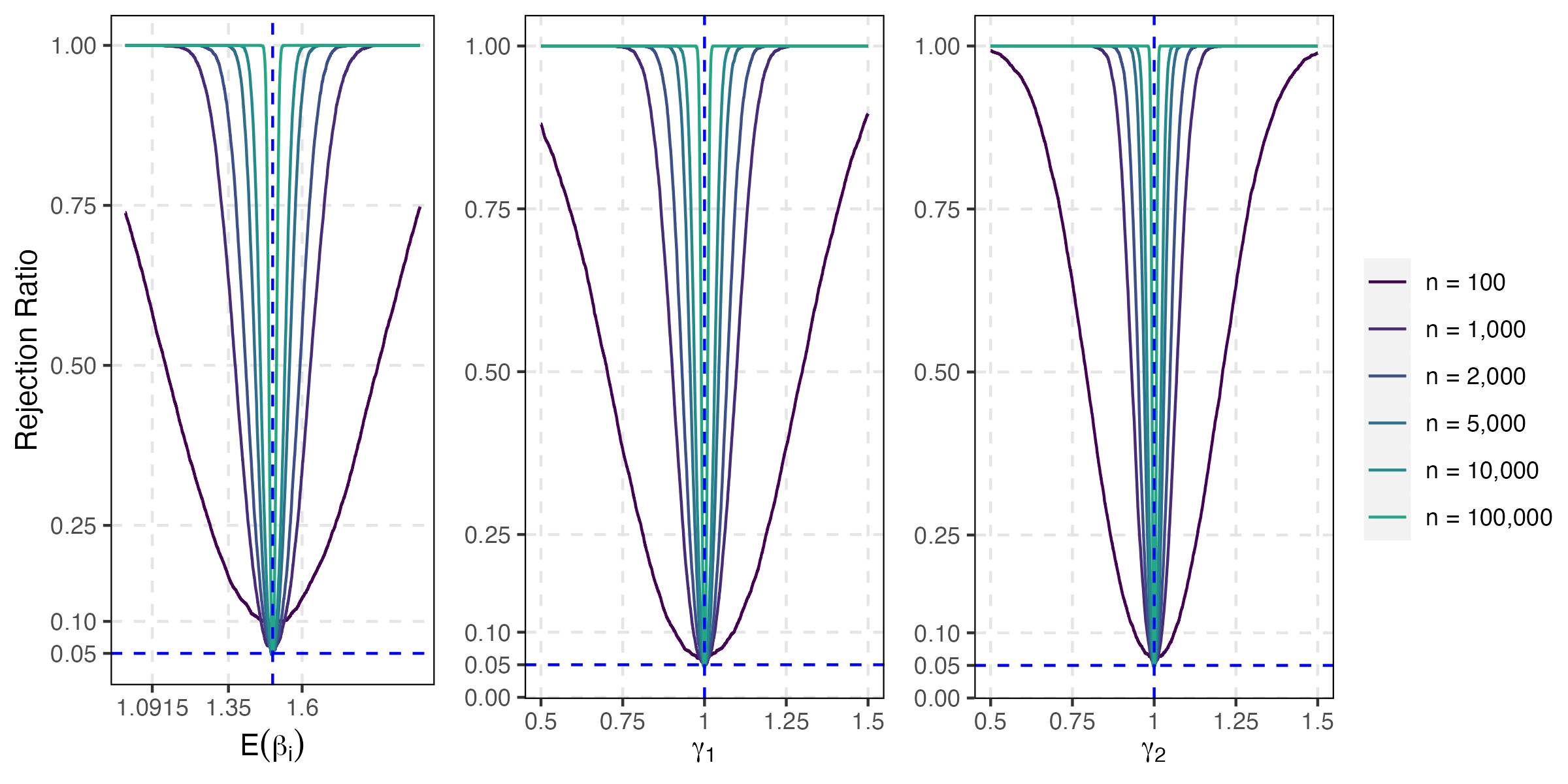
(a) Baseline

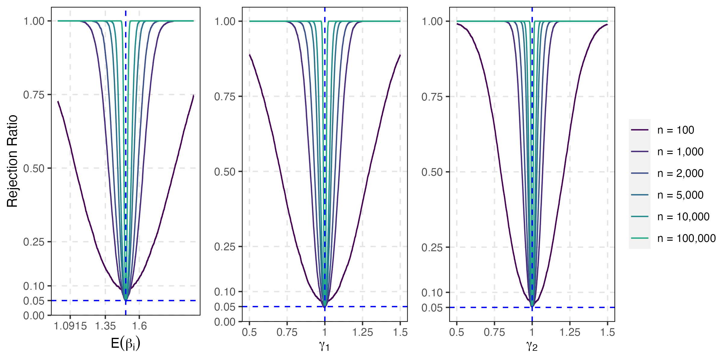
(b) Categorical $x$

(c) Categorical $u$

Notes: The data generating process is (5.1) with high variance parametrization that is described in (5.2). “Baseline”, “Categorical $x$” and “Categorical $u$” refer to DGP 1 to 3 as in Section 5.1. Generically, power is calculated by $R^{-1}\sum_{r=1}^{R}\mathbf{1}\left[\left|\hat{\theta}^{(r)}-\theta_{\delta}\right|/\hat{\sigma}_{\hat{\theta}}^{(r)}>\mathrm{cv}_{0.05}\right]$, for $\theta_{\delta}$ in a symmetric neighborhood of the true parameter $\theta_{0}$, the estimate $\hat{\theta}^{(r)}$, the estimated standard error of $\hat{\theta}^{(r)}$, $\hat{\sigma}_{\hat{\theta}}^{(r)}$, and the critical value $\mathrm{cv}_{0.05}=\Phi^{-1}\left(0.975\right)$ across $R=5,000$ replications, where $\Phi\left(\cdot\right)$ is the cumulative distribution function of standard normal distribution.

Figure 2: Empirical power functions for the least square estimator $\hat{\mathbf{\phi}}$ with the low variance parametrization ($\mathrm{var}\left(\beta_{i}\right)=0.15$)

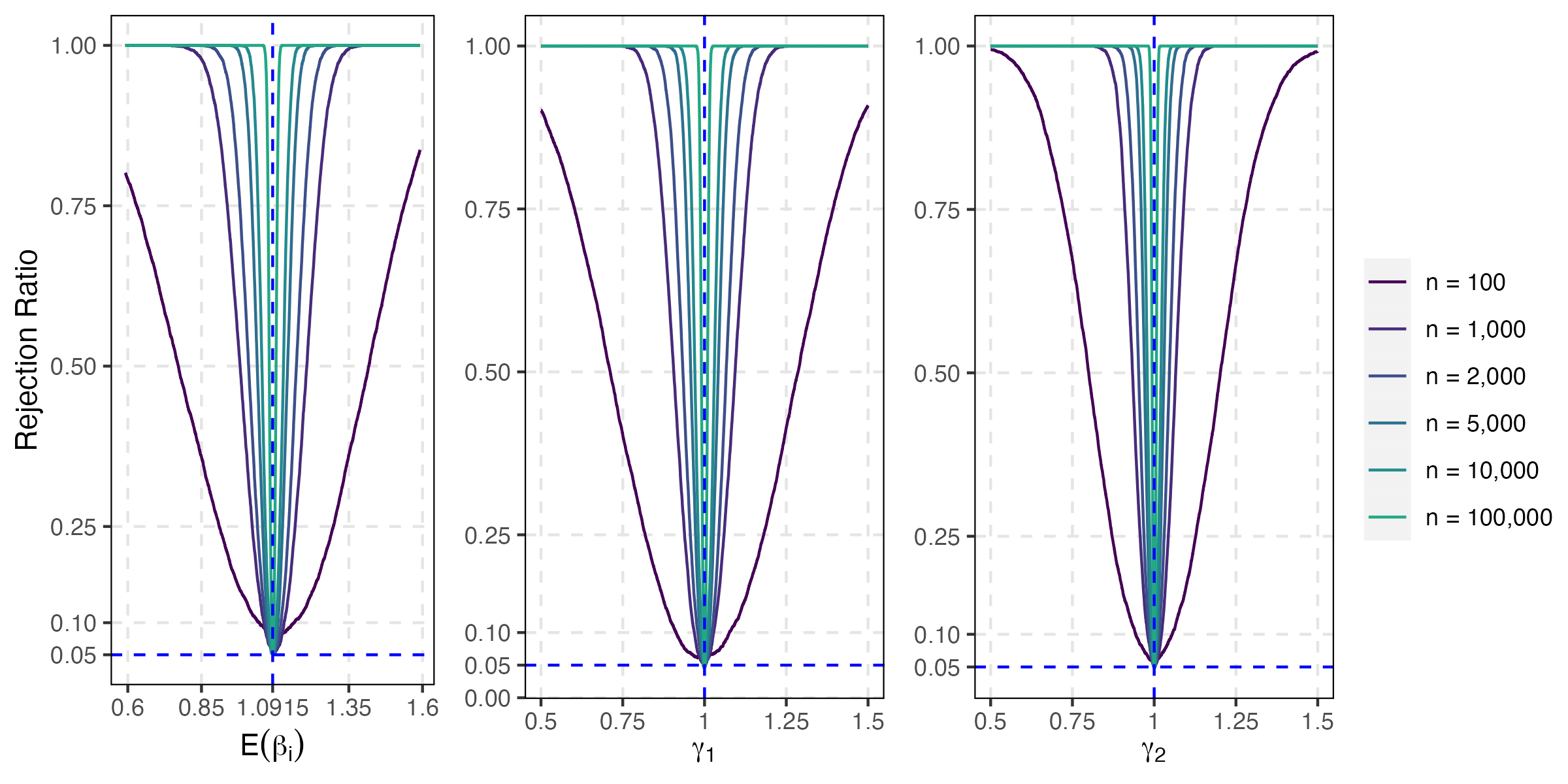
(a) Baseline

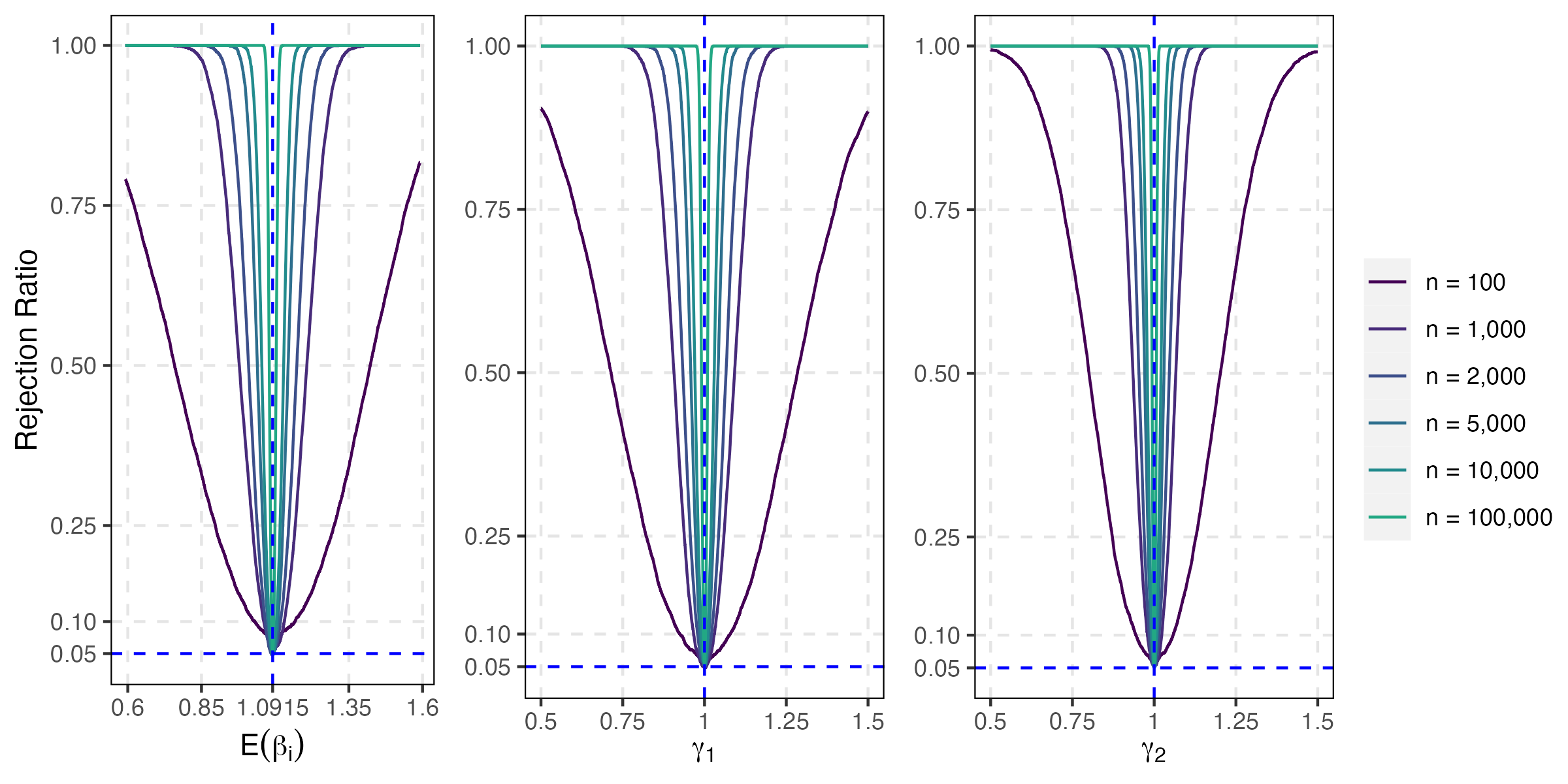
(b) Categorical $x$

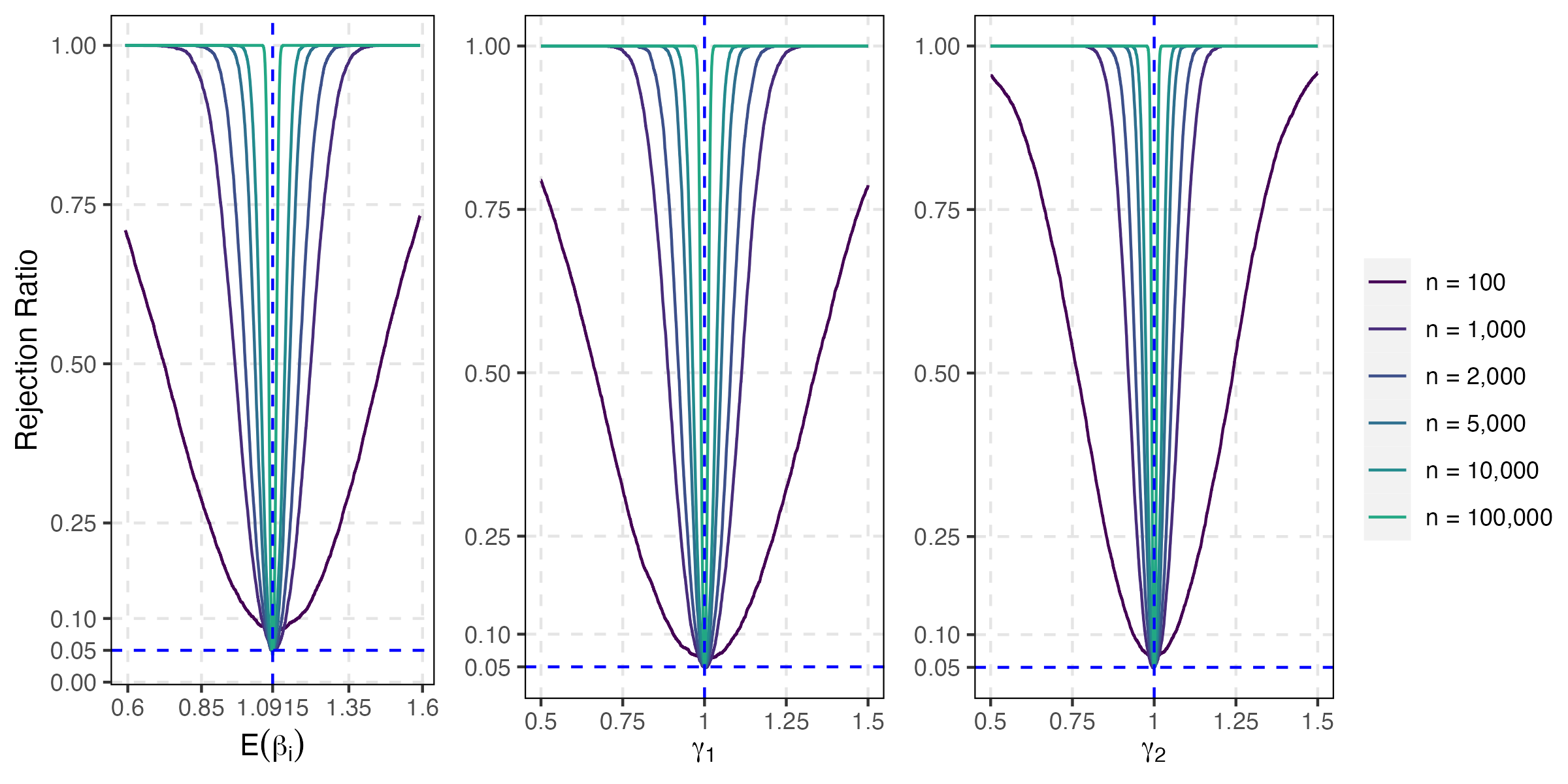
(c) Categorical $u$

Notes: The data generating process is (5.1) with low variance parametrization that is described in (5.2). “Baseline”, “Categorical $x$” and “Categorical $u$” refer to DGP 1 to 3 as in Section 5.1. Generically, power is calculated by $R^{-1}\sum_{r=1}^{R}\mathbf{1}\left[\left|\hat{\theta}^{(r)}-\theta_{\delta}\right|/\hat{\sigma}_{\hat{\theta}}^{(r)}>\mathrm{cv}_{0.05}\right]$, for $\theta_{\delta}$ in a symmetric neighborhood of the true parameter $\theta_{0}$, the estimate $\hat{\theta}^{(r)}$, the estimated standard error of $\hat{\theta}^{(r)}$, $\hat{\sigma}_{\hat{\theta}}^{(r)}$, and the critical value $\mathrm{cv}_{0.05}=\Phi^{-1}\left(0.975\right)$ across $R=5,000$ replications, where $\Phi\left(\cdot\right)$ is the cumulative distribution function of standard normal distribution.

Table 3: Bias, RMSE and size of the GMM estimator for distributional parameters of $\beta$

DGP		Baseline			Categorical $x$			Categorical $u$
Sample size $n$		Bias	RMSE	Size	Bias	RMSE	Size	Bias	RMSE	Size
high variance: $\mathrm{var}\left(\beta_{i}\right)=0.25$
$\pi=0.5$	100	0.0457	0.2291	0.1737	0.0363	0.2410	0.2130	0.0235	0.2361	0.2231
	1,000	0.0018	0.1019	0.1308	0.0033	0.1178	0.1437	-0.0270	0.1741	0.2033
	2,000	0.0017	0.0688	0.1084	0.0015	0.0826	0.1199	-0.0174	0.1273	0.1545
	5,000	-0.0003	0.0416	0.0936	-0.0015	0.0495	0.0908	-0.0089	0.0810	0.1048
	10,000	0.0002	0.0301	0.0774	-0.0006	0.0351	0.0780	-0.0052	0.0582	0.0864
	100,000	-0.0001	0.0096	0.0550	0.0002	0.0114	0.0576	-0.0009	0.0194	0.0582
$\beta_{L}=1$	100	0.1415	0.4749	0.2472	0.1099	0.5110	0.2138	0.1151	0.5961	0.1820
	1,000	0.0207	0.1242	0.1501	0.0200	0.1454	0.1433	-0.0256	0.2373	0.1225
	2,000	0.0129	0.0819	0.1344	0.0116	0.1007	0.1355	-0.0094	0.1486	0.1094
	5,000	0.0048	0.0512	0.1052	0.0027	0.0607	0.1000	-0.0053	0.0897	0.0850
	10,000	0.0031	0.0365	0.0854	0.0021	0.0428	0.0900	-0.0020	0.0633	0.0714
	100,000	0.0002	0.0112	0.0534	0.0007	0.0135	0.0584	-0.0002	0.0207	0.0574
$\beta_{H}=2$	100	-0.0996	0.5609	0.2014	-0.0873	0.6154	0.1963	-0.1071	0.6996	0.1866
	1,000	-0.0193	0.1407	0.1864	-0.0128	0.1581	0.1661	-0.0319	0.2400	0.2093
	2,000	-0.0099	0.0893	0.1486	-0.0099	0.1094	0.1467	-0.0239	0.1663	0.1673
	5,000	-0.0053	0.0519	0.1092	-0.0072	0.0622	0.1082	-0.0127	0.1019	0.1156
	10,000	-0.0020	0.0362	0.0878	-0.0033	0.0430	0.0880	-0.0080	0.0718	0.0986
	100,000	-0.0005	0.0114	0.0530	-0.0003	0.0134	0.0548	-0.0017	0.0236	0.0646
low variance: $\mathrm{var}\left(\beta_{i}\right)=0.15$
$\pi=0.3$	100	0.2175	0.3084	0.2183	0.2227	0.3187	0.2464	0.2294	0.3157	0.2500
	1,000	0.0170	0.1536	0.1873	0.0307	0.1837	0.2063	0.0511	0.2295	0.2493
	2,000	0.0014	0.1010	0.1426	0.0105	0.1290	0.1601	0.0181	0.1815	0.2102
	5,000	-0.0002	0.0590	0.1084	0.0010	0.0737	0.1158	0.0085	0.1232	0.1468
	10,000	-0.0001	0.0415	0.0894	0.0005	0.0515	0.0928	0.0067	0.0906	0.1046
	100,000	-0.0001	0.0129	0.0594	0.0003	0.0158	0.0536	0.0108	0.0349	0.0776
$\beta_{L}=0.5$	100	0.3365	0.5905	0.2426	0.3153	0.6042	0.2432	0.3384	0.6746	0.2005
	1,000	0.0352	0.2334	0.1560	0.0290	0.2813	0.1544	0.0131	0.4141	0.1233
	2,000	0.0175	0.1414	0.1310	0.0131	0.1835	0.1382	-0.0157	0.2988	0.1037
	5,000	0.0085	0.0830	0.1082	0.0041	0.1052	0.1118	-0.0057	0.1798	0.0928
	10,000	0.0055	0.0577	0.0966	0.0031	0.0730	0.0934	0.0019	0.1231	0.0760
	100,000	0.0005	0.0180	0.0596	0.0011	0.0222	0.0582	0.0130	0.0443	0.0962
$\beta_{H}=1.345$	100	0.0023	0.4727	0.1377	0.0238	0.5290	0.1453	0.0185	0.6500	0.1461
	1,000	-0.0081	0.1265	0.1737	0.0042	0.1621	0.1655	0.0120	0.2353	0.1738
	2,000	-0.0092	0.0828	0.1428	-0.0026	0.1045	0.1475	0.0029	0.1607	0.1710
	5,000	-0.0048	0.0489	0.1028	-0.0041	0.0586	0.1034	0.0006	0.0970	0.1172
	10,000	-0.0025	0.0340	0.0808	-0.0024	0.0412	0.0942	0.0019	0.0706	0.0958
	100,000	-0.0004	0.0105	0.0486	-0.0002	0.0125	0.0548	0.0073	0.0262	0.0696

Notes: The data generating process is (5.1). high variance and low variance parametrization are described in (5.2). “Baseline”, “Categorical $x$” and “Categorical $u$” refer to DGP 1 to 3 as in Section 5.1. Generically, bias, RMSE and size are calculated by $R^{-1}\sum_{r=1}^{R}\left(\hat{\theta}^{(r)}-\theta_{0}\right)$, $\sqrt{R^{-1}\sum_{r=1}^{R}\left(\hat{\theta}^{(r)}-\theta_{0}\right)^{2}}$, and $R^{-1}\sum_{r=1}^{R}\mathbf{1}\left[\left|\hat{\theta}^{(r)}-\theta_{0}\right|/\hat{\sigma}_{\hat{\theta}}^{(r)}>\mathrm{cv}_{0.05}\right]$, respectively, for true parameter $\theta_{0}$, its estimate $\hat{\theta}^{(r)}$, the estimated standard error of $\hat{\theta}^{(r)}$, $\hat{\sigma}_{\hat{\theta}}^{(r)}$, and the critical value $\mathrm{cv}_{0.05}=\Phi^{-1}\left(0.975\right)$ across $R=5,000$ replications, where $\Phi\left(\cdot\right)$ is the cumulative distribution function of standard normal distribution.

Figure 3: Empirical power functions for the GMM estimator of distributional parameters of $\beta$ with the high variance parametrization($\mathrm{var}\left(\beta_{i}\right)=0.25$)

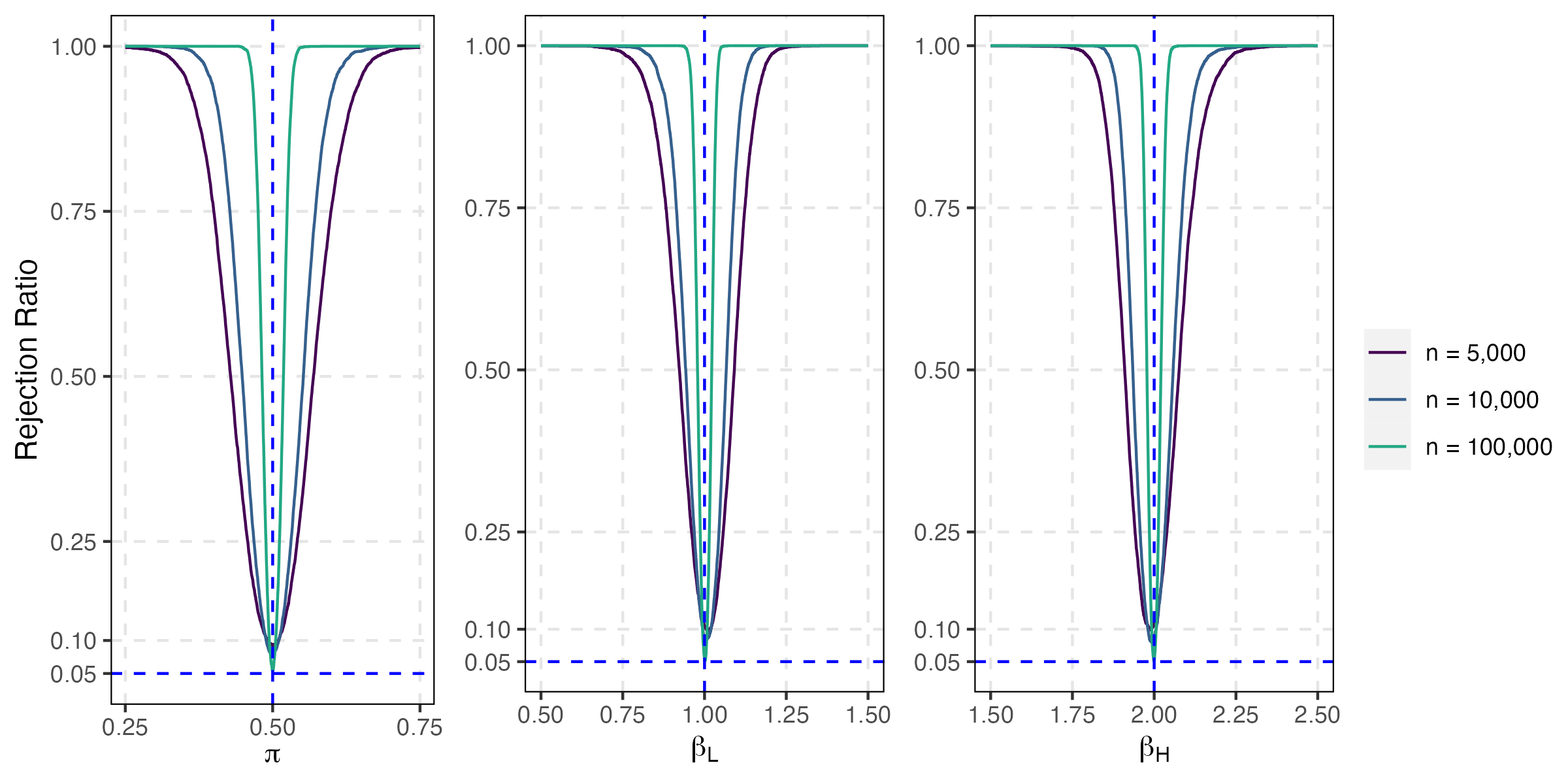
(a) Baseline

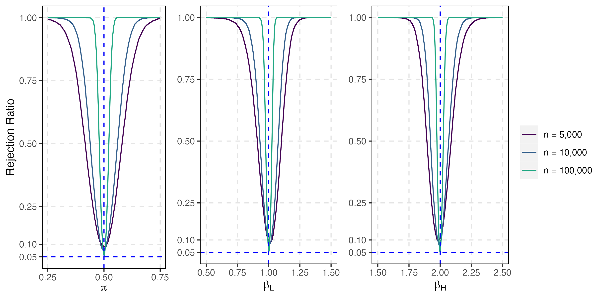
(b) Categorical $x$

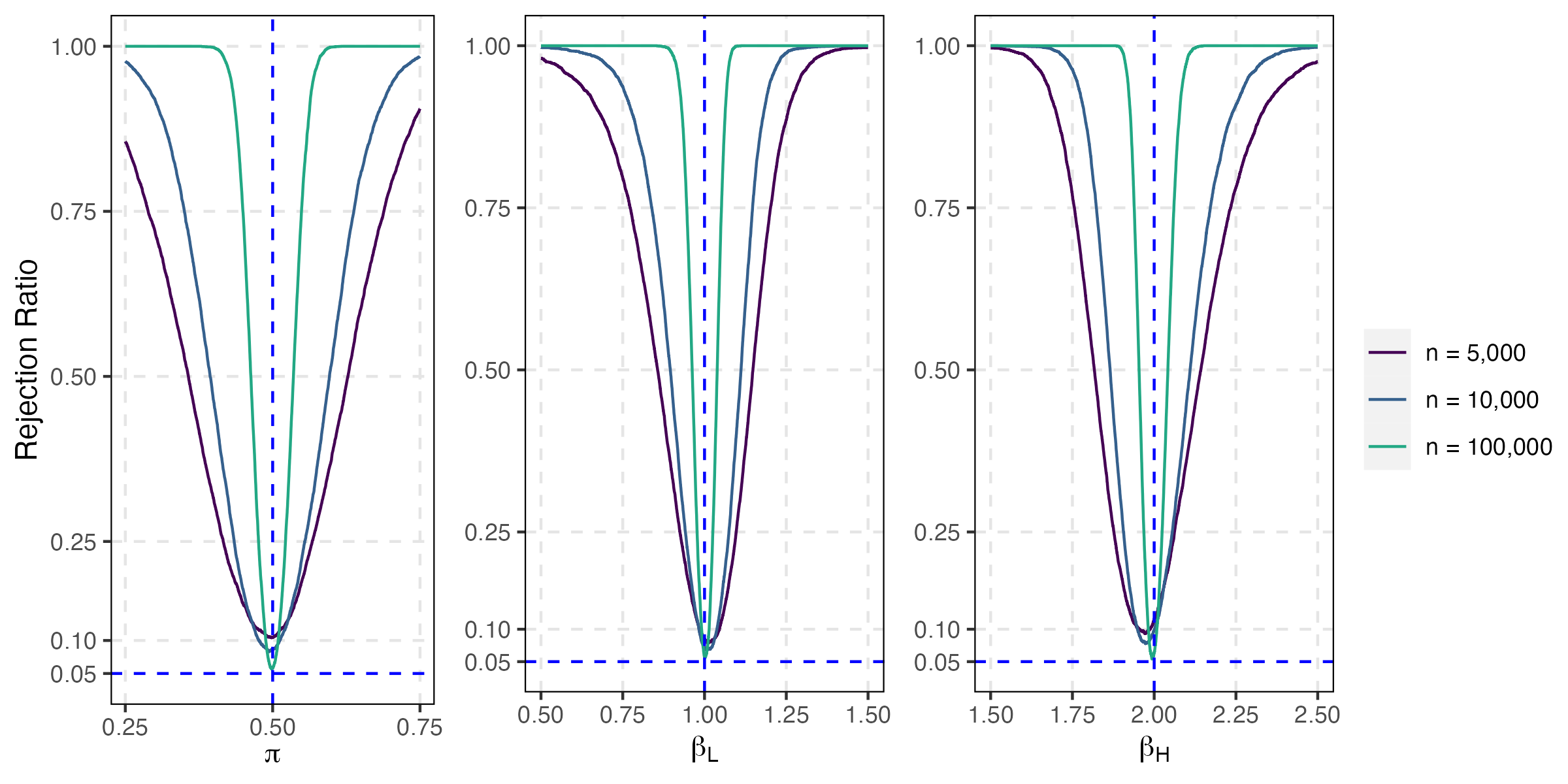
(c) Categorical $u$

Notes: The data generating process is (5.1) with high variance parametrization that is described in (5.2). “Baseline”, “Categorical $x$” and “Categorical $u$” refer to DGP 1 to 3 as in Section 5.1. The model is estimated with $S=4$, the highest order of moments of $x_{i}$ used in estimation. Generically, power is calculated by $R^{-1}\sum_{r=1}^{R}\mathbf{1}\left[\left|\hat{\theta}^{(r)}-\theta_{\delta}\right|/\hat{\sigma}_{\hat{\theta}}^{(r)}>\mathrm{cv}_{0.05}\right]$, for $\theta_{\delta}$ in a symmetric neighborhood of the true parameter $\theta_{0}$, the estimate $\hat{\theta}^{(r)}$, the estimated standard error of $\hat{\theta}^{(r)}$, $\hat{\sigma}_{\hat{\theta}}^{(r)}$, and the critical value $\mathrm{cv}_{0.05}=\Phi^{-1}\left(0.975\right)$ across $R=5,000$ replications, where $\Phi\left(\cdot\right)$ is the cumulative distribution function of standard normal distribution.

Figure 4: Empirical power functions for the GMM estimator of distributional parameters of $\beta$ with the low variance parametrization ($\mathrm{var}\left(\beta_{i}\right)=0.15$)

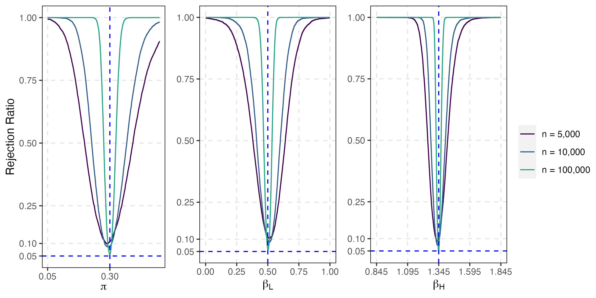
(a) Baseline

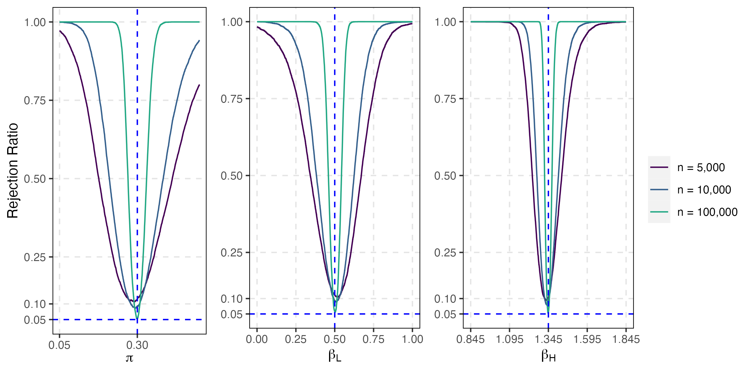
(b) Categorical $x$

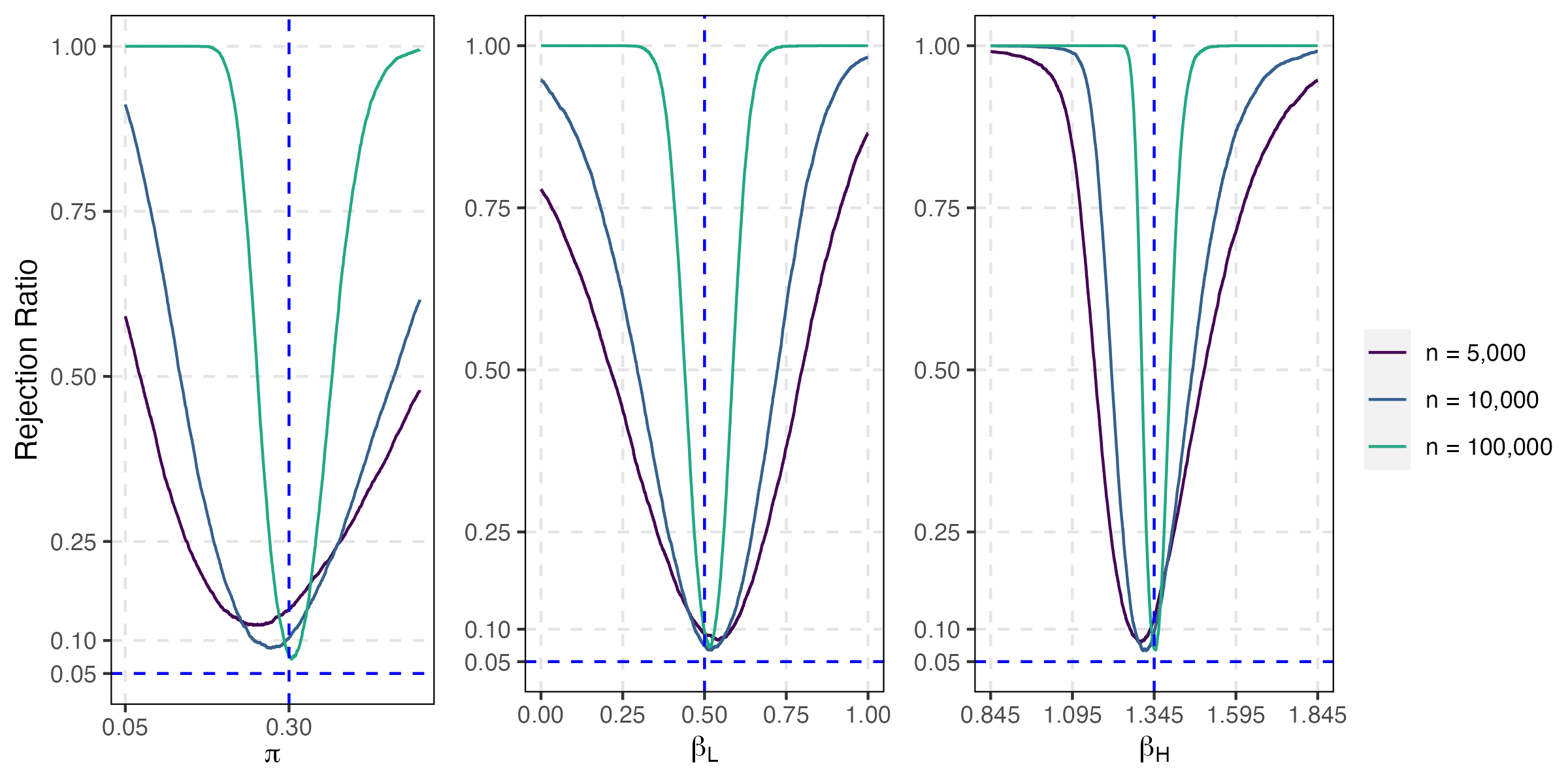
(c) Categorical $u$

Notes: The data generating process is (5.1) with low variance parametrization that is described in (5.2). “Baseline”, “Categorical $x$” and “Categorical $u$” refer to DGP 1 to 3 as in Section 5.1. The model is estimated with $S=4$, the highest order of moments of $x_{i}$ used in estimation. Generically, power is calculated by $R^{-1}\sum_{r=1}^{R}\mathbf{1}\left[\left|\hat{\theta}^{(r)}-\theta_{\delta}\right|/\hat{\sigma}_{\hat{\theta}}^{(r)}>\mathrm{cv}_{0.05}\right]$, for $\theta_{\delta}$ in a symmetric neighborhood of the true parameter $\theta_{0}$, the estimate $\hat{\theta}^{(r)}$, the estimated standard error of $\hat{\theta}^{(r)}$, $\hat{\sigma}_{\hat{\theta}}^{(r)}$, and the critical value $\mathrm{cv}_{0.05}=\Phi^{-1}\left(0.975\right)$ across $R=5,000$ replications, where $\Phi\left(\cdot\right)$ is the cumulative distribution function of standard normal distribution.

For each sample size $n=100$, $1,000$, $2,000$, $5,000$, $10,000$ and $100,000$ we run $5,000$ replications of experiments for DGP 1 (baseline), DGP 2 (categorical $x$) and DGP 3 (categorical $u$) with high variance and low variance parametrization, as set out in (5.2).

We first investigate the finite sample performance of $\hat{\mathbf{\phi}}$, as an estimator of $\mathbf{\phi}=\left(\mathrm{E}\left(\beta_{i}\right),\mathbf{\gamma}^{\prime}\right)^{\prime}$. Bias, root mean squared errors (RMSE) for estimation of $\mathrm{E}\left(\beta_{i}\right)$, $\gamma_{1}$ and $\gamma_{2}$, as well as size of testing of the null values at the 5 per cent nominal value are reported in Table 2. In addition, we plot the associated empirical power functions in Figure 1 and 2, for cases of high and low $var(\beta_{i})$. The results show that $\hat{\mathbf{\phi}}$ has very good small sample properties with small bias and RMSEs, with size very close to the nominal value of 5 per cent across all DGPs and parametrization, even when sample size is relatively small. The power of the test increases steadily as the sample size increases.

Then, we turn to the GMM estimator for the distributional parameters of $\beta_{i}$ proposed in Section 3.2. The bias, RMSE, and the test size based on the asymptotic distribution given in Theorem 5, for $\pi$, $\beta_{L}$ and $\beta_{H}$, are reported in Table 3. The empirical power functions are reported in Figure 3 and 4. The reported results are based on $S=4$, where $S$ $(>2K-1=3)$ denotes the highest order of moments of $x_{i}$ included in estimation.

The upper panel of this table reports the results of the high variance and the lower panel for the low variance parametrization, as set out in (5.2). For all parameters and under all DGPs, the bias and RMSE decline steadily with the sample size as predicted by Theorem 4, and confirm the robustness of the GMM estimates to the heterogeneity in the regressor and the error processes. But for a given sample size, the relative precision of the estimates depends on the variability of $\beta_{i}$, as characterized by the true value of $\mathrm{var}(\beta_{i})$. The precision of the estimates with high variance parametrization is relatively higher than that with low variance parametrization. This is to be expected since, unlike $\mathrm{E}(\beta_{i}),$ the distributional parameters are only identified if $\mathrm{var}(\beta_{i})>0$. As shown in (2.18) and (2.19) for the current case of $K=2$, $\mathrm{var}(\beta_{i})$ is in the denominator when we recover the distributional parameters from the moments of $\beta_{i}$. When $\mathrm{var}(\beta_{i})$ is small, estimation errors in the moments of $\beta_{i}$ can be amplified in the estimation of $\pi$, $\beta_{L}$ and $\beta_{H}$. On the other hand, the larger the variance the more precisely $\pi$, $\beta_{H}$ and $\beta_{L}$ can be estimated for a given $n$. The size and power also depends on the parametrization. With both high variance and low variance parametrization, we can achieve correct size and reasonable power when $n$ is quite large ($n=100,000$). We plot the empirical power functions for $n\geq 5,000$ for $\pi$, $\beta_{H}$ and $\beta_{L}$ since the size is far above 5 per cent for smaller values of $n$, and power comparisons are not meaningful in such cases.

Remark 15

Note that GMM estimators of moments of $\beta_{i}$, namely $\mathbf{m}_{\mathbf{\beta}}$, can be obtained using the moment conditions in (3.7),and the transformations $\mathbf{m}_{\mathbf{\beta}}=h\left(\mathbf{\theta}\right)$ in (3.4) are required only to derive the estimators of $\mathbf{\theta}$, the parameters of the underlying categorical distribution. The Monte Carlo results in Section S.3.2 in the online supplement show that $\mathbf{m}_{\mathbf{\beta}}$ can be accurately estimated with relatively small sample sizes. In the estimation of both $\mathbf{m}_{\mathbf{\beta}}$ and $\mathbf{\theta}$, the same set of moment conditions are included, so the estimation of distributional parameters $\mathbf{\theta}$ essentially relies on the relation $\mathbf{\theta}=h^{-1}\left(\mathbf{m}_{\mathbf{\beta}}\right)$. Sampling uncertainties in the estimation of $\mathbf{m}_{\mathbf{\beta}}$, particularly in higher order moments, are potentially amplified through the inverse transformation $h^{-1}$ that involves matrix inversion, which causes the difficulties in estimation and inference of $\mathbf{\theta}$ when sample sizes are small. This is analogous to the problem of precision matrix estimation from an estimated covariance matrix. In practice, estimation of the categorical parameters is recommended for applications where the sample size is relatively large, otherwise it is advisable to focus on estimates of the lower order moments of $\beta_{i}$.

6 Heterogeneous return to education: An empirical application

Since the pioneering work by Becker (1962, 1964) on the effects of investments in human capital, estimating returns to education has been one of the focal points of labor economics research. In his pioneering contribution Mincer (1974) models the logarithm of earnings as a function of years of education and years of potential labor market experience (age minus years of education minus six), which can be written in a generic form:

$$\log\text{wage}_{i}=\alpha_{i}+\beta_{i}\text{edu}_{i}+\phi\left(\mathbf{z}_{i}\right)+\varepsilon_{i},$$ (6.1)

as in Heckman, Humphries, and Veramendi (2018, Equation (1)), where $\mathbf{z}_{i}$ includes the labor market experience and other relevant control variables. The above wage equation, also known as the “Mincer equation”, has become of the workhorse of the empirical works on estimating the return to education. In the most widely used specification of the Mincer equation (6.1),

$$\phi\left(\mathbf{z}_{i}\right)=\rho_{1}\text{exper}_{i}+\rho_{2}\text{exper}_{i}^{2}+\tilde{\mathbf{z}}_{i}^{\prime}\tilde{\mathbf{\gamma}},$$

where $\tilde{\mathbf{z}}_{i}$ is the vector of control variables other than potential labor market experience.

Along with the advancement of empirical research on this topic, there has been a growing awareness of the importance of heterogeneity in individual cognitive and non-cognitive abilities (Heckman, 2001) and their significance for explaining the observed heterogeneity in return to education. Accordingly, it is important to allow the parameters of the wage equation to differ across individuals. In equation (6.1) we allow $\alpha_{i}$ and $\beta_{i}$ to differ across individuals, but assume that $\phi\left(\mathbf{z}_{i}\right)$ can be approximated as non-linear functions of experience and other control variables with homogeneous coefficients.

Specifically, following Lemieux (2006b, c) we also allow for time variations in the parameters of the wage equation and consider the following categorical coefficient model over a given cross-section sample indexed by $t$:

$$\log\text{wage}_{it}=\alpha_{it}+\beta_{it}\text{edu}_{it}+\rho_{1t}\text{exper}_{it}+\rho_{2t}\text{exper}_{it}^{2}+\tilde{\mathbf{z}}_{it}^{\prime}\tilde{\mathbf{\gamma}}_{t}+\varepsilon_{it},$$ (6.2)

where the return to education follows the categorical distribution,

$$\beta_{it}=\begin{cases}b_{tL}&\text{w.p. }\pi_{t},\\ b_{tH}&\text{w.p. }1-\pi_{t},\end{cases}$$

and $\tilde{\mathbf{z}}_{it}$ includes gender, martial status and race. $\alpha_{it}=\alpha_{t}+\delta_{it}$ where $\delta_{it}$ is mean $0$ random variable assumed to be distributed independently of $\text{edu}_{it}$ and $\mathbf{z}_{it}=\left(\text{exper}_{it},\text{exper}_{it}^{2}\text{, }\tilde{\mathbf{z}}_{t}^{\prime}\right)^{\prime}$. Let $u_{it}=\varepsilon_{it}+\delta_{it}$, and write (6.2) as

$$\log\text{wage}_{it}=\alpha_{t}+\beta_{it}\text{edu}_{it}+\rho_{1t}\text{exper}_{it}+\rho_{2t}\text{exper}_{it}^{2}+\tilde{\mathbf{z}}_{it}^{\prime}\tilde{\mathbf{\gamma}}_{t}+u_{it}.$$ (6.3)

The correlation between $\alpha_{it}$ and $\text{edu}_{it}$ in (6.1) is the source of “ability bias” (Griliches, 1977). Given the pure cross-sectional nature of our analysis, we do not allow for the endogeneity from “ability bias” or dynamics. To allow for non-zero correlations between $\alpha_{it}$, edu_it and $\mathbf{z}_{it}$, a panel data approach is required, which has its own challenges, as education and experience variables tend to very slow moving (if at all) for many individuals in the panel. Time delays between changes in education and experience, and the wage outcomes also further complicate the interpretation of the mean estimates of $\beta_{it}$ which we shall be reporting. To partially address the possible dynamic spillover effects, we provide estimates of the distribution of $\beta_{it}$ using cross-sectional data from two different sample periods, and investigate the extent to which the distribution of return to education has changed over time, by gender and the level of educational achievements.

We estimate the categorical distribution of the return to education in (6.3) using the May and Outgoing Rotation Group (ORG) supplements of the Current Population Survey (CPS) data, as in Lemieux (2006b, c). We pool observations from 1973 to 1975 for the first sample period, $t=\left\{1973-1975\right\}$ and observations from 2001 to 2003 for the second sample period, $t=\left\{2001-2003\right\}$. Following Lemieux (2006b), we consider sub-samples of those with less than 12 years of education, “high school or less”, and those with more than 12 years of education, “postsecondary education”, as well as the combined sample. We also present results by gender. The summary statistics are reported in Table 4. As to be expected, the mean log wages are higher for those with postsecondary education (for male and female), with the number of years of schooling and experience rising by about one year across the two sub-period samples. There are also important differences across male and female, and the two educational groupings, which we hope to capture in our estimation.

Table 4: Summary Statistics of the May and Outgoing Rotation Group (ORG) supplements of the Current Population Survey (CPS) data across two periods, 1973 - 75 and 2001 - 03, by years of education and gender

	1973 - 75				2001 - 03
	High School	Postsecondary	All		High School	Postsecondary	All
	or Less	Education			or Less	Education
	Both male and female
log wage	1.59	1.94	1.69		1.47	1.88	1.71
	(0.50)	(0.53)	(0.53)		(0.47)	(0.57)	(0.57)
edu.	10.64	15.21	12.02		11.29	14.96	13.41
	(2.11)	(1.65)	(2.89)		(1.68)	(1.82)	(2.53)
age	36.74	34.90	36.18		37.96	39.87	39.06
	(13.85)	(11.58)	(13.23)		(12.93)	(11.33)	(12.07)
expr.	20.10	13.69	18.17		20.67	18.91	19.65
	(14.44)	(11.41)	(13.91)		(12.95)	(11.17)	(11.98)
marriage	0.67	0.70	0.68		0.52	0.60	0.57
	(0.47)	(0.46)	(0.47)		(0.50)	(0.49)	(0.50)
nonwhite	0.11	0.08	0.10		0.15	0.14	0.15
	(0.32)	(0.27)	(0.30)		(0.36)	(0.35)	(0.35)
$n$	77,899	33,733	111,632		216,136	295,683	511,819
	Male
log wage	1.76	2.07	1.86		1.57	2.00	1.81
	(0.48)	(0.53)	(0.52)		(0.48)	(0.58)	(0.58)
edu.	10.44	15.29	12.00		11.19	15.02	13.31
	(2.26)	(1.69)	(3.08)		(1.82)	(1.84)	(2.64)
age	36.79	35.29	36.31		37.21	40.24	38.89
	(13.82)	(11.24)	(13.07)		(12.70)	(11.30)	(12.04)
expr.	20.35	14.00	18.32		20.02	19.22	19.58
	(14.49)	(11.06)	(13.81)		(12.75)	(11.08)	(11.86)
marriage	0.73	0.76	0.74		0.53	0.64	0.59
	(0.44)	(0.43)	(0.44)		(0.50)	(0.48)	(0.49)
nonwhite	0.10	0.06	0.09		0.14	0.13	0.13
	(0.30)	(0.24)	(0.29)		(0.34)	(0.33)	(0.34)
$n$	44,299	20,851	65,150		116,129	144,138	260,267
	Female
log wage	1.35	1.71	1.45		1.77	1.36	1.61
	(0.41)	(0.47)	(0.46)		(0.54)	(0.43)	(0.54)
edu.	10.89	15.08	12.05		14.90	11.42	13.52
	(1.87)	(1.59)	(2.60)		(1.79)	(1.49)	(2.40)
age	36.67	34.27	36.01		38.83	39.52	39.24
	(13.88)	(12.09)	(13.45)		(13.14)	(11.35)	(12.10)
expr.	19.78	13.19	17.96		18.61	21.41	19.73
	(14.36)	(11.94)	(14.04)		(11.24)	(13.13)	(12.11)
marriage	0.60	0.60	0.60		0.56	0.51	0.54
	(0.49)	(0.49)	(0.49)		(0.50)	(0.50)	(0.50)
nonwhite	0.13	0.10	0.12		0.15	0.17	0.16
	(0.33)	(0.30)	(0.33)		(0.36)	(0.38)	(0.37)
$n$	33,600	12,882	46,482		151,545	100,007	251,552

Notes: “Postsecondary Education” stands for the sub-sample with years of education higher than 12 and “High School or Less” stands for sub-sample with years of education less than or equal to 12). edu. and exper. are in years. marriage and nonwhite are dummy variables. $n$ is the sample size. We report mean and standard deviation (in parentheses) of each variable. The data is from the May and Outgoing Rotation Group (ORG) supplements of the Current Population Survey (CPS) data retrived from https://www.openicpsr.org/openicpsr/project/116216/version/V1/view.

Table 5: Estimates of the distribution of the return to education across two periods, 1973 - 75 and 2001 - 03, by years of education and gender

	High School or Less			Postsecondary Edu.			All
	1973 - 75	2001 - 03		1973 - 75	2001 - 03		1973 - 75	2001 - 03
	Both Male and Female
$\pi$	0.4843	0.5069		0.4398	0.3537		0.4719	0.3463
	(4188.8)	(0.0269)		(0.0502)	(0.0091)		(0.0485)	(0.0047)
$\beta_{L}$	0.0608	0.0382		0.0624	0.0866		0.0558	0.0645
	(5.0939)	(0.0014)		(0.0035)	(0.0009)		(0.0020)	(0.0004)
$\beta_{H}$	0.0619	0.0920		0.1103	0.1401		0.0941	0.1263
	(4.8132)	(0.0019)		(0.0032)	(0.0007)		(0.0022)	(0.0004)
$\beta_{H}/\beta_{L}$	1.0194	2.4102		1.7680	1.6178		1.6879	1.9567
	(6.2938)	(0.0428)		(0.0618)	(0.0111)		(0.0295)	(0.0080)
$\mathrm{E}\left(\beta_{i}\right)$	0.0614	0.0647		0.0893	0.1212		0.0760	0.1049
$\mathrm{s.d.}\left(\beta_{i}\right)$	0.0006	0.0269		0.0238	0.0256		0.0191	0.0294
$n$	77,899	216,136		33,733	295,683		111,632	511,819
	Male
$\pi$	n/a	0.4939		0.4706	0.3201		0.4802	0.3290
	n/a	(0.0399)		(0.0707)	(0.0104)		(0.0815)	(0.0053)
$\beta_{L}$	0.0637	0.0404		0.0534	0.0743		0.0536	0.0548
	n/a	(0.0019)		(0.0046)	(0.0012)		(0.0030)	(0.0005)
$\beta_{H}$	0.0637	0.0911		0.0995	0.1308		0.0875	0.1192
	n/a	(0.0026)		(0.0042)	(0.0009)		(0.0031)	(0.0005)
$\beta_{H}/\beta_{L}$	1.0000	2.2526		1.8641	1.7603		1.6312	2.1772
	n/a	(0.0534)		(0.1038)	(0.0209)		(0.0459)	(0.0144)
$\mathrm{E}\left(\beta_{i}\right)$	0.0637	0.0661		0.0778	0.1128		0.0712	0.0980
$\mathrm{s.d.}\left(\beta_{i}\right)$	0.0000	0.0253		0.0230	0.0264		0.0169	0.0303
$n$	44,299	116,129		20,851	144,138		65,150	260,267
	Female
$\pi$	0.4999	0.5166		0.4526	0.3906		0.4566	0.3608
	(0.5047)	(0.0283)		(0.0829)	(0.0167)		(0.0810)	(0.0086)
$\beta_{L}$	0.0441	0.0348		0.0823	0.0979		0.0628	0.0751
	(0.0133)	(0.0016)		(0.0053)	(0.0013)		(0.0033)	(0.0007)
$\beta_{H}$	0.0723	0.0972		0.1310	0.1473		0.1028	0.1333
	(0.0159)	(0.0025)		(0.0055)	(0.0011)		(0.0038)	(0.0007)
$\beta_{H}/\beta_{L}$	1.6392	2.7934		1.5913	1.5048		1.6357	1.7756
	(0.1565)	(0.0700)		(0.0539)	(0.0121)		(0.0353)	(0.0090)
$\mathrm{E}\left(\beta_{i}\right)$	0.0582	0.0650		0.1090	0.1280		0.0845	0.1123
$\mathrm{s.d.}\left(\beta_{i}\right)$	0.0141	0.0312		0.0242	0.0241		0.0199	0.0280
$n$	33,600	100,007		12,882	151,545		46,482	251,552

Notes: This table reports the estimates of the distribution of $\beta_{i}$ with the quadratic in experience specification (6.2), using $S=4$ order moments of $\text{edu}_{i}$. “Postsecondary Edu.” stands for the sub-sample with years of education higher than 12 and “High School or Less” stands for those with years of education less than or equal to 12. $\mathrm{s.d.}\left(\beta_{i}\right)$ corresponds to the square root of estimated $\mathrm{var}\left(\beta_{i}\right)$. $n$ is the sample size. “n/a” is inserted when the estimates show homogeneity of $\beta_{i}$ and $\pi$ is not identified and cannot be estimated.

Table 6: Estimates of $\mathbf{\gamma}$ associated with control variables $\mathbf{z}_{i}$ with specification (6.2) across two periods, 1973 - 75 and 2001 - 03, by years of education and gender, which complements Table 5

	High School or Less			Postsecondary Edu.			All
	1973 - 75	2001 - 03		1973 - 75	2001 - 03		1973 - 75	2001 - 03
	Both male and female
exper.	0.0305	0.0319		0.0415	0.0354		0.0310	0.0321
	(0.0004)	(0.0002)		(0.0008)	(0.0003)		(0.0003)	(0.0002)
$\mathtt{exper.}^{2}$ ($\times 10^{2}$)	-0.0490	-0.0505		-0.0826	-0.0652		-0.0499	-0.0537
	(0.0009)	(0.0005)		(0.0022)	(0.0007)		(0.0008)	(0.0005)
marriage	0.1120	0.0751		0.0886	0.0770		0.1085	0.0818
	(0.0036)	(0.0020)		(0.0059)	(0.0020)		(0.0031)	(0.0014)
nonwhite	-0.0922	-0.0775		-0.0424	-0.0571		-0.0715	-0.0667
	(0.0047)	(0.0024)		(0.0088)	(0.0025)		(0.0042)	(0.0018)
gender	0.4157	0.2298		0.2962	0.2023		0.3892	0.2167
	(0.0029)	(0.0017)		(0.0050)	(0.0018)		(0.0025)	(0.0013)
$n$	77,899	216,136		33,733	295,683		111,632	511,819
	Male
exper.	0.0369	0.0366		0.0516	0.0405		0.0389	0.0371
	(0.0005)	(0.0003)		(0.0011)	(0.0005)		(0.0005)	(0.0003)
$\mathtt{exper.}^{2}$ ($\times 10^{2}$)	-0.0589	-0.0589		-0.1016	-0.0752		-0.0635	-0.0629
	(0.0012)	(0.0008)		(0.0029)	(0.0011)		(0.0010)	(0.0007)
marriage	0.1940	0.1123		0.1497	0.1344		0.1828	0.1316
	(0.0053)	(0.0028)		(0.0085)	(0.0031)		(0.0045)	(0.0021)
nonwhite	-0.1241	-0.1165		-0.1172	-0.1010		-0.1178	-0.1093
	(0.0065)	(0.0035)		(0.0127)	(0.0039)		(0.0058)	(0.0027)
$n$	44,299	116,129		20,851	144,138		65,150	260,267
	Female
exper.	0.0223	0.0265		0.0271	0.0313		0.0208	0.0272
	(0.0006)	(0.0003)		(0.0011)	(0.0004)		(0.0005)	(0.0003)
$\mathtt{exper.}^{2}$ ($\times 10^{2}$)	-0.0376	-0.0411		-0.0564	-0.0576		-0.0338	-0.0450
	(0.0013)	(0.0008)		(0.0030)	(0.0010)		(0.0012)	(0.0006)
marriage	0.0115	0.0317		-0.0005	0.0262		0.0118	0.0322
	(0.0048)	(0.0028)		(0.0079)	(0.0026)		(0.0041)	(0.0019)
nonwhite	-0.0581	-0.0441		0.0395	-0.0236		-0.0202	-0.0315
	(0.0065)	(0.0033)		(0.0117)	(0.0033)		(0.0058)	(0.0024)
$n$	33,600	100,007		12,882	151,545		46,482	251,552

Notes: This table reports the estimates of $\mathbf{\ \gamma}$ in (6.2). “Postsecondary Edu.” stands for the sub-sample with years of education higher than 12 and “High School or Less” stands for those with years of education less than or equal to 12. The standard error of estimates of coefficients associated with control variables are estimated based on Theorem 3 and reported in parentheses. $n$ is the sample size.

We treat the cross-section observations in the two sample periods, $t=\left\{1973-1975\right\}$ and $\left\{2001-2003\right\}$, as repeated cross-sections, rather than a panel data since the data in these two periods do not cover the same individuals, and represent random samples from the population of wage earners in two periods. It should also be noted that sample sizes $(n_{t})$, although quite large, are much larger during $\left\{2001-2003\right\}$, which could be a factor when we come to compare estimates from the two sample periods. For example, for both male and female $n_{73-75}=111,632$ as compared to $n_{01-03}=511,819$, a difference which becomes more pronounced when we consider the number observations in postsecondary/female category - which rises from $12,882$ for the first period to $100,007$ in the second period.

We report estimates of $\pi_{t}$, $\beta_{L,t}$ and $\beta_{H,t}$, as well as corresponding mean and standard deviations (denoted by s.d.($\hat{\beta}_{it}$)) of the return to education ($\beta_{it}$) for $t=\left\{1973-1975\right\}$ and $\left\{2001-2003\right\}$. For a given $\pi_{t}$, the ratio $\beta_{H,t}/\beta_{L,t}$ provides a measure of within group heterogeneity and allows us to augment information on changes in mean with changes in the distribution of return of education. The estimates for the distribution of the return to education ($\beta_{it}$) are summarized in Table 5, with the estimation results for control variables (such as experience, experienced squared, and other individual specific characteristic) reported in Table 6.

As can be seen from Table 5, estimates of $\mathrm{s.d.}\left(\beta_{it}\right)$ are strictly positive for all sub-groups, except for the “high school or less” group during the first sample period. For this group during the first period the estimate of $\mathrm{s.d.}\left(\beta_{it}\right)$ for the male sub-sample is zero, $\pi$ is not identified, and we have identical estimates for $\beta_{L}$ and $\beta_{H}$. For this sub-sample, the associated estimates and their standard errors are shown as unavailable ($n/a$). In case of the female sub-sample as well as both male and female sub-samples where the estimates of s.d.($\hat{\beta}_{it}$) are close to zero and $\pi$ is poorly estimated, only the mean of the return to education is informative. In the case of the samples where the estimates of $\mathrm{s.d.}\left(\beta_{it}\right)$ are strictly positive, the estimate of the ratio $\beta_{H,t}/\beta_{L,t}$ provides a good measure of within group heterogeneity of return to education. The estimates of $\beta_{H,t}/\beta_{L,t}$, lie between $1.50$ to $2.79$, with the high estimate obtained for the females with high school or less education during $\left\{{2001-03}\right\}$, and the low estimate is obtained for females with postsecondary education during the same period.

As our theory suggests the mean estimates of return to education, $E\left(\beta_{it}\right)$, are very precisely estimated and inferences involving them tend to be robust to conditional error heteroskedasticity. The results in Table 5 show that estimates of $E\left(\beta_{it}\right)$ have increased over the two sample periods $t=\left\{1973-75\right\}$ to $t=\left\{2001-03\right\}$, regardless of gender or educational grouping. The postsecondary educational group show larger increases in the estimates of $E\left(\beta_{it}\right)$ as compared to those with high school or less. Estimates of $\mathrm{E}\left(\beta_{it}\right)$ increases by $36$ per cent for the postsecondary group while the estimates of mean return to education rises only by around $5$ per cent in the case of those with high school or less. This result holds for both genders. Comparing the mean returns across the two educational groups, we find that mean return to education of individuals with postsecondary education is $45$ per cent higher than those with high school or less in the $\{1973-75\}$ period, but this gap increases to $87$ per cent in the second period, $\left\{2001-03\right\}$. Similar patterns are observed in the sub-samples by gender. The estimates suggest rising between group heterogeneity, which is mainly due to the increasing returns to education for the postsecondary group.

Turning to within group heterogeneity, we focus on the estimates of $\beta_{H,t}/\beta_{L,t}$ and first note that over the two periods, within group heterogeneity has been rising mainly in the case of those with high school or less, for both male and female. For the combined male and female samples and the male sub-sample, there is little evidence of within group heterogeneity for the first period $\left\{1973-75\right\}$. However, for the second period $\left\{2001-03\right\}$ we find a sizeable degree of within group heterogeneity where $\beta_{H,t}/\beta_{L,t}$ is estimated to be around $2.41$, with $\text{s.d.}\left(\beta_{it}\right)\approx 0.03$. For the female sub-sample with high school or less, little evidence of heterogeneity was found for the first period, estimates of $\beta_{H,t}/\beta_{L,t}$ increases to $2.79$ for the second sample period, that corresponds to a commensurate rise in $\text{s.d.}\left(\beta_{i}\right)$ to $0.032$. The pattern of within group heterogeneity is very different for those with postsecondary educational. For this group we in fact observe a slight decline in the estimates of $\beta_{H,t}/\beta_{L,t}$ by gender and over two sample periods.

Overall, our between and within estimates of mean return to education are in line with the evidence of rising wage inequality documented in the literature (Corak, 2013).

7 Conclusion

In this paper we consider random coefficient models for repeated cross-sections in which the random coefficients follow categorical distributions. Identification is established using moments of the random coefficients in terms of the moments of the underlying observations. We propose two-step generalized method of moments to estimate the parameters of the categorical distributions. The consistency and asymptotic normality of the GMM estimators are established without the IID assumption typically assumed in the literature. Small sample properties of the proposed estimator are investigated by means of Monte Carlo experiments and shown to be robust to heterogeneously generated regressors and errors, although relatively large samples are required to estimate the parameters of the underling categorical distributions. This is largely due to the highly non-linear mapping between the parameters of the categorical distribution and the higher order moments of the coefficients. This problem is likely to become more pronounced with a larger number of categories and coefficients.

In the empirical application, we apply the model to study the evolution of returns to education over two sub-periods, also considered in the literature by Lemieux (2006b). Our estimates show that mean (ex post) returns to education have risen over the periods from 1973 - 75 to 2001 - 2003 mainly in the case of individuals with postsecondary education, and this result is robust by gender. We find evidence of within group heterogeneity in the case of high school or less educational group as compared to those with postsecondary education.

In our model specification, the number of categories, $K$, is treated as a tuning parameter and assumed to be known. An information criterion, as in Bonhomme and Manresa (2015) and Su, Shi, and Phillips (2016), to determine $K$ could be considered. Further investigation of models with multiple regressors subject to parameter heterogeneity is also required. These and other related issues are topics for future research.

Appendix

Appendix A.1 Proofs

We include proofs and technical details in this section.

Proof of Theorem 1. Sum (2.6) over $i$ and rearrange terms,

$$\left(\frac{1}{n}\sum_{i=1}^{n}\mathrm{E}\left(x_{i}^{r}\right)\right)\mathrm{E}\left(\beta_{i}^{r}\right)+\frac{1}{n}\sum_{i=1}^{n}\mathrm{E}\left(u_{i}^{r}\right)=\frac{1}{n}\sum_{i=1}^{n}\mathrm{E}\left(\tilde{y}_{i}^{r}\right)-\sum_{q=2}^{r-1}\binom{r}{q}\left(\frac{1}{n}\sum_{i=1}^{n}\mathrm{E}\left(x_{i}^{r-q}\right)\mathrm{E}\left(u_{i}^{q}\right)\right)\mathrm{E}\left(\beta_{i}^{r-q}\right).$$ (A.1.1)

Note that

$$\frac{1}{n}\sum_{i=1}^{n}\mathrm{E}\left(x_{i}^{r-q}\right)\mathrm{E}\left(u_{i}^{q}\right)=\left(\frac{1}{n}\sum_{i=1}^{n}\mathrm{E}\left(x_{i}^{r-q}\right)\right)\sigma_{q}+\frac{1}{n}\sum_{i=1}^{n}\mathrm{E}\left(x_{i}^{r-q}\right)\left(\mathrm{E}\left(u_{i}^{q}\right)-\sigma_{q}\right),$$

and

$$\left|\frac{1}{n}\sum_{i=1}^{n}\mathrm{E}\left(x_{i}^{r-q}\right)\left(\mathrm{E}\left(u_{i}^{q}\right)-\sigma_{q}\right)\right|\leq\sup_{i}\left|\mathrm{E}\left(x_{i}^{r-q}\right)\right|\left|\frac{1}{n}\sum_{i=1}^{n}\left(\mathrm{E}\left(u_{i}^{q}\right)-\sigma_{q}\right)\right|=O(n^{-1/2}),$$

by Assumption 1(b) and 2(b), then by taking $n\to\infty$ on both sides of (A.1.1), we have (2.8). Similar steps for (2.7) give (2.9).   

Proof of Theorem 2.

Let $m_{r}=\mathrm{E}\left(\beta_{i}^{r}\right)$, $r=1,2,\cdots,2K-1$, which are taken as known. We show that

$$m_{r}=\sum_{k=1}^{K}\pi_{k}b_{k}^{r},$$ (A.1.2)

$r=0,1,2,\cdots,2K-1$, has a unique solution $\mathbf{\theta}=\left(\mathbf{\pi}^{\prime},\mathbf{b}^{\prime}\right)^{\prime}$, with $b_{1}<b_{2}<\cdots<b_{K}$ and $\pi_{k}\in\left(0,1\right)$ imposed.

Let

$$q\left(\lambda\right)=\prod_{k=1}^{K}\left(\lambda-b_{k}\right)=\lambda^{K}+\left(-1\right)^{1}b^{\ast}_{1}\lambda^{K-1}+\cdots+\left(-1\right)^{K}b^{\ast}_{K},$$ (A.1.3)

be the polynomial with $K$ distinct roots $b_{1}$, $b_{2}$, $\cdots$, $b_{K}$. Note that for each $k$, $\left(b_{k}^{r}\right)_{r=0}^{2K-1}$ satisfies the linear homogeneous recurrence relation,

$$b_{k}^{K+r}=b^{\ast}_{1}b_{k}^{K+r-1}+\left(-1\right)^{1}b^{\ast}_{2}b_{k}^{K+r-2}+\cdots+\left(-1\right)^{K-1}b^{\ast}_{K}b_{k}^{r},$$ (A.1.4)

for $r=0,1,\cdots K-1$, since $q$ is the characteristic polynomial of the linear recurrence relation (A.1.4) and $b_{k}$ is a root of $q$ (Rosen, 2006, Chapter 5.2). $\left(m_{r}\right)_{r=0}^{2K-1}$ is a linear combination of $\left(b_{1}^{r}\right)_{r=0}^{2K-1}$, $\left(b_{2}^{r}\right)_{r=0}^{2K-1}$, $\cdots$, $\left(b_{K}^{r}\right)_{r=0}^{2K-1}$ by (A.1.2), then $\left(m_{r}\right)_{r=0}^{2K-1}$ also satisfies the linear recurrence relation (A.1.4), i.e.,

$$m_{K+r}=b^{\ast}_{1}m_{K+r-1}+\left(-1\right)^{1}b^{\ast}_{2}m_{K+r-2}+\cdots+\left(-1\right)^{K-1}b^{\ast}_{K}m_{r},$$ (A.1.5)

for $r=0,1,\cdots,K-1$. (A.1.5) is a linear system of $K$ equations in terms of $\left(b^{\ast}_{k}\right)_{k=1}^{K}$. In matrix form,

$$\mathbf{M}\mathbf{D}\mathbf{b}^{\ast}=\mathbf{m},$$ (A.1.6)

where

$$\mathbf{M}=\begin{pmatrix}1&m_{1}&\cdots&m_{K-1}\\ m_{1}&m_{2}&\cdots&m_{K}\\ \vdots&\vdots&\ddots&\vdots\\ m_{K-1}&m_{K}&\cdots&m_{2K-2}\end{pmatrix},$$

$\mathbf{D}=\mathrm{diag}\left(\left(-1\right)^{K-1},\left(-1\right)^{K-2},\cdots,1\right)$, $\mathbf{b}^{\ast}=\left(b^{\ast}_{K},b^{\ast}_{K-1},\cdots,b^{\ast}_{1}\right)^{\prime}$, and $\mathbf{m}=\left(m_{K},m_{K+1},\cdots,m_{2K-1}\right)^{\prime}$.

Denote $\mathbf{\psi}_{k}=\left(1,b_{k},b_{k}^{2}\cdots,b_{k}^{K-1}\right)^{\prime}$ and $\mathbf{\Psi}=\left(\mathbf{\psi}_{1},\mathbf{\psi}_{2},\cdots,\mathbf{\psi}_{K}\right)$. Then

$$\mathbf{M}_{k}=\begin{pmatrix}1&b_{k}&\cdots&b_{k}^{K-1}\\ b_{k}&b_{k}^{2}&\cdots&b_{k}^{K}\\ \vdots&\vdots&\ddots&\vdots\\ b_{k}^{K-1}&b_{k}^{K}&\cdots&b_{k}^{2K-2}\end{pmatrix}=\mathbf{\psi}_{k}\mathbf{\psi}_{k}^{\prime},$$

and $\mathbf{M}=\sum_{k=1}^{K}\pi_{k}\mathbf{M}_{k}=\mathbf{\Psi}\mathrm{diag}\left(\mathbf{\pi}\right)\mathbf{\Psi}^{\prime}$. Note that $\mathbf{\Psi}^{\prime}$ is a Vandermonde matrix then $\det\left(\Psi\right)=\prod_{1\leq k<k^{\prime}\leq K}\left(b_{k^{\prime}}-b_{k}\right)>0$ since $b_{1}<b_{2}<\cdots<b_{K}$.

$$\det\left(\mathbf{MD}\right) =\det\left(\mathbf{\Psi}\mathrm{diag}\left(\mathbf{\pi}\right)\mathbf{\Psi}^{\prime}\right)\det\left(\mathbf{D}\right)$$

$$=\left(\prod_{1\leq k<k^{\prime}\leq K}\left(b_{k^{\prime}}-b_{k}\right)\right)^{2}\left(\prod_{k=1}^{K}\pi_{k}\right)\left(\left(-1\right)^{\frac{1}{2}K\left(K-1\right)}\right)\neq 0,$$

since $\pi_{k}\in\left(0,1\right)$ for any $k$. Then we can identify $\left(b^{\ast}_{k}\right)_{k=1}^{K}$ by $\left(m_{r}\right)_{r=0}^{2K-1}$ in (A.1.6), and hence the characteristic polynomial is determined, and we can identify $\left(b_{k}\right)_{k=1}^{K}$ by (A.1.3).

Since both $\left(b_{k}\right)_{k=1}^{K}$ and $\left(m_{r}\right)_{r=1}^{2K-1}$ are identified, the first $K$ equations of (A.1.2) is

$$\mathbf{\Psi}^{\prime}\mathbf{\pi}=\left(1,m_{1},m_{2},\cdots,m_{K-1}\right)^{\prime},$$

and $\mathbf{\pi}$ is identified by inverting the Vandermonde matrix $\mathbf{\Psi}^{\prime}$, which completes the proof.   

Proof of Theorem 4. Denote

$$\Phi_{0}\left(\mathbf{\theta},\mathbf{\sigma},\mathbf{\gamma}\right)=\mathbf{g}_{0}\left(\mathbf{\theta},\mathbf{\sigma},\mathbf{\gamma}\right)^{\prime}\mathbf{A}\mathbf{g}_{0}\left(\mathbf{\theta},\mathbf{\sigma},\mathbf{\gamma}\right),$$

where we stack the left-hand side of (3.7) and transform $\mathbf{m}_{\beta}=h\left(\mathbf{\theta}\right)$ to get $\mathbf{g}_{0}\left(\mathbf{\theta},\mathbf{\sigma},\mathbf{\gamma}\right)$. We suppress and the argument $\hat{\gamma}$ and denote $\mathbf{\eta}=\left(\mathbf{\theta}^{\prime},\mathbf{\sigma}^{\prime}\right)^{\prime}$ for notation simplicity and proceed by verifying the conditions of Newey and McFadden (1994, Theorem 2.1). Theorem 2 provides the identification results which together with the positive definiteness of $\mathbf{A}$ verifies that $\Phi_{0}\left(\mathbf{\eta},\mathbf{\gamma}\right)$ is uniquely minimized to 0 at $\mathbf{\eta}_{0}$. The compactness of the parameter space holds by Assumption 4(a). Note that $\mathbf{g}_{0}\left(\mathbf{\eta},\mathbf{\gamma}\right)$ is a polynomial in $\mathbf{\eta}$, which is continuous in $\mathbf{\eta}$. $\mathbf{g}_{0}\left(\mathbf{\eta},\mathbf{\gamma}\right)$ is bounded on $\Theta\times\mathcal{S}$. We proceed by verify the uniform convergence condition. The additive terms in $\hat{\mathbf{g}}_{n}\left(\mathbf{\eta},\hat{\mathbf{\gamma}}\right)-\mathbf{g}_{0}\left(\mathbf{\eta},\mathbf{\gamma}\right)$ are of the form $H_{n,1}h^{\left(r,q\right)}\left(\mathbf{\eta}\right)$ or $H_{n,2}$, where

$$\left|H_{n,1}\right| =\left|\frac{1}{n}\sum_{i=1}^{n}x_{i}^{r-q+s_{r}}-\rho_{0,r-q+s_{r}}\right|$$

$$\leq\left|\frac{1}{n}\sum_{i=1}^{n}x_{i}^{r-q+s_{r}}-\frac{1}{n}\sum_{i=1}^{n}\mathrm{E}\left(x_{i}^{r-q+s_{r}}\right)\right|+\left|\frac{1}{n}\sum_{i=1}^{n}\mathrm{E}\left(x_{i}^{r-q+s_{r}}\right)-\rho_{0,r-q+s_{r}}\right|$$

$$=O_{p}\left(n^{-1/2}\right),$$

$h^{\left(r,q\}\right)}\left(\mathbf{\eta}\right)$ is a polynomial in $\mathbf{\eta}$, and

$$\left|H_{n,2}\right| =\left|\frac{1}{n}\sum_{i=1}^{n}\hat{\tilde{y}}_{i}^{r}x_{i}^{s_{r}}-\rho_{r,s_{r}}\right|$$

$$\leq\left|\frac{1}{n}\sum_{i=1}^{n}\hat{\tilde{y}}_{i}^{r}x_{i}^{s_{r}}-\frac{1}{n}\sum_{i=1}^{n}\mathrm{E}\left(\tilde{y}_{i}^{r}x_{i}^{s_{r}}\right)\right|+\left|\frac{1}{n}\sum_{i=1}^{n}\mathrm{E}\left(\tilde{y}_{i}^{r}x_{i}^{s_{r}}\right)-\rho_{r,s_{r}}\right|$$

$$=O_{p}\left(n^{-1/2}\right).$$

$H_{n,1}=O_{p}\left(n^{-1/2}\right)$ and $H_{n,2}=O_{p}\left(n^{-1/2}\right)$ are due to Assumption 2(a) and 4(c).

By the compactness of $\Theta\times\mathcal{S}$, $\sup_{\mathbf{\eta}\in\Theta\times\mathcal{S}}h^{\left(r,q\right)}\left(\mathbf{\eta}\right)<C<\infty$ for some positive constant $C$. By triangle inequality, we have

$$\sup_{\mathbf{\eta}\in\Theta\times\mathcal{S}}\left\|\hat{\mathbf{g}}_{n}\left(\mathbf{\eta},\hat{\mathbf{\gamma}}\right)-\mathbf{g}_{0}\left(\mathbf{\eta},\mathbf{\gamma}\right)\right\|\rightarrow_{p}0,$$ (A.1.7)

as $n\rightarrow\infty$. Following the proof of Newey and McFadden (1994, Theorem 2.1),

$$\left|\hat{\Phi}_{n}\left(\mathbf{\eta},\hat{\mathbf{\ \gamma}}\right)-\Phi_{0}\left(\mathbf{\eta},\mathbf{\gamma}\right)\right|$$

$$\leq \left|\left[\hat{\mathbf{g}}_{n}\left(\mathbf{\eta},\hat{\mathbf{\gamma}}\right)-\mathbf{g}_{0}\left(\mathbf{\eta},\mathbf{\ \gamma}\right)\right]^{\prime}\mathbf{A}_{n}\left[\hat{\mathbf{g}}_{n}\left(\mathbf{\eta},\hat{\mathbf{\gamma}}\right)-\mathbf{g}_{0}\left(\mathbf{\eta},\mathbf{\gamma}\right)\right]\right|+\left|\mathbf{g}_{0}\left(\mathbf{\eta},\mathbf{\gamma}\right)^{\prime}\left(\mathbf{A}_{n}+\mathbf{A}_{n}^{\prime}\right)\left[\hat{\mathbf{g}}_{n}\left(\mathbf{\eta},\hat{\mathbf{\gamma}}\right)-\mathbf{g}_{0}\left(\mathbf{\eta},\mathbf{\gamma}\right)\right]\right|$$

$$\quad\quad+\left|\mathbf{g}_{0}\left(\mathbf{\eta},\mathbf{\ \gamma}\right)^{\prime}\left(\mathbf{A}_{n}-\mathbf{A}\right)\mathbf{g}_{0}\left(\mathbf{\eta},\mathbf{\gamma}\right)\right|$$

$$\leq \left\|\hat{\mathbf{g}}_{n}\left(\mathbf{\eta},\hat{\mathbf{\ \gamma}}\right)-\mathbf{g}_{0}\left(\mathbf{\eta},\mathbf{\gamma}\right)\right\|^{2}\left\|\mathbf{A}_{n}\right\|+2\left\|\mathbf{g}_{0}\left(\mathbf{\eta},\mathbf{\gamma}\right)\right\|\left\|\hat{\mathbf{g}}_{n}\left(\mathbf{\eta},\hat{\mathbf{\gamma}}\right)-\mathbf{g}_{0}\left(\mathbf{\eta},\mathbf{\ \gamma}\right)\right\|\left\|\mathbf{A}_{n}\right\|+\left\|\mathbf{g}_{0}\left(\mathbf{\eta},\mathbf{\gamma}\right)\right\|^{2}\left\|\mathbf{A}_{n}-\mathbf{A}\right\|.$$

By (A.1.7) and the boundedness of $\mathbf{g}_{0}$, $\sup_{\mathbf{\eta}\in\eta}\left|\hat{\Phi}_{n}\left(\mathbf{\ \eta},\hat{\mathbf{\gamma}}\right)-\Phi_{n}\left(\mathbf{\ \eta},\mathbf{\gamma}\right)\right|\rightarrow_{p}0$, which completes the proof.   

Proof of Theorem 5. We denote $\mathbf{\eta}=\left(\mathbf{\theta}^{\prime},\mathbf{\sigma}^{\prime}\right)^{\prime}$ for notation simplicity. The first-order condition, $\nabla_{\mathbf{\eta}}\hat{\mathbf{g}}_{n}\left(\hat{\mathbf{\eta}},\hat{\mathbf{\gamma}}\right)\mathbf{A}_{n}\hat{\mathbf{g}}_{n}\left(\hat{\mathbf{\eta}},\hat{\mathbf{\gamma}}\right)=\mathbf{0}$, holds with probability 1. Denote $\hat{\mathbf{G}}\left(\mathbf{\eta},\mathbf{\gamma}\right)=\nabla_{\mathbf{\eta}}\hat{\mathbf{g}}_{n}\left(\mathbf{\eta},\mathbf{\gamma}\right)$ and expand $\hat{\mathbf{g}}_{n}\left(\mathbf{\hat{\eta}},\hat{\mathbf{\gamma}}\right)$ in the first-order condition around $\mathbf{\eta}_{0}$, we have

$$\sqrt{n}\left(\hat{\mathbf{\eta}}-\mathbf{\eta}_{0}\right) =-\left[\hat{\mathbf{G}}\left(\hat{\mathbf{\eta}},\hat{\mathbf{\gamma}}\right)^{\prime}\mathbf{A}_{n}\hat{\mathbf{G}}\left(\bar{\mathbf{\eta}},\hat{\mathbf{\gamma}}\right)\right]^{-1}\hat{\mathbf{G}}\left(\hat{\mathbf{\eta}},\hat{\mathbf{\ \gamma}}\right)^{\prime}\mathbf{A}_{n}\left(\sqrt{n}\hat{\mathbf{g}}_{n}\left(\mathbf{\eta}_{0},\hat{\mathbf{\gamma}}\right)\right)$$

$$=-\left[\hat{\mathbf{G}}\left(\hat{\mathbf{\eta}},\hat{\mathbf{\gamma}}\right)^{\prime}\mathbf{A}_{n}\hat{\mathbf{G}}\left(\bar{\mathbf{\eta}},\hat{\mathbf{\gamma}}\right)\right]^{-1}\hat{\mathbf{G}}\left(\hat{\mathbf{\eta}},\hat{\mathbf{\ \gamma}}\right)^{\prime}\mathbf{A}_{n}\left[\sqrt{n}\hat{\mathbf{g}}_{n}\left(\mathbf{\eta}_{0},\mathbf{\gamma}_{0}\right)+\nabla_{\gamma}\hat{\mathbf{g}}_{n}\left(\mathbf{\eta}_{0},\bar{\mathbf{\gamma}}\right)\sqrt{n}\left(\hat{\mathbf{\gamma}}-\mathbf{\gamma}_{0}\right)\right],$$

where $\bar{\mathbf{\eta}}$ and $\bar{\mathbf{\gamma}}$ are between $\hat{\mathbf{\eta}}$ and $\mathbf{\eta}_{0}$; and $\hat{\mathbf{\gamma}}$ and $\mathbf{\gamma}_{0}$, respectively. Note that by term-by-term convergence, we have $\hat{\mathbf{G}}\left(\hat{\mathbf{\eta}},\hat{\mathbf{\gamma}}\right),\hat{\mathbf{G}}\left(\bar{\mathbf{\eta}},\hat{\mathbf{\gamma}}\right)\rightarrow_{p}\mathbf{G}_{0}$ and $\nabla_{\mathbf{\gamma}}\hat{\mathbf{g}}_{n}\left(\mathbf{\eta}_{0},\bar{\mathbf{\gamma}}\right)\rightarrow_{p}\nabla_{\mathbf{\gamma}}\mathbf{g}_{0}\left(\mathbf{\eta}_{0,}\mathbf{\gamma}_{0}\right)=\mathbf{G}_{0,\gamma}$. By Assumption 4(b), $\mathbf{A}_{n}\rightarrow_{p}\mathbf{A}$. By Assumption 5(a) and (b) and Slutsky theorem,

$$\sqrt{n}\left(\hat{\mathbf{\eta}}-\mathbf{\eta}_{0}\right)\rightarrow_{d}\left(\mathbf{G}_{0}^{\prime}\mathbf{A}\mathbf{G}_{0}\right)^{-1}\mathbf{G}_{0}^{\prime}\mathbf{A}\left(\mathbf{\zeta}+\mathbf{G}_{0,\gamma}\mathbf{\zeta}_{\gamma}\right),$$

which completes the proof.   

Further details for Example 4. We need to verify the invertibility of the matrix

$$\mathbf{B}=\begin{pmatrix}1&1&0&0\\ 0&0&1&1\\ 1&0&1&0\\ b_{1L}b_{2L}&b_{1L}b_{2H}&b_{1H}b_{2L}&b_{1H}b_{2H}\end{pmatrix}.$$

The span of first three rows of $\mathbf{B}$ is

$$\mathcal{S}=\left\{\left(\alpha_{1}+\alpha_{3},\alpha_{1},\alpha_{2}+\alpha_{3},\alpha_{3}\right)^{\prime}:\alpha_{1},\alpha_{2},\alpha_{3}\in\mathbb{R}\right\}.$$

$\left(b_{1L}b_{2L},b_{1L}b_{2H},b_{1H}b_{2L},b_{1H}b_{2H}\right)^{\prime}\notin\mathcal{S}$ is equivalent to $b_{1H}b_{2H}-b_{1H}b_{2L}\neq b_{1L}b_{2H}-b_{1L}b_{2L}$. This can be verified by

$$\left(b_{1H}b_{2H}-b_{1H}b_{2L}\right)-\left(b_{1L}b_{2H}-b_{1L}b_{2L}\right)=\left(b_{1H}-b_{1L}\right)\left(b_{2H}-b_{2L}\right)>0,$$

given that $b_{1L}<b_{1H}$ and $b_{2L}<b_{2H}$ hold.   

Appendix S.1 Introduction

This online supplement is composed of four sections. Section S.2 provides additional proofs and technical details omitted from the main text. Section S.3 provides additional simulation results. Section S.4 gives additional empirical results. Details of the computational algorithm used are described in Section S.5.

Appendix S.2 Proofs

We include omitted proofs and technical details in this section.

Proof of Theorem 3. From (3.1), we have

$$\frac{1}{n}\sum_{i=1}^{n}\mathbf{w}_{i}y_{i}=\frac{1}{n}\sum_{i=1}^{n}\mathbf{w}_{i}\mathbf{w}_{i}^{\prime}\mathbf{\phi}+\frac{1}{n}\sum_{i=1}^{n}\mathbf{w}_{i}\xi_{i},$$

where $\mathbf{\phi}=\mathrm{E}\left(\mathbf{\phi}_{i}\right)=\left(\mathrm{E}\left(\beta_{i}\right),\mathbf{\gamma}^{\prime}\right)^{\prime},$ and $\xi_{i}=u_{i}+x_{i}v_{i}$, which can be written equivalently as

$$\mathbf{q}_{n,wy}=\mathbf{Q}_{n,ww}\mathbf{\phi}+\frac{1}{n}\sum_{i=1}^{n}\mathbf{w}_{i}\xi_{i}.$$

Taking expectations of both sides and rearrange terms, we have

$$\mathbf{\phi}=\mathrm{E}\left(\mathbf{Q}_{n,ww}\right)^{-1}\mathrm{E}\left(\mathbf{q}_{n,wy}\right).$$

Consider

$$\mathbf{\hat{\phi}}-\mathbf{\phi} =\mathbf{Q}_{n,ww}^{-1}\mathbf{q}_{n,wy}-\mathrm{E}\left(\mathbf{Q}_{n,ww}\right)^{-1}\mathrm{E}\left(\mathbf{q}_{n,wy}\right)$$

$$=\left[\mathbf{Q}_{n,ww}^{-1}-E\left(\mathbf{Q}_{n,ww}\right)^{-1}+E\left(\mathbf{Q}_{n,ww}\right)^{-1}\right]\left[\mathbf{q}_{n,wy}-\mathrm{E}\left(\mathbf{q}_{n,wy}\right)+\mathrm{E}\left(\mathbf{q}_{n,wy}\right)\right]-\mathrm{E}\left(\mathbf{Q}_{n,ww}\right)^{-1}\mathrm{E}\left(\mathbf{q}_{n,wy}\right)$$

$$=\left[\mathbf{Q}_{n,ww}^{-1}-E\left(\mathbf{Q}_{n,ww}\right)^{-1}\right]\left[\mathbf{q}_{n,wy}-\mathrm{E}\left(\mathbf{q}_{n,wy}\right)\right]+\left[\mathbf{Q}_{n,ww}^{-1}-\mathrm{E}\left(\mathbf{Q}_{n,ww}\right)^{-1}\right]\mathrm{E}\left(\mathbf{q}_{n,wy}\right)$$

$$\quad\quad\quad+\mathrm{E}\left(\mathbf{Q}_{n,ww}\right)^{-1}\left[\mathbf{q}_{n,wy}-\mathrm{E}\left(\mathbf{q}_{n,wy}\right)\right].$$

Then,

$$\left\|\hat{\mathbf{\phi}}-\mathbf{\phi}\right\| \leq\left\|\mathbf{Q}_{n,ww}^{-1}-\mathrm{E}\left(\mathbf{Q}_{n,ww}\right)^{-1}\right\|\left\|\mathbf{q}_{n,wy}-\mathrm{E}\left(\mathbf{q}_{n,wy}\right)\right\|+\left\|\mathbf{Q}_{n,ww}^{-1}-\mathrm{E}\left(\mathbf{Q}_{n,ww}\right)^{-1}\right\|\left\|\mathrm{E}\left(\mathbf{q}_{n,wy}\right)\right\|$$

$$\quad\quad+\left\|\mathrm{E}\left(\mathbf{Q}_{n,ww}\right)^{-1}\right\|\left\|\mathbf{q}_{n,wy}-\mathrm{E}\left(\mathbf{q}_{n,wy}\right)\right\|.$$

By Assumption 1(c), we have $\left\|\mathbf{Q}_{n,ww}^{-1}-\mathrm{E}\left(\mathbf{Q}_{n,ww}\right)^{-1}\right\|=O_{p}\left(n^{-1/2}\right)$, $\left\|\mathbf{q}_{n,wy}-\mathrm{E}\left(\mathbf{q}_{n,wy}\right)\right\|=O_{p}\left(n^{-1/2}\right)$, and by Assumption 1(b), $\left\|\mathrm{E}\left(\mathbf{q}_{n,wy}\right)\right\|$ and $\left\|\mathrm{E}\left(\mathbf{Q}_{n,ww}\right)^{-1}\right\|$ are bounded. Thus,

$$\left\|\hat{\mathbf{\phi}}-\mathbf{\phi}\right\|=O_{p}\left(n^{-1/2}\right).$$ (S.2.1)

To establish the asymptotic distribution of $\hat{\mathbf{\phi}}$, we first note that

$$\sqrt{n}\left(\hat{\mathbf{\phi}}-\mathbf{\phi}\right)=\mathbf{Q}_{n,ww}^{-1}\left(n^{-1/2}\sum_{i=1}^{n}\mathbf{w}_{i}\xi_{i}\right).$$

By Assumption 3, we have

$$\mathrm{var}\left(n^{-1/2}\sum_{i=1}^{n}\mathbf{w}_{i}\xi_{i}\right)=\frac{1}{n}\sum_{i=1}^{n}\mathrm{var}\left(\mathbf{w}_{i}\xi_{i}\right)=\frac{1}{n}\sum_{i=1}^{n}\mathrm{E}\left(\mathbf{w}_{i}\mathbf{w}_{i}^{\prime}\xi_{i}^{2}\right)\rightarrow\mathbf{V}_{w\xi}\succ 0.$$

Note that $\xi_{i}=u_{i}+x_{i}v_{i}$, and $\mathbf{w}_{i}$ is distributed independently of $u_{i}$ and $v_{i}$. Then

$$\mathbf{w}_{i}\xi_{i}=\mathbf{w}_{i}\left(u_{i}+x_{i}v_{i}\right)=\mathbf{w}_{i}u_{i}+\left(\mathbf{w}_{i}x_{i}\right)v_{i},$$

and by Minkowski’s inequality, for $r=2+\delta$ with $0<\delta<1$,

$$\left[E\left\|\mathbf{w}_{i}\xi_{i}\right\|^{r}\right]^{1/r}\leq\left[E\left\|\mathbf{w}_{i}u_{i}\right\|^{r}\right]^{1/r}+\left[E\left\|\left(\mathbf{w}_{i}x_{i}\right)v_{i}\right\|^{r}\right]^{1/r}.$$

Due to the independence of $u_{i}$ and $v_{i}$ from $\mathbf{w}_{i}$, we have

$$\mathrm{E}\left(\left\|\mathbf{w}_{i}u_{i}\right\|^{r}\right)\leq E\left\|\mathbf{w}_{i}\right\|^{r}E\left\|u_{i}\right\|^{r},\text{ and }E\left\|\left(\mathbf{w}_{i}x_{i}^{\prime}\right)v_{i}\right\|^{r}\leq E\left\|\mathbf{w}_{i}x_{i}\right\|^{r}E\left\|v_{i}\right\|^{r}.$$

Also, $E\left\|\mathbf{w}_{i}x_{i}\right\|^{r}\leq E\left\|\left(x_{i}^{2},x_{i}\mathbf{z}_{i}^{\prime}\right)^{\prime}\right\|^{r}\leq E\left\|\mathbf{w}_{i}\mathbf{w}_{i}^{\prime}\right\|^{r}\leq E\left\|\mathbf{w}_{i}\right\|^{2r}$, where $2<r<3$, and hence $2r<6$. By Assumptions 1(a.ii) and 1(b.ii), we have $\sup_{i}\mathrm{E}\left(\left\|\mathbf{w}_{i}\right\|^{6}\right)<C$, $\sup_{i}\mathrm{E}\left(\left\|u_{i}\right\|^{3}\right)<C$, and $\mathrm{E}\left(\left\|v_{i}\right\|^{3}\right)\leq\max_{1\leq k\leq K}\left|b_{k}-\mathrm{E}\left(\beta_{i}\right)\right|^{3}<C.$ Then, we verified that $\sup_{i}\mathrm{E}\left(\left\|\mathbf{w}_{i}u_{i}\right\|^{r}\right)<C$, and $E\left\|\left(\mathbf{w}_{i}x_{i}^{\prime}\right)v_{i}\right\|^{r}<C$, and hence the Lyapunov condition that $\sup_{i}\mathrm{E}\left(\left\|\mathbf{w}_{i}\xi_{i}\right\|^{r}\right)<C$, where $r=2+\delta\in(2,3)$. By the central limit theorem for independent but not necessarily identically distributed random vectors (see Pesaran (2015, Theorem 18) or Hansen (2022, Theorem 6.5)), we have

$$\frac{1}{\sqrt{n}}\sum_{i=1}^{n}\mathbf{w}_{i}\xi_{i}\rightarrow_{d}N(\mathbf{0},\mathbf{V}_{w\xi}),$$

as $n\rightarrow\infty$, and by Assumption 1 and continuous mapping theorem,

$$\sqrt{n}(\hat{\mathbf{\phi}}-\mathbf{\phi})\rightarrow_{d}N\left(\mathbf{0},\mathbf{Q}_{ww}^{-1}\mathbf{V}_{w\xi}\mathbf{Q}_{ww}^{-1}\right).$$

We then turn to the consistent estimation of the variance matrix. By Assumption 3, we have

$$\left\|\hat{\mathbf{V}}_{w\xi}-\mathbf{V}_{w\xi}\right\| =\left\|\frac{1}{n}\sum_{i=1}^{n}\mathbf{w}_{i}\mathbf{w}_{i}^{\prime}\hat{\xi}_{i}^{2}-\frac{1}{n}\sum_{i=1}^{n}\mathrm{E}\left(\mathbf{w}_{i}\mathbf{w}_{i}\xi_{i}^{2}\right)+\frac{1}{n}\sum_{i=1}^{n}\mathrm{E}\left(\mathbf{w}_{i}\mathbf{w}_{i}\xi_{i}^{2}\right)-\mathbf{V}_{w\xi}\right\|$$

$$\leq\left\|\frac{1}{n}\sum_{i=1}^{n}\mathbf{w}_{i}\mathbf{w}_{i}^{\prime}\xi_{i}^{2}-\frac{1}{n}\sum_{i=1}^{n}\mathrm{E}\left(\mathbf{w}_{i}\mathbf{w}_{i}\xi_{i}^{2}\right)\right\|+\left\|\frac{1}{n}\sum_{i=1}^{n}\mathrm{E}\left(\mathbf{w}_{i}\mathbf{w}_{i}\xi_{i}^{2}\right)-\mathbf{V}_{w\xi}\right\|$$

$$\quad\quad+\left\|\frac{1}{n}\sum_{i=1}^{n}\mathbf{w}_{i}\mathbf{w}_{i}^{\prime}\left(\hat{\xi}_{i}^{2}-\xi_{i}^{2}\right)\right\|$$

$$\leq\frac{1}{n}\sum_{i=1}^{n}\left\|\mathbf{w}_{i}\right\|^{2}\left|\hat{\xi}_{i}^{2}-\xi_{i}^{2}\right|+O_{p}(n^{-1/2}).$$ (S.2.2)

Note that $\hat{\xi}_{i}=\xi_{i}-\left(\hat{\mathbf{\phi}}-\mathbf{\phi}\right)^{\prime}\mathbf{w}_{i}$, then

$$\left|\hat{\xi}_{i}^{2}-\xi_{i}^{2}\right| \leq 2\left|\xi_{i}\mathbf{w}_{i}^{\prime}\left(\hat{\mathbf{\phi}}-\mathbf{\phi}\right)\right|+\left(\hat{\mathbf{\phi}}-\mathbf{\phi}\right)^{\prime}\left(\mathbf{w}_{i}\mathbf{w}_{i}^{\prime}\right)\left(\hat{\mathbf{\phi}}-\mathbf{\phi}\right)$$

$$\leq 2\left|\xi_{i}\right|\left\|\mathbf{w}_{i}\right\|\left\|\hat{\mathbf{\phi}}-\mathbf{\phi}\right\|+\left\|\mathbf{w}_{i}\right\|^{2}\left\|\hat{\mathbf{\phi}}-\mathbf{\phi}\right\|^{2}.$$ (S.2.3)

Combine (S.2.2) and (S.2.3), we have

$$\left\|\hat{\mathbf{V}}_{w\xi}-\mathbf{V}_{w\xi}\right\|\leq 2\left(\frac{1}{n}\sum_{i=1}^{n}\left\|\mathbf{w}_{i}\right\|^{3}\left|\xi_{i}\right|\right)\left\|\hat{\mathbf{\phi}}-\mathbf{\phi}\right\|+\left(\frac{1}{n}\sum_{i=1}^{n}\left\|\mathbf{w}_{i}\right\|^{4}\right)\left\|\hat{\mathbf{\phi}}-\mathbf{\phi}\right\|^{2}+O_{p}\left(n^{-1/2}\right).$$ (S.2.4)

By Hölder’s inequality,

$$\frac{1}{n}\sum_{i=1}^{n}\left\|\mathbf{w}_{i}\right\|^{3}\left|\xi_{i}\right|\leq\left(\frac{1}{n}\sum_{i=1}^{n}\left\|\mathbf{w}_{i}\right\|^{4}\right)^{3/4}\left(\frac{1}{n}\sum_{i=1}^{n}\xi_{i}^{4}\right)^{1/4}.$$ (S.2.5)

By Assumption 1(b.iii), $n^{-1}\sum_{i=1}^{n}\left\|\mathbf{w}_{i}\right\|^{4}=O_{p}(1)$. By Minkowski inequality,

$$\left(\frac{1}{n}\sum_{i=1}^{n}\xi_{i}^{4}\right)^{1/4} =\left(\frac{1}{n}\sum_{i=1}^{n}\left(u_{i}+x_{i}v_{i}\right)^{4}\right)^{1/4}\leq\left(\frac{1}{n}\sum_{i=1}^{n}u_{i}^{4}\right)^{1/4}+\left(\frac{1}{n}\sum_{i=1}^{n}x_{i}^{4}v_{i}^{4}\right)^{1/4}$$

$$\leq\left(\frac{1}{n}\sum_{i=1}^{n}u_{i}^{4}\right)^{1/4}+\max_{k}\left\{\left|b_{k}-\mathrm{E}\left(\beta_{i}\right)\right|\right\}\left(\frac{1}{n}\sum_{i=1}^{n}x_{i}^{4}\right)^{1/4}$$

$$=O_{p}(1),$$

where the last inequality is from Assumptions 1(a.iii) and (b.iii) that $n^{-1}\sum_{i=1}^{n}u_{i}^{4}=O_{p}\left(1\right)$, and $n^{-1}\sum_{i=1}^{n}x_{i}^{4}\leq n^{-1}\sum_{i=1}^{n}\left\|\mathbf{w}_{i}\right\|^{4}=O_{p}(1)$. Then we verified in (S.2.5) that $n^{-1}\sum_{i=1}^{n}\left\|\mathbf{w}_{i}\right\|^{3}\left|\xi_{i}\right|=O_{p}(1)$. Then using the above results in (S.2.4), and noting from (S.2.1) that $\left\|\hat{\mathbf{\phi}}-\mathbf{\phi}\right\|=O_{p}\left(n^{-1/2}\right)$, we have $\left\|\hat{\mathbf{V}}_{w\xi}-\mathbf{V}_{w\xi}\right\|=O_{p}\left(n^{-1/2}\right)$, as required.   

Appendix S.3 Monte Carlo Simulation

S.3.1 Results with $S=5$ and $S=6$

Tables S.1 and S.2 present the summary results corresponding to $S=5$ and $S=6$, for the data generating processes described in Section 5.1. These results show that adding more moments does not necessarily improve the estimation accuracy but could be counter-productive.

Table S.1: Bias, RMSE and size of the GMM estimator for distributional parameters of $\beta$ with $S=5$

DGP		Baseline			Categorical $x$			Categorical $u$
Sample size $n$		Bias	RMSE	Size	Bias	RMSE	Size	Bias	RMSE	Size
high variance: $\mathrm{var}\left(\beta_{i}\right)=0.25$
$\pi=0.5$	100	0.0308	0.1869	0.1021	0.0259	0.1986	0.1276	0.0106	0.1944	0.1050
	1,000	0.0048	0.1235	0.1950	0.0054	0.1334	0.2112	-0.0364	0.1638	0.2239
	2,000	-0.0006	0.0875	0.1641	-0.0009	0.0962	0.1887	-0.0238	0.1172	0.2059
	5,000	-0.0005	0.0484	0.1339	-0.0001	0.0591	0.1602	-0.0125	0.0740	0.1667
	10,000	-0.0002	0.0334	0.1152	-0.0005	0.0373	0.1246	-0.0080	0.0519	0.1386
	100,000	-0.0002	0.0096	0.0636	0.0001	0.0116	0.0738	-0.0008	0.0174	0.0766
$\beta_{L}=1$	100	0.2234	0.4541	0.3205	0.1992	0.4777	0.2843	0.1780	0.5090	0.2519
	1,000	0.0503	0.1609	0.3060	0.0475	0.1812	0.2963	0.0100	0.2024	0.2141
	2,000	0.0265	0.1148	0.2501	0.0257	0.1262	0.2501	0.0088	0.1337	0.1905
	5,000	0.0108	0.0606	0.1926	0.0130	0.0702	0.2042	0.0031	0.0803	0.1641
	10,000	0.0054	0.0409	0.1408	0.0061	0.0456	0.1510	0.0008	0.0527	0.1338
	100,000	0.0004	0.0114	0.0716	0.0006	0.0134	0.0790	0.0002	0.0184	0.0834
$\beta_{H}=2$	100	-0.1956	0.5486	0.2448	-0.1941	0.5638	0.2386	-0.2029	0.5801	0.2269
	1,000	-0.0418	0.2080	0.3299	-0.0414	0.2300	0.3384	-0.0752	0.2583	0.3620
	2,000	-0.0264	0.1379	0.2799	-0.0286	0.1554	0.2860	-0.0529	0.1789	0.3048
	5,000	-0.0113	0.0696	0.2008	-0.0116	0.0883	0.2170	-0.0254	0.1038	0.2411
	10,000	-0.0053	0.0432	0.1502	-0.0064	0.0520	0.1642	-0.0156	0.0690	0.2002
	100,000	-0.0007	0.0113	0.0662	-0.0004	0.0135	0.0764	-0.0016	0.0209	0.0818
low variance: $\mathrm{var}\left(\beta_{i}\right)=0.15$
$\pi=0.3$	100	0.2214	0.2820	0.1063	0.2291	0.2942	0.1328	0.2212	0.2876	0.1221
	1,000	0.0477	0.1746	0.2235	0.0605	0.1928	0.2430	0.0348	0.2039	0.2900
	2,000	0.0217	0.1198	0.2020	0.0262	0.1331	0.2246	-0.0080	0.1608	0.2822
	5,000	0.0112	0.0709	0.1732	0.0154	0.0828	0.1956	-0.0115	0.1072	0.2289
	10,000	0.0063	0.0465	0.1588	0.0106	0.0576	0.1649	-0.0075	0.0761	0.1890
	100,000	0.0001	0.0130	0.0810	0.0014	0.0158	0.0882	0.0040	0.0280	0.0978
$\beta_{L}=0.5$	100	0.4245	0.5722	0.2938	0.4048	0.5818	0.2612	0.3827	0.6052	0.2278
	1,000	0.1300	0.2692	0.3058	0.1300	0.2890	0.3057	0.0882	0.3673	0.1970
	2,000	0.0763	0.1746	0.3147	0.0735	0.1903	0.2820	0.0149	0.2523	0.1964
	5,000	0.0378	0.1018	0.2690	0.0410	0.1155	0.2695	0.0034	0.1417	0.1905
	10,000	0.0202	0.0674	0.2344	0.0257	0.0822	0.2404	0.0013	0.0961	0.1690
	100,000	0.0013	0.0184	0.0952	0.0026	0.0221	0.1042	0.0060	0.0347	0.1112
$\beta_{H}=1.345$	100	-0.0646	0.3773	0.1781	-0.0616	0.4058	0.1668	-0.0564	0.4357	0.1688
	1,000	-0.0180	0.1523	0.2496	-0.0119	0.1804	0.2615	-0.0476	0.2022	0.2721
	2,000	-0.0104	0.1021	0.2375	-0.0101	0.1147	0.2414	-0.0381	0.1448	0.2830
	5,000	-0.0027	0.0549	0.1680	-0.0016	0.0680	0.1936	-0.0193	0.0927	0.2369
	10,000	-0.0001	0.0368	0.1458	0.0007	0.0438	0.1458	-0.0115	0.0634	0.1976
	100,000	-0.0002	0.0102	0.0726	0.0005	0.0120	0.0688	0.0021	0.0214	0.0902

Notes: The data generating process is (5.1). high variance and low variance parametrization are described in (5.2). “Baseline”, “Categorical $x$” and “Categorical $u$” refer to DGP 1 to 3 as in Section 5.1. Generically, bias, RMSE and size are calculated by $R^{-1}\sum_{r=1}^{R}\left(\hat{\theta}^{(r)}-\theta_{0}\right)$, $\sqrt{R^{-1}\sum_{r=1}^{R}\left(\hat{\theta}^{(r)}-\theta_{0}\right)^{2}}$, and $R^{-1}\sum_{r=1}^{R}\mathbf{1}\left[\left|\hat{\theta}^{(r)}-\theta_{0}\right|/\hat{\sigma}_{\hat{\theta}}^{(r)}>\mathrm{cv}_{0.05}\right]$, respectively, for true parameter $\theta_{0}$, its estimate $\hat{\theta}^{(r)}$, the estimated standard error of $\hat{\theta}^{(r)}$, $\hat{\sigma}_{\hat{\theta}}^{(r)}$, and the critical value $\mathrm{cv}_{0.05}=\Phi^{-1}\left(0.975\right)$ across $R=5,000$ replications, where $\Phi\left(\cdot\right)$ is the cumulative distribution function of standard normal distribution.

Table S.2: Bias, RMSE and size of the GMM estimator for distributional parameters of $\beta$ with $S=6$

DGP		Baseline			Categorical $x$			Categorical $u$
Sample size $n$		Bias	RMSE	Size	Bias	RMSE	Size	Bias	RMSE	Size
high variance: $\mathrm{var}\left(\beta_{i}\right)=0.25$
$\pi=0.5$	100	0.0337	0.1472	0.0456	0.0293	0.1645	0.0695	0.0227	0.1498	0.0469
	1,000	0.0021	0.1405	0.2545	0.0015	0.1469	0.2543	-0.0265	0.1635	0.2551
	2,000	0.0008	0.1071	0.2614	0.0006	0.1185	0.2789	-0.0201	0.1281	0.2732
	5,000	-0.0020	0.0661	0.2261	-0.0016	0.0765	0.2518	-0.0142	0.0836	0.2510
	10,000	-0.0005	0.0444	0.1844	-0.0011	0.0505	0.2155	-0.0093	0.0587	0.2323
	100,000	0.0000	0.0097	0.0732	0.0000	0.0118	0.0912	-0.0020	0.0178	0.1162
$\beta_{L}=1$	100	0.2226	0.4373	0.3341	0.2151	0.4658	0.3237	0.1879	0.4841	0.2896
	1,000	0.0721	0.2081	0.4485	0.0780	0.2197	0.4318	0.0531	0.2283	0.3576
	2,000	0.0443	0.1464	0.4056	0.0455	0.1609	0.4157	0.0342	0.1536	0.3271
	5,000	0.0175	0.0806	0.3035	0.0203	0.0923	0.3341	0.0150	0.0933	0.2770
	10,000	0.0092	0.0510	0.2350	0.0098	0.0594	0.2723	0.0081	0.0629	0.2403
	100,000	0.0010	0.0114	0.0850	0.0013	0.0136	0.0982	0.0002	0.0186	0.1116
$\beta_{H}=2$	100	-0.2495	0.5629	0.2563	-0.2580	0.5681	0.2608	-0.2589	0.5782	0.2248
	1,000	-0.0618	0.2530	0.4938	-0.0686	0.2733	0.4867	-0.0962	0.2814	0.4874
	2,000	-0.0334	0.1729	0.4454	-0.0365	0.1951	0.4461	-0.0625	0.2017	0.4643
	5,000	-0.0189	0.1010	0.3457	-0.0203	0.1178	0.3638	-0.0383	0.1223	0.3946
	10,000	-0.0080	0.0634	0.2670	-0.0109	0.0732	0.3011	-0.0246	0.0830	0.3347
	100,000	-0.0013	0.0114	0.0842	-0.0012	0.0141	0.1070	-0.0043	0.0220	0.1396
low variance: $\mathrm{var}\left(\beta_{i}\right)=0.15$
$\pi=0.3$	100	0.2374	0.2757	0.0591	0.2352	0.2816	0.0829	0.2330	0.2771	0.0801
	1,000	0.1071	0.2107	0.2608	0.1114	0.2244	0.2775	0.0764	0.2158	0.2772
	2,000	0.0702	0.1661	0.2994	0.0786	0.1815	0.3258	0.0242	0.1806	0.3291
	5,000	0.0452	0.1101	0.3217	0.0519	0.1260	0.3466	0.0092	0.1263	0.3329
	10,000	0.0300	0.0816	0.3060	0.0390	0.0933	0.3389	0.0108	0.0954	0.3161
	100,000	0.0018	0.0164	0.1128	0.0041	0.0234	0.1482	0.0055	0.0298	0.1688
$\beta_{L}=0.5$	100	0.4146	0.5479	0.3137	0.4191	0.5636	0.2965	0.3844	0.5678	0.2532
	1,000	0.2445	0.3459	0.4601	0.2436	0.3579	0.4561	0.2080	0.3872	0.3187
	2,000	0.1663	0.2539	0.4809	0.1684	0.2620	0.4797	0.1108	0.2830	0.3203
	5,000	0.0977	0.1648	0.4800	0.1051	0.1788	0.4938	0.0590	0.1731	0.3606
	10,000	0.0613	0.1182	0.4230	0.0730	0.1315	0.4717	0.0417	0.1251	0.3667
	100,000	0.0050	0.0242	0.1420	0.0086	0.0333	0.1808	0.0101	0.0386	0.1906
$\beta_{H}=1.345$	100	-0.0817	0.3703	0.1601	-0.0883	0.3842	0.1687	-0.0806	0.4136	0.1614
	1,000	-0.0086	0.1726	0.3174	-0.0144	0.1907	0.3295	-0.0560	0.2029	0.3239
	2,000	0.0022	0.1194	0.3267	0.0029	0.1368	0.3401	-0.0395	0.1582	0.3736
	5,000	0.0093	0.0722	0.2899	0.0099	0.0876	0.3254	-0.0189	0.0998	0.3570
	10,000	0.0092	0.0535	0.2642	0.0117	0.0601	0.2889	-0.0076	0.0733	0.3141
	100,000	-0.0002	0.0116	0.0972	0.0012	0.0157	0.1326	0.0019	0.0220	0.1454

Notes: The data generating process is (5.1). high variance and low variance parametrization are described in (5.2). “Baseline”, “Categorical $x$” and “Categorical $u$” refer to DGP 1 to 3 as in Section 5.1. Generically, bias, RMSE and size are calculated by $R^{-1}\sum_{r=1}^{R}\left(\hat{\theta}^{(r)}-\theta_{0}\right)$, $\sqrt{R^{-1}\sum_{r=1}^{R}\left(\hat{\theta}^{(r)}-\theta_{0}\right)^{2}}$, and $R^{-1}\sum_{r=1}^{R}\mathbf{1}\left[\left|\hat{\theta}^{(r)}-\theta_{0}\right|/\hat{\sigma}_{\hat{\theta}}^{(r)}>\mathrm{cv}_{0.05}\right]$, respectively, for true parameter $\theta_{0}$, its estimate $\hat{\theta}^{(r)}$, the estimated standard error of $\hat{\theta}^{(r)}$, $\hat{\sigma}_{\hat{\theta}}^{(r)}$, and the critical value $\mathrm{cv}_{0.05}=\Phi^{-1}\left(0.975\right)$ across $R=5,000$ replications, where $\Phi\left(\cdot\right)$ is the cumulative distribution function of standard normal distribution.

S.3.2 GMM Estimation of Moments of $\beta_{i}$

With the data generating processes described in Section 5.1, we report the bias, RMSE and size of the GMM estimator for moments of $\beta_{i}$ in Table S.3. The GMM estimator for moments of $\beta_{i}$ achieve better small sample performance as compared to those for the distributional parameters $\pi,\beta_{L}$ and $\beta_{H}$.

Table S.3: Bias, RMSE and size of the GMM estimator for moments of $\beta$

DGP		Baseline			Categorical $x$			Categorical $u$
Sample size $n$		Bias	RMSE	Size	Bias	RMSE	Size	Bias	RMSE	Size
high variance: $\mathrm{var}\left(\beta_{i}\right)=0.25$
$\mathrm{E}\left(\beta_{i}\right)=1.5$	100	-0.0080	0.2262	0.1922	-0.0117	0.2297	0.1940	-0.0030	0.2418	0.1800
	1,000	-0.0029	0.0663	0.0936	-0.0015	0.0673	0.0848	-0.0037	0.0725	0.0804
	2,000	-0.0012	0.0431	0.0688	-0.0015	0.0463	0.0700	-0.0021	0.0494	0.0656
	5,000	-0.0003	0.0263	0.0566	-0.0009	0.0276	0.0588	-0.0013	0.0303	0.0622
	10,000	0.0004	0.0183	0.0530	-0.0001	0.0186	0.0498	-0.0003	0.0206	0.0492
	100,000	0.0000	0.0056	0.0434	0.0000	0.0058	0.0472	0.0000	0.0066	0.0514
$\mathrm{E}\left(\beta_{i}^{2}\right)=2.5$	100	-0.0627	0.9082	0.3464	-0.0826	0.8821	0.3166	-0.0629	0.9459	0.3122
	1,000	-0.0300	0.2909	0.1518	-0.0275	0.2837	0.1382	-0.0362	0.3112	0.1512
	2,000	-0.0160	0.1751	0.0976	-0.0188	0.1868	0.1074	-0.0255	0.1900	0.1048
	5,000	-0.0067	0.0916	0.0658	-0.0090	0.0993	0.0710	-0.0124	0.1091	0.0754
	10,000	-0.0015	0.0580	0.0506	-0.0036	0.0609	0.0530	-0.0061	0.0704	0.0566
	100,000	-0.0005	0.0179	0.0462	-0.0005	0.0185	0.0498	-0.0011	0.0219	0.0542
$\mathrm{E}\left(\beta_{i}^{3}\right)=4.5$	100	-0.2511	2.3755	0.3698	-0.2990	2.3416	0.3424	-0.2940	2.6179	0.3522
	1,000	-0.1155	0.7641	0.1734	-0.1092	0.7613	0.1606	-0.1478	0.8856	0.1904
	2,000	-0.0667	0.4683	0.1166	-0.0745	0.5058	0.1234	-0.1066	0.5485	0.1378
	5,000	-0.0290	0.2475	0.0800	-0.0365	0.2696	0.0788	-0.0507	0.3178	0.0942
	10,000	-0.0099	0.1559	0.0516	-0.0163	0.1699	0.0602	-0.0282	0.2088	0.0660
	100,000	-0.0020	0.0488	0.0462	-0.0023	0.0515	0.0526	-0.0052	0.0653	0.0520
low variance: $\mathrm{var}\left(\beta_{i}\right)=0.15$
$\mathrm{E}\left(\beta_{i}\right)=1.0915$	100	0.0165	0.1943	0.1618	0.0089	0.1983	0.1514	0.0169	0.2112	0.1416
	1,000	0.0045	0.0577	0.0800	0.0042	0.0584	0.0702	0.0033	0.0655	0.0734
	2,000	0.0019	0.0384	0.0594	0.0016	0.0410	0.0698	0.0010	0.0452	0.0632
	5,000	0.0008	0.0243	0.0562	0.0003	0.0250	0.0540	-0.0003	0.0283	0.0574
	10,000	0.0007	0.0171	0.0502	0.0001	0.0175	0.0476	0.0000	0.0194	0.0442
	100,000	0.0000	0.0052	0.0430	0.0000	0.0054	0.0476	0.0000	0.0062	0.0472
$\mathrm{E}\left(\beta_{i}^{2}\right)=1.3413$	100	-0.0121	0.5119	0.2440	-0.0280	0.5095	0.2330	-0.0236	0.5724	0.2340
	1,000	-0.0061	0.1528	0.1232	-0.0084	0.1566	0.1126	-0.0163	0.1776	0.1246
	2,000	-0.0072	0.0973	0.0836	-0.0080	0.1053	0.0922	-0.0143	0.1154	0.0964
	5,000	-0.0037	0.0565	0.0658	-0.0044	0.0603	0.0698	-0.0088	0.0699	0.0720
	10,000	-0.0018	0.0381	0.0582	-0.0027	0.0401	0.0590	-0.0054	0.0476	0.0618
	100,000	-0.0004	0.0119	0.0496	-0.0005	0.0125	0.0538	-0.0009	0.0152	0.0506
$\mathrm{E}\left(\beta_{i}^{3}\right)=1.7407$	100	-0.0759	0.9761	0.2806	-0.0995	1.0052	0.2672	-0.1277	1.2814	0.2718
	1,000	-0.0364	0.2925	0.1486	-0.0396	0.3112	0.1456	-0.0687	0.3973	0.1720
	2,000	-0.0297	0.1927	0.1040	-0.0310	0.2126	0.1178	-0.0526	0.2650	0.1324
	5,000	-0.0148	0.1141	0.0798	-0.0168	0.1252	0.0860	-0.0301	0.1619	0.0964
	10,000	-0.0078	0.0771	0.0654	-0.0097	0.0846	0.0722	-0.0188	0.1126	0.0828
	100,000	-0.0013	0.0242	0.0478	-0.0016	0.0262	0.0554	-0.0031	0.0360	0.0566

Notes: The data generating process is (5.1). $S=4$ is used. high variance and low variance parametrization are described in (5.2). “Baseline”, “Categorical $x$” and “Categorical $u$” refer to DGP 1 to 3 as in Section 5.1. Generically, bias, RMSE and size are calculated by $R^{-1}\sum_{r=1}^{R}\left(\hat{\theta}^{(r)}-\theta_{0}\right)$, $\sqrt{R^{-1}\sum_{r=1}^{R}\left(\hat{\theta}^{(r)}-\theta_{0}\right)^{2}}$, and $R^{-1}\sum_{r=1}^{R}\mathbf{1}\left[\left|\hat{\theta}^{(r)}-\theta_{0}\right|/\hat{\sigma}_{\hat{\theta}}^{(r)}>\mathrm{cv}_{0.05}\right]$, respectively, for true parameter $\theta_{0}$, its estimate $\hat{\theta}^{(r)}$, the estimated standard error of $\hat{\theta}^{(r)}$, $\hat{\sigma}_{\hat{\theta}}^{(r)}$, and the critical value $\mathrm{cv}_{0.05}=\Phi^{-1}\left(0.975\right)$ across $R=5,000$ replications, where $\Phi\left(\cdot\right)$ is the cumulative distribution function of standard normal distribution.

S.3.3 Three Estimators of $\mathrm{E}\left(\beta_{i}\right)$

Table S.4 compares the finite sample performance of three estimators of $\mathrm{E}\left(\beta_{i}\right)$ with the data generating processes described in Section 5.1.

• The OLS estimator $\hat{\mathbf{\phi}}$ studied in Section 3.1

• The GMM estimator of $\mathrm{E}\left(\beta_{i}\right)$ with moment conditions given by (3.7).

• $\widehat{\mathrm{E}\left(\beta_{i}\right)}=\hat{\pi}\hat{\beta}_{L}+\left(1-\hat{\pi}\right)\hat{\beta}_{H}$, where $\hat{\pi},\hat{\beta}_{L},\hat{\beta}_{H}$ are the GMM estimators of $\pi,\beta_{L},$ and $\beta_{H}$.

According to Table S.4, three estimators perform comparably well in terms of bias and RMSE, whereas the OLS estimator, along with the standard error from Theorem 3, controls size well when $n$ is small.

Table S.4: Bias, RMSE and size of three estimators for $\mathrm{E}\left(\beta_{i}\right)$

DGP		Baseline			Categorical $x$			Categorical $u$
Sample size $n$		Bias	RMSE	Size	Bias	RMSE	Size	Bias	RMSE	Size
high variance: $\mathrm{E}\left(\beta_{i}\right)=1.5$, $\mathrm{var}\left(\beta_{i}\right)=0.25$
OLS	100	-0.0024	0.2035	0.0966	-0.0037	0.2035	0.0858	-0.0042	0.2268	0.0920
	1,000	-0.0017	0.0669	0.0568	-0.0002	0.0657	0.0540	-0.0019	0.0738	0.0540
	2,000	-0.0008	0.0463	0.0512	-0.0015	0.0475	0.0534	-0.0010	0.0523	0.0522
	5,000	-0.0004	0.0301	0.0540	-0.0008	0.0300	0.0546	-0.0007	0.0335	0.0560
	10,000	0.0002	0.0214	0.0508	0.0000	0.0212	0.0510	0.0000	0.0229	0.0456
	100,000	-0.0001	0.0066	0.0472	0.0000	0.0066	0.0460	0.0000	0.0075	0.0506
GMM	100	-0.0080	0.2262	0.1922	-0.0117	0.2297	0.1940	-0.0030	0.2418	0.1800
	1,000	-0.0029	0.0663	0.0936	-0.0015	0.0673	0.0848	-0.0037	0.0725	0.0804
	2,000	-0.0012	0.0431	0.0688	-0.0015	0.0463	0.0700	-0.0021	0.0494	0.0656
	5,000	-0.0003	0.0263	0.0566	-0.0009	0.0276	0.0588	-0.0013	0.0303	0.0622
	10,000	0.0004	0.0183	0.0530	-0.0001	0.0186	0.0498	-0.0003	0.0206	0.0492
	100,000	0.0000	0.0056	0.0434	0.0000	0.0058	0.0472	0.0000	0.0066	0.0514
$\hat{\pi}\hat{\beta}_{L}+(1-\hat{\pi})\hat{\beta}_{H}$	100	-0.0087	0.2922	0.1961	-0.1232	0.2347	0.1809	-0.0037	0.2947	0.1894
	1,000	-0.0012	0.0648	0.0709	-0.0237	0.0783	0.0665	-0.0023	0.0713	0.0652
	2,000	-0.0004	0.0410	0.0556	-0.0140	0.0537	0.0597	-0.0015	0.0479	0.0558
	5,000	0.0000	0.0259	0.0536	-0.0063	0.0296	0.0546	-0.0011	0.0299	0.0590
	10,000	0.0004	0.0183	0.0526	-0.0035	0.0205	0.0496	-0.0003	0.0205	0.0488
	100,000	0.0000	0.0056	0.0436	-0.0006	0.0062	0.0472	0.0000	0.0066	0.0514
low variance: $\mathrm{E}\left(\beta_{i}\right)=1.0915$, $\mathrm{var}\left(\beta_{i}\right)=0.15$
OLS	100	-0.0006	0.1829	0.0810	-0.0023	0.1855	0.0766	-0.0025	0.2094	0.0828
	1,000	-0.0005	0.0597	0.0610	0.0005	0.0590	0.0478	-0.0006	0.0670	0.0542
	2,000	-0.0002	0.0408	0.0516	-0.0007	0.0427	0.0606	-0.0004	0.0475	0.0544
	5,000	-0.0002	0.0264	0.0530	-0.0006	0.0266	0.0480	-0.0005	0.0302	0.0538
	10,000	0.0000	0.0189	0.0546	-0.0002	0.0188	0.0486	-0.0002	0.0208	0.0482
	100,000	-0.0001	0.0059	0.0474	0.0000	0.0059	0.0494	0.0000	0.0068	0.0508
GMM	100	-0.0121	0.5119	0.2440	-0.0280	0.5095	0.2330	-0.0236	0.5724	0.2340
	1,000	-0.0061	0.1528	0.1232	-0.0084	0.1566	0.1126	-0.0163	0.1776	0.1246
	2,000	-0.0072	0.0973	0.0836	-0.0080	0.1053	0.0922	-0.0143	0.1154	0.0964
	5,000	-0.0037	0.0565	0.0658	-0.0044	0.0603	0.0698	-0.0088	0.0699	0.0720
	10,000	-0.0018	0.0381	0.0582	-0.0027	0.0401	0.0590	-0.0054	0.0476	0.0618
	100,000	-0.0004	0.0119	0.0496	-0.0005	0.0125	0.0538	-0.0009	0.0152	0.0506
$\hat{\pi}\hat{\beta}_{L}+(1-\hat{\pi})\hat{\beta}_{H}$	100	0.0166	0.2392	0.1496	0.0063	0.2342	0.1412	0.0182	0.2432	0.1586
	1,000	0.0078	0.0621	0.0827	0.0068	0.0615	0.0677	0.0064	0.0674	0.0693
	2,000	0.0024	0.0388	0.0559	0.0021	0.0414	0.0672	0.0019	0.0454	0.0627
	5,000	0.0009	0.0241	0.0554	0.0003	0.0247	0.0524	0.0001	0.0282	0.0548
	10,000	0.0007	0.0170	0.0502	0.0002	0.0174	0.0478	0.0003	0.0193	0.0438
	100,000	0.0000	0.0052	0.0430	0.0000	0.0054	0.0480	0.0004	0.0063	0.0494

Notes: The data generating process is (5.1). high variance and low variance parametrization are described in (5.2). “Baseline”, “Categorical $x$” and “Categorical $u$” refer to DGP 1 to 3 as in Section 5.1. Generically, bias, RMSE and size are calculated by $R^{-1}\sum_{r=1}^{R}\left(\hat{\theta}^{(r)}-\theta_{0}\right)$, $\sqrt{R^{-1}\sum_{r=1}^{R}\left(\hat{\theta}^{(r)}-\theta_{0}\right)^{2}}$, and $R^{-1}\sum_{r=1}^{R}\mathbf{1}\left[\left|\hat{\theta}^{(r)}-\theta_{0}\right|/\hat{\sigma}_{\hat{\theta}}^{(r)}>\mathrm{cv}_{0.05}\right]$, respectively, for true parameter $\theta_{0}$, its estimate $\hat{\theta}^{(r)}$, the estimated standard error of $\hat{\theta}^{(r)}$, $\hat{\sigma}_{\hat{\theta}}^{(r)}$, and the critical value $\mathrm{cv}_{0.05}=\Phi^{-1}\left(0.975\right)$ across $R=5,000$ replications, where $\Phi\left(\cdot\right)$ is the cumulative distribution function of standard normal distribution.

S.3.4 Experiments with higher $\mathrm{var}\left(\beta_{i}\right)$

Following the data generating processes in Section 5.1, we increase the variance of $\beta_{i}$ by considering the following two parametrizations:

$$\left(\pi,\beta_{L},\beta_{H},\mathrm{E}\left(\beta_{i}\right),\mathop{\mathrm{v}ar}\left(\beta_{i}\right)\right)=\begin{cases}(0.3,0.5,6,4.35,6.3525),\\ (0.3,0.5,10,7.15,18.9525).\end{cases}$$ (S.3.1)

Table S.5 presents the results, which show that using larger values of $\mathrm{var}\left(\beta_{i}\right)$ improves the small sample performance of the GMM estimators.

Table S.5: Bias, RMSE and size of the GMM estimator for distributional parameters of $\beta$

DGP		Baseline			Categorical $x$			Categorical $u$
Sample size $n$		Bias	RMSE	Size	Bias	RMSE	Size	Bias	RMSE	Size
$\mathrm{var}\left(\beta_{i}\right)=6.35$
$\pi=0.3$	100	0.0755	0.3014	0.1885	0.0628	0.2829	0.1601	0.0760	0.2967	0.1795
	1,000	-0.0113	0.1058	0.1485	-0.0002	0.0882	0.1406	-0.0092	0.1043	0.1509
	2,000	-0.0103	0.0646	0.1025	-0.0016	0.0495	0.1072	-0.0077	0.0598	0.1104
	5,000	-0.0026	0.0276	0.0718	-0.0009	0.0197	0.0726	-0.0021	0.0245	0.0742
	10,000	-0.0008	0.0095	0.0576	-0.0005	0.0093	0.0608	-0.0010	0.0099	0.0588
	100,000	-0.0002	0.0027	0.0490	-0.0001	0.0026	0.0518	-0.0002	0.0028	0.0504
$\beta_{L}=0.5$	100	2.7277	3.5109	0.2385	2.3640	3.2861	0.2207	2.6810	3.4783	0.2292
	1,000	0.2951	1.1688	0.2743	0.1539	0.9017	0.2521	0.2473	1.1016	0.2725
	2,000	0.0933	0.6394	0.1916	0.0460	0.5158	0.1988	0.0698	0.5904	0.1951
	5,000	0.0159	0.2570	0.1236	-0.0005	0.1786	0.1306	0.0066	0.2080	0.1225
	10,000	0.0009	0.0607	0.0884	-0.0005	0.0504	0.0998	-0.0014	0.0585	0.0830
	100,000	0.0000	0.0130	0.0572	0.0005	0.0135	0.0630	-0.0003	0.0148	0.0622
$\beta_{H}=6$	100	0.1286	1.1700	0.0978	0.0482	1.1467	0.1057	0.1395	1.3662	0.0970
	1,000	0.0031	0.2840	0.1320	0.0062	0.2695	0.1200	0.0043	0.3197	0.1382
	2,000	-0.0108	0.1392	0.0982	0.0007	0.1552	0.1094	-0.0108	0.1519	0.1088
	5,000	-0.0041	0.0621	0.0746	-0.0024	0.0608	0.0736	-0.0054	0.0652	0.0794
	10,000	-0.0018	0.0340	0.0550	-0.0012	0.0347	0.0678	-0.0034	0.0386	0.0642
	100,000	-0.0003	0.0109	0.0530	0.0001	0.0107	0.0518	-0.0006	0.0125	0.0588
$\mathrm{var}\left(\beta_{i}\right)=18.95$
$\pi=0.3$	100	0.0575	0.2896	0.1761	0.0530	0.2762	0.1524	0.0554	0.2889	0.1646
	1,000	-0.0136	0.1070	0.1217	-0.0025	0.0892	0.1306	-0.0110	0.1024	0.1369
	2,000	-0.0101	0.0650	0.0850	-0.0032	0.0488	0.0969	-0.0077	0.0610	0.0957
	5,000	-0.0027	0.0291	0.0668	-0.0010	0.0217	0.0625	-0.0023	0.0247	0.0713
	10,000	-0.0009	0.0122	0.0549	-0.0005	0.0097	0.0600	-0.0009	0.0100	0.0570
	100,000	-0.0002	0.0025	0.0480	-0.0001	0.0024	0.0514	-0.0002	0.0025	0.0484
$\beta_{L}=0.5$	100	4.5691	5.9597	0.2001	4.0139	5.6053	0.1750	4.4575	5.8827	0.1991
	1,000	0.5104	1.8908	0.2327	0.2907	1.5133	0.2146	0.4062	1.7517	0.2522
	2,000	0.1678	1.0260	0.1683	0.0929	0.8581	0.1714	0.1178	0.9144	0.1736
	5,000	0.0292	0.3901	0.1069	0.0073	0.3040	0.1095	0.0186	0.3400	0.1036
	10,000	0.0058	0.1638	0.0719	0.0014	0.0899	0.0834	0.0000	0.0919	0.0740
	100,000	0.0000	0.0171	0.0572	0.0006	0.0171	0.0614	-0.0004	0.0185	0.0576
$\beta_{H}=10$	100	0.0520	1.5471	0.0926	-0.0530	1.4858	0.0944	0.0460	1.6879	0.0888
	1,000	-0.0078	0.4047	0.1185	-0.0108	0.4158	0.1020	-0.0100	0.4178	0.1195
	2,000	-0.0093	0.2058	0.0936	-0.0005	0.2067	0.0975	-0.0129	0.2546	0.0933
	5,000	-0.0037	0.0944	0.0727	-0.0034	0.0922	0.0709	-0.0052	0.0871	0.0709
	10,000	-0.0023	0.0512	0.0555	-0.0010	0.0504	0.0684	-0.0034	0.0529	0.0580
	100,000	-0.0005	0.0160	0.0522	0.0002	0.0154	0.0526	-0.0007	0.0171	0.0560

Notes: The data generating process is (5.1). Parametrization are described in (S.3.1). $S=4$ is used. “Baseline”, “Categorical $x$” and “Categorical $u$” refer to DGP 1 to 3 as in Section 5.1. Generically, bias, RMSE and size are calculated by $R^{-1}\sum_{r=1}^{R}\left(\hat{\theta}^{(r)}-\theta_{0}\right)$, $\sqrt{R^{-1}\sum_{r=1}^{R}\left(\hat{\theta}^{(r)}-\theta_{0}\right)^{2}}$, and $R^{-1}\sum_{r=1}^{R}\mathbf{1}\left[\left|\hat{\theta}^{(r)}-\theta_{0}\right|/\hat{\sigma}_{\hat{\theta}}^{(r)}>\mathrm{cv}_{0.05}\right]$, respectively, for true parameter $\theta_{0}$, its estimate $\hat{\theta}^{(r)}$, the estimated standard error of $\hat{\theta}^{(r)}$, $\hat{\sigma}_{\hat{\theta}}^{(r)}$, and the critical value $\mathrm{cv}_{0.05}=\Phi^{-1}\left(0.975\right)$ across $R=5,000$ replications, where $\Phi\left(\cdot\right)$ is the cumulative distribution function of standard normal distribution.

S.3.5 Experiments with three categories ($K=3)$

S.3.5.1 Data generating processes

We generate $y_{i}$ as

$$y_{i}=\alpha+x_{i}\beta_{i}+z_{i1}\gamma_{1}+z_{i2}\gamma_{2}+u_{i},\text{ for }i=1,2,...,n,$$ (S.3.2)

with $\beta_{i}$ distributed as in (2.2) with $K=3$,

$$\beta_{i}=\begin{cases}\beta_{L},&\text{ w.p. }\pi_{L}\\ \beta_{M},&\text{ w.p. }\pi_{M}\\ \beta_{L},&\text{ w.p. }1-\pi_{L}-\pi_{M},\end{cases}$$

where w.p. denotes “with probability”. The parameters take values $\left(\pi_{L},\pi_{M},\beta_{L},\beta_{M},\beta_{H}\right)=\left(0.3,0.3,1,2,3\right)$. Corresponding, the moments of $\beta_{i}$ are $\left(\mathrm{E}\left(\beta_{i}\right),\mathrm{E}\left(\beta_{i}^{2}\right),\mathrm{E}\left(\beta_{i}^{3}\right),\mathrm{E}\left(\beta_{i}^{4}\right),\mathrm{E}\left(\beta_{i}^{5}\right)\right)=\left(2.1,5.1,13.5,37.5,107.1\right)$. The remaining parameters are set as $\alpha=0.25$, and $\mathbf{\gamma}=\left(1,1\right)^{\prime}$.

We first generate $\tilde{x}_{i}\sim\text{IID}\chi^{2}(2)$, and then set $x_{i}=(\tilde{x}_{i}-2)/2$ so that $x_{i}$ has $0$ mean and unit variance. The additional regressors, $z_{ij}$, for $j=1,2$ with homogeneous slopes are generated as

$$z_{i1}=x_{i}+v_{i1}\text{ and }z_{i2}=z_{i1}+v_{i2},$$

with $v_{ij}\sim\text{IID }N\left(0,1\right)$, for $j=1,2$. The error term, $u_{i}$, is generated as $u_{i}=\sigma_{i}\varepsilon_{i}$, where $\sigma_{i}^{2}$ are generated as $0.5(1+\text{IID}\chi^{2}(1))$, and $\varepsilon_{i}\sim\text{IID}N(0,1)$.

S.3.5.2 Results

Table S.6 reports the bias, RMSE and size of the GMM estimator for distributional parameters and moments of $\beta_{i}$. The results are based on $5,000$ replications and $S=6$. The results show that even larger sample sizes are needed for the GMM estimators (both the moments of $\beta_{i}$ and its distributional parameters) to achieve reasonable finite sample performance, since higher order of moments are involved.

In additional to the results of jointly estimating distributional parameters and moments of $\beta_{i}$ by GMM, Table S.7 reports the results of GMM estimation of moments of $\beta_{i}$ up to order 3 using the moment conditions as in the $K=2$ case where $S=4$ in the left panel, and the results of OLS estimation of $\mathbf{\phi}$ in the right panel. These results show that we are still able to obtain accurate estimation of lower order moments of $\beta_{i}$ when the fourth and fifth moments of $\beta_{i}$ are not used, confirming the lower information content of the higher order moments for estimation of the lower order moments of $\beta_{i}$.

Table S.6: Bias, RMSE and size of the GMM estimator for distributional parameters and moments of $\beta$ with $K=3$

		Distribution of $\beta_{i}$				Moments of $\beta_{i}$
Sample size $n$		Bias	RMSE	Size		Bias	RMSE	Size
100	$\pi_{L}=0.3$	-0.0405	0.1910	0.1319	$\mathrm{E}(\beta_{i})=2.1$	0.1484	0.7471	0.6451
1,000		-0.0417	0.1633	0.1915		-0.0711	0.5415	0.6128
2,000		-0.0383	0.1474	0.2354		-0.1112	0.4408	0.5264
5,000		-0.0299	0.1186	0.3098		-0.0904	0.3712	0.4034
10,000		-0.0209	0.0949	0.3371		-0.0523	0.2740	0.2910
100,000		-0.0074	0.0314	0.2295		-0.0026	0.0400	0.0678
200,000		-0.0050	0.0208	0.1917		-0.0004	0.0202	0.0568
100	$\beta_{M}=0.3$	0.2166	0.2995	0.0492	$\mathrm{E}(\beta_{i}^{2})=5.1$	0.2841	2.8452	0.7223
1,000		0.1404	0.2378	0.1364		-0.6374	1.9507	0.6456
2,000		0.1035	0.2117	0.1901		-0.7163	1.7408	0.5472
5,000		0.0615	0.1645	0.2381		-0.5478	1.4628	0.4472
10,000		0.0364	0.1292	0.2477		-0.3391	1.1394	0.3432
100,000		0.0013	0.0322	0.1305		-0.0209	0.2300	0.0932
200,000		0.0006	0.0185	0.1033		-0.0046	0.1128	0.0620
100	$\beta_{L}=1$	0.6881	1.1994	0.1110	$\mathrm{E}(\beta_{i}^{3})=13.5$	0.4897	10.0757	0.7189
1,000		0.2588	0.7438	0.1994		-2.7735	7.0573	0.6718
2,000		0.1096	0.5372	0.2607		-2.9100	6.3988	0.5894
5,000		0.0205	0.4184	0.3426		-2.1889	5.4307	0.5078
10,000		0.0070	0.2733	0.3360		-1.3454	4.3382	0.4042
100,000		-0.0064	0.0556	0.2213		-0.0942	1.0263	0.1132
200,000		-0.0047	0.0320	0.1775		-0.0236	0.5035	0.0738
100	$\beta_{M}=2$	0.1249	0.7256	0.0642	$\mathrm{E}(\beta_{i}^{4})=37.5$	0.9092	35.1538	0.7235
1,000		-0.1190	0.6298	0.1531		-10.1071	24.1521	0.6944
2,000		-0.1935	0.5762	0.2303		-10.7108	21.5751	0.6268
5,000		-0.1662	0.4777	0.3670		-8.2675	18.7735	0.5464
10,000		-0.1261	0.3703	0.4414		-5.5310	15.4382	0.4406
100,000		-0.0326	0.1175	0.2681		-0.4433	3.5927	0.1240
200,000		-0.0193	0.0682	0.2203		-0.1114	1.6644	0.0810
100	$\beta_{H}=3$	0.8514	3.1645	0.1064	$\mathrm{E}(\beta_{i}^{5})=107.1$	2.4059	121.1286	0.6989
1,000		1.6632	4.5208	0.3124		-34.0298	77.5508	0.7012
2,000		1.7929	4.6701	0.4000		-35.4018	69.5876	0.6424
5,000		1.3425	4.0152	0.4539		-27.3828	60.4373	0.5638
10,000		0.9637	3.3831	0.4333		-18.1022	50.3990	0.4590
100,000		0.0474	0.8321	0.2046		-1.5330	11.7796	0.1314
200,000		0.0033	0.3237	0.1573		-0.4226	5.9529	0.0812

Notes: The data generating process is (S.3.2). Generically, bias, RMSE and size are calculated by $R^{-1}\sum_{r=1}^{R}\left(\hat{\theta}^{(r)}-\theta_{0}\right)$, $\sqrt{R^{-1}\sum_{r=1}^{R}\left(\hat{\theta}^{(r)}-\theta_{0}\right)^{2}}$, and $R^{-1}\sum_{r=1}^{R}\mathbf{1}\left[\left|\hat{\theta}^{(r)}-\theta_{0}\right|/\hat{\sigma}_{\hat{\theta}}^{(r)}>\mathrm{cv}_{0.05}\right]$, respectively, for true parameter $\theta_{0}$, its estimate $\hat{\theta}^{(r)}$, the estimated standard error of $\hat{\theta}^{(r)}$, $\hat{\sigma}_{\hat{\theta}}^{(r)}$, and the critical value $\mathrm{cv}_{0.05}=\Phi^{-1}\left(0.975\right)$ across $R=5,000$ replications, where $\Phi\left(\cdot\right)$ is the cumulative distribution function of standard normal distribution.

Table S.7: Bias, RMSE and size of estimation of $\phi$ and moments of $\beta_{i}$ (using $S=4$) with $K=3$

		Moments of $\beta_{i}$ ($S=4$)				OLS Estimate $hat{\phi}i$
$n$		Bias	RMSE	Size		Bias	RMSE	Size
100	$\mathrm{E}(\beta_{i})=2.1$	0.0025	0.2867	0.2088	$\mathrm{E}(\beta_{i})=2.1$	-0.0031	0.2768	0.1042
1,000		-0.0006	0.0821	0.1008		-0.0008	0.0939	0.0588
2,000		0.0004	0.0537	0.0734		0.0000	0.0653	0.0550
5,000		0.0004	0.0323	0.0610		-0.0008	0.0422	0.0506
10,000		0.0007	0.0224	0.0572		-0.0001	0.0299	0.0510
100,000		0.0000	0.0069	0.0454		-0.0001	0.0093	0.0462
200,000		0.0000	0.0050	0.0550		0.0000	0.0067	0.0498
100	$\mathrm{E}(\beta_{i}^{2})=5.1$	-0.1195	1.8290	0.3948	$\gamma_{1}=1$	-0.0020	0.1817	0.0604
1,000		-0.0455	0.5965	0.1602		0.0000	0.0581	0.0474
2,000		-0.0196	0.3454	0.0902		0.0001	0.0409	0.0474
5,000		-0.0073	0.1630	0.0608		-0.0001	0.0259	0.0494
10,000		-0.0004	0.1028	0.0544		-0.0004	0.0183	0.0518
100,000		0.0001	0.0311	0.0488		-0.0001	0.0058	0.0490
200,000		-0.0002	0.0217	0.0492		-0.0001	0.0041	0.0490
100	$\mathrm{E}(\beta_{i}^{3})=13.5$	-0.7404	6.7772	0.4396	$\gamma_{2}=1$	0.0011	0.1296	0.0672
1,000		-0.3116	2.2732	0.1964		0.0000	0.0414	0.0570
2,000		-0.1433	1.3285	0.1110		0.0000	0.0291	0.0478
5,000		-0.0524	0.6468	0.0702		-0.0001	0.0183	0.0506
10,000		-0.0117	0.4052	0.0568		0.0002	0.0130	0.0526
100,000		0.0001	0.1236	0.0528		0.0001	0.0041	0.0494
200,000		-0.0009	0.0850	0.0462		0.0000	0.0029	0.0542

Notes: The data generating process is (S.3.2). Generically, bias, RMSE and size are calculated by $R^{-1}\sum_{r=1}^{R}\left(\hat{\theta}^{(r)}-\theta_{0}\right)$, $\sqrt{R^{-1}\sum_{r=1}^{R}\left(\hat{\theta}^{(r)}-\theta_{0}\right)^{2}}$, and $R^{-1}\sum_{r=1}^{R}\mathbf{1}\left[\left|\hat{\theta}^{(r)}-\theta_{0}\right|/\hat{\sigma}_{\hat{\theta}}^{(r)}>\mathrm{cv}_{0.05}\right]$, respectively, for true parameter $\theta_{0}$, its estimate $\hat{\theta}^{(r)}$, the estimated standard error of $\hat{\theta}^{(r)}$, $\hat{\sigma}_{\hat{\theta}}^{(r)}$, and the critical value $\mathrm{cv}_{0.05}=\Phi^{-1}\left(0.975\right)$ across $R=5,000$ replications, where $\Phi\left(\cdot\right)$ is the cumulative distribution function of standard normal distribution.

S.3.6 Experiments with idiosyncratic heterogeneity

In addition to the existing results, the following Monte Carlo experiment is designed to examine the finite sample performance of the estimator under different degrees of idiosyncratic heterogeneity. Following DGP 1 in Section 5.1, we generate $\tilde{x}_{i}\sim\text{IID}\chi^{2}(2)$, and then set $x_{i}=(\tilde{x}_{i}-2)/2$. The additional regressors, $z_{ij}$, for $j=1,2$ with homogeneous slopes are generated as

$$z_{i1}=x_{i}+v_{i1}\text{ and }z_{i2}=z_{i1}+v_{i2},$$

with $v_{ij}\sim\text{IID }N\left(0,1\right)$, for $j=1,2$. The error term, $u_{i}$, is generated as

$$u_{i}=\begin{cases}\sigma_{i}\varepsilon_{i}+e_{i}&\text{if }i=1,2,\cdots,\lfloor n^{\alpha}\rfloor\\ \sigma_{i}\varepsilon_{i}&\text{if }i=\lfloor n^{\alpha}\rfloor+1,\cdots,n\end{cases}$$

where $\sigma_{i}^{2}$ are generated as $0.5(1+\text{IID}\chi^{2}(1))$, $\varepsilon_{i}\sim\text{IID}N(0,1)$, and $e_{i}$ is the idiosyncratic heterogeneity that is generated from the standard normal distribution and then set to be fixed across Monte Carlo replications. Then in this case we have

$$\left|n^{-1}\sum_{i=1}^{n}\mathrm{E}\left(u_{i}^{2}\right)-1\right|=\left|n^{-1}\sum_{i=1}^{\lfloor n^{\alpha}\rfloor}e_{i}^{2}\right|\leq n^{-1}\sum_{i=1}^{\lfloor n^{\alpha}\rfloor}\left|e_{i}^{2}\right|\leq\left(\max_{1\leq i\leq\lfloor n^{\alpha}\rfloor}\left|e_{i}^{2}\right|\right)n^{\alpha-1}.$$

Similar arguments can be made for $r=3$.

Following the same parametrization as in Section 5, we consider the degree of heterogeneity $\alpha=0.25$, $0.4$, and $0.5$. The estimation results are reported in Table S.8. The results are similar to that of the Baseline DGP as reported in Table 3, which suggests that the GMM estimator is robust to limited degrees of idiosyncratic heterogeneity.

Table S.8: Bias, RMSE and size of the GMM estimator for distributional parameters of $\beta$

$\alpha$		0.25			0.40			0.50
Sample size $n$		Bias	RMSE	Size	Bias	RMSE	Size	Bias	RMSE	Size
high variance: $\mathrm{var}\left(\beta_{i}\right)=0.25$
$\pi=0.5$	100	0.0292	0.2201	0.1957	0.0293	0.2177	0.1859	0.0297	0.2160	0.1609
	1,000	0.0020	0.1273	0.1943	0.0039	0.1293	0.2047	0.0037	0.1356	0.2150
	2,000	0.0014	0.0879	0.1585	0.0003	0.0812	0.1421	0.0020	0.0851	0.1455
	5,000	0.0002	0.0440	0.0980	0.0010	0.0457	0.0982	-0.0003	0.0445	0.0946
	10,000	-0.0007	0.0301	0.0764	0.0003	0.0304	0.0824	-0.0001	0.0311	0.0910
	100,000	0.0000	0.0098	0.0610	0.0000	0.0097	0.0536	-0.0002	0.0096	0.0556
$\beta_{L}=1$	100	0.2027	0.5686	0.1807	0.1993	0.5706	0.1738	0.2007	0.5662	0.1712
	1,000	0.0104	0.1711	0.2115	0.0136	0.1750	0.2156	0.0079	0.1827	0.2132
	2,000	0.0094	0.1121	0.1741	0.0069	0.1025	0.1529	0.0087	0.1109	0.1593
	5,000	0.0040	0.0543	0.1090	0.0052	0.0557	0.1136	0.0050	0.0546	0.1112
	10,000	0.0023	0.0365	0.0856	0.0024	0.0365	0.0882	0.0025	0.0367	0.0922
	100,000	0.0004	0.0116	0.0602	0.0005	0.0115	0.0604	0.0004	0.0115	0.0584
$\beta_{H}=2$	100	-0.1947	0.5616	0.1307	-0.1983	0.5545	0.1421	-0.2094	0.5510	0.1358
	1,000	-0.0096	0.1720	0.1682	-0.0078	0.1729	0.1710	-0.0066	0.1802	0.1751
	2,000	-0.0060	0.1142	0.1445	-0.0068	0.1066	0.1523	-0.0070	0.1060	0.1405
	5,000	-0.0047	0.0530	0.1130	-0.0037	0.0545	0.1110	-0.0054	0.0559	0.1088
	10,000	-0.0031	0.0360	0.0922	-0.0023	0.0370	0.0826	-0.0024	0.0372	0.0896
	100,000	-0.0004	0.0116	0.0592	-0.0003	0.0115	0.0546	-0.0005	0.0114	0.0600
low variance: $\mathrm{var}\left(\beta_{i}\right)=0.15$
$\pi=0.3$	100	0.2132	0.2951	0.1851	0.2133	0.2912	0.1797	0.2132	0.2945	0.1716
	1,000	0.0133	0.1591	0.1894	0.0125	0.1613	0.1872	0.0163	0.1637	0.1840
	2,000	-0.0051	0.1103	0.1619	-0.0055	0.1048	0.1553	-0.0027	0.1083	0.1559
	5,000	-0.0046	0.0599	0.1198	-0.0029	0.0607	0.1070	-0.0046	0.0620	0.1208
	10,000	-0.0038	0.0418	0.0900	-0.0023	0.0418	0.0932	-0.0022	0.0423	0.0930
	100,000	-0.0003	0.0132	0.0622	-0.0003	0.0130	0.0576	-0.0004	0.0127	0.0532
$\beta_{L}=0.5$	100	0.3935	0.6293	0.1959	0.3900	0.6353	0.1853	0.3917	0.6236	0.1811
	1,000	0.0310	0.2598	0.1590	0.0357	0.2634	0.1589	0.0298	0.2653	0.1609
	2,000	0.0025	0.1590	0.1539	0.0004	0.1478	0.1274	0.0025	0.1565	0.1459
	5,000	-0.0008	0.0849	0.1100	0.0018	0.0849	0.1122	0.0003	0.0854	0.1078
	10,000	-0.0001	0.0586	0.0922	0.0004	0.0586	0.0958	0.0012	0.0576	0.0918
	100,000	0.0005	0.0183	0.0596	0.0002	0.0181	0.0582	0.0003	0.0177	0.0558
$\beta_{H}=1.345$	100	-0.0463	0.4194	0.1128	-0.0509	0.4224	0.1147	-0.0489	0.4386	0.1239
	1,000	-0.0097	0.1428	0.1498	-0.0106	0.1427	0.1523	-0.0094	0.1486	0.1467
	2,000	-0.0107	0.0920	0.1443	-0.0106	0.0917	0.1439	-0.0093	0.0915	0.1389
	5,000	-0.0065	0.0492	0.1166	-0.0056	0.0500	0.1092	-0.0063	0.0532	0.1134
	10,000	-0.0045	0.0345	0.0910	-0.0037	0.0344	0.0902	-0.0035	0.0344	0.0900
	100,000	-0.0006	0.0108	0.0602	-0.0004	0.0107	0.0572	-0.0005	0.0105	0.0560

Notes: The data generating process is (S.3.2). high variance and low variance parametrization are described in (5.2). $\alpha$ is the degree of heterogeneity as in Remark 6. Generically, bias, RMSE and size are calculated by $R^{-1}\sum_{r=1}^{R}\left(\hat{\theta}^{(r)}-\theta_{0}\right)$, $\sqrt{R^{-1}\sum_{r=1}^{R}\left(\hat{\theta}^{(r)}-\theta_{0}\right)^{2}}$, and $R^{-1}\sum_{r=1}^{R}\mathbf{1}\left[\left|\hat{\theta}^{(r)}-\theta_{0}\right|/\hat{\sigma}_{\hat{\theta}}^{(r)}>\mathrm{cv}_{0.05}\right]$, respectively, for true parameter $\theta_{0}$, its estimate $\hat{\theta}^{(r)}$, the estimated standard error of $\hat{\theta}^{(r)}$, $\hat{\sigma}_{\hat{\theta}}^{(r)}$, and the critical value $\mathrm{cv}_{0.05}=\Phi^{-1}\left(0.975\right)$ across $R=5,000$ replications, where $\Phi\left(\cdot\right)$ is the cumulative distribution function of standard normal distribution.

Appendix S.4 Additional empirical results

In this section, we provide additional results for the empirical application. In addition to the quadratic in experience in Section 6, we further consider the following quartic in experience specification,

$$\log\text{wage}_{i}=\alpha+\beta_{i}\text{edu}_{i}+\rho_{1}\text{exper}_{i}+\rho_{2}\text{exper}_{i}^{2}+\rho_{3}\text{exper}_{i}^{3}+\rho_{4}\text{exper}_{i}^{4}+\tilde{\mathbf{z}}_{i}^{\prime}\tilde{\mathbf{\gamma}}+u_{i},$$ (S.4.1)

where

$$\beta_{i}=\begin{cases}b_{L}&\text{w.p. }\pi,\\ b_{H}&\text{w.p. }1-\pi.\end{cases}$$

Table S.9 and S.10 report the estimates of the distributional parameters of $\beta_{i}$ and the estimates of $\mathbf{\gamma}$ with the specification (S.4.1).

The estimates of parameter of interests with specification (S.4.1) are almost the same as that with quadratic in experience specification (6.3), reported in Table 5. The qualitative analysis and conclusion discussed in Section 6 remain robust to adding third and fourth order powers of exper_i in the regressions.

Table S.9: Estimates of the distribution of the return to education with specification (S.4.1) across two periods, 1973 - 75 and 2001 - 03, by years of education and gender

	High School or Less			Postsecondary Edu.			All
	1973 - 75	2001 - 03		1973 - 75	2001 - 03		1973 - 75	2001 - 03
	Both Male and Female
$\pi$	0.4841	0.5081		0.4281	0.3576		0.4689	0.3559
	(5274.3)	(0.0267)		(0.0495)	(0.0089)		(0.0534)	(0.0046)
$\beta_{L}$	0.0617	0.0392		0.0627	0.0859		0.0567	0.0658
	(5.9252)	(0.0013)		(0.0035)	(0.0009)		(0.0022)	(0.0004)
$\beta_{H}$	0.0628	0.0928		0.1108	0.1397		0.0938	0.1270
	(5.5919)	(0.0019)		(0.0031)	(0.0007)		(0.0023)	(0.0004)
$\beta_{H}/\beta_{L}$	1.0177	2.3645		1.7675	1.6267		1.6533	1.9299
	(7.1413)	(0.0400)		(0.0629)	(0.0111)		(0.0305)	(0.0076)
$\mathrm{E}\left(\beta_{i}\right)$	0.0623	0.0656		0.0902	0.1205		0.0764	0.1053
$\mathrm{var}\left(\beta_{i}\right)$	0.0005	0.0268		0.0238	0.0258		0.0185	0.0293
$n$	77,899	216,136		33,733	295,683		111,632	511,819
	Male
$\pi$	0.4835	0.4968		0.4478	0.3007		0.4856	0.3550
	n/a	(0.0394)		(0.0676)	(0.0095)		(0.0936)	(0.0052)
$\beta_{L}$	0.0648	0.0419		0.0520	0.0733		0.0553	0.0581
	n/a	(0.0019)		(0.0047)	(0.0012)		(0.0033)	(0.0005)
$\beta_{H}$	0.0651	0.0927		0.0988	0.1321		0.0875	0.1220
	n/a	(0.0026)		(0.0041)	(0.0008)		(0.0034)	(0.0005)
$\beta_{H}/\beta_{L}$	1.0048	2.2143		1.9002	1.8015		1.5816	2.1003
	n/a	(0.0495)		(0.1124)	(0.0210)		(0.0456)	(0.0124)
$\mathrm{E}\left(\beta_{i}\right)$	0.0649	0.0675		0.0778	0.1144		0.0719	0.0993
$\mathrm{var}\left(\beta_{i}\right)$	0.0002	0.0254		0.0233	0.0269		0.0161	0.0306
$n$	44,299	116,129		20,851	144,138		65,150	260,267
	Female
$\pi$	0.5000	0.5210		0.4512	0.3849		0.4733	0.3773
	(0.5611)	(0.0281)		(0.0739)	(0.0167)		(0.0870)	(0.0083)
$\beta_{L}$	0.0453	0.0352		0.0804	0.0956		0.0644	0.0762
	(0.0143)	(0.0016)		(0.0050)	(0.0013)		(0.0034)	(0.0006)
$\beta_{H}$	0.0724	0.0969		0.1307	0.1449		0.1032	0.1338
	(0.0169)	(0.0025)		(0.0052)	(0.0011)		(0.0040)	(0.0007)
$\beta_{H}/\beta_{L}$	1.5994	2.7540		1.6252	1.5154		1.6012	1.7564
	(0.1537)	(0.0666)		(0.0551)	(0.0125)		(0.0323)	(0.0084)
$\mathrm{E}\left(\beta_{i}\right)$	0.0588	0.0648		0.1080	0.1260		0.0848	0.1121
$\mathrm{var}\left(\beta_{i}\right)$	0.0136	0.0308		0.0250	0.0240		0.0193	0.0279
$n$	33,600	100,007		12,882	151,545		46,482	251,552

Notes: This table reports the estimates of the distribution of $\beta_{i}$ with the quartic in experience specification (S.4.1), using $S=4$ order moments of $\text{edu}_{i}$. “Postsecondary Edu.” stands for the sub-sample with years of education higher than 12 and “High School or Less” stands for those with years of education less than or equal to 12. $\mathrm{s.d.}\left(\beta_{i}\right)$ corresponds to the square root of estimated $\mathrm{var}\left(\beta_{i}\right)$. $n$ is the sample size. “n/a” is inserted when the estimates show homogeneity of $\beta_{i}$ and $\pi$ is not identified and cannot be estimated.

Table S.10: Estimates of $\mathbf{\gamma}$ associated with control variables $\mathbf{z}_{i}$ with specification (S.4.1) across two periods, 1973 - 75 and 2001 - 03, by years of education and gender, which complements Table S.9

	High School or Less			Postsecondary Edu.			All
	1973 - 75	2001 - 03		1973 - 75	2001 - 03		1973 - 75	2001 - 03
	Both male and female
exper.	0.0769	0.0526		0.0817	0.0763		0.0757	0.0603
	(0.0015)	(0.0009)		(0.0029)	(0.0012)		(0.0013)	(0.0007)
$\mathtt{exper.}^{2}$	-0.0040	-0.0020		-0.0045	-0.0039		-0.0038	-0.0024
	(0.0001)	(0.0001)		(0.0003)	(0.0001)		(0.0001)	(0.0001)
$\mathtt{exper.}^{3}$ ($\times 10^{5}$)	9.2470	3.4329		11.2100	8.9370		8.3625	3.6521
	(0.4146)	(0.2882)		(1.2538)	(0.4460)		(0.3677)	(0.2412)
$\mathtt{exper.}^{4}$ ($\times 10^{5}$)	-0.0768	-0.0236		-0.1074	-0.0777		-0.0654	-0.0169
	(0.0043)	(0.0031)		(0.0158)	(0.0054)		(0.0039)	(0.0027)
marriage	0.0819	0.0700		0.0728	0.0674		0.0799	0.0718
	(0.0037)	(0.0020)		(0.0060)	(0.0020)		(0.0031)	(0.0014)
nonwhite	-0.1052	-0.0808		-0.0486	-0.0613		-0.0855	-0.0719
	(0.0046)	(0.0024)		(0.0088)	(0.0025)		(0.0041)	(0.0018)
gender	0.4146	0.2272		0.2933	0.2008		0.3854	0.2150
	(0.0029)	(0.0017)		(0.0049)	(0.0018)		(0.0025)	(0.0013)
$n$	77,899	216,136		33,733	295,683		111,632	511,819
	Male
exper.	0.0823	0.0620		0.0859	0.0780		0.0825	0.0664
	(0.0020)	(0.0012)		(0.0040)	(0.0018)		(0.0017)	(0.0010)
$\mathtt{exper.}^{2}$ ($\times 10^{2}$)	-0.0039	-0.0024		-0.0041	-0.0036		-0.0037	-0.0025
	(0.0002)	(0.0001)		(0.0004)	(0.0002)		(0.0001)	(0.0001)
$\mathtt{exper.}^{3}$ ($\times 10^{5}$)	8.2014	4.3686		9.2747	7.3170		7.4306	3.6749
	(0.5321)	(0.3864)		(1.7422)	(0.6709)		(0.4700)	(0.3241)
$\mathtt{exper.}^{4}$ ($\times 10^{5}$)	-0.0650	-0.0314		-0.0880	-0.0582		-0.0552	-0.0161
	(0.0054)	(0.0042)		(0.0223)	(0.0081)		(0.0049)	(0.0036)
marriage	0.1493	0.1052		0.1310	0.1234		0.1421	0.1192
	(0.0056)	(0.0029)		(0.0088)	(0.0031)		(0.0048)	(0.0021)
nonwhite	-0.1362	-0.1191		-0.1214	-0.1040		-0.1309	-0.1136
	(0.0064)	(0.0035)		(0.0126)	(0.0039)		(0.0057)	(0.0027)
$n$	44,299	116,129		20,851	144,138		65,150	260,267
	Female
exper.	0.0713	0.0455		0.0911	0.0782		0.0729	0.0568
	(0.0022)	(0.0013)		(0.0040)	(0.0016)		(0.0019)	(0.0011)
$\mathtt{exper.}^{2}$ ($\times 10^{2}$)	-0.0044	-0.0018		-0.0067	-0.0045		-0.0045	-0.0025
	(0.0002)	(0.0001)		(0.0004)	(0.0002)		(0.0002)	(0.0001)
$\mathtt{exper.}^{3}$ ($\times 10^{5}$)	11.0325	3.4767		19.6859	11.2858		11.3406	4.4944
	(0.6649)	(0.4360)		(1.7412)	(0.5915)		(0.6095)	(0.3682)
$\mathtt{exper.}^{4}$ ($\times 10^{5}$)	-0.0974	-0.0264		-0.1979	-0.1046		-0.0969	-0.0272
	(0.0071)	(0.0048)		(0.0216)	(0.0071)		(0.0066)	(0.0042)
marriage	-0.0078	0.0278		-0.0175	0.0168		-0.0082	0.0234
	(0.0048)	(0.0028)		(0.0080)	(0.0026)		(0.0041)	(0.0020)
nonwhite	-0.0714	-0.0479		0.0276	-0.0291		-0.0356	-0.0375
	(0.0065)	(0.0033)		(0.0117)	(0.0033)		(0.0057)	(0.0024)
$n$	33,600	100,007		12,882	151,545		46,482	251,552

Notes: This table reports the estimates of $\mathbf{\ \gamma}$ in (S.4.1). “Postsecondary Edu.” stands for the sub-sample with years of education higher than 12 and “High School or Less” stands for those with years of education less than or equal to 12. The standard error of estimates of coefficients associated with control variables are estimated based on Theorem 3 and reported in parentheses. $n$ is the sample size.

Appendix S.5 Computational algorithm

In this section, we describe the computational procedure used for estimation of $\mathbf{\gamma}$, moments of $\beta_{i}$, and distributional parameters of $\beta_{i}$.

1. Denote $\mathbf{w}_{i}=\left(x_{i},\mathbf{z}_{i}^{\prime}\right)^{\prime}$. Compute the OLS estimator

   $$\left(\widehat{\mathrm{E}\left(\beta_{i}\right)}^{(0)},\widehat{\mathbf{\gamma}}^{\prime}\right)^{\prime}=\left(\frac{1}{n}\sum_{i=1}^{n}\mathbf{w}_{i}\mathbf{w}_{i}^{\prime}\right)^{-1}\left(\frac{1}{n}\sum_{i=1}^{n}\mathbf{w}_{i}^{\prime}y_{i}\right),$$

   and $\hat{\tilde{y}}_{i}=y_{i}-\mathbf{z}_{i}^{\prime}\widehat{\gamma}$.

2. For $r=2,3,\cdots,2K-1$, compute the sample version of the moment conditions (2.8) and (2.9) in the main paper by replacing $\rho_{r,s}$ by $n^{-1}\sum_{i=1}^{n}\hat{\tilde{y}}_{i}^{r}x_{i}^{s}$, and solving for $\widehat{\mathrm{E}\left(\beta_{i}^{r}\right)}^{(0)}$ and $\widehat{\sigma_{r}}^{(0)}$, recursively.

3. Use the initial estimates $\left\{\widehat{\mathrm{E}\left(\beta_{i}^{r}\right)}^{(0)}\right\}_{r=1}^{2K-1}$ and $\left\{\widehat{\sigma_{r}}^{(0)}\right\}_{r=2}^{2K-1}$ to construct the weighting matrix $\hat{\mathbf{A}}_{n}$ in (3.10) and compute the GMM estimators $\left\{\widehat{\mathrm{E}\left(\beta_{i}^{r}\right)}^{(1)}\right\}_{r=1}^{2K-1}$ and $\left\{\widehat{\sigma_{r}}^{(1)}\right\}_{r=2}^{2K-1}$ to compute the moments of $\beta_{i}$ and $\sigma_{r}$. Iterate the GMM estimation one more time with $\left\{\widehat{\mathrm{E}\left(\beta_{i}^{r}\right)}^{(1)}\right\}_{r=1}^{2K-1}$ and $\left\{\widehat{\sigma_{r}}^{(1)}\right\}_{r=2}^{2K-1}$ as initial estimates to obtain $\left\{\widehat{\mathrm{E}\left(\beta_{i}^{r}\right)}\right\}_{r=1}^{2K-1}$ and $\left\{\widehat{\sigma_{r}}\right\}_{r=2}^{2K-1}$.

4. Solve

   $$\min_{\pi_{k},b_{k}}\left\{\sum_{j=1}^{r}\left(\sum_{k=1}^{K}\pi_{k}b_{k}^{r}-\widehat{\mathrm{E}\left(\beta_{i}^{r}\right)}\right)^{2}\right\}$$

   to get the initial estimates, $\widehat{\mathbf{\theta}}^{(0)}=\left(\widehat{\mathbf{\pi}}^{(0)\prime},\widehat{\mathbf{b}}^{(0)\prime}\right)^{\prime}$.

5. Using $\widehat{\mathbf{\theta}}^{(0)}=\left(\widehat{\mathbf{\pi}}^{(0)\prime},\widehat{\mathbf{b}}^{(0)\prime}\right)^{\prime}$ construct the weighting matrix $\hat{\mathbf{A}}_{n}$ and compute the GMM estimator as $\widehat{\mathbf{\theta}}^{(1)}=\left(\widehat{\mathbf{\pi}}^{(1)\prime},\widehat{\mathbf{b}}^{(1)\prime}\right)^{\prime}$ for $\mathbf{\theta}$. Iterate the GMM estimation one more time with $\widehat{\mathbf{\theta}}^{(1)}=\left(\widehat{\mathbf{\pi}}^{(1)\prime},\widehat{\mathbf{b}}^{(1)\prime}\right)^{\prime}$ as initial estimates to obtain $\widehat{\mathbf{\theta}}=\left(\widehat{\mathbf{\pi}}^{\prime},\widehat{\mathbf{b}}^{\prime}\right)^{\prime}$. In the setup of the optimization problem for the optimization solver, imposing the constraint $b_{1}<b_{2}<\cdots<b_{K}$ is important to improve the numerical performance, particularly when $n$ is not sufficiently large (less than $5,000$).

References

- Ahn et al. (2001) Ahn, S. C., Y. H. Lee, and P. Schmidt (2001). Gmm estimation of linear panel data models with time-varying individual effects. Journal of econometrics 101(2), 219–255.
- Ahn et al. (2013) Ahn, S. C., Y. H. Lee, and P. Schmidt (2013). Panel data models with multiple time-varying individual effects. Journal of econometrics 174(1), 1–14.
- Andrews (2001) Andrews, D. W. K. (2001). Testing when a parameter is on the boundary of the maintained hypothesis. Econometrica 69(3), 683–734.
- Arellano and Bonhomme (2012) Arellano, M. and S. Bonhomme (2012). Identifying distributional characteristics in random coefficients panel data models. The Review of Economic Studies 79(3), 987–1020.
- Becker (1962) Becker, G. S. (1962). Investment in human capital: A theoretical analysis. Journal of Political Economy 70(5, Part 2), 9–49.
- Becker (1964) Becker, G. S. (1964). Human Capital: A Theoretical and Empirical Analysis, with Special Reference to Education. The University of Chicago Press, Chicago.
- Beran (1993) Beran, R. (1993). Semiparametric random coefficient regression models. Annals of the Institute of Statistical Mathematics 45(4), 639–654.
- Beran et al. (1996) Beran, R., A. Feuerverger, and P. Hall (1996). On nonparametric estimation of intercept and slope distributions in random coefficient regression. The Annals of Statistics 24(6), 2569–2592.
- Beran and Hall (1992) Beran, R. and P. Hall (1992). Estimating coefficient distributions in random coefficient regressions. The Annals of Statistics 20(4), 1970–1984.
- Beran and Millar (1994) Beran, R. and P. W. Millar (1994). Minimum distance estimation in random coefficient regression models. The Annals of Statistics 22(4), 1976–1992.
- Bick et al. (2022) Bick, A., A. Blandin, and R. Rogerson (2022). Hours and wages. The Quarterly Journal of Economics. Forthcoming.
- Bonhomme and Manresa (2015) Bonhomme, S. and E. Manresa (2015). Grouped patterns of heterogeneity in panel data. Econometrica 83(3), 1147–1184.
- Breunig and Hoderlein (2018) Breunig, C. and S. Hoderlein (2018). Specification testing in random coefficient models. Quantitative Economics 9(3), 1371–1417.
- Corak (2013) Corak, M. (2013). Income inequality, equality of opportunity, and intergenerational mobility. Journal of Economic Perspectives 27(3), 79–102.
- Foster and Hahn (2000) Foster, A. and J. Hahn (2000). A consistent semiparametric estimation of the consumer surplus distribution. Economics Letters 69(3), 245–251.
- Gautier and Hoderlein (2015) Gautier, E. and S. Hoderlein (2015). A triangular treatment effect model with random coefficients in the selection equation. Working Paper, arXiv preprint arXiv:1109.0362.
- Gautier and Kitamura (2013) Gautier, E. and Y. Kitamura (2013). Nonparametric estimation in random coefficients binary choice models. Econometrica 81(2), 581–607.
- Griliches (1977) Griliches, Z. (1977). Estimating the returns to schooling: Some econometric problems. Econometrica 45(1), 1–22.
- Hausman (1981) Hausman, J. A. (1981). Exact consumer’s surplus and deadweight loss. The American Economic Review 71(4), 662–676.
- Hausman and Newey (1995) Hausman, J. A. and W. K. Newey (1995). Nonparametric estimation of exact consumers surplus and deadweight loss. Econometrica 63(6), 1445–1476.
- Heckman (2001) Heckman, J. J. (2001). Micro data, heterogeneity, and the evaluation of public policy: Nobel lecture. Journal of Political Economy 109(4), 673–748.
- Heckman et al. (2018) Heckman, J. J., J. E. Humphries, and G. Veramendi (2018). Returns to education: The causal effects of education on earnings, health, and smoking. Journal of Political Economy 126(S1), S197–S246.
- Hoderlein et al. (2017) Hoderlein, S., H. Holzmann, and A. Meister (2017). The triangular model with random coefficients. Journal of Econometrics 201(1), 144–169.
- Hoderlein et al. (2010) Hoderlein, S., J. Klemelä, and E. Mammen (2010). Analyzing the random coefficient model nonparametrically. Econometric Theory 26(3), 804–837.
- Hsiao and Pesaran (2008) Hsiao, C. and M. H. Pesaran (2008). Random coefficient models. In L. Mátyás and P. Sevestre (Eds.), The Econometrics of Panel Data, Chapter 6, pp. 185–213. Springer, Berlin, Heidelberg.
- Ichimura and Thompson (1998) Ichimura, H. and T. S. Thompson (1998). Maximum likelihood estimation of a binary choice model with random coefficients of unknown distribution. Journal of Econometrics 86(2), 269–295.
- Lemieux (2006a) Lemieux, T. (2006a). The “mincer equation” thirty years after schooling, experience, and earnings. In S. Grossbard (Ed.), Jacob Mincer a Pioneer of Modern Labor Economics, Chapter 11, pp. 127–145. Springer, New York.
- Lemieux (2006b) Lemieux, T. (2006b). Post-secondary education and increasing wage inequality. Working Paper No. 12077, National Bureau of Economic Research.
- Lemieux (2006c) Lemieux, T. (2006c). Postsecondary education and increasing wage inequality. American Economic Review 96(2), 195–199.
- Masten (2018) Masten, M. A. (2018). Random coefficients on endogenous variables in simultaneous equations models. The Review of Economic Studies 85(2), 1193–1250.
- Matzkin (2012) Matzkin, R. L. (2012). Identification in nonparametric limited dependent variable models with simultaneity and unobserved heterogeneity. Journal of Econometrics 166(1), 106–115.
- Mincer (1974) Mincer, J. (1974). Schooling, Experience and Earnings. National Bureau of Economic Research, New York. ISBN: 0-87014-265-8.
- Newey and McFadden (1994) Newey, K. and D. McFadden (1994). Large sample estimation and hypothesis. In R. F. Engle and D. L. McFadden (Eds.), Handbook of Econometrics, Volume 4, Chapter 36, pp. 2112–2245. Elsevier B.V.
- Nicholls and Pagan (1985) Nicholls, D. and A. Pagan (1985). Varying coefficient regression. In E. J. Hannan, P. R. Krishnaiah, and M. M. Rao (Eds.), Handbook of Statistics, Volume 5, Chapter 16, pp. 413–449. Elsevier B.V.
- Pesaran and Zhou (2018) Pesaran, M. H. and Q. Zhou (2018). To pool or not to pool: revisited. Oxford Bulletin of Economics and Statistics 80(2), 185–217.
- Rosen (2006) Rosen, K. (2006). Discrete Mathematics and Its Applications (6th ed.). McGraw-Hill Education, New York.
- Su et al. (2016) Su, L., Z. Shi, and P. C. Phillips (2016). Identifying latent structures in panel data. Econometrica 84(6), 2215–2264.
Online Supplement to

References

- Hansen (2022) Hansen, E. B. (2022). Econometrics. Princeton University Press, Princeton.
- Pesaran (2015) Pesaran, M. H. (2015). Time Series and Panel Data Econometrics. Oxford University Press, Oxford.