Model for the propagation of fermions in a Bose-Einstein condensate

Abstract

We consider the propagation of fermions in the background of a scalar Bose-Einstein condensate. Some illustrative examples are discussed using simple Yukawa-type coupling models between the fermions and the scalar fields. The fermion dispersion relations are determined explicitly in those cases, to the lowest order, and in each case we discuss some of the properties of the propagating fermion modes. We also obtain the dispersion relations and wavefunctions of the scalar modes, which can be used to obtain the corrections (e.g., damping effects) to the fermion dispersion relations due to the interactions with the excitations of the Bose-Einstein condensate. Possible applications of these results in some contexts, such as neutrinos propagating in a scalar Dark Matter background, are mentioned.

1 Introduction and motivation

In several models and extensions of the standard electroweak theory the neutrinos interact with a scalar ($\phi$) and fermion ($f$) via a coupling of the form $\bar{f}_{R}\nu_{L}\phi$, or just with neutrinos themselves $\bar{\nu}^{c}_{R}\nu_{L}\phi$. Couplings of the form $\bar{f}_{R}\nu_{L}\phi$ produce additional contributions to the neutrino effective potential when the neutrino propagates in a background of $\phi$ and $f$ particles and their possible effects have been considered in various contexts, such as collective oscillations in supernova (see for example Refs. [1] and [2] and the works cited therein), the hot plasma of the Early-Universe[3, 4], cosmological observations such as cosmic microwave background and big bang nucleosynthesis data[5], and in particular Dark Matter-neutrino interactions[6, 7, 8, 9, 10, 11].

Motivated by these developments, we have carried out in previous works a systematic calculation of the neutrino dispersion relation in such models, including the damping and decoherence effects (see Ref. [12] and references therein). These works have been based on the calculation of the neutrino thermal self-energy using thermal field theory (TFT) methods[13].

Analytic formulas for the various quantities of interest have been obtained by considering various different cases of the $f$ and $\phi$ background, such as the non-relativistic or ultra-relativistic gases, and in particular the case in which the $f$ background is a completely degenerate Fermi-gas.

To complement that previous work, our goal is to determine the corresponding quantities (e.g, effective potential and/or dispersion relation and damping) of a neutrino that propagates in a thermal background that contains a scalar Bose-Einstein (BE) condensate. The hypothesis that the dark matter (DM) can be self-interacting is intriguing, and a DM background of scalar particles is a candidate for such environments[14, 15, 16, 17]. In that context, the interest is the application to the case of a neutrino propagating in such a background.

The problem of fermions propagating in such backgrounds can be relevant in other contexts as well. For example, the possibility of BE condensation of pions and/or kaons in the interior of a neutron star, or kaon condensation in heavy ion collisions[18, 19, 20, 21].

Our purpose here is to propose an efficient and consistent method to treat the propagation of a fermion in the background of the BE condensate, in particular the calculation of the effective potential and dispersion relation, in a general way and not tied to any specific application. To model the fermion propagation in such an environment, we assume some simple Yukawa-type interactions between the fermions and the scalar.

We consider three generic, but specific, models of the fermion-scalar interaction:

1. Model I: Two massless chiral fermions, $f_{L}$ and $f_{R}$, with a coupling to the scalar particle $\phi$ of the form $\bar{f}_{R}f_{L}\phi$.

2. Model II: A massless chiral fermion $f_{L}$ with coupling $\bar{f}^{c}_{R}f_{L}\phi$.

3. Model III: One massive Dirac fermion $f$ with a coupling $\bar{f}^{c}f\phi$.

As we will see, the symmetry breaking process produces a Dirac fermion, a Majorana fermion and a pseudo-Dirac fermion in Model I, II and III, respectively[22].

The field theoretical method we use to treat the BE condensate has been discussed by various authors[23, 24, 25]. For completeness we first discuss those aspects and details of the method that are relevant for our purposes. We then present the extension we propose to treat the fermion propagation in the BE condensate, in the context of the three models mentioned above for concreteness and illustrative purposes. Although one of our motivations is the possible application in neutrino physics contexts, the method we propose for the propagation of fermions in a BE condensate has never being used before, and most importantly, is general and paves the way for applications to problems in other systems, for example condensed matter, or nuclear matter systems and heavy-ion collisions as already mentioned.

The plan of the paper is as follows. In Section 2 we review the model we use to describe the BE condensate. There we focus on the essential elements of the symmetry breaking mechanism that we need in the next sections. In Section 3 we consider in detail the method we use for calculating the dispersion relations of the propagating fermions in the BE condensate, in the context of the model-I mentioned above. The method is further illustrated by applying it to the models II and III in Sections 4 and 5, respectively.

With a view to possible interest and/or future work, we summarize in an appendix the details related to the scalar modes that have a definite dispersion relation, which are useful for the calculation of the thermal corrections to the fermion dispersion relations due to the thermal excitations of the BE condensate. Our concluding remarks and outlook are given in Section 6.

2 Model for the BE condensate

To describe the BE condensate the proposal is to start with the complex scalar field $\phi$ that has a standard $\phi^{4}$ Lagrangian

$$L^{(\phi)}=(\partial^{\mu}\phi)^{\ast}(\partial_{\mu}\phi)-V_{0}\,,$$ (2.1)

where

$$V_{0}(\phi)=m^{2}_{\phi}\phi^{\ast}\phi+\lambda_{\phi}(\phi^{\ast}\phi)^{2}\,.$$ (2.2)

Critical examinations in the literature (see, e.g., Ref. [26]) support the notion that this potential can indeed lead to thermalization and formation of a stable condensate due to repulsive interactions, that can drive long-range order, for $\lambda_{\phi}>0$ (as opposed to $\lambda_{\phi}<0$). Thus, for definiteness, here we assume that

$$\lambda_{\phi}>0\,,$$ (2.3)

so that this condition to allow forming a stable condensate is satisfied.

In the context of thermal field theory (TFT), denoting the temperature by $T$ and the chemical potential of $\phi$ by $\mu_{\phi}$, the procedure is to calculate the effective potential of $\phi$, call it $V^{(\phi)}_{\text{eff}}(T,\mu_{\phi})$, and then see under what conditions $V^{(\phi)}_{\text{eff}}$ has minimum at $\phi=0$ or some other value. In the latter case, there has been a phase transition, and

$$\langle\phi\rangle\not=0\,,$$ (2.4)

indicative of the symmetry breaking.

The alternative approach that we use, which is particularly useful for treating the symmetry breaking associated with the transition to the BE condensate, is to consider the field $\phi^{\prime}$ defined by[23, 24, 25]

$$\phi^{\prime}\equiv e^{i\mu_{\phi}t}\phi\,.$$ (2.5)

The recipe is to substitute $\phi=e^{-i\mu_{\phi}t}\phi^{\prime}$ in $L^{(\phi)}$ to obtain the Lagrangian for the field $\phi^{\prime}$, which we denote by $L^{(\phi^{\prime})}$. To express $L^{(\phi^{\prime})}$ in a convenient form we write

$$\mu_{\phi}t=\mu_{\phi}(u\cdot x)\,,$$ (2.6)

where

$$u^{\mu}=(1,\vec{0})\,,$$ (2.7)

and define

$$D_{\mu}\equiv\partial_{\mu}-iv_{\mu}\,,$$ (2.8)

with

$$v_{\mu}=\mu_{\phi}u_{\mu}\,.$$ (2.9)

Then using

$$\partial_{\mu}\phi=\partial_{\mu}(e^{-i\mu_{\phi}t}\phi^{\prime})=e^{-i\mu_{\phi}t}D_{\mu}\phi^{\prime}\,,$$ (2.10)

it follows that

$$L^{(\phi^{\prime})}=(D^{\mu}\phi^{\prime})^{\ast}(D_{\mu}\phi^{\prime})-V_{0}(\phi^{\prime})\,.$$ (2.11)

Expanding the $D$ term in Eq. (2.11),

$$L^{(\phi^{\prime})}=(\partial^{\mu}\phi^{\prime})^{\ast}(\partial_{\mu}\phi^{\prime})+i[\phi^{\prime\,\ast}(v\cdot\partial\phi^{\prime})-(v\cdot\partial\phi^{\prime})^{\ast}\phi^{\prime}]-U(\phi^{\prime})\,,$$ (2.12)

where

$$U=-(\mu^{2}_{\phi}-m^{2}_{\phi})\phi^{\prime\,\ast}\phi^{\prime}+\lambda_{\phi}(\phi^{\prime\,\ast}\phi^{\prime})^{2}\,.$$ (2.13)

Now comes the key observation. If $m^{2}_{\phi}>\mu^{2}_{\phi}$, this $U$ corresponds to a standard massive complex scalar with mass $m^{2}_{\phi}-\mu^{2}_{\phi}$. On the other hand, if $\mu^{2}_{\phi}>m^{2}_{\phi}$, the minimum of the potential is not at $\phi=0$, and therefore $\phi$ develops a non-zero expectation value and the $U(1)$ symmetry is broken.

We assume the second option,

$$\mu^{2}_{\phi}>m^{2}_{\phi}\,,$$ (2.14)

and proceed accordingly. Namely, we put

$$\phi^{\prime}=\frac{1}{\sqrt{2}}\left(\phi_{0}+\phi_{1}+i\phi_{2}\right),$$ (2.15)

where

$$\langle\phi^{\prime}\rangle\equiv\frac{1}{\sqrt{2}}\phi_{0}\,,$$ (2.16)

is chosen to be the minimum of

$$U_{0}=-\frac{1}{2}(\mu^{2}_{\phi}-m^{2}_{\phi})\phi^{2}_{0}+\frac{1}{4}\lambda_{\phi}\phi^{4}_{0}\,.$$ (2.17)

Thus,

$$\phi^{2}_{0}=\frac{\mu^{2}_{\phi}-m^{2}_{\phi}}{\lambda_{\phi}}\,.$$ (2.18)

Substituting Eqs. (2.15) and (2.18) in Eq. (2.1) we obtain the Lagrangian for $\phi_{1,2}$. $\phi_{1}$ and $\phi_{2}$ are mixed by the $v^{\mu}$ term.

The central result that we invoke now is that the calculation of the effective potential $V^{(\phi)}_{\text{eff}}(T,\mu_{\phi})$ can be carried out in TFT using $\mu_{\phi}=0$ in the partition (and/or distribution) function, but using the $\mu_{\phi}$-dependent Lagrangian $L^{(\phi^{\prime})}$ given in Eq. (2.12). An exhaustive exposition of the equivalence of using this scheme for the calculation of the effective potential, or in fact any other physical quantity involving the scalar field, is given by Weldon[23]. In Appendix A we give a simplified but precise statement of the arguments involved, and which further shows the validity to proceed in the same way with the fermion fields as well. Therefore, following this scheme, the next step would be to find the propagator matrix of the $\phi_{1,2}$ system, determine the modes that have a definite dispersion relation, and then define the thermal propagators of the modes.

However, for our purposes in what follows, it is sufficient to observe that, neglecting the $T$-dependent terms (that is, at zero temperature), $V^{(\phi)}_{\text{eff}}(0,\mu_{\phi})$ is simply the $U$ potential given in Eq. (2.13), and the zero-temperature expectation value of $\phi^{\prime}$ is given by Eqs. (2.16) and (2.18). As we will see, this strategy will allow us to determine the contribution to the effective potential of fermions propagating in the BE condensate. The thermal propagators of the $\phi_{1,2}$ modes would allow us to calculate the corresponding corrections due to the thermal excitations. While we do not purse here the calculation of those thermal corrections, for completeness and possible relevance in future work we give in Appendix B some details about the propagator matrix of the $\phi_{1,2}$ complex, the modes that have a definite dispersion relation, and the corresponding propagators of the modes.

3 Model I

3.1 Formulation

We consider two chiral fermions $f_{L}$ and $f_{R}$, with an interaction

$$L_{\text{int}}=-\lambda\phi\bar{f}_{R}f_{L}+h.c\,.$$ (3.1)

There are two conserved charges, which we will label as $Q_{1,2}$. The assignments must satisfy

$$Q_{A}(\phi)+Q_{A}(f_{L})-Q_{A}(f_{R})=0\,.$$ (3.2)

We can take

$$Q_{1}(f_{L})=Q_{1}(f_{R})=1, Q_{1}(\phi)=0\,,$$

$$Q_{2}(\phi)=Q_{2}(f_{R})=1, Q_{2}(f_{L})=0\,.$$ (3.3)

Remembering how the $Q_{A}$ enter in the partition function operator, namely

$$Z=e^{-\beta H+\sum_{A}\alpha_{A}Q_{A}}\,,$$ (3.4)

the assignments in Eq. (3.2) imply that the chemical potentials satisfy

$$\mu_{\phi}+\mu_{L}-\mu_{R}=0\,,$$ (3.5)

where we are denoting by $\mu_{L}$ and $\mu_{R}$ the chemical potential of $f_{L}$ and $f_{R}$, respectively. From our discussion of the BE condensate model in Section 2 we take that we should rewrite the Lagrangian in terms of the field $\phi^{\prime}$ defined in Eq. (2.5). The generalization that we propose here is that every field with non-zero $Q_{A}$ must be transformed accordingly. Therefore, a generalization of the transformation considered in Section 2 is to put

$$\phi = e^{-i\mu_{\phi}t}\phi^{\prime}\,,$$

$$f_{L} = e^{-i\mu_{L}t}f^{\prime}_{L}\,,$$

$$f_{R} = e^{-i\mu_{R}t}f^{\prime}_{R}\,.$$ (3.6)

From the discussion in Appendix A, it follows that we can use the partition function given by Eq. (A.12), without the chemical potential, uniformly for all the fields involved, provided we also use the dynamical equations that follow from the transformed Hamiltonian or Lagrangian. In short, our proposal here is that the prime fields, $f^{\prime}_{R}$ and $f^{\prime}_{L}$, are the appropriate ones to use to determine the fermion modes in the BE condensate.

With the condition in Eq. (3.5), the interaction coupling keeps the same form, namely

$$L_{\text{int}}=-\lambda\phi^{\prime}\bar{f}^{\prime}_{R}f^{\prime}_{L}+h.c\,.$$ (3.7)

However, the kinetic part of the Lagrangian changes. For $\phi^{\prime}$ we will borrow what we did in Section 2. But now we have to do something analogous for the fermion fields.

The kinetic part of the fermion Lagrangian,

$$L_{f}=i\bar{f}_{L}\partial\hbox to0.0pt{\hss/}f_{L}+i\bar{f}_{R}\partial\hbox to0.0pt{\hss/}f_{R}\,,$$ (3.8)

in terms of $f^{\prime}_{R}$ and $f^{\prime}_{L}$ is

$$L_{f}=i\bar{f}^{\prime}_{L}\partial\hbox to0.0pt{\hss/}f^{\prime}_{L}+i\bar{f}^{\prime}_{R}\partial\hbox to0.0pt{\hss/}f^{\prime}_{R}+\mu_{L}\bar{f}^{\prime}_{L}u\hbox to0.0pt{\hss/}f^{\prime}_{L}+\mu_{R}\bar{f}^{\prime}_{R}u\hbox to0.0pt{\hss/}f^{\prime}_{R}\,.$$ (3.9)

As discussed in Section 2, we assume a symmetry breaking by the mechanism implemented around Eq. (2.14). Therefore, we put

$$\langle\phi^{\prime}\rangle\equiv\frac{1}{\sqrt{2}}\phi_{0}\,,$$ (3.10)

where $\phi_{0}$ is given in Eq. (2.18). As a result $Q_{2}$ is broken, but $Q_{1}$ remains unbroken. This produces a mass term in Eq. (3.7) of the form

$$-m\bar{f}^{\prime}_{R}f^{\prime}_{L}+h.c.\,,$$ (3.11)

with

$$m = \frac{\lambda\phi_{0}}{\sqrt{2}}\,,$$ (3.12)

$$= \frac{\lambda}{\sqrt{2}}\left(\frac{\mu^{2}_{\phi}-m^{2}_{\phi}}{\lambda_{\phi}}\right)^{1/2}\,,$$

where in the second equality we have used Eq. (2.18). The total Lagrangian is then

$$L=L^{(\phi^{\prime})}+L_{0}+L^{\prime}_{\text{int}}\,,$$ (3.13)

where $L^{(\phi^{\prime})}$ is given in Eq. (2.12),

$$L_{0}=\bar{f}^{\prime}_{L}i\partial\hbox to0.0pt{\hss/}f^{\prime}_{L}+\bar{f}^{\prime}_{R}i\partial\hbox to0.0pt{\hss/}f^{\prime}_{R}+\mu_{L}\bar{f}^{\prime}_{L}u\hbox to0.0pt{\hss/}f^{\prime}_{L}+\mu_{R}\bar{f}^{\prime}_{R}u\hbox to0.0pt{\hss/}f^{\prime}_{R}-(m\bar{f}^{\prime}_{R}f^{\prime}_{L}+h.c.)\,,$$ (3.14)

and

$$L^{\prime}_{\text{int}}=-\frac{\lambda}{\sqrt{2}}(\phi_{1}+i\phi_{2})\bar{f}^{\prime}_{R}f^{\prime}_{L}+h.c\,.$$ (3.15)

Defining

$$f=f^{\prime}_{L}+f^{\prime}_{R}\,,$$ (3.16)

in momentum space $L_{0}$ is given by

$$L_{0}(k)=\bar{f}(k)(k\hbox to0.0pt{\hss/}-\Sigma(k))f(k)\,,$$ (3.17)

where

$$\Sigma=mL+m^{\ast}R-\mu_{L}u\hbox to0.0pt{\hss/}L-\mu_{R}u\hbox to0.0pt{\hss/}R\,.$$ (3.18)

The two chiral fermions form a Dirac particle, in which the left and right components have different dispersion relations. The next step is to find the propagating modes (dispersion relations and wave functions) at the tree-level. This is most conveniently done using the Weyl representation of the $\gamma$ matrices.

3.2 Dispersion relations

The field equation in momentum space is

$$(k\hbox to0.0pt{\hss/}-\Sigma)f=0\,,$$ (3.19)

or, in terms of the left- and right-hand components of $f$,

$$A\hbox to0.0pt{\hss/}_{L}f^{\prime}_{L}-m^{\ast}f^{\prime}_{R} = 0$$

$$A\hbox to0.0pt{\hss/}_{R}f^{\prime}_{R}-mf^{\prime}_{L} = 0\,,$$ (3.20)

where

$$A_{L\mu} = k_{\mu}+\mu_{L}u_{\mu}$$

$$A_{R\mu} = k_{\mu}+\mu_{R}u_{\mu}\,.$$ (3.21)

In the one-generation case we are considering the phase of $m$ is irrelevant, since it can be absorbed by a field redefinition, so that we could take $m^{\ast}=m$. However, since in more general cases such field redefinitions cannot be done independently, we keep $m$ arbitrary.

We use the Weyl representation of the gamma matrices and put

$$f^{\prime}_{L} = \left(\begin{array}[]{cc}0\\ \eta\end{array}\right)\,,$$ (3.24)

$$f^{\prime}_{R} = \left(\begin{array}[]{cc}\xi\\ 0\end{array}\right)\,.$$ (3.27)

The equations to be solved then become

$$\left(A_{L}^{0}+\vec{\sigma}\cdot\vec{\kappa}\right)\eta-m^{\ast}\xi = 0\,,$$

$$\left(A_{R}^{0}-\vec{\sigma}\cdot\vec{\kappa}\right)\xi-m\eta = 0\,,$$ (3.28)

where

$$A_{L0} = \omega+\mu_{L}\,,$$

$$A_{R0} = \omega+\mu_{R}\,,$$ (3.29)

and we have used $\vec{A}_{L}=\vec{A}_{R}=\vec{\kappa}$. In general, leaving out the case that $\mu_{R}=\mu_{L}$ (i.e., assuming $\mu_{\phi}\not=0$), these equations have non-trivial solutions only if $\xi$ and $\eta$ are proportional to the same eigenvector of $\vec{\sigma}\cdot\vec{\kappa}$. This can be seen in various ways. For example, using the second equation of Eq. (3.2) to eliminate $\eta$ in the first equation gives

$$\left[A^{0}_{L}A^{0}_{R}-\kappa^{2}-|m|^{2}+\vec{\sigma}\cdot\vec{\kappa}(A^{0}_{R}-A^{0}_{L})\right]\xi=0\,,$$ (3.30)

which implies that $\xi$ is eigenvector of $\vec{\sigma}\cdot\vec{\kappa}$, and then the second equation implies that $\eta$ is proportional to $\xi$.

Therefore, we write the solution in the form

$$\eta = x\chi_{s}\,,$$

$$\xi = y\chi_{s}\,,$$ (3.31)

where $\chi_{s}$ is the spinor with definite helicity, defined by

$$\left(\vec{\sigma}\cdot\hat{\kappa}\right)\chi_{s}=s\chi_{s}\,,$$ (3.32)

with $s=\pm 1$. For a given helicity $s$, the equations for $x$ and $y$ are

$$(\omega+s\kappa+\mu_{L})x-m^{\ast}y = 0\,,$$

$$(\omega-s\kappa+\mu_{R})y-mx = 0\,,$$ (3.33)

which imply that $\omega$ must satisfy

$$(\omega+s\kappa+\mu_{L})(\omega-s\kappa+\mu_{R})-|m|^{2}=0\,.$$ (3.34)

Expressing $\mu_{R}$ and $\mu_{L}$ in terms of their sum and their difference $\mu_{R}\pm\mu_{L}$, this equation can be written in the form

$$\left[\omega+\frac{1}{2}(\mu_{R}+\mu_{L})\right]^{2}-\left[s\kappa-\frac{1}{2}(\mu_{R}-\mu_{L})\right]^{2}-|m|^{2}=0\,.$$ (3.35)

For each $s$, we have two solutions, one with positive $\omega$ and another with a negative $\omega$. They correspond to the positive and negative helicity states of the Dirac particle and its anti-particle, which are associated with the unbroken $Q_{1}$. We label the two solutions for each $s$ as $\omega^{(\pm)}_{s}$. With this notation the solutions are

$$\omega^{(\pm)}_{s}(\vec{\kappa})=\pm\left\{\left[\kappa-\frac{s}{2}(\mu_{R}-\mu_{L})\right]^{2}+|m|^{2}\right\}^{1/2}-\frac{1}{2}(\mu_{R}+\mu_{L})\,.$$ (3.36)

Denoting the particle and anti-particle dispersion relations by $\omega_{s}$ and $\bar{\omega}_{s}$, respectively, they are to be identified according to

$$\omega_{s}(\vec{\kappa}) = \omega^{(+)}_{s}(\vec{\kappa})$$

$$= \left\{\left[\kappa-\frac{s}{2}\mu_{\phi}\right]^{2}+|m|^{2}\right\}^{1/2}-\frac{1}{2}\mu_{RL}\,,$$

$$\bar{\omega}_{s}(\vec{\kappa}) = -\omega^{(-)}_{s}(-\vec{\kappa})$$ (3.37)

$$= \left\{\left[\kappa-\frac{s}{2}\mu_{\phi}\right]^{2}+|m|^{2}\right\}^{1/2}+\frac{1}{2}\mu_{RL}\,,$$

where we have used Eq. (3.5), and defined

$$\mu_{RL}=\mu_{R}+\mu_{L}\,.$$ (3.38)

It should be kept in mind that, apart from the explicit dependence on $\mu_{\phi}$ in Eq. (3.2), $m$ also depends on $\mu_{\phi}$ [see Eq. (3.12)].

3.3 Discussion

To gain some insight into the solution we can consider some particular cases. For example, while the particle and anti-particle dispersion relations are different in general, they are approximately equal in the limit of small $\mu_{RL}$. We also note that in the limit $\kappa\gg|\mu_{\phi}|$, the dispersion relations are approximately independent of $s$. They are strictly independent of $s$ at $\kappa=0$,

$$\omega_{s}(0) = \left\{\frac{1}{4}\mu_{\phi}^{2}+|m|^{2}\right\}^{1/2}-\frac{1}{2}\mu_{RL}\,,$$

$$\bar{\omega}_{s}(0) = \left\{\frac{1}{4}\mu_{\phi}^{2}+|m|^{2}\right\}^{1/2}+\frac{1}{2}\mu_{RL}\,,$$ (3.39)

which can be interpreted as the effective masses of the particle and anti-particle.

On top of these effects, the dispersion relations will also get corrections due to the interactions with the background excitations. In the context of thermal field theory such corrections can be determined by calculating the one-loop self-energy diagrams. As we have already indicated, those calculations are not in the scope of the present work.

4 Model II

We consider a massless chiral fermion $f_{L}$ with an interaction

$$L_{\text{int}}=-\frac{\lambda}{2}\phi\bar{f}^{c}_{R}f_{L}+h.c\,.$$ (4.1)

In this case there is one conserved charge, with

$$Q(f_{L})=1\,,\qquad Q(\phi)=-2\,,$$ (4.2)

and the chemical potentials satisfy

$$\mu_{\phi}+2\mu_{L}=0\,,$$ (4.3)

where we are denoting by $\mu_{L}$ the chemical potential of $f_{L}$.

Proceeding as in Section 3, the total Lagrangian is given as in Eq. (3.13), but in the present case

$$L_{0}=\bar{f}^{\prime}_{L}i\partial\hbox to0.0pt{\hss/}f^{\prime}_{L}+\mu_{L}\bar{f}^{\prime}_{L}u\hbox to0.0pt{\hss/}f^{\prime}_{L}-\left(\frac{m}{2}\bar{f}^{c\,\prime}_{R}f^{\prime}_{L}+h.c.\right)\,,$$ (4.4)

and

$$L^{\prime}_{\text{int}}=-\frac{\lambda}{2\sqrt{2}}(\phi_{1}+i\phi_{2})\bar{f}^{c\,\prime}_{R}f^{\prime}_{L}+h.c\,.$$ (4.5)

Defining

$$f=f^{\prime}_{L}+f^{c\,\prime}_{R}\,,$$ (4.6)

$L_{0}$ can be written in the form

$$L_{0}=\frac{1}{2}\bar{f}\left(i\partial\hbox to0.0pt{\hss/}-\Sigma\right)f\,,$$ (4.7)

or in momentum space

$$L_{0}=\frac{1}{2}\bar{f}(k)\left(k\hbox to0.0pt{\hss/}-\Sigma\right)f(k)\,,$$ (4.8)

where

$$\Sigma=mL+m^{\ast}R-\mu_{L}u\hbox to0.0pt{\hss/}L+\mu_{L}u\hbox to0.0pt{\hss/}R\,.$$ (4.9)

Thus in this case, as a consequence of the symmetry breaking, the fields $f_{L}$ and $f^{c}_{R}$ form a Majorana fermion, with the two helicities having different dispersion relations.

In order to obtain the solution for the dispersion relation explicitly, by comparing Eqs. (4.9) and (3.18) we observe that the equations for the dispersion relations in the present case can be obtained from those of Model-I by setting $\mu_{R}\rightarrow-\mu_{L}$. Thus, from Eq. (3.36), making the indicated substitution and remembering Eq. (4.3) [$\mu_{L}=-\frac{1}{2}\mu_{\phi}$], the solutions in the present case are

$$\omega^{(\pm)}_{s}=\pm\left\{\left(\kappa-\frac{s}{2}\mu_{\phi}\right)^{2}+|m|^{2}\right\}^{1/2}\,.$$ (4.10)

Furthermore, by the same identification given in Eq. (3.2), in this case we have

$$\bar{\omega}_{s}(\vec{\kappa})=\omega_{s}(\vec{\kappa})\,,$$ (4.11)

that is, the particle and anti-particle dispersion relations are the same, as it must be for Majorana modes.

Similar to the discussion in Section 3 we can consider some limiting cases. For illustrative purposes, in the limit of small or large $\kappa$, the dispersion relation reduce to

$$\omega_{s} = \sqrt{\frac{1}{4}\mu^{2}_{\phi}+|m|^{2}}-\frac{\frac{s}{2}\kappa\mu_{\phi}}{\sqrt{\frac{1}{4}\mu^{2}_{\phi}+|m|^{2}}}\qquad\mbox{(small $\kappa$)}\,,$$

$$\omega_{s} = \kappa-\frac{s}{2}\mu_{\phi}+\frac{\frac{1}{4}\mu^{2}_{\phi}+|m|^{2}}{2\kappa}\qquad\mbox{(large $\kappa$)}\,,$$ (4.12)

respectively.

5 Model III

5.1 Formulation

We consider a massive Dirac fermion $f$ with mass $M$, and an interaction

$$L_{\text{int}}=-\frac{\lambda}{2}\phi\bar{f}^{c}f+h.c\,.$$ (5.1)

Similar to Model II, there is one conserved charge, and the chemical potentials satisfy

$$\mu_{\phi}+2\mu_{f}=0\,.$$ (5.2)

Putting once more

$$\phi = e^{-i\mu_{\phi}t}\phi^{\prime}\,,$$

$$f = e^{-i\mu_{f}t}f^{\prime}\,,$$ (5.3)

instead of Eqs. (4.4) and (4.5) in this case we have

$$L_{0} = \bar{f}^{\prime}i\partial\hbox to0.0pt{\hss/}f^{\prime}+\mu_{f}\bar{f}^{\prime}u\hbox to0.0pt{\hss/}f^{\prime}-M\bar{f}^{\prime}f^{\prime}-\left(\frac{m}{2}\bar{f}^{\prime\,c}f^{\prime}+h.c.\right)\,,$$ (5.5)

$$L^{\prime}_{\text{int}} = -\frac{\lambda}{2\sqrt{2}}(\phi_{1}+i\phi_{2})\bar{f}^{\prime\,c}f^{\prime}+h.c\,,$$ (5.6)

where $m$ is given in Eq. (3.12). The mass term $\frac{m}{2}\bar{f}^{c\,\prime}f^{\prime}$ breaks the degeneracy between the two Majorana components of what would otherwise be a Dirac fermion. $L_{0}$ in Eq. (5.5) resembles the kinetic part of the Lagrangian of the pseudo-Dirac neutrino model[22], but here it has the additional term involving the chemical potential.

We take $m$ to be complex in general, and denote its phase by $\theta$, i.e.,

$$m=|m|e^{i\theta}\,.$$ (5.7)

To proceed we introduce the Majorana fields

$$f_{1} = \frac{1}{\sqrt{2}}\left(e^{i\theta/2}f^{\prime}+e^{-i\theta/2}f^{\prime\,c}\right)\,,$$

$$f_{2} = \frac{1}{i\sqrt{2}}\left(e^{i\theta/2}f^{\prime}-e^{-i\theta/2}f^{\prime\,c}\right)\,,$$ (5.8)

and therefore

$$f^{\prime}=\frac{e^{-i\theta/2}}{\sqrt{2}}(f_{1}+if_{2})\,.$$ (5.9)

In terms of the Majorana fields $f_{1,2}$, $L_{0}$ becomes

$$L_{0}=\frac{1}{2}(\bar{f}_{1}i\partial\hbox to0.0pt{\hss/}f_{1}+\bar{f}_{2}i\partial\hbox to0.0pt{\hss/}f_{2})+\frac{i\mu_{f}}{2}(\bar{f}_{1}u\hbox to0.0pt{\hss/}f_{2}-\bar{f}_{2}u\hbox to0.0pt{\hss/}f_{1})-\frac{M}{2}(\bar{f}_{1}f_{1}+\bar{f}_{2}f_{2})-\frac{|m|}{2}(\bar{f}_{1}f_{1}-\bar{f}_{2}f_{2})\,.$$ (5.10)

Therefore, in the absence of the $\mu_{f}$ term, $f_{1}$ and $f_{2}$ are uncoupled in $L_{0}$ with masses $M\pm|m|$, respectively. In the presence of the $\mu_{f}$ term, $f_{1}$ and $f_{2}$ are mixed. Our purpose now is to obtain the proper combinations that have a definite dispersion relation in the presence of the $\mu_{f}$ term.

5.2 Dispersion relations

To restate the problem in a more compact algebraic form we introduce the notation

$$f_{M}=\left(\begin{array}[]{c}f_{1}\\ f_{2}\end{array}\right)\,.$$ (5.11)

In momentum space, $L_{0}$ is then

$$L_{0}=\frac{1}{2}\bar{f}_{M}\left(k\hbox to0.0pt{\hss/}+\hat{\mu}_{f}u\hbox to0.0pt{\hss/}-\hat{M}\right)f_{M}\,,$$ (5.12)

where

$$\hat{\mu}_{f}=\mu_{f}\left(\begin{array}[]{cc}0&i\\ -i&0\end{array}\right)\,,$$ (5.13)

and

$$\hat{M}=\left(\begin{array}[]{cc}M_{+}&0\\ 0&M_{-}\end{array}\right)\,,$$ (5.14)

where we have defined

$$M_{\pm}=M\pm|m|\,.$$ (5.15)

The equation for the dispersion relations and the corresponding eigenspinors is

$$(k\hbox to0.0pt{\hss/}+\hat{\mu}_{f}u\hbox to0.0pt{\hss/}-\hat{M})f_{M}=0\,.$$ (5.16)

As in the previous cases, we use the Weyl representation of the gamma matrices, and decompose

$$f_{i}=\left(\begin{array}[]{c}x_{i}\chi_{s}\\ y_{i}\chi_{s}\end{array}\right)\qquad(i=1,2)\,,$$ (5.17)

using the helicity spinors $\chi_{s}$ (defined in Eq. (3.32)) as basis. The equations for the coefficients $x_{i}$ and $y_{i}$ then become

$$(\omega+s\kappa+\hat{\mu}_{f})x-\hat{M}y = 0\,,$$

$$(\omega-s\kappa+\hat{\mu}_{f})y-\hat{M}x = 0\,,$$ (5.18)

where $x,y$ are two-dimensional spinors in the $f_{1,2}$ flavor space,

$$x = \left(\begin{array}[]{c}x_{1}\\ x_{2}\end{array}\right)\,,$$ (5.21)

$$y = \left(\begin{array}[]{c}y_{1}\\ y_{2}\end{array}\right)\,.$$ (5.24)

Again, if the $\mu_{f}$ term is dropped, we get back two uncoupled pairs of equations, in the Weyl representation and the helicity basis, for two massive fermions with dispersion relations $\omega=\sqrt{\kappa^{2}+(M\pm|m|)^{2}}$. We now seek the solutions in the presence of $\mu_{f}$ term.

Using the first to write

$$y=\frac{1}{\hat{M}}(\omega+s\kappa+\hat{\mu}_{f})x\,,$$ (5.25)

and substituting in the second one, we get the equation for $x$,

$$\left[(\omega-s\kappa+\hat{\mu}_{f})\frac{1}{\hat{M}}(\omega+s\kappa+\hat{\mu}_{f})-\hat{M}\right]x=0\,.$$ (5.26)

By straightforward algebra, we obtain

$$(\omega-s\kappa+\hat{\mu}_{f})\frac{1}{\hat{M}}(\omega+s\kappa+\hat{\mu}_{f})=\frac{1}{\hat{M}}\hat{A}\,,$$ (5.27)

where

$$\hat{A}=\left(\begin{array}[]{cc}\omega^{2}-\kappa^{2}+r\mu^{2}_{f}&i\mu_{f}(\omega-s\kappa)+i\mu_{f}r(\omega+s\kappa)\\[6.0pt] -i\mu_{f}(\omega-s\kappa)-i\frac{\mu_{f}}{r}(\omega+s\kappa)&\omega^{2}-\kappa^{2}+\frac{\mu^{2}_{f}}{r}\end{array}\right)$$ (5.28)

with

$$r=\frac{M_{+}}{M_{-}}\,.$$ (5.29)

Substituting Eq. (5.27) in Eq. (5.26) and multiplying by $\hat{M}$, the equation for $x$ is

$$(\hat{A}-\hat{M}^{2})x=0\,,$$ (5.30)

where $\hat{M}$ and $\hat{A}$ are given in Eqs. (5.14) and (5.28), respectively.

The dispersion relations are obtained by solving the equation

$$(A_{11}-M^{2}_{+})(A_{22}-M^{2}_{-})-A_{12}A_{21}=0\,,$$ (5.31)

where $A_{ij}$ are the elements of the matrix $\hat{A}$ defined in Eq. (5.28). It follows by inspection of Eq. (5.28) that the products of the $A_{ij}$ that appear in Eq. (5.31) have the form

$$(A_{11}-M^{2}{{}_{+}})(A_{22}-M^{2}_{-}) = \omega^{4}+A_{1}\omega^{2}+A_{0}\,,$$

$$A_{12}A_{21} = A^{\prime}_{1}\omega^{2}+A^{\prime}_{0}\,,$$ (5.32)

where $A_{0,1}$ and $A^{\prime}_{0,1}$ are independent of $\omega$. Eq. (5.31) then leads to the following equation for the dispersion relation,

$$\omega^{4}-2b\omega^{2}+c=0\,,$$ (5.33)

where

$$b = -\frac{1}{2}(A_{1}-A^{\prime}_{1})\,,$$

$$c = A_{0}-A^{\prime}_{0}\,.$$ (5.34)

By straightforward algebra, after some simplifications, we find

$$A^{\prime}_{1} = \frac{\mu^{2}_{f}}{r}(1+r)^{2}\,,$$

$$A^{\prime}_{0} = -\frac{\mu^{2}_{f}}{r}(1-r)^{2}\kappa^{2}\,,$$

$$A_{0} = (\kappa^{2}+M^{2}_{+}-r\mu^{2}_{f})\left(\kappa^{2}+M^{2}_{-}-\frac{\mu^{2}_{f}}{r}\right)\,,$$

$$A_{1} = -\left[2(\kappa^{2}+M^{2}+|m|^{2}+\mu^{2}_{f})-\frac{\mu^{2}_{f}}{r}(1+r)^{2}\right]\,.$$ (5.35)

Then from Eq. (5.2),

$$b = \kappa^{2}+M^{2}+|m|^{2}+\frac{1}{4}\mu^{2}_{\phi}\,,$$

$$c = \kappa^{4}+2\kappa^{2}\left(M^{2}+|m|^{2}-\frac{1}{4}\mu^{2}_{\phi}\right)+\left(M^{2}_{+}-\frac{r\mu^{2}_{\phi}}{4}\right)\left(M^{2}_{-}-\frac{\mu^{2}_{\phi}}{4r}\right)\,.$$ (5.36)

The dispersion relations are given by

$$\omega^{2}_{\pm}=b\pm\sqrt{d}\,,$$ (5.37)

with

$$d=b^{2}-c\,,$$ (5.38)

where, from Eq. (5.2),

$$d=4M^{2}|m|^{2}+\mu^{2}_{\phi}\kappa^{2}+\frac{\mu^{2}_{\phi}}{4r}\left[(1+r)^{2}(M^{2}+|m|^{2})+2(1-r^{2})M|m|\right]\,.$$ (5.39)

Once again we recall that $m$ is given in Eq. (3.12).

5.3 Discussion

To gain some insight we can consider various limiting cases.

Pseudo-Dirac limit.

If the situation is such that the term $\mu^{2}_{\phi}\kappa^{2}$ in Eq. (5.39) can be dropped (suffciently small $\mu_{\phi}$ and/or $\kappa$), then the dispersion relations are given by

$$\omega^{2}_{\pm}=\kappa^{2}+M^{\prime\,2}_{\pm}\,,$$ (5.40)

where

$$M^{\prime\,2}_{\pm}=M^{2}+|m|^{2}+\frac{1}{4}\mu^{2}_{\phi}\pm\left\{4M^{2}|m|^{2}+\frac{\mu^{2}_{\phi}}{4r}\left[(1+r)^{2}(M^{2}+|m|^{2})+2(1-r^{2})M|m|\right]\right\}^{1/2}\,,$$ (5.41)

which are the dispersion relations for two fermions with effective masses masses $M^{\prime}_{\pm}$.

Further, in the special case that $\mu_{\phi}$ is sufficiently small that the explicit $\mu_{\phi}$ terms can be dropped in Eq. (5.41) (while $|m|$ is kept), the dispersion relations reduce to

$$\omega^{2}_{\pm}=\kappa^{2}+M^{2}_{\pm}\,,$$ (5.42)

which resemble the dispersion relations in vacuum for two fermions with masses $M_{\pm}$, as already anticipated above. In the neutrino context Eq. (5.42) is the familiar pseudo-Dirac neutrino model[22]. However it must be kept in mind that in the more general case in which the term $\mu^{2}_{\phi}\kappa^{2}$ in Eq. (5.39) cannot be dropped, the $\kappa$ dependence of the dispersion relations does not have the canonical form of Eqs. (5.41) and (5.42).

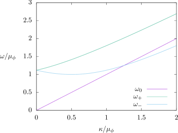
Figure 1: Plot of the dispersion relations of the Majorana modes in the case of negligible $M$, given in Eq. (5.47). For the plot we taken $|m|^{2}\sim\mu^{2}_{\phi}$. For reference, the plot of the dispersion relation $\omega_{0}=\kappa$ is superimposed.

$|m|\ll M$ limit.

In this limit, the $d$ term in Eq. (5.39) can be approximated by

$$d=4M^{2}|m|^{2}+\mu^{2}_{\phi}\kappa^{2}+\mu^{2}_{\phi}M^{2}\,,$$ (5.43)

so that the dispersion relations reduce to

$$\omega^{2}_{\pm}(\kappa)=\kappa^{2}+M^{2}+|m|^{2}+\frac{1}{4}\mu^{2}_{\phi}\pm 2\sqrt{M^{2}|m|^{2}+\frac{1}{4}\mu^{2}_{\phi}\kappa^{2}+\frac{1}{4}\mu^{2}_{\phi}M^{2}}\,.$$ (5.44)

Further, taking the $\kappa\rightarrow 0$ limit,

$$\omega^{2}_{\pm}(0)=\left(M\pm\sqrt{|m|^{2}+\frac{1}{4}\mu^{2}_{\phi}}\right)^{2}\,,$$ (5.45)

which can be interpreted as the effective masses of the Majorana modes, in the $|m|\ll M$ limit. But again, the $\kappa$ dependence of the dispersion relation is different than the one given in Eqs. (5.41) and (5.42). In the case that $|m|$ can be neglected relative to $\mu_{\phi}$ (for example, if $\mu_{\phi}$ is sufficiently close to $m_{\phi}$), then Eq. (5.44) can be approximated by

$$\omega_{\pm}(\kappa)=\sqrt{\kappa^{2}+M^{2}}\pm\frac{1}{2}\mu_{\phi}\,,$$ (5.46)

which resemble the dispersion relation of a neutrino propagating in a matter background with a Wolfenstein-like potential $V_{\text{eff}}=\frac{1}{2}\mu_{\phi}$.

Small $M$ limit.

For sufficently small values of $M$, the dispersion relations are approximated by

$$\omega^{2}_{\pm}=\kappa^{2}+|m|^{2}+\frac{1}{4}\mu^{2}_{\phi}\pm\mu_{\phi}\kappa\,.$$ (5.47)

Therefore, the two modes have the same efective mass

$$\omega(0)=\sqrt{|m|^{2}+\frac{1}{4}\mu^{2}_{\phi}}\,,$$ (5.48)

but different dispersion relations away from $\kappa=0$. A plot of Eq. (5.47) is shown in Fig. 1.

6 Conclusions and outlook

In previous works we have carried out a systematic calculation of the neutrino dispersion relation, as well as the damping and decoherence effects, when the neutrino propagates in a thermal background of fermions and scalars, with a Yukawa-type interaction between the neutrino and the background particles [see Ref. [12] and references therein].

As a complement of that work, the motivation of the present work is to determine the corresponding quantities for the case in which the scalar background consists of a Bose-Einstein condensate. To this end, here we have proposed an efficient and consistent method to treat the propagation of generic fermions in the background of BE condensate. With an outlook to possible application in other contexts, we have illustrated and implemented the method in a general way and not tied to any specific application. In the present work we have focused exclusively on the calculation of the dispersion relations. To model the propagation of the fermions in such an environment, we assumed some simple Yukawa-type interactions between the fermions and the scalar.

As mentioned in the Introduction, the method we use to treat the BE condensate has been discussed by various authors[23, 24, 25]. In Section 2 we reviewed those aspects and details of the method that are relevant for our purposes. In the following three sections we presented the extension we propose of that method to treat the propagation of fermions in the BE condensate, in the context of three generic, but specific, models of the fermion-scalar interaction. Specifically in Section 3 we considered two massless chiral fermions, $f_{L}$ and $f_{R}$, with a coupling to the scalar particle $\phi$ of the form $\bar{f}_{R}f_{L}\phi$ (Model I). In Section 4 we considered a massless chiral fermion $f_{L}$ with coupling $\bar{f}^{c}_{R}f_{L}\phi$ (Model II). Finally in Section 5 we considered one massive Dirac fermion $f$ with a coupling $\bar{f}^{c}f\phi$ (Model III).

In each case we determined the fermion modes and corresponding dispersion relations and pointed out some of their particular characteristics. For example, as a result of the symmetry breaking the propagating mode is a Dirac fermion and a Majorana fermion in Models I and II, respectively. In Model III the symmetry breaking produces two non-degenerate Majorana modes of what otherwise would form a Dirac fermion field in the unbroken phase. In the latter case, various particular features of the dispersion relations of the Majorana modes were illustrated by considering particular limiting cases of the parameters of the model. For example, one interesting observation is that, while in general the two Majorana modes have different effective masses (the value of the dispersion relation at zero momentum), in some limits the two modes have the same effective mass although the dispersion relations at non-zero momentum are different.

The method we propose for the propagation of fermions in a BE condensate has never being used before, and can be applicable in various contexts, for example neutrino physics, condensed or nuclear matter systems and heavy-ion collisions. In addition, the work sets the ground for considering the case of various fermion flavors, as would be required for the aplication to neutrinos, or the corrections to the dispersion relations due to the thermal effects of the background excitations, that could be required for particular applications.

The work of S. S. is partially supported by DGAPA-UNAM (Mexico) PAPIIT project No. IN103522.

Appendix A Transformation of the chemical potential

Here we show and state precisely the result we invoke in Section 2 regarding the use of the $\phi^{\prime}$ field (with its corresponding Lagrangian $L^{(\phi^{\prime})}$) in the thermal field theory calculations while setting $\mu_{\phi}=0$ in the partition function. Moreover, as will become evident, the result also holds for any other field, not just for the $\phi$ field, that is transformed in a similar way as we have done for the fermions.

We denote by $Q_{A}$ the set of conserved charges associated with the symmetries of the Lagrangian, which are such that

$$[Q_{A},\phi]=-q_{A}\phi\,.$$ (A.1)

The partition function is given by

$$Z=e^{-\beta H+Q}\,,$$ (A.2)

where

$$Q=\sum_{A}\alpha_{A}Q_{A}\,,$$ (A.3)

and the chemical potential of $\phi$ is given by

$$\mu_{\phi}=\frac{\alpha_{\phi}}{\beta}\,,$$ (A.4)

where

$$\alpha_{\phi}\equiv\sum_{A}\alpha_{A}q_{A}\,.$$ (A.5)

From Eq. (A.1) we have

$$[Q,\phi]=-\alpha_{\phi}\phi\,.$$ (A.6)

The statement we now show is this: if instead of carrying the calculations with the $\phi$ field and its original Lagrangian $L$ and corresponding Hamiltonian $H$, we use the $\phi^{\prime}$ field, with the transformed Lagrangian $L^{\prime}$ and corresponding Hamiltonian $H^{\prime}$, then the partition function becomes

$$Z=e^{-\beta H^{\prime}}\,,$$ (A.7)

when it is expressed in terms of the prime field. As already mentioned, a somewhat exhaustive discussion of this point is given in Ref. [23]. A simple way to understand this result is the following.

The evolution equation for $\phi$ is given by

$$i\partial_{t}\phi=-[H,\phi]\,,$$ (A.8)

where $H$ is the Hamiltonian corresponding to the Lagrangian $L$. If now calculate the time derivative of $\phi^{\prime}\equiv e^{i\mu_{\phi}t}\phi$ we get

$$\partial_{t}\phi^{\prime} = i\mu_{\phi}\phi^{\prime}+e^{i\mu_{\phi}t}\partial_{t}\phi$$ (A.9)

$$= i\mu_{\phi}\phi^{\prime}+e^{i\mu_{\phi}t}i[H,\phi]$$

$$= i\mu_{\phi}\phi^{\prime}+i[H,\phi^{\prime}]$$

$$= -\frac{i}{\beta}[Q,\phi^{\prime}]+i[H,\phi^{\prime}]$$

$$= i[H-\frac{1}{\beta}Q,\phi^{\prime}]\,,$$

or

$$i\partial_{t}\phi^{\prime}=-[H-\frac{1}{\beta}Q,\phi^{\prime}]\,.$$ (A.10)

In other words, the Hamiltonian that governs the evolution of $\phi^{\prime}$ is $H-\frac{1}{\beta}Q$, or equivalently the two Hamiltonians are related by

$$H^{\prime}=H-\frac{1}{\beta}Q\,.$$ (A.11)

Therefore, when we express the partition function in terms of the field $\phi^{\prime}$,

$$Z=e^{-\beta H+Q}=e^{-\beta H^{\prime}}\,.$$ (A.12)

That is, in the calculations using $\phi^{\prime}$ we use the partition function with its Hamiltonian $H^{\prime}$ and zero chemical potential.

The reason we emphasize here the operator proof of Eq. (A.11), is because in this way it is applicable to any field (e.g., a fermion field), not involving Lagrangian dynamics arguments, and therefore the result shown above holds for any field and not a scalar field. On the other hand, the Lagrangian formulation we carried out in Section 2 is the most efficient way to do the dynamics of the $\phi^{\prime}$, which makes very straightforward to solve the evolution equations, rather than starting with the Hamilton equation, to find the dispersion relations, propagators and wave functions of the propagating modes.

Appendix B Scalar modes of the BE condensate

In this appendix we complete the discussion of the model presented in Section 2 with regard to the $\phi_{1,2}$ excitation modes of the BE condensate. To simplify the notation, here we omit the subscript in the chemical potential, mass and quartic coupling of the $\phi$ and denote them by simply $\mu,m,\lambda$ (without the $\phi$ subscript), respectively.

B.1 Lagrangian for the scalar modes

As already mentioned in Section 2, the starting point is to substitute Eqs. (2.15) and (2.18) in Eq. (2.12) to obtain the Lagrangian for the scalar excitations $\phi_{1,2}$. Doing piece by piece,

$$(\partial^{\mu}\phi^{\prime})^{\ast}(\partial_{\mu}\phi^{\prime}) = \frac{1}{2}\left[(\partial^{\mu}\phi_{1})^{2}+(\partial^{\mu}\phi_{2})^{2}\right]\,,$$

$$i[\phi^{\prime\,\ast}(v\cdot\partial\phi^{\prime})-(v\cdot\partial\phi^{\prime})^{\ast}\phi^{\prime}] = 2\mbox{Re}\left(i\phi^{\ast}v\cdot\partial\phi\right)$$ (B.1)

$$= \phi_{2}v\cdot\partial(\phi_{1}+\phi_{0})-(\phi_{1}+\phi_{0})v\cdot\partial\phi_{2}$$

$$= \phi_{2}v\cdot\partial\phi_{1}-\phi_{1}v\cdot\partial\phi_{2}-\phi_{0}v\cdot\partial\phi_{2}\,.$$

The last term is a total derivative and therefore does not contribute to the action or the equations of motion and can be dropped. Finally,

$$U(\phi^{\prime}) = -\frac{1}{2}(\mu^{2}-m^{2})[(\phi_{0}+\phi_{1})^{2}+\phi^{2}_{2}]+\frac{1}{4}\lambda[(\phi_{0}+\phi_{1})^{2}+\phi^{2}_{2}]^{2}$$ (B.2)

$$= U_{0}+U_{1}+U_{2}+U_{3}+U_{4}\,,$$

where $U_{0}$ has been defined in Eq. (2.17), and

$$U_{1} = \frac{\partial U_{0}}{\partial\phi_{0}}\phi_{1}\,,$$

$$U_{2} = -\frac{1}{2}(\mu^{2}-m^{2})[\phi^{2}_{1}+\phi^{2}_{2}]+\frac{1}{2}\lambda\phi^{2}_{0}\phi^{2}_{2}+\frac{3}{2}\lambda\phi^{2}_{0}\phi^{2}_{1}\,,$$

$$U_{3} = \lambda\phi_{0}(\phi^{3}_{1}+\phi_{1}\phi^{2}_{2})\,,$$

$$U_{4} = \frac{\lambda}{4}(\phi^{4}_{1}+\phi^{4}_{2}+2\phi^{2}_{1}\phi^{2}_{2})\,.$$ (B.3)

The terms $U_{3,4}$ give the self-interactions between $\phi_{1,2}$ which we are not interested in at the moment, $U_{0}$ is an irrelevant constant, and $U_{1}=0$ when Eq. (2.18) is used. The quadratic part, using Eq. (2.18) is

$$U_{2}=\frac{1}{2}m^{2}_{1}\phi^{2}_{1}+\frac{1}{2}m^{2}_{2}\phi^{2}_{2}\,,$$ (B.4)

where

$$m^{2}_{1} = -(\mu^{2}-m^{2})+3\lambda\phi^{2}_{0}$$

$$= 2(\mu^{2}-m^{2})\,,$$

$$m^{2}_{2} = -(\mu^{2}-m^{2})+\lambda\phi^{2}_{0}$$ (B.5)

$$= 0\,.$$

In the second line in each equation we have used Eq. (2.18). Therefore, the quadratic part of the $\phi_{1,2}$ Lagrangian is

$$L^{(2)}_{\phi}=\frac{1}{2}\left[(\partial^{\mu}\phi_{1})^{2}+(\partial^{\mu}\phi_{2})^{2}\right]+\phi_{2}v\cdot\partial\phi_{1}-\phi_{1}v\cdot\partial\phi_{2}-\frac{1}{2}m^{2}_{1}\phi^{2}_{1}\,.$$ (B.6)

Thus $\phi_{1}$ and $\phi_{2}$ are mixed by the $v^{\mu}$ term. The next step is to find the propagator matrix of the $\phi_{1,2}$ complex and determine the modes that have a definite dispersion relation.

B.2 Dispersion relations for the scalar modes

Using matrix notation,

$$\hat{\phi}=\left(\begin{array}[]{l}\phi_{1}\\ \phi_{2}\end{array}\right)\,,$$ (B.7)

the Lagrangian, in momentum space, is

$$L^{(2)}_{\phi}(k)=\frac{1}{2}\hat{\phi}^{\ast}(k)\Delta^{-1}_{\phi}(k)\hat{\phi}(k)\,,$$ (B.8)

where

$$\Delta^{-1}_{\phi}(k)=\left(\begin{array}[]{ll}k^{2}-m^{2}_{1}&2iv\cdot k\\ -2iv\cdot k&k^{2}\end{array}\right)\,.$$ (B.9)

The classical equations of motion are then

$$\Delta^{-1}_{\phi}(k)\hat{\phi}=0\,.$$ (B.10)

The dispersion relations of the eigenmodes are given by the solutions of

$$D=0\,,$$ (B.11)

where $D$ is the determinant of $\Delta^{-1}_{\phi}$,

$$D\equiv k^{2}(k^{2}-m^{2}_{1})-4(v\cdot k)^{2}\,,$$ (B.12)

or,

$$D=(\omega^{2}-\kappa^{2})(\omega^{2}-\kappa^{2}-m^{2}_{1})-\alpha^{2}\omega^{2}\,,$$ (B.13)

where we have defined

$$\alpha=2\mu\,.$$ (B.14)

The dispersion relations are determined by solving

$$(\omega^{2}-\kappa^{2})(\omega^{2}-\kappa^{2}-m^{2}_{1})-\alpha^{2}\omega^{2}=0\,,$$ (B.15)

which we write in the form

$$(\omega^{2}-\kappa^{2})(\omega^{2}-\kappa^{2}-m^{2}_{1})-\alpha^{2}(\omega^{2}-\kappa^{2})-\alpha^{2}\kappa^{2} = 0\,,$$

$$(\omega^{2}-\kappa^{2})^{2}-(\omega^{2}-\kappa^{2})(m^{2}_{1}+\alpha^{2})-\alpha^{2}\kappa^{2} = 0\,.$$ (B.16)

This is a quadratic equation for $(\omega^{2}-\kappa^{2})$ with solutions

$$\omega^{2}_{\pm}(\kappa)=\kappa^{2}+\frac{1}{2}(m^{2}_{1}+\alpha^{2})\pm\sqrt{\frac{1}{4}(m^{2}_{1}+\alpha^{2})^{2}+\alpha^{2}\kappa^{2}}\,,$$ (B.17)

and obviously,

$$D=(\omega^{2}-\omega^{2}_{+})(\omega^{2}-\omega^{2}_{-})\,.$$ (B.18)

Thus, the masses of the propagating modes are

$$m^{2}_{+} = m^{2}_{1}+\alpha^{2}\,,$$

$$m^{2}_{-} = 0\,.$$ (B.19)

The zero mass mode is the realization of the Goldstone mode associated with the breaking of the global $U(1)$ symmetry.

The corresponding eigenvectors satisfy

$$\left.\Delta^{-1}_{\phi}(k)\right|_{\omega=\omega_{s}}\hat{\phi}_{s}(\kappa)=0\,,$$ (B.20)

where $s=\pm$. Writing

$$\hat{\phi}_{s}(\kappa)=\left(\begin{array}[]{l}a_{s}\\ b_{s}\end{array}\right)\,,$$ (B.21)

the equations for the components are

$$(\omega^{2}_{s}-\kappa^{2}-m^{2}_{1})a_{s}+i\alpha\omega_{s}b_{s} = 0\,,$$

$$-i\alpha\omega_{s}a_{s}+(\omega^{2}_{s}-\kappa^{2})b_{s} = 0\,.$$ (B.22)

We write the solutions in the form

$$\hat{\phi}_{+}(\kappa) = \frac{1}{\sqrt{N_{+}}}\left(\begin{array}[]{l}\omega^{2}_{+}-\kappa^{2}\\ i\alpha\omega_{+}\end{array}\right)\,,$$ (B.25)

$$\hat{\phi}_{-}(\kappa) = \frac{1}{\sqrt{N_{-}}}\left(\begin{array}[]{l}-i\alpha\omega_{-}\\ \omega^{2}_{-}-\kappa^{2}-m^{2}_{1}\end{array}\right)\,.$$ (B.28)

The normalization factors $N_{\pm}$ are determined by requiring that the one-particle contribution to the propagator from the eigenmodes coincide with the form of the propagator near the dispersion relations ($\omega\rightarrow\omega_{s}$). The procedure is the following. Instead of expressing $\hat{\phi}$ in terms of the $1,2$ modes,

$$\hat{\phi}(k)=\left(\begin{array}[]{c}\phi_{1}(k)\\ \phi_{2}(k)\end{array}\right)\,,$$ (B.29)

it is expressed in terms of the modes that have a definite dispersion relation,

$$\hat{\phi}(k)=\sum_{s=\pm}c_{s}(k)\hat{\phi}_{s}(\kappa)\,,$$ (B.30)

where the $\phi_{s}$ are the eigenvectors found above. The free-field $\hat{\phi}(x)$ is then expanded in the usual form,

$$\hat{\phi}(x)=\sum_{s=\pm}\int\frac{d^{3}\kappa}{(2\pi)^{3}2\omega_{s}(\kappa)}\left[e^{-ik_{s}\cdot x}a_{s}(\vec{\kappa})\hat{\phi}_{s}(\kappa)+e^{ik_{s}\cdot x}a^{\ast}_{s}(\vec{\kappa})\hat{\phi}^{\ast}_{s}(\kappa)\right]\,,$$ (B.31)

with

$$[a_{s}(\vec{\kappa}),a^{\ast}_{s}(\vec{\kappa}^{\prime})]=(2\pi)^{3}2\omega_{s}(\kappa)\delta(\vec{\kappa}-\vec{\kappa}^{\prime})\,,$$ (B.32)

and

$$k^{\mu}_{s}=(\omega_{s},\vec{\kappa})\,.$$ (B.33)

The one-particle contribution to the propagator from a given mode is then

$$\left.\Delta_{\phi}\right|_{\text{one-particle},s}=\frac{\hat{\phi}_{s}\hat{\phi}^{\dagger}_{s}}{2\omega_{s}(\omega-\omega_{s})}\,.$$ (B.34)

For reference and example, we give explicitly the formula for $s=+$,

$$\hat{\phi}_{+}\hat{\phi}^{\dagger}_{+}=\frac{1}{N_{+}}\left(\begin{array}[]{ll}(\omega^{2}_{+}-\kappa^{2})(\omega^{2}_{+}-\kappa^{2})&(\omega^{2}_{+}-\kappa^{2})(-i\alpha\omega_{+})\\ i\alpha\omega_{+}(\omega^{2}_{+}-\kappa^{2})&(i\alpha\omega_{+})(-i\alpha\omega_{+})\end{array}\right)\,.$$ (B.35)

On the other hand, by inverting Eq. (B.9), we obtain the propagator of the $\phi_{1,2}$ complex

$$\Delta_{\phi}(k)=\frac{1}{D}\left(\begin{array}[]{ll}k^{2}&-i\alpha\omega\\ i\alpha\omega&k^{2}-m^{2}_{1}\end{array}\right)\,.$$ (B.36)

where $D$ is given in Eq. (B.13). The propagator has poles at the dispersion relations given in Eq. (B.17). Using Eq. (B.18), near the $\omega=\omega_{+}$ pole, Eq. (B.36) gives

$$\left.\Delta_{\phi}(k)\right|_{\omega\rightarrow\omega_{+}}=\frac{1}{2\omega_{+}(\omega-\omega_{+})(\omega^{2}_{+}-\omega^{2}_{-})}\left(\begin{array}[]{ll}\omega^{2}_{+}-\kappa^{2}&-i\alpha\omega_{+}\\ i\alpha\omega_{+}&\omega^{2}_{+}-\kappa^{2}-m^{2}_{1}\end{array}\right)\,.$$ (B.39)

The normalization factor $N_{+}$ is determined by requiring that

$$\left.\Delta_{\phi}\right|_{\omega\rightarrow\omega_{+}}=\left.\Delta_{\phi}\right|_{\text{one-particle},+}\,.$$ (B.40)

Comparing Eqs. (B.34) and (B.39), the normalization factor is then determined by requiring that

$$\hat{\phi}_{+}\hat{\phi}^{\dagger}_{+}=\frac{1}{\omega^{2}_{+}-\omega^{2}_{-}}\left(\begin{array}[]{ll}\omega^{2}_{+}-\kappa^{2}&-i\alpha\omega_{+}\\ i\alpha\omega_{+}&\omega^{2}_{+}-\kappa^{2}-m^{2}_{1}\end{array}\right)\,,$$ (B.41)

and using Eq. (B.35) (and remembering Eq. (B.15), for the 22 element) we then obtain the wave function renormalization factor

$$\frac{1}{N_{+}}=\frac{1}{\omega^{2}_{+}-\omega^{2}_{-}}\frac{1}{\omega^{2}_{+}-\kappa^{2}}\,.$$ (B.42)

Applying similar arguments to $N_{-}$,

$$\frac{1}{N_{-}}=\frac{1}{\omega^{2}_{+}-\omega^{2}_{-}}\frac{1}{\kappa^{2}+m^{2}_{1}-\omega^{2}_{-}}\,.$$ (B.43)

References

• [1] See for example, H. Duan, G. M. Fuller and Y. Z. Qian, Collective Neutrino Oscillations, Ann. Rev. Nucl. Part. Sci.  60, 569 (2010) [arXiv:1001.2799 [hep-ph]], and references therein
• [2] S. Chakraborty, R. Hansen, I. Izaguirre and G. Raffelt, Collective neutrino flavor conversion: Recent developments, Nucl. Phys. B 908, 366 (2016) [arXiv:1602.02766].
• [3] Y. Y. Y. Wong, Analytical treatment of neutrino asymmetry equilibration from flavor oscillations in the early universe, Phys. Rev. D 66, 025015 (2002) [arXiv:hep-ph/0203180].
• [4] G. Mangano, G. Miele, S. Pastor, T. Pinto, O. Pisanti and P. D. Serpico, Effects of non-standard neutrino-electron interactions on relic neutrino decoupling, Nucl. Phys. B 756, 100 (2006) [arXiv:hep-ph/0607267].
• [5] K. S. Babu, Garv Chauhan, P. S. Bhupal Dev, Neutrino Non-Standard Interactions via Light Scalars in the Earth, Sun, Supernovae and the Early Universe, Phys. Rev. D 101, 095029 (2020) [arXiv:1912.13488].
• [6] G. Mangano, A. Melchiorri, P. Serra, A. Cooray and M. Kamionkowski, Cosmological bounds on dark matter-neutrino interactions, Phys. Rev. D 74, 043517 (2006) [arXiv:astro-ph/0606190].
• [7] T. Binder, L. Covi, A. Kamada, H. Murayama, T. Takahashi and N. Yoshida, Matter Power Spectrum in Hidden Neutrino Interacting Dark Matter Models: A Closer Look at the Collision Term, JCAP 1611, 043 (2016) [arXiv:1602.07624].
• [8] R. Primulando and P. Uttayarat, Dark Matter-Neutrino Interaction in Light of Collider and Neutrino Telescope Data, JHEP 1806, 026 (2018) [arXiv:1710.08567].
• [9] A. Olivares-Del Campo, C. Bœhm, S. Palomares-Ruiz and S. Pascoli, Dark matter-neutrino interactions through the lens of their cosmological implications, Phys. Rev. D 97, 075039 (2018) [arXiv:1711.05283].
• [10] T. Franarin, M. Fairbairn and J. H. Davis, JUNO Sensitivity to Resonant Absorption of Galactic Supernova Neutrinos by Dark Matter, [arXiv:1806.05015].
• [11] S. Pandey, S. Karmakar and S. Rakshit, Interactions of Astrophysical Neutrinos with Dark Matter: A model building perspective, JHEP 1901, 095 (2019) [Erratum: JHEP 11, 215 (2021)] [arXiv:1810.04203]
• [12] Jose F Nieves and Sarira Sahu, Neutrino effective potential in a fermion and scalar background in the resonace region, Phys. Rev. D 105, 095022 (2022), [arxiv: 2201.04661]
• [13] See for example, N. P. Landsman and C. G. van Weert, Real and Imaginary Time Field Theory at Finite Temperature and Density, Phys. Rept.  145, 141 (1987); J. I. Kapusta, Finite Temperature Field Theory, (Cambridge University Press,Cambridge, 1989); A. K. Das, Finite Temperature Field Theory, (World Scientific Singapore, 1997); M. L. Bellac, Thermal Field Theory, (Cambridge University Press, Cambridge, 2011).
• [14] Raghuveer Garani, Michel H.G. Tytgat, Jérôme Vandecasteele, Condensed dark matter with a Yukawa interaction, Phys. Rev. D 106, 116003 (2022) [arxiv:2207.06928]
• [15] Kay Kirkpatrick and Anthony E. Mirasola and Chanda Prescod-Weinstein Analysis of Bose-Einstein condensation times for self-interacting scalar dark matter, Phys. Rev. D 106, 043512 (2022) [arxiv: 2110.08921]
• [16] C. G. Boehmer, T. Harko, Can dark matter be a Bose-Einstein condensate?, JCAP 0706:025 (2007) [arxiv:0705.4158]
• [17] Maria Crǎciun, Tiberiu Harko, Testing Bose-Einstein Condensate dark matter models with the SPARC galactic rotation curves data, European Physical Journal C, 80, 735 (2020) [arxiv:2007.12222]
• [18] Gordan Baym, Christopher Pethick, Neutron Stars, Annu. Rev. Nucl. Sci. 25, 27 (1975).
• [19] Vesteinn Thorsson, Madappa Prakash, J. M. Lattimer Composition, structure and evolution of neutron stars with kaon condensates, Nucl. Phys. A, 572, 693 (1994).
• [20] A. Schmitt, Dense Matter in Compact Stars, A Pedagogical Introduction, Lect. Notes Phys. 811 (Springer, Berlin Heidelberg 2010) [DOI 10.1007/978-3-642-12]
• [21] G. Q. Li, C. -H. Lee, G. E. Brown, Kaons in dense matter, kaon productionin heavy-ion collisions, and kaon condensation in neutron stars, Nucl. Phys. A, 625, 372 (1997).
• [22] The terminology of a “pseudo-Dirac fermion” is borrowed from the pseudo-Dirac neutrino model: L. Wolfenstein, Nucl. Phys. B186, 147 (1981); S. T. Petcov, Phys. Lett. 110B, 245 (1982).
• [23] H. Arthur Weldon, Chemical potentials in real-time thermal field theory, Phys. Rev. D 76, 125029 (2007)
• [24] Antonio Filippi, Inclusion of Chemical Potential for Scalar Fields, Imperial/TP/96-97/37 [arxiv:hep-ph/9703323v1]
• [25] See Appendix A in Ref. [20],
• [26] Alan H. Guth, Mark P. Hertzberg, C. Prescod-Weinstein, Do Dark Matter Axions Form a Condensate with Long-Range Correlation?, Phys. Rev. D 92, 103513 (2015), [arxiv:1412.5930]