Rethink long-tailed recognition with Vision transformers

Abstract

In the real world, data tends to follow long-tailed distributions w.r.t. class or attribution, motivating the challenging Long-Tailed Recognition (LTR) problem. In this paper, we revisit recent LTR methods with promising Vision Transformers (ViT). We figure out that 1) ViT is hard to train with long-tailed data. 2) ViT learns generalized features in an unsupervised manner, like mask generative training, either on long-tailed or balanced datasets. Hence, we propose to adopt unsupervised learning to utilize long-tailed data. Furthermore, we propose the Predictive Distribution Calibration (PDC) as a novel metric for LTR, where the model tends to simply classify inputs into common classes. Our PDC can measure the model calibration of predictive preferences quantitatively. On this basis, we find many LTR approaches alleviate it slightly, despite the accuracy improvement. Extensive experiments on benchmark datasets validate that PDC reflects the model’s predictive preference precisely, which is consistent with the visualization.

Index Terms—  metric, long-tailed learning, vision transformers, representation learning, imbalanced data.

1 Introduction

With rapid advances in visual classification, deep models tend to depend on balanced large-scale datasets more seriously [1, 2]. However, the number of instances in real-world data usually follows a Long-Tailed (LT) distribution w.r.t. class. Many tail classes are associated with limited samples, while a few head categories occupy most of the instances [3, 4, 5, 6]. The model supervised by long-tailed data tends to bias toward the head classes and ignore the tail ones. The tail data paucity makes the model hard to train with satisfying generalization. It is still a challenging task to overcome Long Tailed Recognition (LTR) and utilize real-world data effectively.

Recent literature mainly adopt two approaches to tackle LT data, i.e., feature re-sampling and class-wise re-weighting. The re-sampling methods balanced select the training data by over-sampling the tail or under-sampling the head. Some effective proposals replenish the tail samples via generation or optimization with the help of head instances[7, 8]. The re-weighting ones punish different categories with data number relevant weight or logit bias[9, 10]. Although the aforementioned methods have greatly mitigated the LT problem, the conclusions hold on the ResNet-based backbones [11, 12].

In recent years, many transformer-based backbones [13] have surpassed the performance of CNN. DeiT[14] proposes an effective receipt to train ViT with limited data, and MAE[15] adopts a masked autoencoder to pre-train the ViT. However, there is limited research on how ViTs perform on LTR. Motivated by this, we rethink the previous LT works with ViT. We figure out that it is hard to train ViTs with long-tailed data while the unsupervised pretraining manner ameliorates it by a large margin. The unsupervised pretraining ViTs will learn meaningful feature (c.f. Figure 2) and generalize well on downstream tasks (c.f. Table 2), either on long-tailed or balanced datasets.

Numerous studies have demonstrated that the model supervised by the LT dataset will inevitably exhibit prediction bias to the head[5, 16, 17, 18]. The predictor will simply classify the inquiry image to the head to attain a low misclassification error. The previous metrics, like accuracy on the validation dataset, are difficult to evaluate the model’s predictive preference directly. The same accuracy may come at the cost of a different number of predictions (c.f. Figure 1). Although some works show models’ prediction distribution by visualization qualitatively[5, 11, 19], a metric is required to evaluate it quantitatively. In this paper, we propose Prediction Distribution Calibration (PDC) to fill this gap. Specifically, if we view the prediction number and target instance number of each class as probability distributions, we can measure the distance between the two probability distributions. Considering the imbalance degree of training samples, we take the training label into account as well. To summarize, our main contributions are:

1) We figure out that it is difficult to train ViT with long-tailed data, which can be tackled with unsupervised pretraining.

2) We propose PDC to provide a quantitative view to measure how the proposal ameliorates the model predictive preference.

3) We conduct extensive experiments to analyze LTR proposals’ performance on ViT with our proposed PDC, which will accurately indicate the model’s predictive bias and is consistent with the visualization results.

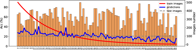
Fig. 1: Visualization of ViT-B on CIFAT100-LT (IF=100). Acc trap: the accuracy can not reflect predictive bias. A class can obtain on par accuracy with another one with much more predictions. Take class 0 and 99 for an illustration.

2 The proposed approach

2.1 Long Tail Recognition

Given an $C$-classes labeled dataset containing $N$ training instances, $\mathbf{D}=\left\{\left(x_{1},y_{1}\right),\left(x_{2},y_{2}\right),\ldots,\left(x_{n},y_{n}\right)\right\}$, where $y_{i}\in\mathcal{C}=\{1,...,C\}$ and the distribution is $\mathbb{P}(\mathbf{x},\mathbf{y})$. In this paper, we define a base classification model as ${\mathcal{M}_{\theta}}$, which is parameterized by $\theta$. For each input image $x$, the output logits as ${\mathbf{z}_{\theta}(x)=\mathcal{M}(x|\theta)}=\{z_{1},...,z_{c}\}$. The goal is to optimize the parameters $\theta$ to get the best estimation of $\mathbb{P}(\mathbf{x},\mathbf{y})$. Generally, one adopts softmax function to map the output ${\mathcal{M}_{(}x|\theta)}$ as the conditional probability:

$$p\left(\mathbf{y}\mid\mathbf{x};\theta\right)=\frac{e^{\mathcal{M}(\mathbf{x}\mid\theta)_{\mathbf{y}}}}{\sum_{i}e^{\mathcal{M}(\mathbf{x}\mid\theta,\phi)_{\mathbf{y}_{i}}}}$$ (1)

We get the posterior estimates $\mathbb{P}(y|x):=p\left(\mathbf{y}|\mathbf{x};\theta\right)$ by maximum likelihood $\mathbb{P}(x|y)$ estimation, which is represented by model parameters $\theta$. In LTR, we train the model with long-tailed distributed training data $\mathbb{P}_{s}(x,y)$ while evaluating it with uniform ones $\mathbb{P}_{t}(x,y)$. The label prior distribution $\mathbb{P}_{s}(y)$ will be different for each class while keeping consistent in the test dataset, i.e., $\mathbb{P}_{t}(y):=1/C$. For a tail class $i$, $\mathbb{P}_{s}(y_{i})\ll\mathbb{P}_{t}(y_{i})$. According to the Bayesian Theory, the posterior is proportional to the prior times the likelihood. Considering the same likelihood, i.e., $\mathbb{P}_{s}(x|y)=\mathbb{P}_{t}(x|y)$, we have the posterior on the target dataset:

$$\mathbb{P}_{t}(y_{i}|x)=\mathbb{P}(x|y_{i})\cdot\mathbb{P}_{s}(y_{i})/\mathbb{P}_{t}(y_{i})$$ (2)

With the Eq.2 and balanced target distribution $\mathbb{P}_{t}(y):=1/C$, we have $\mathbb{P}_{t}(y_{i}|x)\propto\mathbb{P}_{s}(y_{i})$. Therefore, models tend to predict a query image into head classes to satisfy the train label distribution $\mathbb{P}_{s}(y_{i})$, which is called predictive bias. Such a mismatch makes the generalization in LTR extremely challenging, and the traditional metrics, e.g., mean accuracy on the training dataset, exacerbates biased estimation when evaluating models on the balanced test set.

2.2 Vision Transforms

ViT reshapes a image $x\in\mathbb{R}^{H\times W\times C}$ into a sequence (length $L=H\times W/P^{2}$) of flattened 2D patches $x_{P}\in\mathbb{R}^{L\times(P^{2}\cdot C)}$, where $H\times W$ are the resolution of $x$, $C$ is channels, $P$ is the patch resolution. Although ViTs perform well on numerous visual tasks, we figure out that it is hard to train ViTs with long-tailed data, and the performance is unsatisfactory. Recent work trains ViTs without label supervision by the encoder ($\mathcal{E}$) decoder ($\mathcal{D}$) architecture and random mask $\mathbf{M}$:

$$\hat{\mathbf{x}}=\mathcal{D}\left(\mathcal{E}(\mathbf{M}\odot\mathbf{x})\right)$$ (3)

Table 1: Performance on CIFAR100-LT. Acc@R: Top1 accuracy with ResNet32. Acc@V: Top1 accuracy with ViT-B.

Imbalance	10			50			100			var.
Method	Acc@R	Acc@V	PDC$\downarrow$	Acc@R	Acc@V	PDC$\downarrow$	Acc@R	Acc@V	PDC$\downarrow$
CE	55.70	66.02	0.34	43.90	54.78	0.62	38.30	50.59	0.64	0.03
BCE [20]	-	64.63	0.46	-	50.65	1.31	-	45.50	2.25	0.80
CB [3]	57.99	66.30	0.06	45.32	56.18	0.08	45.32	50.63	0.13	0.00
LDAM [21]	56.91	63.99	0.47	45.00	54.53	0.61	39.60	50.39	0.82	0.03
MiSLAS [11]	63.20	66.65	0.26	52.30	55.90	0.56	47.00	50.62	0.94	0.12
LADE [10]	61.70	68.32	0.07	50.50	60.03	0.10	45.40	57.25	0.10	0.00
IB [12]	57.13	65.12	0.06	46.22	43.78	1.09	42.14	42.30	0.46	0.27
BalCE [9]	63.00	68.11	0.04	49.76	60.67	0.04	50.80	56.86	0.05	0.00

We pinpoint that the ViTs will learn generalized feature extraction by Eq.3, either on long-tailed or balanced datasets. Such an observation inspires us to adopt it as a strong baseline to evaluate the performance with ViTs.

2.3 Predictive Distribution Calibration

In LTR, recent works try to compensate for the mismatch of $\mathbb{P}_{s}(y)$ and $\mathbb{P}_{t}(y)$, which is described in section 2.1. However, they all adopt the Top1-accuracy to evaluate their proposals, which fails to show whether the mismatch is fixed. To fill the gap and measure it intuitively, we propose the Predictive Distribution Calibration (PDC) to quantitative analyze the model’s predictive bias.

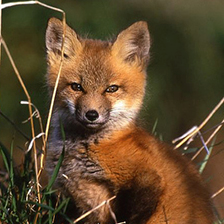
(a) Input

(b) Masked

(c) Reco.+LT

(d) Reco.+BAL

(e) Reco.+LT+U

(f) Reco.+BAL+U

Fig. 2: Reconstruction visualization of MAE. LT: pretrain with long-tailed data. BAL: pretrain with balanced data. LT and BAL have the same total instances. U: add unmasked patch. ViTs pretrained on both LT and BAL learn meaningful features.

Step 1: Here, we view the prediction number w.r.t. class as the predictive distribution $\hat{\mathbb{P}}_{t}(y)$. Considering the balanced label distribution $\mathbb{P}_{t}(y)$, we can calculate the distance between the above two distributions. Considering to measure this distance via Kullback-Leibler divergence (KL), we have:

$$D(\mathbb{P}_{t},\hat{\mathbb{P}}_{t})=\frac{1}{C}\sum_{y_{i}\in\mathcal{C}}\mathbb{P}_{t}(y_{i})\cdot\left[\log\mathbb{P}_{t}(y_{i})-\log\hat{\mathbb{P}}_{t}(y_{i})\right]\!$$ (4)

Step 2: Generally, the larger gap between $\mathbb{P}_{s}(y)$ and $\mathbb{P}_{t}(y)$, the more difficult to overcome the model predictive bias. To eliminate it, we take the training label distribution $\mathbb{P}_{s}(y)$ into consideration, which can be written as $D(\mathbb{P}_{t},\mathbb{P}_{s})$:

$$PDC(\mathcal{M}_{\theta},\mathbf{D})=D(\mathbb{P}_{t},\hat{\mathbb{P}}_{t})/D(\mathbb{P}_{t},\mathbb{P}_{s})$$ (5)

$$=\frac{\sum_{y_{i}\in\mathcal{C}}\mathbb{P}_{t}(y_{i})\cdot\log\mathbb{P}_{t}(y_{i})-\mathbb{P}_{t}(y_{i})\cdot\log\hat{\mathbb{P}}_{t}(y_{i})}{\sum_{y_{i}\in\mathcal{C}}\mathbb{P}_{t}(y_{i})\cdot\log\mathbb{P}_{t}(y_{i})-\mathbb{P}_{t}(y_{i})\cdot\log\mathbb{P}_{s}(y_{i})}$$

Step 3: Notice that $D(\mathbb{P}_{t},\mathbb{P}_{s})$ will be zero when the target label distribution is consistent with the training label distribution. Hence, we add an extra $\varepsilon=1e-6$ to $D(\mathbb{P}_{t},\mathbb{P}_{s})$ for numerical stability.

2.4 Further Analysis

Previous work evaluates the model predictive bias in the following manners:

Group Acc divides $\mathcal{C}$ into several groups $\{\mathcal{G}_{1},\mathcal{G}_{2},...,\mathcal{G}_{n}\}$ according to the $\mathbb{P}_{s}(y)$, where $\forall i,\mathcal{G}_{i}\subseteq\mathcal{C}$. A widely adopted group type is {Many, Medium, Few} and the accuracy of each group can be calculated by:

$$Acc(\mathcal{G})=\frac{1}{N_{\mathcal{G}}}\sum_{y\in\mathcal{G}}\mathbb{I}\left(y=\operatorname{argmax}_{y_{i}\in\mathcal{G}}\mathcal{M}(\mathbf{x}|\theta)_{y_{i}}\right),$$ (6)

where $N_{\mathcal{G}}$ is the sum instance number in $\mathcal{G}$ and $\mathbb{I}\left(\cdot\right)$ is indicator function. However, the weakness is obvious: 1) $Acc(\mathcal{G})$ heavily depends on $\mathbb{P}_{s}(y)$ and the definition of group $\mathcal{G}$. 2) The Few accuracy can not avoid the acc trap (see Figure 1).

Confusion matrix is used to visualize the classification situation for each class. However, 1) it can not quantitatively measure how much the predictive bias the methods alleviate. 2) It will be unintuitive when the class number $C$ gets larger. As a comparison, our PDC is plug-and-play with negligible computation operation. With fixed model structure and datasets, we can compare proposed methods quantitatively.

Table 2: Training recipe of ViT. IN-LT: the long-tailed subset of ImageNet. IN-BAL: the balanced subset of ImageNet.

Dataset	Images	ViT[13]	DeiT III[14]	MAE[15]
IN-LT	18.6K	31.63	48.44	56.48
IN-BAL	18.6K	38.66	65.24	69.11

3 Experiments

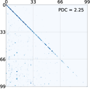
(a) BCE

(b) MiSLAS

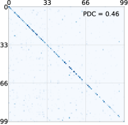
(c) IB

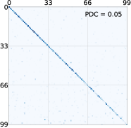
(d) BalCE

Fig. 3: Confusion matrix for each model on CIFAR-100-LT (IF=100). x-axis: predicted label. y-axis: ground truth.

3.1 Datasets

CIFAR100-LT [22] is created from the original CIFAR datasets that have 100 classes with 60K images. The skewness of the dataset is controlled by an Imbalance Factor (IF), which is the ratio between the most and the least frequent classes. We follow previous work[21, 3] to utilize the dataset with $IF=[10,50,100]$ for comprehensive comparisons.

iNaturalist 2018 [23] is the large-scale real-world dataset for LTR with 437.5K images from 8,142 classes. It is extremely imbalanced, with an imbalance factor of 500. We use the official training and validation split in our experiments.

3.2 Implement Details

We use a pre-trained ViT-Base model from MAE and fine-tune it with $32$ (CIFAR-LT) and $128$ (iNat18) resolution. We use AdamW optimizer with momentum $\beta_{1}=0.9$ and $\beta_{2}=0.999$. We train the model for 100 epochs with an effective batch size 1024 and weight decay 0.1. The base learning rate is $1e-3$, which follows cosine decay with 5 warmup epochs. We use Mixup (0.8) and Cutmix (1.0) as augmentation and set the drop path of ViT to 0.1.

3.3 Compared Methods

We adopt the recipe in vanilla ViT[13], DeiT III[14], and MAE[15] to train ViTs. In view of MAE’s excellent performance and low computation consumption, we adopt MAE for our following evaluation. We adopt vanilla CE loss, Binary CE[14], BalCE[9], CB[24], LDAM[21], MiSLAS[11], LADE[17], and IB loss[12] for comprehensive comparisons. We ignore the multi-expert (heavy GPU memory) and contrastive learning (contradictory to MAE) methods.

Table 2 shows the results of different training manners. With the same training image number, the LT is lower than BAL for all recipes. MAE achieves the best on two datasets and learns meaningful features on both datasets (Figure 2). Hence, we select MAE for the following experiments.

Table 3: ViT-B Performance on iNaturalist 2018. Bold indicates the best. $\dagger$: 224 resolution. *:ResNet50 performance.

Method	Many	Med.	Few	Acc	Acc*	PDC
CE	72.45	62.16	56.62	61.03	57.30	0.76
BCE[20]	73.67	65.23	60.41	64.19	59.80	0.66
CB[3]	55.90	62.77	59.07	60.60	61.12	0.42
LDAM[21]	72.61	67.29	63.78	66.45	64.58	0.49
MiSLAS[11]	72.53	64.70	60.45	63.83	71.60	0.64
LADE[10]	64.77	63.49	62.20	63.11	70.00	0.39
IB[12]	54.51	61.91	60.75	60.69	65.39	0.35
BalCE[9]	67.82	68.36	67.34	67.90	69.80	0.27
CE$\dagger$	81.35	72.37	67.45	71.35	-	0.50
BCE[20]$\dagger$	82.54	74.85	70.42	73.89	-	0.42
BalCE[9]$\dagger$	77.83	77.73	76.95	77.43	-	0.18

3.4 LTR Performance with ViT

It is challenging to train ViTs directly on LTR datasets (Table 4), because it is difficult to learn the inductive bias of ViTs and statistical bias of LTR (Eq.2) simultaneously (Table 2). In Table 1, we mainly re-rank different losses of LTR on ViT-Base, which is based on the pre-trained weights on ImageNet. The results in Table 3 are trained from scratch in the MAE manner without pre-trained weights to show the performance gap between ResNet and ViT. We only conduct the architecture comparisons on the iNat18 because ViTs are hard to train from scratch with limited data and resolution, like CIFAR.

As Table 1 & 3 show, BalCE achieves satisfying performance on both datasets, which indicates its effectiveness and generalization. Compared to the performance on ResNet, MiSLAS shows poor Acc and PDC, which means its special design is hard to generalize on ViT. In addition, IB is difficult to train for its numerical instability and thus results in worse performance (7%$\downarrow$). For most proposals, the performance of PDC keeps consistent with Top-1 Acc and Few Acc. However, LDAM has better accuracy and worse PDC compared to CB, which means it alleviates predictive bias slightly. We additionally calculate the variance of PDC for the different unbalanced degrees, as shown in Table 1. From this point of view, BCE obtains the maximum variance with decreasing performance, which suggests its weak adaptability.

Figure 3 presents the visualization with confusion matrix. A larger PDC indicates more centralized off-diagonal elements(e.g., BCE). BalCE makes more balanced predictions with a smaller PDC, which demonstrates PDC is a precise quantitative metric to measure prediction distributions.

Table 4: Performance of ViT-B w/o pretrained weights (CIFAR) or MAE pretraining (iNat18, 128 resolution).

Method	CIFAR100-LT				iNat18
	IF=10		IF=100
	Acc	PDC	Acc	PDC	Acc	PDC
CE	18.69	12.20	11.34	6.74	39.02	1.30
BCE[14]	17.26	13.76	9.86	7.24	42.01	1.25
MiSLAS[11]	18.70	12.40	11.40	9.06	40.23	1.19
BalCE[9]	20.93	1.95	15.89	1.26	42.01	0.43

4 Conclusion

In this paper, we rethink the performance of LTR methods with Vision Transformers and propose a baseline based on unsupervised pre-train to learn imbalanced data. We re-analyze the reasons for LTR methods’ performance variation based on ViT backbone. Furthermore, we propose the PDC to measure the model predictive bias quantitatively, i.e., the predictors prefer to classify images into common classes. Extensive experiments demonstrate the effectiveness of PDC, which provides consistent and more intuitive evaluation.

References

- [1] Olga Russakovsky, Jia Deng, Hao Su, Jonathan Krause, Sanjeev Satheesh, Sean Ma, Zhiheng Huang, Andrej Karpathy, Aditya Khosla, Michael Bernstein, Alexander C. Berg, and Li Fei-Fei, “ImageNet Large Scale Visual Recognition Challenge,” IJCV, vol. 115, no. 3, pp. 211–252, 2015.
- [2] Tsung-Yi Lin, Michael Maire, Serge Belongie, James Hays, Pietro Perona, Deva Ramanan, Piotr Dollár, and C Lawrence Zitnick, “Microsoft coco: Common objects in context,” in ECCV. Springer, 2014, pp. 740–755.
- [3] Yin Cui, Menglin Jia, Tsung-Yi Lin, Yang Song, and Serge Belongie, “Class-balanced loss based on effective number of samples,” in Proceedings of the IEEE/CVF conference on computer vision and pattern recognition, 2019, pp. 9268–9277.
- [4] Ziwei Liu, Zhongqi Miao, Xiaohang Zhan, Jiayun Wang, Boqing Gong, and Stella X Yu, “Large-scale long-tailed recognition in an open world,” in Proceedings of the IEEE/CVF Conference on Computer Vision and Pattern Recognition, 2019, pp. 2537–2546.
- [5] Zhengzhuo Xu, Zenghao Chai, Chun Yuan, et al., “Towards calibrated model for long-tailed visual recognition from prior perspective,” NeurIPS, vol. 34, pp. 7139–7152, 2021.
- [6] Shaoyu Zhang, Chen Chen, Xiujuan Zhang, and Silong Peng, “Label-occurrence-balanced mixup for long-tailed recognition,” in ICASSP 2022-2022 IEEE International Conference on Acoustics, Speech and Signal Processing (ICASSP). IEEE, 2022, pp. 3224–3228.
- [7] Jaehyung Kim, Jongheon Jeong, Jinwoo Shin, et al., “M2m: Imbalanced classification via major-to-minor translation,” in CVPR, 2020, pp. 13896–13905.
- [8] Yongshun Zhang, Xiu-Shen Wei, Boyan Zhou, and Jianxin Wu, “Bag of tricks for long-tailed visual recognition with deep convolutional neural networks,” in AAAI, 2021, pp. 3447–3455.
- [9] Jiawei Ren, Cunjun Yu, Xiao Ma, Haiyu Zhao, Shuai Yi, et al., “Balanced meta-softmax for long-tailed visual recognition,” Advances in neural information processing systems, vol. 33, pp. 4175–4186, 2020.
- [10] Youngkyu Hong, Seungju Han, Kwanghee Choi, Seokjun Seo, Beomsu Kim, and Buru Chang, “Disentangling label distribution for long-tailed visual recognition,” in Proceedings of the IEEE/CVF conference on computer vision and pattern recognition, 2021, pp. 6626–6636.
- [11] Zhisheng Zhong, Jiequan Cui, Shu Liu, and Jiaya Jia, “Improving calibration for long-tailed recognition,” in Proceedings of the IEEE/CVF conference on computer vision and pattern recognition, 2021, pp. 16489–16498.
- [12] Seulki Park, Jongin Lim, Younghan Jeon, and Jin Young Choi, “Influence-balanced loss for imbalanced visual classification,” in Proceedings of the IEEE/CVF International Conference on Computer Vision, 2021, pp. 735–744.
- [13] Alexey Dosovitskiy, Lucas Beyer, Alexander Kolesnikov, Dirk Weissenborn, Xiaohua Zhai, Thomas Unterthiner, Mostafa Dehghani, Matthias Minderer, Georg Heigold, Sylvain Gelly, Jakob Uszkoreit, and Neil Houlsby, “An image is worth 16x16 words: Transformers for image recognition at scale,” in ICLR, 2021.
- [14] Hugo Touvron, Matthieu Cord, and Hervé Jégou, “Deit iii: Revenge of the vit,” in Proceedings of the European Conference on Computer Vision (ECCV), 2022.
- [15] Kaiming He, Xinlei Chen, Saining Xie, Yanghao Li, Piotr Dollár, and Ross Girshick, “Masked autoencoders are scalable vision learners,” in Proceedings of the IEEE/CVF Conference on Computer Vision and Pattern Recognition, 2022, pp. 16000–16009.
- [16] Aditya Krishna Menon, Sadeep Jayasumana, Ankit Singh Rawat, Himanshu Jain, Andreas Veit, and Sanjiv Kumar, “Long-tail learning via logit adjustment,” arXiv preprint arXiv:2007.07314, 2020.
- [17] Youngkyu Hong, Seungju Han, Kwanghee Choi, Seokjun Seo, Beomsu Kim, and Buru Chang, “Disentangling label distribution for long-tailed visual recognition,” in CVPR. 2021, pp. 6626–6636, Computer Vision Foundation / IEEE.
- [18] Renhui Zhang, Tiancheng Lin, Rui Zhang, and Yi Xu, “Solving the long-tailed problem via intra-and inter-category balance,” in ICASSP 2022-2022 IEEE International Conference on Acoustics, Speech and Signal Processing (ICASSP). IEEE, 2022, pp. 2355–2359.
- [19] Jun Li, Zichang Tan, Jun Wan, Zhen Lei, and Guodong Guo, “Nested collaborative learning for long-tailed visual recognition,” in CVPR, 2022, pp. 6949–6958.
- [20] Hugo Touvron, Matthieu Cord, Matthijs Douze, Francisco Massa, Alexandre Sablayrolles, and Hervé Jégou, “Training data-efficient image transformers & distillation through attention,” in International Conference on Machine Learning. PMLR, 2021, pp. 10347–10357.
- [21] Kaidi Cao, Colin Wei, Adrien Gaidon, Nikos Arechiga, and Tengyu Ma, “Learning imbalanced datasets with label-distribution-aware margin loss,” Advances in neural information processing systems, vol. 32, 2019.
- [22] Alex Krizhevsky, Geoffrey Hinton, et al., “Learning multiple layers of features from tiny images,” 2009.
- [23] Grant Van Horn, Oisin Mac Aodha, Yang Song, Yin Cui, Chen Sun, Alex Shepard, Hartwig Adam, Pietro Perona, and Serge Belongie, “The inaturalist species classification and detection dataset,” in Proceedings of the IEEE conference on computer vision and pattern recognition, 2018, pp. 8769–8778.
- [24] Yin Cui, Menglin Jia, Tsung-Yi Lin, Yang Song, and Serge Belongie, “Class-balanced loss based on effective number of samples,” in CVPR, 2019, pp. 9268–9277.