Forecasting Macroeconomic Tail Risk in Real Time:
Do Textual Data Add Value?

We examine the incremental value of news-based data relative to the FRED-MD economic indicators for quantile predictions (now- and forecasts) of employment, output, inflation and consumer sentiment. Our results suggest that news data contain valuable information not captured by economic indicators, particularly for left-tail forecasts. Methods that capture quantile-specific non-linearities produce superior forecasts relative to methods that feature linear predictive relationships. However, adding news-based data substantially increases the performance of quantile-specific linear models, especially in the left tail. Variable importance analyses reveal that left tail predictions are determined by both economic and textual indicators, with the latter having the most pronounced impact on consumer sentiment.

KEYWORDS: Quantile Regression, Textual data, Topic models, Quantile Regression Forests, Gaussian process, Global-local priors

JEL: C53, C55, E27, E37

1 Introduction

Tail risk forecasts of macroeconomic time series provide a more nuanced picture than point forecasts as the former allow for asymmetric links, meaning that the predictive relationship between the target variable and the covariates can vary across quantiles. The focus here is typically on the tails, which are associated with phases of high interest such as economic booms and busts. This is why the literature on macroeconomic forecasting has paid increasing attention to now- and forecasts of quantiles (see, e.g., Manzan, 2015; Korobilis, 2017; Adrian, Boyarchenko, and Giannone, 2019; Carriero, Clark, and Marcellino, 2020; Adams, Adrian, Boyarchenko, and Giannone, 2021; Clark, Huber, Koop, Marcellino, and Pfarrhofer, 2022; Prüser and Huber, 2023).

Another recent development in macroeconomic forecasting is the use of textual data, which provide timely information that may embed complementary signals to (hard) economic indicators (see e.g., Larsen and Thorsrud, 2019; Bybee, Kelly, Manela, and Xiu, 2021; Ellingsen, Larsen, and Thorsrud, 2022). While most studies analyze the benefits of textual predictors for macroeconomic point forecasts, the role of textual predictors for tail forecasting is largely unexplored. In this paper, we study the benefits of such data for forecasting macroeconomic tail risk in real time. In addition, we explore whether the impact of textual predictors differ across forecasting models that feature linear or non-linear predictive relationships.

Our focus is on monthly tail risk (now- and one-step-ahead) forecasts of employment, industrial production, inflation and consumer sentiment between 1999:10 and 2021:12. As data revisions are an important issue in out-of-sample (OOS) macroeconomic forecasting, we use real-time vintages of economic predictors contained in the widely used McCracken and Ng (2016) FRED-MD database. In addition, we use a large set of news attention measures (topic proportions) as predictors, which we obtain from the Correlated Topic Model (CTM). The CTM is an unsupervised machine learning algorithm that estimates our news predictors on almost 800,000 newspaper articles from The New York Times and The Washington Post. The most frequent words within each topic (word cluster) characterize its theme, and the proportion indicates the degree of media coverage of a certain topic at a given point in time. For example, during times of rising energy and consumer prices, a topic about inflation is supposed to gain importance, reflected by a rising topic proportion. The dynamics of topic proportions might further contain signals not captured by traditional economic data. Can such signals be exploited to improve tail risk forecasts? To address this question, we use different sets of predictors: economic predictors only, textual predictors only, and both types of predictors.

Two key insights guided our choice of forecasting models. First, mechanisms to prevent overfitting are necessary for OOS forecasting in high-dimensional settings like ours. We thus use three Bayesian quantile regressions (QR) with different shrinkage priors which assume a linear relationship between the quantile-specific target variables and the covariates. Second, recent studies point to the importance of capturing non-linear predictive relationships. For example, Goulet Coulombe, Leroux, Stevanovic, and Surprenant (2022) consider capturing non-linearities as the “true game changer” of machine learning methods for macroeconomic forecasting, which is corroborated by Medeiros, Vasconcelos, Veiga, and Zilberman (2021) and Clark, Huber, Koop, Marcellino, and Pfarrhofer (2022), finding strong empirical support for tree-based methods. To capture non-linear relationships between the quantile-specific target variables and the covariates, we use non-parametric Bayesian Gaussian Process Regressions (Williams and Rasmussen, 2006) and QR Forests (Meinshausen, 2006). Entertaining both forecasting methods that feature linear and non-linear predictive relationships enables us to evaluate the empirical differences between the model classes.

Our results corroborate empirical evidence that textual data contain valuable incremental information, being particularly useful for predicting events in the left tail of the distribution and less so in its center. This finding is consistent with a narrative that timely news signals are most helpful in extreme economic situations. Our variable importance analyses show that both economic and textual indicators are used for left tail predictions. Importantly, combining text and FRED data can yield sizable gains in forecast accuracy and is never much worse than using FRED data only. Moreover, methods which can capture non-linearities produce better now- and forecasts than those which cannot. However, incorporating textual predictors into models that assume a quantile-specific linear predictive relationship leads to competitive predictions, especially for the left tail. We finally observe substantial forecast accuracy gains for consumer sentiment when using textual data, which is consistent with the notion that news data are important in forming household expectations (Larsen, Thorsrud, and Zhulanova, 2021).

The paper proceeds as follows. Section 2 lays out our methodology. Section 3 outlines our forecasting setup, introduces our predictors, and presents our forecast results. Section 4 concludes. Additional material is relegated in the appendix.

2 Methodology

2.1 Forecasting methods

2.1.1 Bayesian Quantile Regression

In settings with many regressors, Bayesian shrinkage alleviates overfitting and thus noisy forecasts. Recently, Carriero, Clark, and Marcellino (2022) showed the importance of using shrinkage for QR in empirical macroeconomics. For Bayesian estimation, we use the mixture representation established by Yu and Moyeed (2001). For a given variable $y$ of interest that is to be predicted for quantile $\tau$ at horizon $h$, the Bayesian QR can be stated as

$$y_{t+h}=\mathbf{x}_{t}\mathbf{\beta}_{\tau}+\varepsilon_{\tau,t+h}\text{,}$$ (1)

where $\left\{x_{t}\right\}_{t=1}^{T-h}$ is a $K$-dimensional vector of predictors, and $K$ denotes the set of predictors that depends on the setting (FRED predictors only, textual predictors only, or FRED and textual predictors together). Let $\beta_{\tau}$ denote a $K$-dimensional vector of quantile-specific regression coefficients, and $\varepsilon_{\tau,t+h}$ has a mixture representation. The shocks are assumed to follow an asymmetric Laplace distribution (Yu and Moyeed, 2001).

Using the mixture representation, we can rewrite the QR model (1) as

$$y_{t+h}=\mathbf{x}_{t}\mathbf{\beta}_{\tau}+\theta_{\tau}z_{\tau,t+h}+\kappa_{\tau}\sqrt{\sigma_{\tau,h}z_{\tau,t+h}}u_{t+h\text{,}}$$ (2)

where $z_{\tau,t+h}$ is exponentially distributed with scale parameter $\sigma_{\tau,h};$ $\theta_{\tau}$ and $\kappa_{\tau}$ are quantile-specific fixed parameters, $u_{t+h}$ is i.i.d. standard normal.

Posterior inference requires specifying a likelihood and eliciting priors for the coefficients. As Markov Chain Monte Carlo estimation is slow in high dimensions, we use fast variational Bayes approximations for posterior inference. In the interest of brevity we do not give full details of the estimation, but note that, by introducing auxiliary latent variables, the likelihood is conditionally Gaussian and the errors are conditionally heteroskedastic. The shrinkage priors we consider fall into the class of global-local shrinkage priors, where the prior variance comprises one global term pertaining to all coefficients and another coefficient-specific term. The three shrinkage priors we use can be written in the general form

$$\mathbf{\beta}_{\tau}|\psi_{\tau_{1}},\ldots,\psi_{\tau_{K}},\lambda_{\tau}\sim\prod\limits_{j=1}^{K}\mathcal{N}\left(0,\psi_{\tau j}\lambda_{\tau}\right),\text{ }\psi_{\tau j}\sim u,\text{ \ }\lambda_{\tau}\sim\pi\text{,}$$ (3)

where $\lambda_{\tau}$ denotes a quantile-specific global shrinkage parameter and $\psi_{\tau j}$ are quantile-specific local scaling parameters that control the coefficient-specific shrinkage intensities. Different shrinkage priors are generated by choosing different mixing densities via the functions $u$ and $\pi$. We consider the three following shrinkage priors that are popular choices in macroeconomic forecasting; see, e.g., Huber and Feldkircher (2019), Cross, Hou, and Poon (2020), and Prüser (2023):

• Ridge: The Ridge prior collapses to a purely global shrinkage prior since all local scaling parameters are set equal to $1$. The global shrinkage parameter follows an inverse Gamma distribution. Formally, we thus have: $\psi_{\tau j}=1$    $\forall\tau,j$ and $\lambda_{\tau}\sim\mathcal{IG}\left(e_{0},e_{1}\right)$. We choose the hyperparameters $e_{0}=e_{1}=0$, thus shrinking all coefficients towards zero in the same vein. Overall, the Ridge prior offers a comparatively low degree of flexibility for variable-specific deviations from the global shrinkage pattern. This prior is supposed to work well when many predictors are relevant, being consistent with a dense representation of the prediction problem.

• Horseshoe: In contrast to the Ridge prior, the Horseshoe prior (Carvalho, Polson, and Scott, 2010) offers variable-specific shrinkage. The Horseshoe sets $u$ and $\pi$ to half-Cauchy distributions, respectively: $\sqrt{\psi_{\tau j}}\sim\mathcal{C}^{+}\left(0,1\right)$ and $\sqrt{\lambda_{\tau}}\sim\mathcal{C}^{+}\left(0,1\right)$. An advantage of the Horseshoe prior is that it does not require the researcher to elicit any tuning parameters. The Horseshoe prior has been shown to have excellent posterior contraction properties, see, e.g., Ghosh, Tang, Ghosh, and Chakrabarti (2016). The Horseshoe prior spikes at zero and has fat tails. Hence, it is supposed to shrink small coefficients of unimportant predictors to zero, but (in relative terms) large coefficients of the informative predictors are not shrunk much. Accordingly, the Horseshoe prior should work well when only a small number out of the pool of predictors is useful, consistent with a sparse representation of the prediction problem. Kohns and Szendrei (2021) found the Horseshoe prior to work well for quantile forecasting with many predictors.

• Lasso: The Lasso prior is a special case of the Normal-Gamma prior of Brown and Griffin (2010). The Lasso involves setting $u$ and $\pi$ to Gamma distributions: $\psi_{\tau j}\sim\mathcal{G}\left(1,\lambda_{\tau}/2\right)$ and $\lambda_{\tau}\sim\mathcal{G}\left(c_{0},d_{0}\right)$. We set the hyperparameters $c_{0}=d_{0}=0$, implying heavy global shrinkage. The marginal prior of the coefficients exhibits fat tails. Overall, the Lasso prior offers richer shrinkage patterns than Horseshoe and Ridge.

2.1.2 Gaussian Process Regressions

The Gaussian Process Regression (Williams and Rasmussen, 2006) is a non-parametric method that was recently used for inflation forecasting by Clark, Huber, Koop, and Marcellino (2022). It elicits a process prior on the function $g_{\tau}\left(\mathbf{x}_{t}\right):$

$$g_{\tau}\left(\mathbf{x}_{t}\right)\sim\mathcal{GP}\left(\mu_{\tau}\left(\mathbf{x}_{t}\right),\mathcal{K}\left(\mathbf{x}_{t},\mathbf{x}_{\mathfrak{t}}\right)\right)\text{,}$$ (4)

where we set the mean function $\mu_{\tau}\left(\mathbf{x}_{t}\right)$ to zero. The kernel function $\mathcal{K}\left(\mathbf{x}_{t},\mathbf{x}_{\mathfrak{t}}^{{}^{\prime}}\right)$ describes the relationship between $\mathbf{x}_{t}$ and $\mathbf{x}_{\mathfrak{t}}$, for $t$, $\mathfrak{t=}1,\ldots,T$.

As $\mathbf{x}_{t}$ is observed at discrete points in time, $\mathbf{g}_{\tau}=\left(g_{\tau}\left(\mathbf{x}_{1}\right),\ldots,g_{\tau}\left(\mathbf{x}_{T}\right)\right)^{\prime}$:

$$\mathbf{g}_{\tau}\sim\mathcal{N}\left(\mathbf{0}_{T},\mathbf{K}\left(\mathbf{w}\right)\right)\text{, }$$ (5)

where $\mathbf{K}\left(\mathbf{w}\right)$ refers to a $T\times T$-dimensional matrix with $\left(t,\mathfrak{t}\right)$-th element $\mathcal{K}\left(\mathbf{x}_{t},\mathbf{x}_{\mathfrak{t}}\right)$.

The type of kernel determines the estimated function. We choose a squared exponential kernel:

$$\mathcal{K}\left(\mathbf{x}_{t},\mathbf{x}_{\mathfrak{t}}\right)=w_{1}\times e^{-\frac{w_{2}}{2}\left\|\mathbf{x}_{t}-\mathbf{x}_{\mathfrak{t}}\right\|^{2}}\text{,}$$ (6)

where we follow Chaudhuri, Kakde, Sadek, Gonzalez, and Kong (2017) for setting the hyperparameters $\mathbf{w=}\left(w_{1},w_{2}\right)^{{}^{\prime}}$, which govern the smoothness of the function.

Above we have outlined the function-space view of the GP regression. In the alternative weight-space view, which is convenient for estimation, the GP regression can be expressed as

$$\mathbf{y}=\mathbf{Z\gamma}_{\tau}+\mathbf{\varepsilon}\text{,}$$ (7)

where $\mathbf{y}$ denotes the stacked dependent variables, $\mathbf{Z}$ represents the lower Cholesky factor of $\mathbf{K}$, and $\mathbf{\gamma}_{\tau}\sim\mathcal{N}\left(\mathbf{0}_{T},\mathbf{I}_{T}\right)$.

2.1.3 Quantile Regression Forests

Our last forecasting method is a frequentist non-parametric method, namely QR Forests, an extension of Random Forests (Breiman, 2001) for conditional point estimation to conditional quantile estimation based on an ensemble of trees (Meinshausen, 2006). Random Forests and QR Forests capture non-linear predictive relationships and, especially due to this feature, have been found to perform well in macroeconomic forecasting (see, e.g., Medeiros, Vasconcelos, Veiga, and Zilberman, 2021; Clark, Huber, Koop, Marcellino, and Pfarrhofer, 2022).

Random Forests grow a large number of trees by using $n$ independent observations

$$\left(Y_{i},X_{i}\right),i=1,\ldots,n\text{,}$$

where $Y$ is the variable of interest and $X$ is a (possibly high-dimensional) predictor variable. For ease of notation we drop time subscripts. For each tree and in each node, Random Forests use a random subset of predictors to split on. The intuition of this random selection is to de-correlate the trees and thus to decrease the variance of the forecasts. In Random Forests, the conditional mean prediction of $Y$, given $X=x$, is generated as the weighted sum over all observations:

$$\widehat{\mu}\left(x\right)=\sum\limits_{i=1}^{n}w_{i}\left(x\right)Y_{i}\text{,}$$ (8)

where the weights $w_{i}\left(x\right)$ are computed over the collection of trees. In each tree, the conditional mean prediction is the simple average of all observations that fall into the same leaf when dropping down $x$; the remaining observations are neglected.

Meinshausen (2006) extended the Random Forests to QR Forests. The conditional distribution function $y$, given $X=x$, is

$$F\left(y|X=x\right)=P\left(Y\leq y|X=x\right)=\mathbbm{E}\left(\mathbbm{1}_{\left\{Y\leq y\right\}}|X=x\right)\text{.}$$ (9)

Instead of approximating the conditional mean $\mathbbm{E}\left(Y|X=x\right)$ in case of Random Forests, for QR Forests, $\mathbbm{E}\left(\mathbbm{1}_{\left\{Y\leq y\right\}}|X=x\right)$ is approximated by the weighted mean over the observations $\mathbbm{1}_{\left\{Y\leq y\right\}}$,

$$\widehat{F}\left(y|X=x\right)=\sum\limits_{i=1}^{n}w_{i}\left(x\right)\mathbbm{1}_{\left\{Y\leq y\right\}}\text{,}$$ (10)

where $w_{i}\left(x\right)$ are the same weights as for Random Forests. Based on $\widehat{F}\left(y|X=x\right)$, we can estimate the desired conditional $\alpha$-quantile $Q_{\alpha}\left(x\right)$ as

$$\widehat{Q}_{\alpha}\left(x\right)=\inf\left(y:\widehat{F}\left(y|X=x\right)\geq\alpha\right)\text{.}$$ (11)

An important difference between QR Forests and Random Forests is that, for each node in each tree, Random Forests keep just the mean of the observations that fall into the respective node, while QR Forests store the values of all observations in the respective node for computing the conditional distribution.

2.2 Probabilistic topic models

We use topic models to extract information from newspaper articles and to create textual predictors. These models are predominantly data-driven and use a probabilistic approach to identify themes within a large set of written documents. In contrast to dictionary-based and/or Boolean approaches, topic models are initially context-agnostic, finding word clusters (topics) solely based on the co-occurrence of words.

The most prominent topic model is latent Dirichlet allocation (LDA) by Blei, Ng, and Jordan (2003). It posits that documents are generated by a stochastic process where each text is a mixture of latent topics and each topic is a probability distribution over the same vocabulary, but with different probabilities for each word. Despite its prominence and advantages, LDA cannot account for the fact that certain topics tend to co-occur together within documents (e.g., inflation and commodity prices). We therefore use the more sophisticated correlated topic model (CTM) by Blei and Lafferty (2007) which has been developed to address this limitation.

Figure 1 shows a graphical model of the generative process assumed by the CTM where edges denote dependency, nodes are random variables, and plates are replicated variables. The only observable variables of the model are the words ($w$).

Figure 1: Generative process of the CTM based on Blei and Lafferty (2007).

The key difference between LDA and the CTM is the assumption for the topic proportions, $\theta_{d}$. The CTM assumes that topic proportions arise from a logistic normal distribution—which has a mean vector ($\mu$) and a covariance matrix ($\Sigma$)—in contrast to LDA, which assumes that topic proportions arise from a Dirichlet distribution. Consistent with the more realistic assumptions of correlating topics, the CTM yields higher values for statistics that measure the predictive performance regarding unseen documents (Blei and Lafferty, 2007). The generative process of the CTM can be written as follows (local mathematical notation):

1. K topics of length V (unique vocabulary) are drawn from the Dirichlet distribution with input vector $\gamma$:

   $$\beta_{k}\sim Dir(\gamma).$$

2. For each document d, topic proportions ($\theta_{d}$) of length K are drawn from the logistic normal distribution:

   $$\eta_{d} \sim\mathcal{N}(\mu,\Sigma)$$

   $$\theta_{d,k} =\frac{\exp{(\eta_{d,k})}}{\sum_{i=1}^{k}\exp{(\eta_{d,i})}}.$$

   1. For each word $n$, a topic assignment is drawn from the multinomial distribution:

      $$z_{d,n}|\theta_{d}\sim Mult(\theta_{d}).$$

   2. Each word is drawn from the multinomial distribution:

      $$w_{d,n}|z_{d,n},\beta_{1:K}\sim Mult(\beta_{z_{d,n}}).$$

We use the partially collapsed variational EM algorithm by Roberts, Stewart, and Airoldi (2016) to estimate the CTM. The approach is implemented in the R-package stm by Roberts, Stewart, and Tingley (2019). We are particularly interested in estimating $\theta_{d}$, namely the topic proportions of each document, whose aggregates serve as our textual predictors; see Section 3.2.2.

3 Empirical work

3.1 Forecasting setup

We generate monthly quantile now- and one-month-ahead forecasts for employment, inflation, industrial production, and consumer sentiment. Depending on the setting, we incorporate FRED predictors, textual predictors, or both together. We detail our predictors in Section 3.2. In addition, all model specifications include 12 lags of the respective (transformed) variable of interest.

For our variables of interest and the FRED predictors we use vintage data from the database of McCracken and Ng (2016). Our estimation sample starts in 1980:06, when the news data series start. We run recursive estimations based on an expanding window. Our evaluation periods ranges from 1999:10 to 2021:12.

For nowcasts of a given month, we include macroeconomic predictors from the month before due to the publication lag, while we include textual and financial predictors from the month to be forecasted. For example, if we are at the end of December and produce a nowcast for December, we use the macroeconomic predictors from November released in December, and the financial and textual predictors from December. Similarly, for one-month-ahead forecasts, if we are at the end of December and produce a prediction for January, we use the macroeconomic predictors from November released in December and the financial and textual predictors from December.

We evaluate our forecasting models with the quantile score (QS), which is computed as

$$QS_{\tau,t+h}=\left(y_{t+h}-Q_{\tau,t+h}\right)\left(\tau-\mathbbm{1}_{\left\{y_{t+h}\leq Q_{\tau,t+h}\right\}}\right)\text{,}$$ (12)

where $y_{t+h}$ is the actual outcome of the variable of interest in $t+h$, $Q_{\tau,t+h}$ denotes the forecast of quantile $\tau$ for $t+h$. The indicator function $\mathbbm{1}_{\left\{y_{t+h}\leq Q_{\tau,t+h}\right\}}$ takes on a value of $1$ if the outcome is not higher than the quantile forecast, and $0$ otherwise.

3.2 Predictor sets

3.2.1 Economic predictors

Our macroeconomic predictors are from the McCracken and Ng (2016) FRED-MD database. We pick all predictors from the database that are available at the end of the sample as well as the beginning. The predictors can be classified into eight categories: (i) output and income, (ii) labor market, (iii) housing, (iv) consumption, orders, and inventories, (v) money and credit, (vi) interest and exchange rates, (vii) prices, and (viii) stock market. For the classification of the variables, see https://www.ssc.wisc.edu/~bhansen/econometrics/FRED-MD_description.pdf.

3.2.2 Textual predictors

We used the legal database LexisNexis to download 793,013 economically related newspaper articles from The New York Times and The Washington Post between 1980:06 and 2021:12. We then conducted Part-of-Speech-Tagging (Benoit and Matsuo, 2022) to remove anything but nouns from the articles. Our reason for this choice is that topic models aim to summarize the content of documents, which is predominantly described by nouns, in contrast to sentiment analysis which aims to describe the documents’ tone. In addition, Martin and Johnson (2015) found highest values of semantic coherence when using a nouns-only approach, a metric that strongly correlates with human judgement.

We tokenized the documents into single words, removed punctuation, numbers, symbols, stopwords, etc., and constructed a document-term matrix (dtm). A dtm counts how often a certain word (column) occurs within a certain document (row). We then computed term-frequency inverse-document-frequency values for each word to extract the 10,000 most relevant terms until 1999:09. The final dtm served as the input for the CTM. In addition, the number of topics $K$ has to be given as an input by the researcher. Following Larsen and Thorsrud (2019), Thorsrud (2020) and Ellingsen, Larsen, and Thorsrud (2022), we set the number of topics to 80.

We estimated for each document on each day 80 topic proportions ($\hat{\theta}_{d}$) based on the newspaper articles until 1999:09. After then, we computed the topic proportions OOS to exclude any look-ahead bias, similar to Ellingsen, Larsen, and Thorsrud (2022). Finally, for a given month, we computed the simple average over all documents’ estimated topic proportions. We use the averages of topic proportions as news attention measures in our empirical analyses. Figure 2 shows the trajectories of four selected topics.. The figures show that our topics capture important political and economic events such as several debt crises in Mexico, Asia and Europe (Topic 9), the beginning of the Gulf War in 1991 (Topic 27) and the Great Recession which emanated in the housing market (Topic 46).

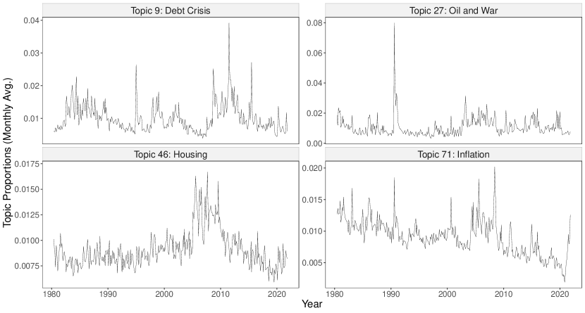
Figure 2: Four selected topic proportions (monthly averages) based on the CTM.

Our forecast results remain robust for different choices. For instance, following Adämmer and Schüssler (2020), who use the CTM and a similar corpus, we computed 100 instead of 80 topics. In addition, the CTM is nested within the more sophisticated structural topic model (STM) by Roberts, Stewart, and Airoldi (2016), which further allows to include covariates. We estimated an STM to account for our two different news sources. Finally, we estimated all models with 15,000 unique words.

3.3 Forecast results

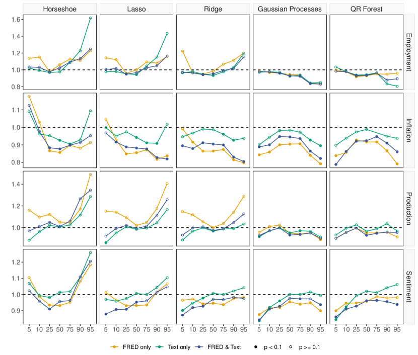
Figure 3: Nowcast (h = 0) quantile scores. The dotted black horizontal line shows the quantile score of the AR(1) benchmark which is standardized to 1.0. Scores below (above) 1.0 indicate more (less) precise forecasts for a given quantile compared to the AR(1) benchmark. Inside colored dots indicate significantly higher forecast accuracy compared to the AR(1) benchmark according to a one-tailed Diebold and Mariano (1995) test at the $10\%$ level.

Figure 3 and 4 summarize the results for the now- and the one-month-ahead forecasts, respectively. Forecast accuracy is assessed by quantile scores across different quantiles $\tau$: $\tau$ = 5%, 10%, 25%, 50%, 75%, 90%, 95%. A quantile AR(1) model serves as our benchmark. Quantile scores below (above) one indicate more (less) precise forecasts compared to the benchmark model.

We observe the following patterns: first, concerning the news attention measures, the combination of macroeconomic predictors and textual predictors leads to accuracy gains in many cases compared to the setting with macroeconomic or textual predictors only. In the cases where adding textual predictors does not improve forecast performance, it does not materially harm either. The incremental value from adding textual predictors is pronounced in the tails and more so for the forecasting models that feature a linear predictive relationship. Improved tail forecasting with textual data points to a scenario where textual predictors are especially helpful in extreme economic environments, where timely news data might reflect the economic overall picture and are useful predictors for macroeconomic variables. In times like the Great Recession or the COVID-19 pandemic, developments like uncertainty and political changes might have been more closely captured than by hard economic indicators. In Horseshoe, Lasso and Ridge, textual predictors might compensate the non-modeled complexity in form of a non-linear predictive relationship.

Second, in both figures, the quantile scores of the linear models tend to be U-shaped, whereas the quantile scores of the models that feature a non-linear predictive relationships are mainly hump-shaped. Hence, the linear models generate comparatively precise forecasts in the center of the distribution whereas the non-linear models shine especially in forecasting the tails. In either case, the addition of textual data has a lower impact in the center of the distribution than in the tails.

Third, within the class of methods that feature a non-linear predictive relationship, Gaussian processes have a slight edge over QR forests across variables and quantiles, with more cases where they produce more precise and significantly better forecasts than an AR(1) model according to the Diebold and Mariano (1995) test. Within the class of linear models, the Horseshoe shrinkage prior overall underperforms the Lasso and Ridge shrinkage priors in the tails. Ridge, as a purely global shrinkage prior, is at least on par with Lasso which, as a global-local shrinkage prior, applies predictor-specific shrinkage. Hence, the richer shrinkage patterns offered by Lasso do not pay off in this analysis. These results are consistent with a dense representation of the prediction problem where many weak predictors are relevant rather than with a sparse structure where few important predictors can be selected and the others are dismissed (Giannone, Lenza, and Primiceri, 2021).

Fourth, we find the following key patterns of predictability for our four target variables. For employment, we observe substantial outperformance in the right tail for now- and forecasts in case of the Gaussian processes; regarding inflation now- and forecasts, accuracy gains are most pronounced in the tails for Gaussian processes and QR forests. Here, Ridge becomes competitive with these methods once textual predictors are added. For industrial production now- and forecasts, overall Gaussian processes exhibit the strongest forecast performance, with QR forests as a close second. Again, the methods with a linear predictive relationship become competitive once textual predictors are added. For consumer sentiment (now- and forecasts), quantile scores markedly improve in the left tail when textual predictors are added, in particular for the methods with a linear predictive relationship. This result is interesting from an information processing aspect, supporting the notion that news data play an important role for households in forming their expectations (Larsen, Thorsrud, and Zhulanova, 2021).

3.4 Which predictors determine the quantile forecasts?

Since we include forecasting methods that feature non-linear predictive relationships, it is not obvious how to pin down the marginal effect of any predictor on the variable of interest. Further, we use heterogeneous forecasting methods, and we wish to ensure comparability for measures of predictor importance across the methods. To accomplish this task and to shed light on the predictors with the highest impact, for each forecasting model, we rely on a linear approximation to the predictive distribution as proposed by Woody, Carvalho, and Murray (2021). Concretely, we aim to approximate the quantile predictions $Q_{\tau,t+h}$ with a linear regression model that uses regularization. For each quantile $\tau$, the following Lasso-type optimization problem is solved:

$$\mathbf{\beta}_{\tau}^{\ast}=\underset{\mathbf{\beta}_{\tau}}{\arg\min}\sum\limits_{t=t_{0}}^{T-h}\left(Q_{\tau,t+h}-\mathbf{\beta}_{\tau}^{\prime}\mathbf{x}_{t}\right)^{2}+\lambda\sum\limits_{j=1}^{K}\left|\beta_{\tau,j}\right|\text{,}$$ (13)

where $t_{0}$ denotes the beginning of the hold-out period, $\mathbf{\beta}_{\tau}=\left(\beta_{\tau,1},\ldots,\beta_{\tau,K}\right)^{\prime}$ denotes the vector of coefficients, and $\lambda\geq 0$ is a penalty parameter that controls the shrinkage intensity and is chosen via cross-validation. For the predictor importance analysis we use our most comprehensive set of predictor variables, including both FRED and textual predictors. We focus on the $10\%$-quantile because our previous analysis has shown the most interesting patterns in the lower tails. Figure 5 and Figure 6 report the five most influential predictors at the $10\%$-quantile for now- and forecasts, respectively. Importance is measured by the absolute values of the coefficients associated with the (standardized) predictors. Overall, we observe a fair degree of overlap across the forecasting methods regarding the most influential variables.

For employment, mostly FRED predictors related to the labor market are included in the top five. Further, both Ridge and the Gaussian Process Regressions include the “Regulation and Law” news topic among the most important predictors; for inflation, FRED predictors related to prices are in the lead. Regarding news predictors, Gaussian processes and QR Forests agree on the “Housing” topic for one-month-ahead forecasts; for production, the most influential FRED predictors are spread among variables related to the labor market, money & credit, and housing. For nowcasts of production, Horseshoe and Lasso select the “State of the Economy” topic as an important predictor. For one-month-ahead forecasts of production, in Lasso, Ridge, and Gaussian processes, the “Regulation and Law” topic appears in the top five; for consumer sentiment, FRED variables related to interest and exchange rates prevail. For nowcasts, all forecasting methods select the “State of Economy” topic as top five predictor. For one-month-ahead forecasts of consumer sentiment, all forecasting methods except Lasso agree on the “Debt Crisis” topic. Especially for consumer sentiment forecasts, the relatively high number of news predictors in the top five is apparent and consistent with the strong forecast performance of textual predictors for sentiment (see Figure 4). Altogether, the predictors that appear as most influential for the respective target variable make sense from an economic perspective.

Another interesting piece of information is how many FRED and textual predictors were chosen in the Lasso-regression (13). Figure 7 and 8 show the number of nonzero coefficients for the now- and one-step-ahead forecasts, respectively. We focus on the 10%, 50% and 90% quantiles here. Overall, the structure for the one-step-ahead forecasts is substantially sparser than in case of the nowcasts. Across different target variables and quantiles, the structure of included FRED and textual predictors is balanced. However, we observe a comparatively high portion of selected textual predictors for consumer sentiment, corroborating their important role for this variable.

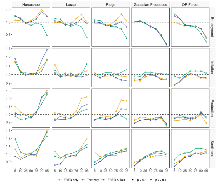
Figure 4: One-step-ahead (h = 1) quantile scores. The dotted black horizontal line shows the quantile score of the AR(1) benchmark which is standardized to 1.0. Scores below (above) 1.0 indicate more (less) precise forecasts for a given quantile compared to the AR(1) benchmark. Inside colored dots indicate significantly higher forecast accuracy compared to the AR(1) benchmark according to a one-tailed Diebold and Mariano (1995) test at the $10\%$ level.

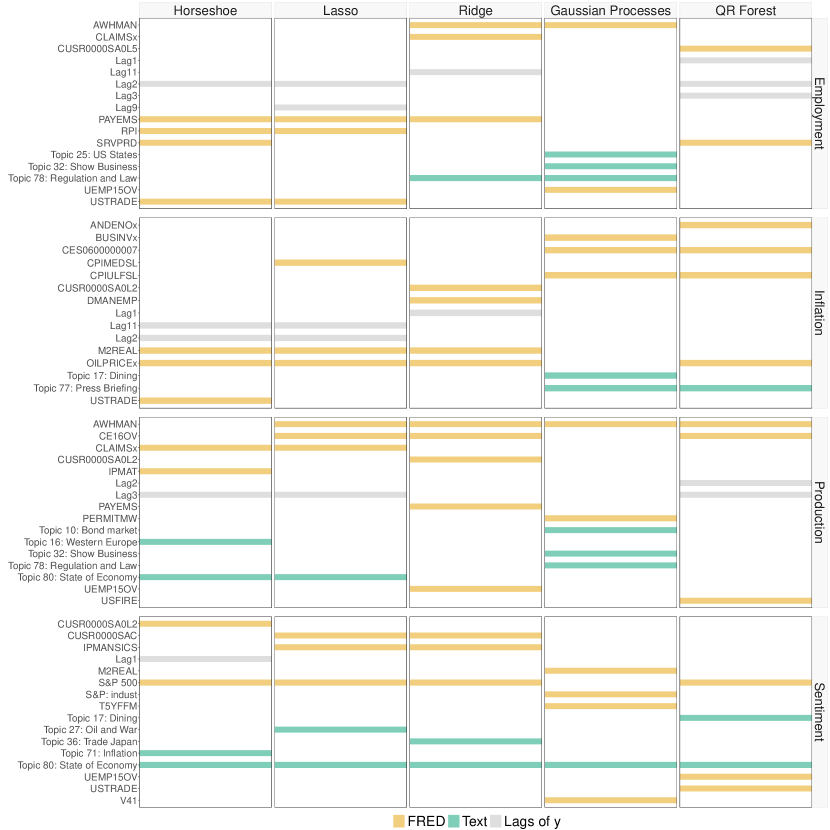
Figure 5: Variable importance for nowcasts at the $10\%$-quantile $(h=0$, $\tau=10\%)$.

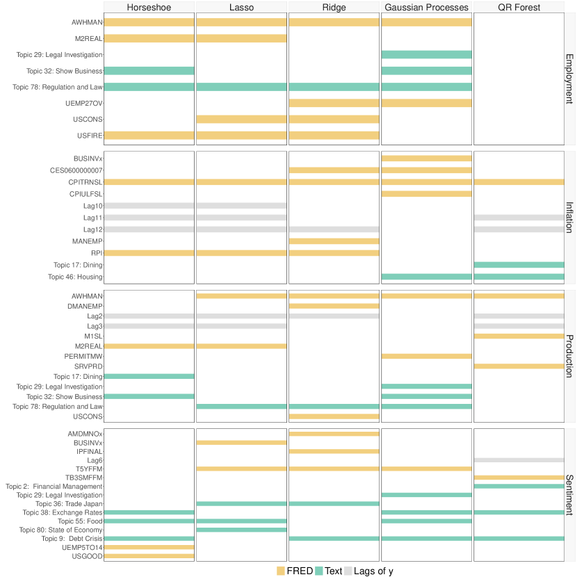
Figure 6: Variable importance for one-step-ahead forecasts at the $10\%$-quantile $(h=1,\tau=10\%)$.

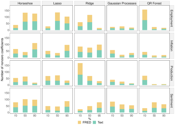
Figure 7: Variable selection for nowcasts $(h=0)$ based on Equation (13).

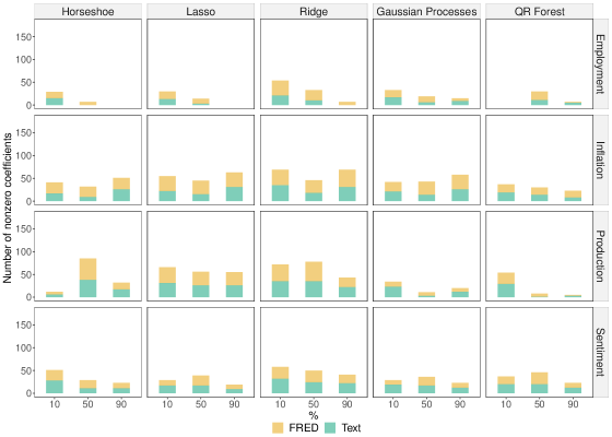
Figure 8: Variable selection for one-step-ahead forecasts $(h=1)$ based on Equation (13).

4 Concluding remarks

We have analyzed the value added by textual predictors for quantile now- and forecasts of macroeconomic time series. Our high-dimensional setup comprised forecasting methods with both linear and non-linear quantile-specific predictive relationships, and we considered different sets of predictors.

Overall, Gaussian Process Regressions and QR Forests prevailed in terms of tail forecast accuracy, suggesting that non-linear predictive relationships are a promising route to follow in tail forecasting. Although forecast performance varied across quantiles and target variables, altogether, combinations of FRED and textual predictors produced the most accurate forecasts, especially in the tails. In cases where adding the news attention measures did not provide gains in forecast accuracy, they were not detrimental either. Hence, the benefits from incorporating textual data tend to outweigh the risks.

Appendix A Topics and their keywords

Topic 1 Topic 2 Topic 3 Topic 4 Topic 5 Topic 6 Topic 7 Topic 8 Topic 9 Topic 10 bill target committee dollar sale worker date country debt bond legislation balance chairman currency unit union start world mexico percent measure release issue exchange auto labor correction nation brazil rate amendment goal vote yen maker wage schedule government crisis yield provision ratio senator mark analyst strike delay economy payment note Topic 11 Topic 12 Topic 13 Topic 14 Topic 15 Topic 16 Topic 17 Topic 18 Topic 19 Topic 20 president member subc israel percent germany restaurant car rate america office board appropriation peace increase france wine truck loan problem director plan subcommittee lebanon figure britain bar vehicle interest question staff commission budget egypt decline west dinner bus mortgage idea washington proposal committee syria rate east coffee driver credit fact Topic 21 Topic 22 Topic 23 Topic 24 Topic 25 Topic 26 Topic 27 Topic 28 Topic 29 Topic 30 police weapon book speech state south oil cent lawyer quarter violence arm newspaper event california black iraq contract case share death missile paper crowd jersey africa iran gasoline charge percent attack korea magazine visit governor minority barrel future official profit security defense page message texas white gas delivery investigation loss Topic 31 Topic 32 Topic 33 Topic 34 Topic 35 Topic 36 Topic 37 Topic 38 Topic 39 Topic 40 government show tax stock child trade benefit gold group hotel poland los budget share family japan employee dollar organization room protest angeles cut point life export cost york community tourist demonstration san taxis index parent import worker rate church visitor leader film spending investor mother product pay trading movement beach Topic 41 Topic 42 Topic 43 Topic 44 Topic 45 Topic 46 Topic 47 Topic 48 Topic 49 Topic 50 building computer campaign drug official home job city bank report housing technology candidate crime policy house work york loan study project system voter police administration property force resident banking number construction machine election prison issue estate unemployment neighborhood institution research apartment information poll officer effort owner employment mayor saving survey Topic 51 Topic 52 Topic 53 Topic 54 Topic 55 Topic 56 Topic 57 Topic 58 Topic 59 Topic 60 agreement plane china united food party program health rate market talk space beijing states meat election government care economy future negotiation ship taiwan washington fruit leader agency insurance growth firm deal aircraft hong cuba animal government welfare hospital inflation investor side air kong country product power money doctor economist broker Topic 61 Topic 62 Topic 63 Topic 64 Topic 65 Topic 66 Topic 67 Topic 68 Topic 69 Topic 70 school company service woman aid store plant fund county business student firm airline man guerrilla chain steel money area industry education executive card life nicaragua retailer power investment maryland economy college deal fare friend rebel customer energy investor official corporation teacher management phone guy government shopping utility return washington executive Topic 71 Topic 72 Topic 73 Topic 74 Topic 75 Topic 76 Topic 77 Topic 78 Topic 79 Topic 80 price union vietnam farm building water meeting law war nation consumer soviet refugee farmer room land conference court force effort cost russia immigrant crop wall mile news case troop part increase moscow kong grain floor town leader rule army million producer republic hong land street area statement regulation military end

Appendix B Variable transformations

ID	FRED Code	Description	Transformation Codes	Financial
1	RPI	Real Personal Income	5
2	W875RX1	Real personal income ex transfer receipts	5
4	CMRMTSPLx	Real Manu. and Trade Industries Sales	5
5	RETAILx	Retail and Food Services Sales	5
6	INDPRO	IP Index	5
7	IPFPNSS	IP: Final Products and Nonindustrial Supplies	5
8	IPFINAL	IP: Final Products (Market Group)	5
9	IPCONGD	IP: Consumer Goods	5
13	IPMAT	IP: Materials	5
16	IPMANSICS	IP: Manufacturing (SIC)	5
20	CUMFNS	Capacity Utilization: Manufacturing	2
23	CLF16OV	Civilian Labor Force	5
24	CE16OV	Civilian Employment	5
25	UNRATE	Civilian Unemployment Rate	2
26	UEMPMEAN	Average Duration of Unemployment (Weeks)	2
27	UEMPLT5	Civilians Unemployed - Less Than 5 Weeks	5
28	UEMP5TO14	Civilians Unemployed for 5-14 Weeks	5
29	UEMP15OV	Civilians Unemployed - 15 Weeks & Over	5
30	UEMP15T26	Civilians Unemployed for 15-26 Weeks	5
31	UEMP27OV	Civilians Unemployed for 27 Weeks and Over	5
32	CLAIMSx	Initial Claims	5
33	PAYEMS	All Employees: Total nonfarm	5
34	USGOOD	All Employees: Goods-Producing Industries	5
35	CES1021000001	All Employees: Mining and Logging: Mining	5
36	USCONS	All Employees: Construction	5
37	MANEMP	All Employees: Manufacturing	5
38	DMANEMP	All Employees: Durable goods	5
39	NDMANEMP	All Employees: Nondurable goods	5
40	SRVPRD	All Employees: Service-Providing Industries	5
42	USWTRADE	All Employees: Wholesale Trade	5
43	USTRADE	All Employees: Retail Trade	5
44	USFIRE	All Employees: Financial Activities	5
45	USGOVT	All Employees: Government	5
46	CES0600000007	Avg Weekly Hours : Goods-Producing	1
47	AWOTMAN	Avg Weekly Overtime Hours : Manufacturing	2
48	AWHMAN	Avg Weekly Hours : Manufacturing	1
50	HOUST	Housing Starts: Total New Privately Owned	4
51	HOUSTNE	Housing Starts, Northeast	4
52	HOUSTMW	Housing Starts, Midwest	4
53	HOUSTS	Housing Starts, South	4
54	HOUSTW	Housing Starts, West	4
55	PERMIT	New Private Housing Permits (SAAR)	4
56	PERMITNE	New Private Housing Permits, Northeast (SAAR)	4
57	PERMITMW	New Private Housing Permits, Midwest (SAAR)	4
58	PERMITS	New Private Housing Permits, South (SAAR)	4
59	PERMITW	New Private Housing Permits, West (SAAR)	4
65	AMDMNOx	New Orders for Durable Goods	5
66	ANDENOx	New Orders for Nondefense Capital Goods	5
67	AMDMUOx	Un lled Orders for Durable Goods	5
68	BUSINVx	Total Business Inventories	5
69	ISRATIOx	Total Business: Inventories to Sales Ratio	2
70	M1SL	M1 Money Stock	6

ID	FRED Code	Description	Transformation Codes	Financial
71	M2SL	M2 Money Stock	6
72	M2REAL	Real M2 Money Stock	5
74	TOTRESNS	Total Reserves of Depository Institutions	6
75	NONBORRES	Reserves Of Depository Institutions	7
76	BUSLOANS	Commercial and Industrial Loans	6
77	REALLN	Real Estate Loans at All Commercial Banks	6
78	NONREVSL	Total Nonrevolving Credit	6
79	CONSPI	Nonrevolving consumer credit to Personal Income	2
80	S&P 500	S&P s Common Stock Price Index: Composite	5	X
81	S&P: indust	S&P s Common Stock Price Index: Industrials	5	X
82	S&P div yield	S&P s Composite Common Stock: Dividend Yield	2
83	S&P PE ratio	S&P s Composite Common Stock: Price-Earnings Ratio	5
84	FEDFUNDS	Effective Federal Funds Rate	2	X
86	TB3MS	3-Month Treasury Bill:	2	X
87	TB6MS	6-Month Treasury Bill:	2	X
88	GS1	1-Year Treasury Rate	2	X
89	GS5	5-Year Treasury Rate	2	X
90	GS10	10-Year Treasury Rate	2	X
91	AAA	Moody s Seasoned Aaa Corporate Bond Yield	2	X
92	BAA	Moody s Seasoned Baa Corporate Bond Yield	2	X
94	TB3SMFFM	3-Month Treasury C Minus FEDFUNDS	1	X
95	TB6SMFFM	6-Month Treasury C Minus FEDFUNDS	1	X
96	T1YFFM	1-Year Treasury C Minus FEDFUNDS	1	X
97	T5YFFM	5-Year Treasury C Minus FEDFUNDS	1	X
98	T10YFFM	10-Year Treasury C Minus FEDFUNDS	1	X
99	AAAFFM	Moody s Aaa Corporate Bond Minus FEDFUNDS	1	X
100	BAAFFM	Moody s Baa Corporate Bond Minus FEDFUNDS	1	X
102	EXSZUSx	Switzerland / U.S. Foreign Exchange Rate	5	X
103	EXJPUSx	Japan / U.S. Foreign Exchange Rate	5	X
104	EXUSUKx	U.S. / U.K. Foreign Exchange Rate	5	X
105	EXCAUSx	Canada / U.S. Foreign Exchange Rate	5	X
110	OILPRICEx	Crude Oil, spliced WTI and Cushing	6
111	PPICMM	PPI: Metals and metal products:	6
113	CPIAUCSL	CPI : All Items	6
114	CPIAPPSL	CPI : Apparel	6
115	CPITRNSL	CPI : Transportation	6
116	CPIMEDSL	CPI : Medical Care	6
117	CUSR0000SAC	CPI : Commodities	6
118	CUSR0000SAD	CPI : Durables	6
119	CUSR0000SAS	CPI : Services	6
120	CPIULFSL	CPI : All Items Less Food	6
121	CUSR0000SA0L2	CPI : All items less shelter	6
122	CUSR0000SA0L5	CPI : All items less medical care	6
123	PCEPI	Personal Cons. Expend.: Chain Index	6
127	CES0600000008	Avg Hourly Earnings : Goods-Producing	6
128	CES2000000008	Avg Hourly Earnings : Construction	6
129	CES3000000008	Avg Hourly Earnings : Manufacturing	6
130	UMCSENTx	Consumer Sentiment Index	2

Notes: This table provides an overview of the McCracken and Ng (2016) FRED-MD data set. The transformation codes are applied to each time series $Y_{j}$ and described in : (1) no transformation; (2) $\Delta y_{jt}$; (3) $\Delta^{2}y_{jt}$; (4) $\log(y_{jt})$; (5) $\Delta\log(y_{jt})$; (6) $\Delta^{2}\log(y_{jt})$; (7) $\Delta(y_{jt}/y_{jt-1}-1)$. Financial variables are indicated by X.

References

- (1)
- Adämmer and Schüssler (2020) Adämmer, P., and R. A. Schüssler (2020): “Forecasting the equity premium: mind the news!,” Review of Finance, 24(6), 1313–1355.
- Adams, Adrian, Boyarchenko, and Giannone (2021) Adams, P. A., T. Adrian, N. Boyarchenko, and D. Giannone (2021): “Forecasting macroeconomic risks,” International Journal of Forecasting, 37(3), 1173–1191.
- Adrian, Boyarchenko, and Giannone (2019) Adrian, T., N. Boyarchenko, and D. Giannone (2019): “Vulnerable growth,” American Economic Review, 109(4), 1263–89.
- Babii, Ghysels, and Striaukas (2021) Babii, A., E. Ghysels, and J. Striaukas (2021): “Machine learning time series regressions with an application to nowcasting,” Journal of Business & Economic Statistics, pp. 1–23.
- Barbaglia, Consoli, and Manzan (2022) Barbaglia, L., S. Consoli, and S. Manzan (2022): “Forecasting with economic news,” Journal of Business & Economic Statistics, pp. 1–12.
- Benoit and Matsuo (2022) Benoit, K., and A. Matsuo (2022): spacyr: Wrapper to the ’spaCy’ ’NLP’ LibraryR package version 1.2.1.
- Blei and Lafferty (2007) Blei, D. M., and J. D. Lafferty (2007): “A correlated topic model of science,” The Annals of Applied Statistics, 1(1), 17–35.
- Blei, Ng, and Jordan (2003) Blei, D. M., A. Y. Ng, and M. I. Jordan (2003): “Latent dirichlet allocation,” Journal of Machine Learning Research, 3(Jan), 993–1022.
- Bohl, Kanelis, and Siklos (2023) Bohl, M. T., D. Kanelis, and P. L. Siklos (2023): “Central bank mandates: How differences can influence the content and tone of central bank communication,” Journal of International Money and Finance, 130, 102752.
- Breiman (2001) Breiman, L. (2001): “Random forests,” Machine learning, 45, 5–32.
- Brown and Griffin (2010) Brown, P. J., and J. E. Griffin (2010): “Inference with normal-gamma prior distributions in regression problems,” Bayesian Analysis, 5(1), 171–188.
- Bybee, Kelly, Manela, and Xiu (2021) Bybee, L., B. T. Kelly, A. Manela, and D. Xiu (2021): “The structure of economic news,” Discussion paper, National Bureau of Economic Research.
- Carriero, Clark, and Marcellino (2020) Carriero, A., T. E. Clark, and M. G. Marcellino (2020): “Nowcasting tail risks to economic activity with many indicators,” Discussion paper, FRB of Cleveland Working Paper No. 20-13R2.
- Carriero, Clark, and Marcellino (2022) (2022): “Specification Choices in Quantile Regression for Empirical Macroeconomics,” Discussion paper, FRB of Cleveland Working Paper No. 22-25.
- Carvalho, Polson, and Scott (2010) Carvalho, C. M., N. G. Polson, and J. G. Scott (2010): “The horseshoe estimator for sparse signals,” Biometrika, 97(2), 465–480.
- Chaudhuri, Kakde, Sadek, Gonzalez, and Kong (2017) Chaudhuri, A., D. Kakde, C. Sadek, L. Gonzalez, and S. Kong (2017): “The mean and median criteria for kernel bandwidth selection for support vector data description,” in 2017 IEEE International Conference on Data Mining Workshops (ICDMW), pp. 842–849. IEEE.
- Clark, Huber, Koop, and Marcellino (2022) Clark, T. E., F. Huber, G. Koop, and M. Marcellino (2022): “Forecasting US inflation using Bayesian nonparametric models,” arXiv preprint arXiv:2202.13793.
- Clark, Huber, Koop, Marcellino, and Pfarrhofer (2022) Clark, T. E., F. Huber, G. Koop, M. Marcellino, and M. Pfarrhofer (2022): “Tail forecasting with multivariate Bayesian additive regression trees,” International Economic Review.
- Cross, Hou, and Poon (2020) Cross, J. L., C. Hou, and A. Poon (2020): “Macroeconomic forecasting with large Bayesian VARs: Global-local priors and the illusion of sparsity,” International Journal of Forecasting, 36(3), 899–915.
- Diebold and Mariano (1995) Diebold, F. X., and R. S. Mariano (1995): “Comparing predictive accuracy,” Journal of Business & Economic Statistics, 13(3), 253–265.
- Dybowski and Adämmer (2018) Dybowski, T., and P. Adämmer (2018): “The economic effects of US presidential tax communication: Evidence from a correlated topic model,” European Journal of Political Economy, 55, 511–525.
- Dybowski and Kempa (2020) Dybowski, T. P., and B. Kempa (2020): “The European Central Bank’s monetary pillar after the financial crisis,” Journal of Banking & Finance, 121, 105965.
- Ellingsen, Larsen, and Thorsrud (2022) Ellingsen, J., V. H. Larsen, and L. A. Thorsrud (2022): “News media versus FRED-MD for macroeconomic forecasting,” Journal of Applied Econometrics, 37(1), 63–81.
- Ghosh, Tang, Ghosh, and Chakrabarti (2016) Ghosh, P., X. Tang, M. Ghosh, and A. Chakrabarti (2016): “Asymptotic properties of Bayes risk of a general class of shrinkage priors in multiple hypothesis testing under sparsity,” Bayesian Analysis, 11(3), 753–796.
- Giannone, Lenza, and Primiceri (2021) Giannone, D., M. Lenza, and G. E. Primiceri (2021): “Economic predictions with big data: The illusion of sparsity,” Econometrica, 89(5), 2409–2437.
- Goulet Coulombe, Leroux, Stevanovic, and Surprenant (2022) Goulet Coulombe, P., M. Leroux, D. Stevanovic, and S. Surprenant (2022): “How is machine learning useful for macroeconomic forecasting?,” Journal of Applied Econometrics, 37(5), 920–964.
- Huber and Feldkircher (2019) Huber, F., and M. Feldkircher (2019): “Adaptive shrinkage in Bayesian vector autoregressive models,” Journal of Business & Economic Statistics, 37(1), 27–39.
- Kalamara, Turrell, Redl, Kapetanios, and Kapadia (2022) Kalamara, E., A. Turrell, C. Redl, G. Kapetanios, and S. Kapadia (2022): “Making text count: economic forecasting using newspaper text,” Journal of Applied Econometrics, 37(5), 896–919.
- Kohns and Szendrei (2021) Kohns, D., and T. Szendrei (2021): “Decoupling shrinkage and selection for the Bayesian quantile regression,” arXiv preprint arXiv:2107.08498.
- Korobilis (2017) Korobilis, D. (2017): “Quantile regression forecasts of inflation under model uncertainty,” International Journal of Forecasting, 33(1), 11–20.
- Larsen and Thorsrud (2019) Larsen, V. H., and L. A. Thorsrud (2019): “The value of news for economic developments,” Journal of Econometrics, 210(1), 203–218.
- Larsen, Thorsrud, and Zhulanova (2021) Larsen, V. H., L. A. Thorsrud, and J. Zhulanova (2021): “News-driven inflation expectations and information rigidities,” Journal of Monetary Economics, 117, 507–520.
- Manzan (2015) Manzan, S. (2015): “Forecasting the distribution of economic variables in a data-rich environment,” Journal of Business & Economic Statistics, 33(1), 144–164.
- Martin and Johnson (2015) Martin, F., and M. Johnson (2015): “More efficient topic modelling through a noun only approach,” in Proceedings of the Australasian Language Technology Association Workshop 2015, pp. 111–115.
- McCracken and Ng (2016) McCracken, M. W., and S. Ng (2016): “FRED-MD: A monthly database for macroeconomic research,” Journal of Business & Economic Statistics, 34(4), 574–589.
- Medeiros, Vasconcelos, Veiga, and Zilberman (2021) Medeiros, M. C., G. F. Vasconcelos, Á. Veiga, and E. Zilberman (2021): “Forecasting inflation in a data-rich environment: the benefits of machine learning methods,” Journal of Business & Economic Statistics, 39(1), 98–119.
- Meinshausen (2006) Meinshausen, N. (2006): “Quantile regression forests.,” Journal of Machine Learning Research, 7(6).
- Prüser (2023) Prüser, J. (2023): “Data-based priors for vector error correction models,” International Journal of Forecasting, 39(1), 209–227.
- Prüser and Huber (2023) Prüser, J., and F. Huber (2023): “Nonlinearities in Macroeconomic Tail Risk through the Lens of Big Data Quantile Regressions,” arXiv preprint arXiv:2301.13604.
- Roberts, Stewart, and Tingley (2019) Roberts, M., B. Stewart, and D. Tingley (2019): “stm: An R Package for Structural Topic Models,” Journal of Statistical Software, 91(2), 1–40.
- Roberts, Stewart, and Airoldi (2016) Roberts, M. E., B. M. Stewart, and E. M. Airoldi (2016): “A model of text for experimentation in the social sciences,” Journal of the American Statistical Association, 111(515), 988–1003.
- Shapiro, Sudhof, and Wilson (2022) Shapiro, A. H., M. Sudhof, and D. J. Wilson (2022): “Measuring news sentiment,” Journal of Econometrics, 228(2), 221–243.
- Thorsrud (2020) Thorsrud, L. A. (2020): “Words are the new numbers: A newsy coincident index of the business cycle,” Journal of Business & Economic Statistics, 38(2), 393–409.
- Williams and Rasmussen (2006) Williams, C. K., and C. E. Rasmussen (2006): Gaussian processes for machine learning, vol. 2. MIT press Cambridge, MA.
- Woody, Carvalho, and Murray (2021) Woody, S., C. M. Carvalho, and J. S. Murray (2021): “Model interpretation through lower-dimensional posterior summarization,” Journal of Computational and Graphical Statistics, 30(1), 144–161.
- Yu and Moyeed (2001) Yu, K., and R. A. Moyeed (2001): “Bayesian quantile regression,” Statistics & Probability Letters, 54(4), 437–447.