Metamaterial branes
Abstract
In this article, we propose metamaterials analog brane models based on the geometric optics approach. We show how to model the Randall-Sundrum thin brane model and the Gremm model for a thick brane. We incorporate the Yukawa-like confinement mechanics for thick branes in the analog system and show an asymmetrical analog brane model with and without the confinement mechanisms.
I Introduction
The extra-dimensional theories were first guided by the unification of gravitational and electromagnetic interactions, this is the case of the Kaluza-Klein theoriesWesson (2006). Brane-world models, on the other hand, are motivated by hierarchy problem Arkani-Hamed et al. (1998); Mannheim (2005) and the cosmological constant problem Weinberg (1989), besides other important questions in particle physics Fitzpatrick et al. (2008); Feruglio (2004). In particular, the Randall-Sundrum models Randall and Sundrum (1999a, b) assume that the universe is a five-dimensional semi-Riemannian manifold, with a particular four-dimensional slice, the so-called brane, in which gravity is the weakest fundamental interaction. Furthermore, these models contain another important hypothesis, that the universe is described by warped geometry Felder et al. (2002).
According to brane-world models, the fifth dimension is only accessible for high energy phenomena, as a result, many proposals are trying to find its footprints by using the particle detectors Kretzschmar et al. (2016). At the quantum regime such as the proton radius problem seems to be evidence of the extra-dimensions Dahia and Lemos (2016a); Wang and Ni (2013) and the atomic spectroscopy seems to give extra-dimensional signs Dahia and Lemos (2016b); Lemos et al. (2019). On the other hand, analog gravity models have given many insights into curved space-time physics, as in the analog black hole old and new experiments Jacobson (1991); Drori et al. (2019); Barceló et al. (2011) that shed some light on Hawking radiation. Particularly, metamaterials have appeared in many papers to simulate gravitational effects such as the Milne cosmology Figueiredo et al. (2016), Klein analog space-times Alves-Júnior et al. (2021); Smolyaninov and Narimanov (2010), black holes Fernández-Núñez and Bulashenko (2016), wormholes Azevedo et al. (2021) and analog cosmic strings Fernández-Núñez and Bulashenko (2018), for example.
In a few words, metamaterials are artificial materials, first idealized by Veselago, about fifty-four years ago. He proposed a substance with negative permittivity () and permeability (). This kind of matter does not naturally occur in nature, but nowadays using nanotechnology it is possible to construct sub-wavelength structures that effectively have and with great liberty, which means that we can have materials that are conductors in one direction and insulators on the other. In this way, many novel devices could be designed as the invisibility cloak Leonhardt and Philbin (2009), very high-quality optical cavities Rho et al. (2013), and transformation-optic objects Chen et al. (2010); Quach et al. (2013).
Concerning extra-dimensional scenarios, it is known that metamaterials could reproduce some aspects of the Kaluza-Klein model (see for instance Ref.Smolyaninov (2010)). In a complementary way, here, we propose a new optical analog space-time that mimics geodesics in warped geometries based on hyperbolic metamaterials. To illustrate the versatility of our proposal, we also incorporate the Yukawa-like interaction in some examples, that is a modification in the line element, , due to brane scalar field, proposed by Dahia and Romero (2007) in the context of classical particle confinement problem as pointed out by La Camera (2008); Romero et al. (2011); Guha and Chakraborty (2010); Ghosh et al. (2010).
This manuscript is organized as follows. In section I, we revisit some mathematical aspects of geodesics in warp geometries. In section II, we show two metamaterial analog brane models, for thick and thin branes. We also apply the Yukawa-like interaction for classical particles in our model. In section III, we illustrate how metamaterials could realize asymmetrical branes, we analyze the scenarios with and without the scalar field interaction. In the last section, we close the paper with our final considerations.
II Warped geometry
Previously, Ref. Dahia et al. (2007, 2008), it had been analyzed the classical confinement conditions arising from warped geometry. Given a line element
| (1) |
that describes a free-falling particle moving in a five-dimensional manifold, which has the affine geodesics given by
| (2) |
In the case of the following line element
| (3) |
where is the Minkowski metric, it is explicitly obtained the equation of a massive particle motion
| (4) |
the other directions:
| (5) |
| (6) |
where the denotes the derivative with respect to . In this case, a set of solutions of (5) and (6) can be expressed as , where is the three-dimensional initial velocity. The solution (4) of transverse motion depends on . However, we could use the relation
| (7) |
to understand qualitatively or even solve the problem. This equation is in agreement with Dahia and Romero (2007) and is a modified conservation energy relation, where is a type of kinetic energy term and plays the role of an effective potential, .
In thick branes models Dzhunushaliev et al. (2010), the extra dimensions are infinite and beyond the warp factor , there is a scalar field in the description of this kind of structure. For the sake of the confinement of particles in these branes, there is an interesting proposal that uses a Yukawa-inspired coupling present in geodesic description Dahia and Romero (2007), that could be easily written in the form
| (8) |
where F is a combination of the warp factor and the scalar field given by
| (9) |
Then the transverse motion of the particle is modified as
| (10) |
and the motion in other directions also is influenced by . We can get the new equations by changing in (5) and (6).
To complete this section, we have to mention that the massless particle transverse motion is different from the other classical particles. The equation of photon along the extra dimension is
| (11) |
and is the same equation for thin and thick branes, there is no coupling with the scalar field as in the case of massless particles.
III Warp geometry analogues
Now we present a simple three-dimensional analog to warp geometry. Starting with the light propagating in a metamaterial, described by the analog metric
| (12) |
Let us set as the extra dimension in the analog system. Using the Fermat principle in order to study the light rays propagation in the metamaterial, we associate the geodesic equations
| (13) |
taking as the arc length parameter, the equation along direction may be expressed as
| (14) |
So, we identify
| (15) |
where is an arbitrary constant. It is worth noting that the above metric maps not only (3), but also a class of metrics of the form , where is a non-zero real number and satisfies the condition . As a consequence, the two-time extra-dimensions (Klein spacetimes) are also possible to realize, for example.
The motion in the -plane, the analog brane, is given by
| (16) |
| (17) |
To map the particle motion on the brane, we must choose
| (18) |
Setting and , we are able to find a general analog warp function such that and map the warped geometry into a metamaterial optical space. However, in order to mimic a thick brane geometry, it is convenient to use, as we shall see, the expression
| (19) |
where F(z) is given in (9). This relation enables us to incorporate not only the metric in the permittivity tensor component but also the scalar field that smooths the brane geometry.
A curious feature of our model is that light particles in a metamaterial mimic extra-dimensional massive particle geodesic motion in brane-world models. Usually, in metamaterial analog models, the analog mass is given by the electromagnetic wave frequency whereas, in our model, when taking into account the Yukawa-like interaction, the analog mass is given by the tensor components or , as we shall see in the models below.
III.1 Analogue thin brane geometry
To mimic Randall-Sundrum (RSI or RSII) geometries, we define a family of hyperbolic metamaterials whose permeability tensor components are given by the expressions
| (20) |

For every we have a particular type of anisotropic metamaterial. We remember that is a parameter from the extra-dimensional model and is related to the anti-de Sitter five-dimensional cosmological constant through
| (21) |
where stands for the original Randal–Sundrum models and for one of its variations Mück et al. (2000), here we deal just with the first case, but the other one is also possible. In both models, is related to the brane tension, .
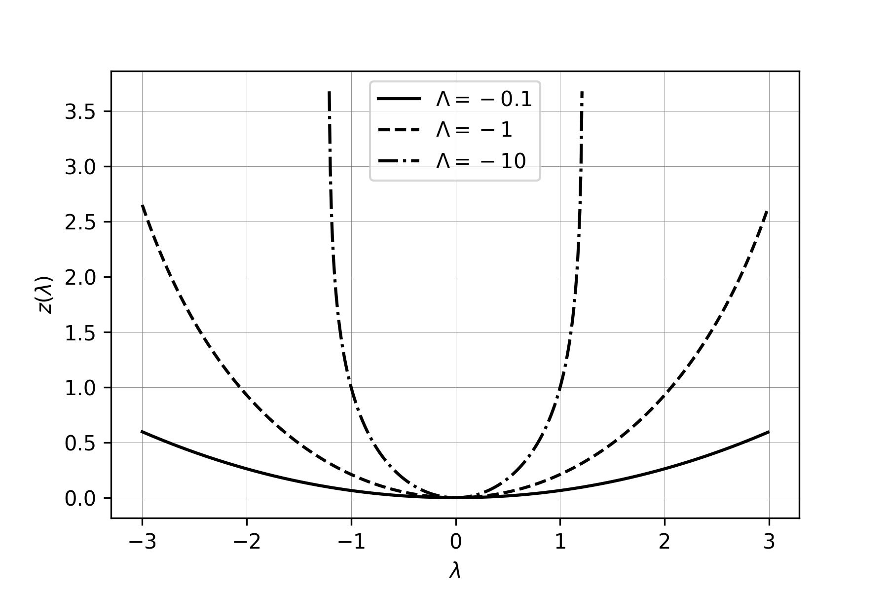
In our model, for each cosmological constant value that we intend to mimic, we have to choose a particular . See this relation in figure (1). To illustrate the particle behavior we use the dynamical equations present in the last section. Following (16) and (17), the plane motion component is
| (22) |
| (23) |
In other words, the speeds and are influenced by coordinate. The transverse motion, which means the motion along the analog extra dimension, is
| (24) |
It is easy to see that
| (25) |
respectively for and . That leads to an attraction to the brane for and a repulsion from the brane for . From this equation, for , the particles get the speed of light. The solution of (25) is given by
| (26) |
Since the analog particles are photons, we could reproduce these initial conditions by sending a light ray perpendicular to direction. If we do that, it is remarkable that the light particles should be dragged or pulled in -direction because of the metamaterial medium. From Fig. (2), we note that light is not confined at , the analog brane region. Also, the particles at any initial position, , are attracted to the origin, but once they reach it, they are repelled from there. Therefore, the plane behaves like a mirror. It is possible to see that sending particles from any , also reflects in the brane region. As a result, particles from one side could not migrate to the other side of the analog brane.
To compare these behaviors and the theoretical motion for free particles at extra dimensions found in Rubakov (2001), we point out the equation
| (27) |
in terms of time-coordinate parameter. Rewriting, (27) in terms the proper-time parameter is possible to show that an equivalence between the behaviors of analogue particles and real massive particles at RS space-times.
III.2 A analog model for thick brane geometry
In thick brane models, we have the warp factor and we have one or more scalar fields defined along the extra-dimension that smooth the brane. Here we show how the thick domain wall could be mimicked with metamaterials. For this proposal, we follow Gremm (2000), where the corresponding warp function and scalar field are
| (28) |
and
| (29) |
where is the AdS-curvature, , and is brane thickness. Using the (19), we find the class of metamaterials that mimic this kind of brane, they are defined by the tensor components
| (30) |
| (31) |
We could simplify the expression (30) by rescaling (12) as . For the same reason, we perform the changes , . As a result, the permittivity components are redefined as
| (32) |
| (33) |
for the metric . This representation means that particles with different masses could be mimicked by changing only the permittivity component. Still, it is remarkable to see the consistency of our model for small ,
| (34) |
that indicates an almost flat analog geometry as it is expected.
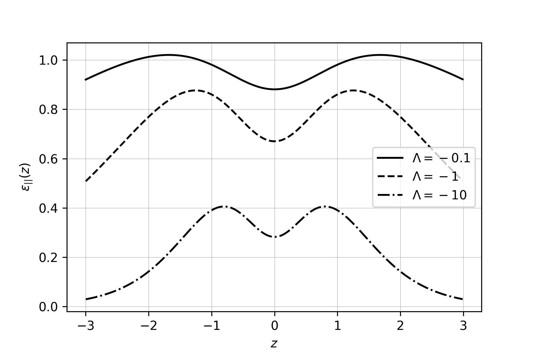
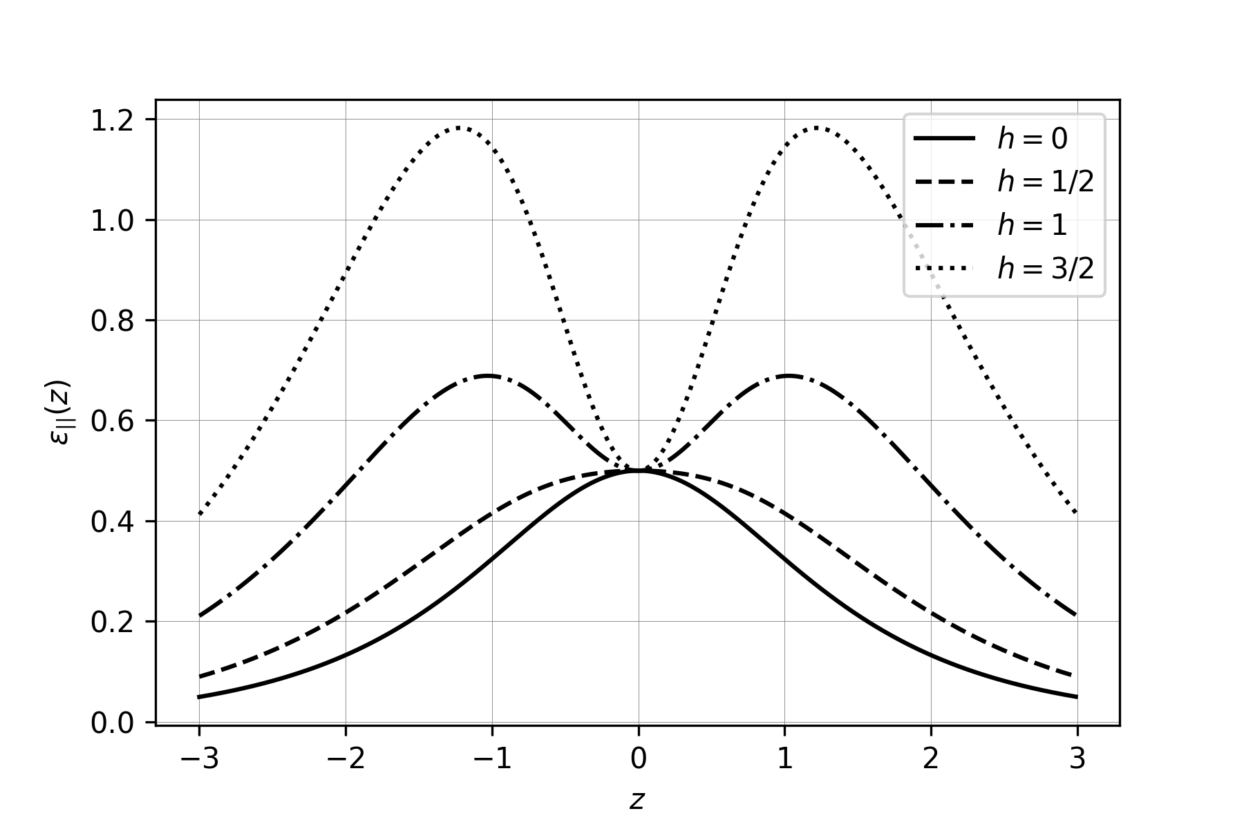
In Fig.(3), we plot (30) without the bar, where we can see a smoothness of the tensor component in comparison with the previous model, fig.(1). This smoothness is also present for different values of analog curvatures and for distinct values at fig.(4).
We can see qualitatively the behavior of particles in the analog branes using the effective potential description,, as defined in Dahia and Romero (2007), with the change . The effective potential becomes
| (35) |
In fact, it could reproduce the same behavior as pointed out in the theory, for different interaction factors . If , there is no stable confinement, as increases the analog particles start to oscillate at the center of the analog brane, which represents the confinement.
IV An analogous asymmetric brane
Metamaterials can be used to simulate asymmetrical brane models. These warp geometries lose the symmetry, as proposed, for example, in Bazeia and Ferreira (2019). They are motivated by cosmological implications Davis et al. (2001), by fermion localization problems Zhao et al. (2010), or even in order to illustrate new braneworld models and its consequences such as gravitational stability Bazeia and Ferreira (2019).
Here we design classes of metamaterials for a particular asymmetrical brane profile Bazeia et al. (2014), where the scalar field and the warp function are
| (36) | |||||
| (37) |
An important feature of this model is the connection of two distinct asymptotically spacetimes, or even the connection of an asymptotically with a Minkowski spacetimes. It is important to state that, in metamaterial research, the junction between two different analog spacetimes had been analysed, as in the case of Minkowski domain walls Smolyaninov and Hung (2013), or in the case of Klein-Minkowski signature transition Figueiredo et al. (2016).
To understand the asymptotic behavior of this model, it is important to note that the warp factor outside of the brane and the five-dimensional cosmological constants,
| (38) |
| (39) |
It is worth noting that some parameters of the model are taken as one, as the brane thickness, for example. In order to mimic the geodesics in this kind of warp geometry, we need a metamaterial with a permittivity tensor governed by
Using and , then
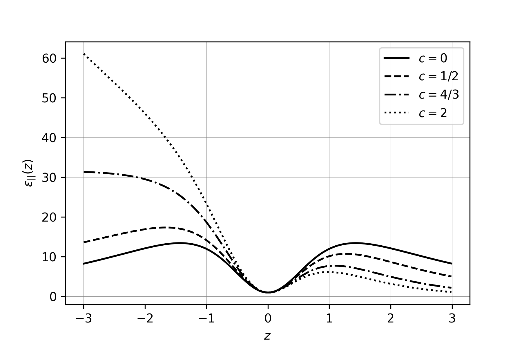
These are the simplified permittivity tensor components. Since the geodesics of and are equivalent, we use the bar metric and we shall write as henceforward. In fig. (5), we can see distinct types of behaviors for . If , it corresponds to a symmetric medium. In the other cases, then, we have asymmetric metamaterials. In fig. (6), we see the permittivity components that mimic the Yukawa-like interaction, and also that breaks the symmetry of the medium.

IV.1 Analog massive particle transverse motion
Here we intend to describe the behavior of analog particles following the analog extra dimension, the direction. The geodesic equation for is , which we can reduce to an autonomous planar dynamical system as follow
| (40) | |||||
| (41) |
where,
| (42) |
From (40) and (41), we can find the critical (equilibrium) points by solving the equations , which implies that all critical points lie on the axis and are located at the roots of (42).
In other words, the set of critical points, , are given by the solutions for . Therefore, let us analyze some cases of interest determined by the values ascribed to the parameters and .
IV.1.1 Case : Analogue bulk
This model was originally proposed in Kehagias and Tamvakis (2001), which has the feature of localized massless chiral fermions. In this case, we still have the symmetry, since the asymmetry parameter is null. The corresponding metamaterials, engineered taking , can realize an asymptotic five-dimensional Anti-de Sitter spacetime, with , in three dimensions.
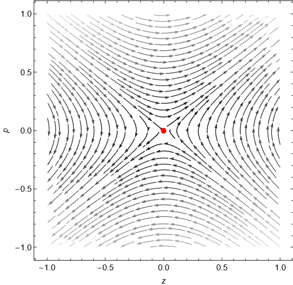
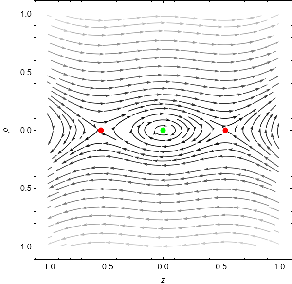
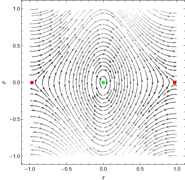
If , then there is only one critical point at the origin of phase space. As already mentioned, the physical role of the parameter is associated with the coupling with the scalar field of the model. Therefore, as this parameter increases, increasing the coupling (or the thickness of the brane), we have the appearance of a region of stability around the origin at the phase space. In this stability region, which grows with the value of , the solutions are represented by orbits in phase space, evidencing a periodic behavior that must be interpreted as mimicking the particle confinement in the brane.
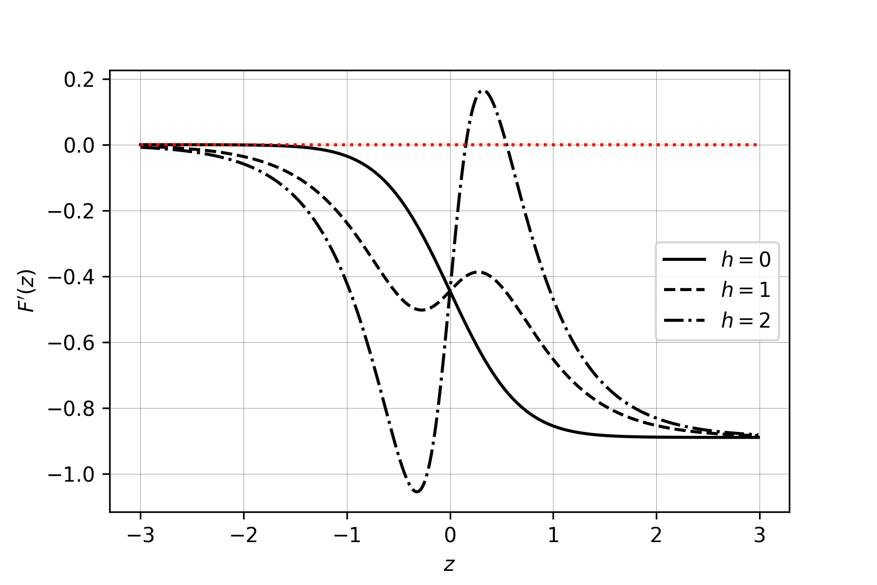
However, when assigning non-zero values to , other roots arise for (42) developing other critical points in the vicinity of the origin. The behavior of (42) for is plotted in Fig.(7).
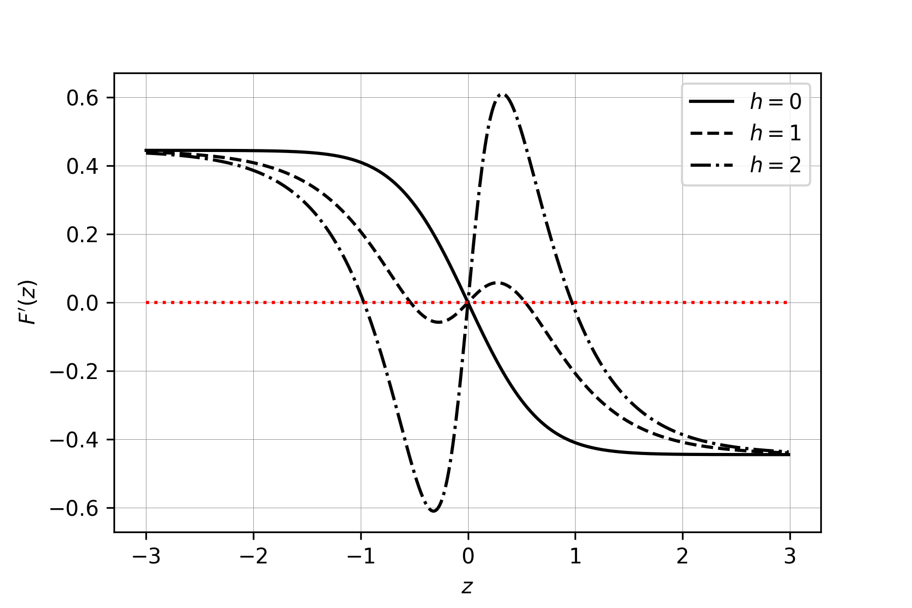
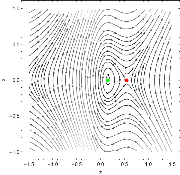
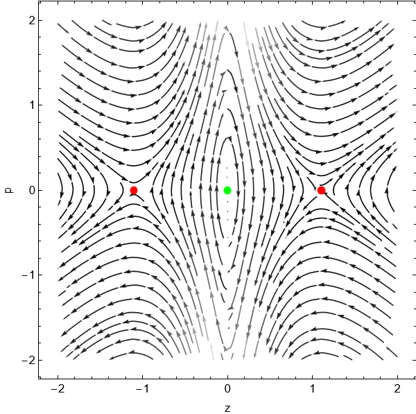
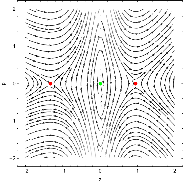
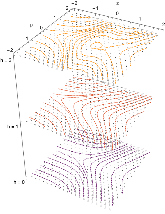
In Fig. (8) we gather the phase portraits for each value of , showing how the behavior of the critical points changes in the case as a function of . For , the analogue particles are reflected from the brane center,. For values the particles are reflected near the saddle points. Also, for , the confinement mechanics make particles oscillate inside the brane, , or oscillate crossing the brane, .
IV.1.2 Case : Analogue Asymmetric bulk
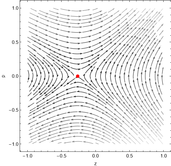
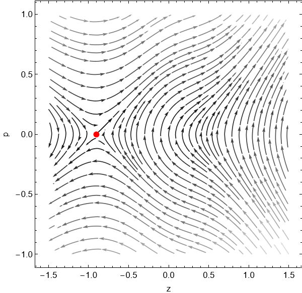
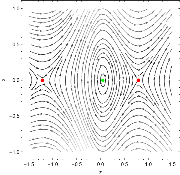
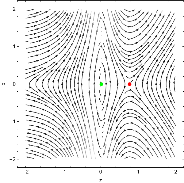
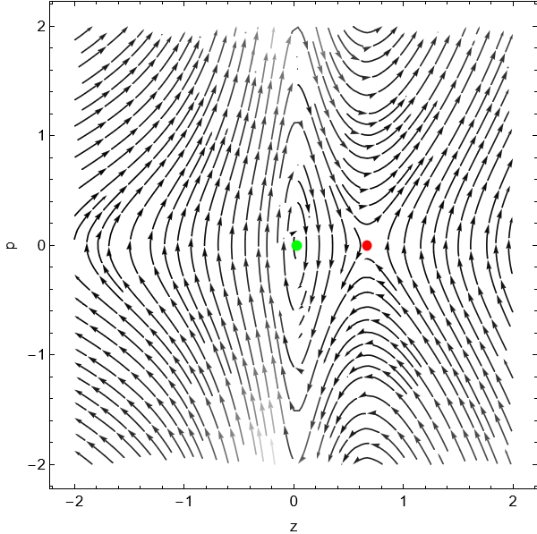
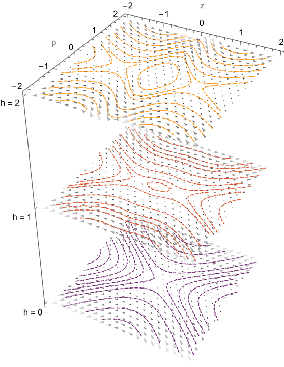
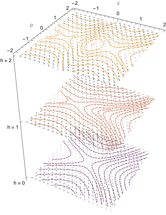
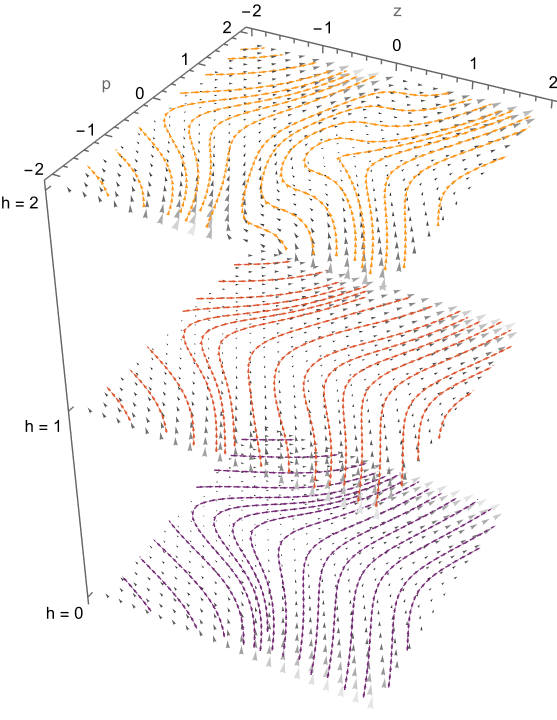
In metamaterials engineered taking , there is a manifestation of the asymmetry of the model. Here, two different asymptotically Anti-de Sitter spacetimes are mimicked, with an analogous as and as . In Fig. (10), we can see the behavior of the geodesics in a phase plot for different parameters.
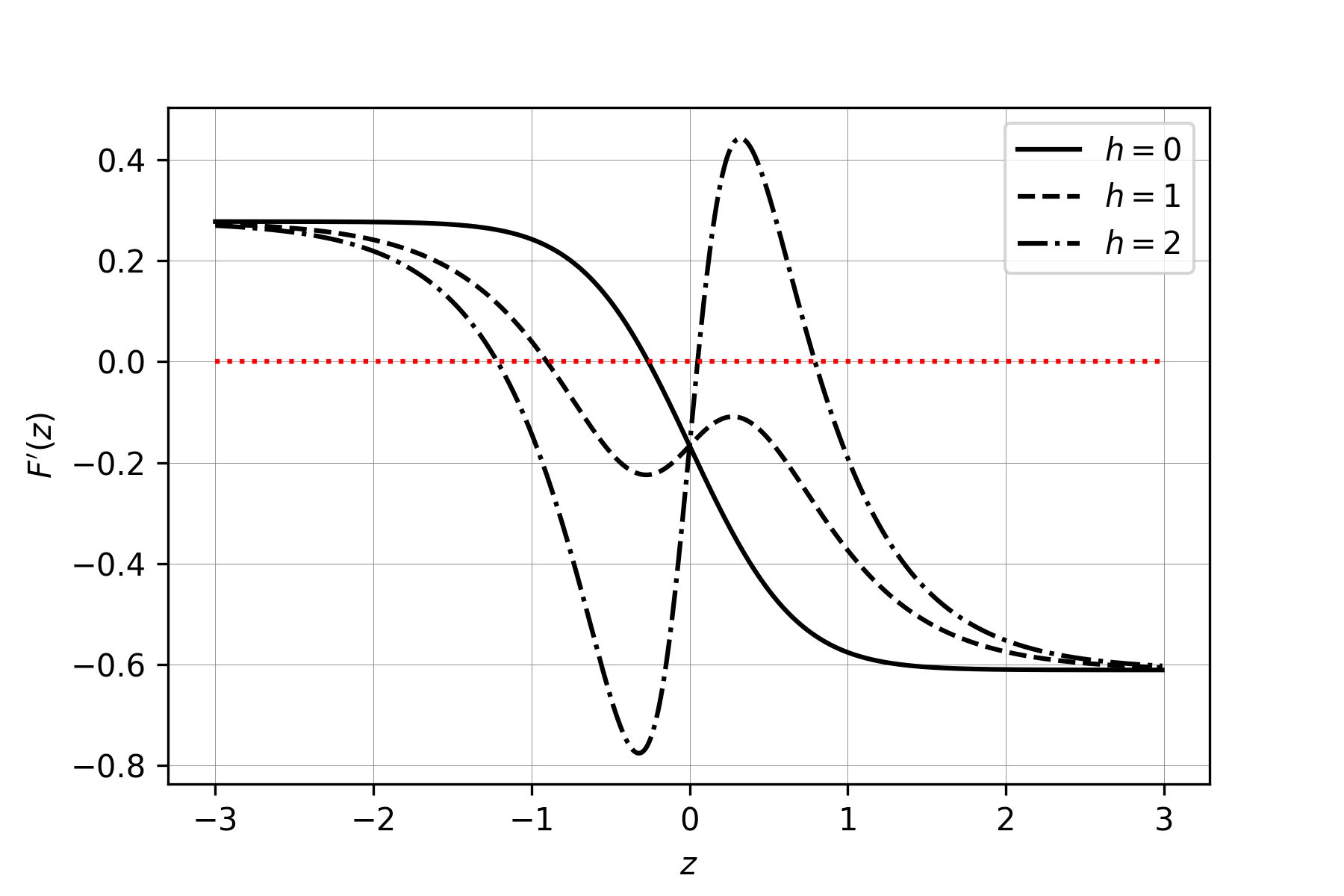
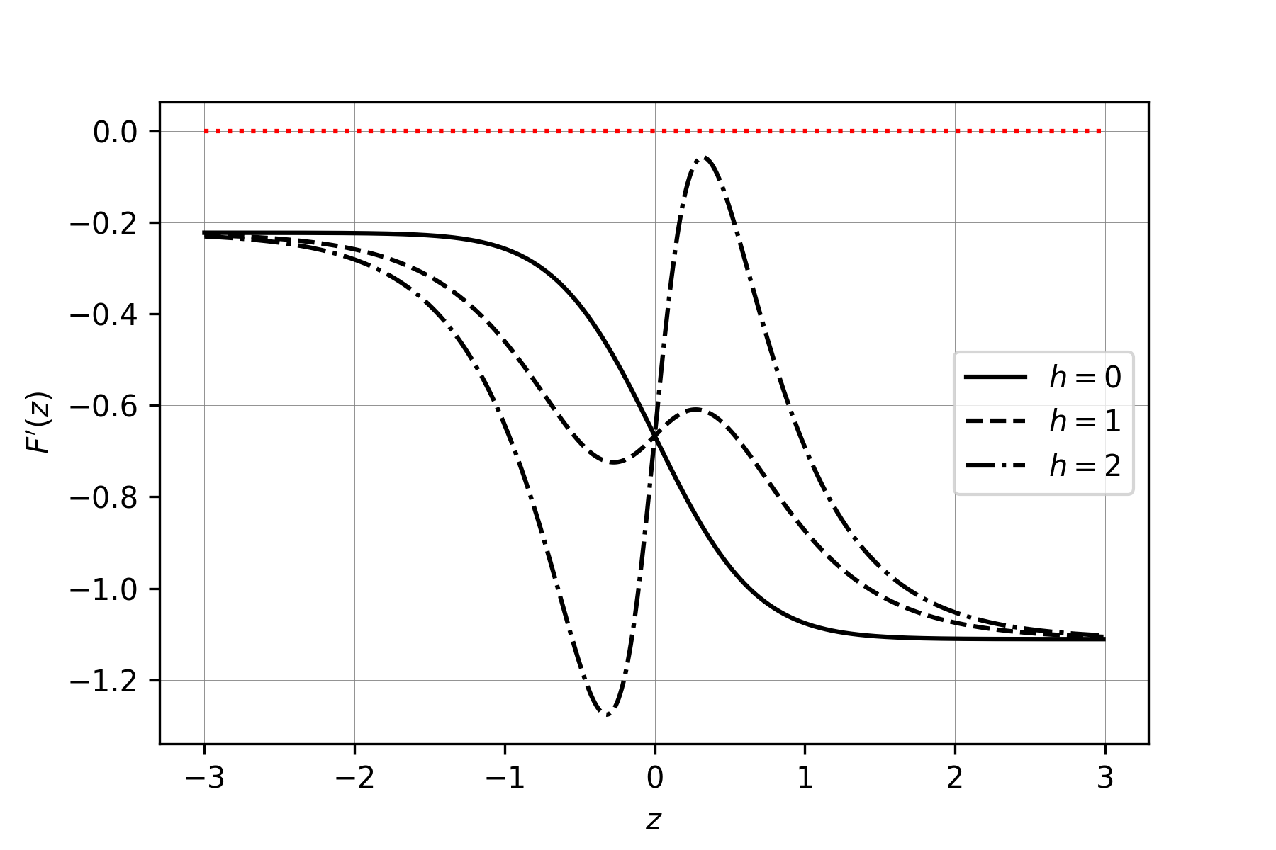
For , there is only one critical point, a saddle point, at the left side, the analog particles are repelled from it. It is also possible, for some restricted conditions, that at this point the particles could be at rest, but this equilibrium is unstable. For , there is still one saddle point. For , two new equilibrium points appear, the stable one is a center near the origin. The number and exact position of the critical points, the roots of , are shown in (9).
Furthermore, if we write an effective potential for this case, following (35), it can be deduced that the analog particles need less energy to go to the right than to go to the left in for all these values. This is a result of the asymmetrical analog bulk.
IV.1.3 Case : An analogue - bulk
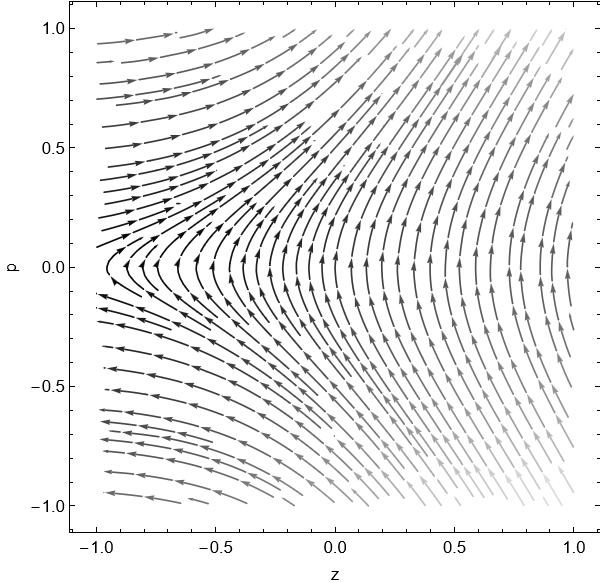
Metamaterials designed with connect an analog Minkowski space-time to an analogue space-time, see Fig. 11 for a few values. As we can see from and also as , this indicates that the analogous on the left side is null. From Fig. 12, it is possible to note that we only have critical points at , one center, and one saddle point, both on the right side. This means that analog particles could be trapped in a tiny region between both of them. Independent of the values, , the light has a tendency to go to the right hand side direction, because they are repelled from the critical point.
IV.1.4 Case : An analogue divergent brane
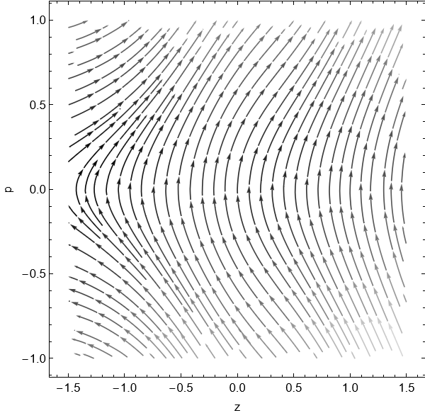
Metamaterials with can simulate a brane model connecting an with to another one with . We can see see that at the left side, the warp factor asymptotically diverges. From the figs. 13 and 14, there is no critical points. Also, we can expect that analog particles at the center should naturally go to the right. There is confinement for higher values of , as (see the Appendix).
IV.1.5 Summary of plots
In summary, we point out some general features of all the phase diagrams here. If , then there is no critical point at the origin as we show in the Appendix. In fact, , such that determines the “repulsion” at the brane center . Particles at rest also moves according to , independent of their positions. Another general feature determined by is the asymptotic behavior, as then . In this brane description, we use positive values for , however, it is possible to construct analog warp geometry models for negative values.
V Conclusion
In this article, we show profiles of materials that can mimic the geodesics of massive particles in some braneworld models, with and without the confinement mechanism of bosonic particles. It is known that there are other mechanisms of confinement in the literature Souza et al. (2021), however, it requires more study in order to design metamaterials for them.
In metamaterials modeled with (19), in the case of analogue thick branes, the light ray particles get an associated analog mass that depends on the metamaterial parameters. Then, particles with different masses can not be represented by the same medium. As a consequence, we cannot simulate the split particles in different slices of the brane as it could occur for fermions according to Dahia et al. (2013).
In order to map a photon, we could use a hyperbolic liquid crystal metamaterial. Given the line element , where we associate the coordinate with the extra-dimension, and and to coordinates in the brane. Choosing and . We easily get that massless particles move according to the equations and , where is a constant of the motion. Therefore, the photon motion in the direction is given by and for radial emission, , the equation gets the form , that simulates the transverse motion along the extra-dimension, according to (11).
Concerning the asymmetrical analog brane, we find that light could stop at the saddle points. This seems to have a connection with slow light phenomena, however according to Reza et al. (2008) this should not happen, and as a consequence, we need the electromagnetic wave approach to understand better this issue. Still, we can infer general features for our models from our results. Since the metric (12)is valid and is constant, then at a critical point, we have that the confinement is possible, however, if at the critical point, then there is no confinement of light at this region.
Finally, it seems to us, that our proposals could be adapted to study the geodesic motion in bi-dimensional sub-manifolds of six-dimensional space-time warp geometries such as the Gergheta-Shaposhnikov or string-cigar models Gherghetta and Shaposhnikov (2000); Silva et al. (2012); Costa et al. (2015), where the two new co-dimensions are and . Furthermore, since there are few results in the extra-dimensional analog models, for example Barceló and Campos (2003), we expect to shed light on Randall-Sundrum like models at the lab.
Acknowledgements.
We would like to thank C. Romero and F. Dahia for their helpful discussions. This work was supported by Conselho Nacional de Desenvolvimento Científico e Tecnológico (CNPq), grants Nos. 150480/2021-0 (ABB) and 311798/2021-7 (FM).References
- Wesson (2006) P. S. Wesson, Five-dimensional physics: classical and quantum consequences of Kaluza-Klein cosmology (World Scientific, 2006).
- Arkani-Hamed et al. (1998) N. Arkani-Hamed, S. Dimopoulos, and G. Dvali, Physics Letters B 429, 263 (1998).
- Mannheim (2005) P. D. Mannheim, Brane-localized gravity (World Scientific, 2005).
- Weinberg (1989) S. Weinberg, Reviews of modern physics 61, 1 (1989).
- Fitzpatrick et al. (2008) A. L. Fitzpatrick, G. Perez, and L. Randall, Physical review letters 100, 171604 (2008).
- Feruglio (2004) F. Feruglio, The European Physical Journal C-Particles and Fields 33, s114 (2004).
- Randall and Sundrum (1999a) L. Randall and R. Sundrum, Physical Review Letters 83, 4690 (1999a).
- Randall and Sundrum (1999b) L. Randall and R. Sundrum, Physical review letters 83, 3370 (1999b).
- Felder et al. (2002) G. N. Felder, A. V. Frolov, and L. Kofman, Class. Quant. Grav. 19, 2983 (2002), arXiv:hep-th/0112165 .
- Kretzschmar et al. (2016) J. Kretzschmar et al., Nuclear and particle physics proceedings 273, 541 (2016).
- Dahia and Lemos (2016a) F. Dahia and A. Lemos, The European Physical Journal C 76, 1 (2016a).
- Wang and Ni (2013) L.-B. Wang and W.-T. Ni, Modern Physics Letters A 28, 1350094 (2013).
- Dahia and Lemos (2016b) F. Dahia and A. Lemos, Physical Review D 94, 084033 (2016b).
- Lemos et al. (2019) A. Lemos, G. Luna, E. Maciel, and F. Dahia, Classical and Quantum Gravity 36, 245021 (2019).
- Jacobson (1991) T. Jacobson, Physical Review D 44, 1731 (1991).
- Drori et al. (2019) J. Drori, Y. Rosenberg, D. Bermudez, Y. Silberberg, and U. Leonhardt, Physical Review Letters 122, 010404 (2019).
- Barceló et al. (2011) C. Barceló, S. Liberati, and M. Visser, Living reviews in relativity 14, 1 (2011).
- Figueiredo et al. (2016) D. Figueiredo, F. A. Gomes, S. Fumeron, B. Berche, and F. Moraes, Physical Review D 94, 044039 (2016).
- Alves-Júnior et al. (2021) F. Alves-Júnior, A. Barreto, and F. Moraes, Physical Review D 103, 044023 (2021).
- Smolyaninov and Narimanov (2010) I. I. Smolyaninov and E. E. Narimanov, Physical Review Letters 105, 067402 (2010).
- Fernández-Núñez and Bulashenko (2016) I. Fernández-Núñez and O. Bulashenko, Physics Letters A 380, 1 (2016).
- Azevedo et al. (2021) F. d. S. Azevedo, J. D. M. de Lima, A. de Pádua Santos, and F. Moraes, Physical Review A 103, 023516 (2021).
- Fernández-Núñez and Bulashenko (2018) I. Fernández-Núñez and O. Bulashenko, Journal of Optics 20, 045603 (2018).
- Leonhardt and Philbin (2009) U. Leonhardt and T. G. Philbin, in Progress in optics, Vol. 53 (Elsevier, 2009) pp. 69–152.
- Rho et al. (2013) J. Rho, X. Yang, J. Yao, X. Yin, and X. Zhang, in CLEO: 2013 (Optica Publishing Group, 2013) p. JTu4A.78.
- Chen et al. (2010) H. Chen, C. T. Chan, and P. Sheng, Nature materials 9, 387 (2010).
- Quach et al. (2013) J. Q. Quach, C.-H. Su, and A. D. Greentree, Opt. Express 21, 5575 (2013).
- Smolyaninov (2010) I. I. Smolyaninov, Journal of Optics 13, 024004 (2010).
- Dahia and Romero (2007) F. Dahia and C. Romero, Physics Letters B 651, 232 (2007).
- La Camera (2008) M. La Camera, Modern Physics Letters A 23, 2727 (2008).
- Romero et al. (2011) C. Romero, J. Formiga, and C. Dariescu, Gravitation and Cosmology 17, 252 (2011).
- Guha and Chakraborty (2010) S. Guha and S. Chakraborty, General Relativity and Gravitation 42, 1739 (2010).
- Ghosh et al. (2010) S. Ghosh, S. Kar, and H. Nandan, Physical Review D 82, 024040 (2010).
- Dahia et al. (2007) F. Dahia, L. F. da Silva, C. Romero, and R. Tavakol, Journal of mathematical physics 48, 072501 (2007).
- Dahia et al. (2008) F. Dahia, C. Romero, L. F. da Silva, and R. Tavakol, General Relativity and Gravitation 40, 1341 (2008).
- Dzhunushaliev et al. (2010) V. Dzhunushaliev, V. Folomeev, and M. Minamitsuji, Reports on Progress in Physics 73, 066901 (2010).
- Mück et al. (2000) W. Mück, K. Viswanathan, and I. Volovich, Physical Review D 62, 105019 (2000).
- Rubakov (2001) V. A. Rubakov, Physics-Uspekhi 44, 871 (2001).
- Gremm (2000) M. Gremm, Physics Letters B 478, 434 (2000).
- Bazeia and Ferreira (2019) D. Bazeia and D. Ferreira, Annals of Physics 411, 167975 (2019).
- Davis et al. (2001) A.-C. Davis, I. Vernon, S. C. Davis, and W. B. Perkins, Physics Letters B 504, 254 (2001).
- Zhao et al. (2010) Z.-H. Zhao, Y.-X. Liu, and H.-T. Li, Classical and Quantum Gravity 27, 185001 (2010).
- Bazeia et al. (2014) D. Bazeia, R. Menezes, and R. da Rocha, Advances in High Energy Physics 2014 (2014).
- Smolyaninov and Hung (2013) I. I. Smolyaninov and Y.-J. Hung, Physics Letters A 377, 353 (2013).
- Kehagias and Tamvakis (2001) A. Kehagias and K. Tamvakis, Physics Letters B 504, 38 (2001).
- Souza et al. (2021) F. Souza, G. Alencar, L. Freitas, and R. Landim, Europhysics Letters 133, 50001 (2021).
- Dahia et al. (2013) F. Dahia, A. d. A. Silva, and C. Romero, arXiv preprint arXiv:1311.4751 (2013).
- Reza et al. (2008) A. Reza, M. Dignam, and S. Hughes, Nature 455, E10 (2008).
- Gherghetta and Shaposhnikov (2000) T. Gherghetta and M. Shaposhnikov, Physical Review Letters 85, 240 (2000).
- Silva et al. (2012) J. E. G. Silva, V. Santos, and C. Almeida, Classical and Quantum Gravity 30, 025005 (2012).
- Costa et al. (2015) F. W. V. d. Costa, J. E. G. d. Silva, D. F. d. S. Veras, and C. A. S. d. Almeida, Physics Letters B 747, 517 (2015).
- Barceló and Campos (2003) C. Barceló and A. Campos, Physics Letters B 563, 217 (2003).
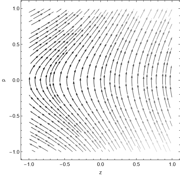
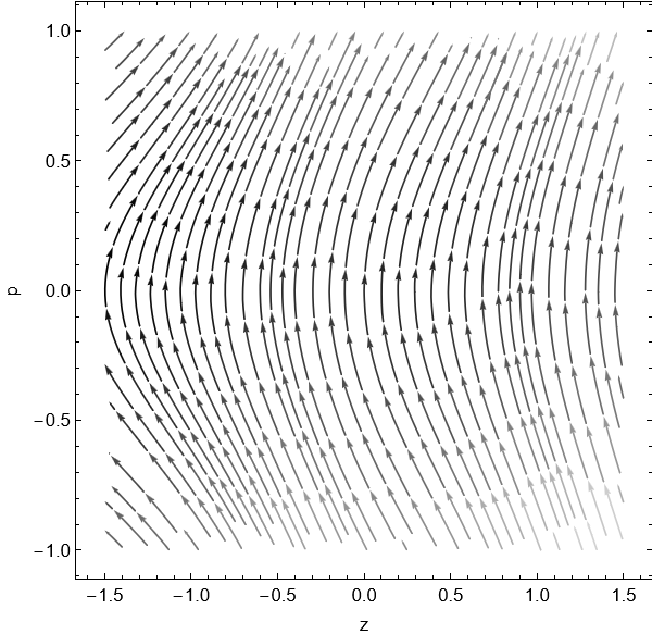
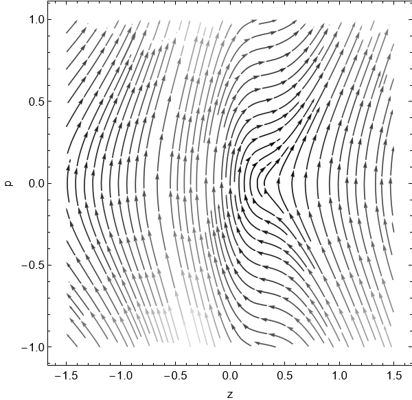
Appendix A Phase portraits
Here we present some additional phase portraits of the dynamical system defined by Eqs. (40) and (41) of the analog asymmetrical branes (section ), for some values of and . Where they appear, the red dots represent saddle points (unstable), and the green dots, centers (stable).