Email: ]wsengupta@princeton.edu

Periodic Korteweg-de Vries soliton potentials generate magnetic field strength with exact quasisymmetry

Abstract

Quasisymmetry (QS) is a hidden symmetry of the magnetic field strength, $|\mathbf{B}|$, that confines charged particles effectively in a nonsymmetric toroidal plasma equilibrium. Recent numerical breakthroughs have shown that excellent QS can be realized in a toroidal volume. Here, we show that the hidden symmetry of QS has a deep connection to the underlying symmetry that makes solitons possible. In particular, we demonstrate that a class of quasisymmetric $|\mathbf{B}|$ is described by a periodic finite-gap soliton potential of the well-known Korteweg-de Vries (KdV) equation. Our exact and non-perturbative method drastically reduces the number of independent $|\mathbf{B}|$ parameters on a magnetic flux surface to just three, which could make stellarator optimization schemes significantly more efficient. Furthermore, we deduce an upper bound on the maximum toroidal volume that can be quasisymmetric. In the neighborhood of the outermost surface, $|\mathbf{B}|$ approaches the form of the 1-soliton reflectionless potential.

Physical systems possessing hidden symmetries (HS) attract serious attention Charalambous, Dubovsky, and Ivanov (2021); Lee et al. (2021); Liu and Tegmark (2022); Landreman and Paul (2022); Moser (1979); Leach and Andriopoulos (2008) because of the far-reaching impact of the symmetry on the physical properties of the systems. HS manifests only in special coordinates, which are constructed, along with the invariants, as part of the solution to the problem. In the presence of HS, the partial differential equations (PDEs) governing classical dynamical fields often reduce to integrable PDEs. (Moser, 1979; Ovsienko and Khesin, 1987; Leach and Andriopoulos, 2008) An example of the latter is the well-known Korteweg-de Vries (KdV) equation with soliton solutions.Gardner et al. (1967); Novikov et al. (1984)

An analogous and well-studiedLewis Jr (1967); Leach and Andriopoulos (2008); Gjaja and Bhattacharjee (1992) mechanical example of HS occurs in the one-dimensional time-dependent harmonic oscillator problem, which can be shown to admit the so-called Ermakov-Lewis invariant (ELI). The ELI is the action variable for the harmonic oscillator. The symmetry that leads to the ELI is nontrivial Leach and Andriopoulos (2008) and related to that underlying the KdV.Brezhnev (2008); Leach and Andriopoulos (2008) Furthermore, for soliton (or reflectionless) potentials, the adiabatic invariants obtained using the eikonal (Wentzel-Kramers-Brillouin or WKB) approximation become exact invariants. (Gjaja and Bhattacharjee, 1992; Berry and Howls, 1990)

In plasma physics, a hidden symmetry called quasisymmetry (QS), (Boozer, 1983; Helander, 2014) forces the magnetic field strength, $B=|\mathbf{B}|$, to be symmetric,(Boozer, 1983; Rodriguez, 2022) whereas B itself is fully three-dimensional (3D). Several practical reasons exist for building 3D toroidal magnetic confinement fusion devices called stellarators with quasisymmetric $B$. The HS in $B$ makes the bounce action (second adiabatic invariant), $J_{||}$, independent of the field-line label,(Helander, 2014) which guarantees excellent particle confinement on a torus. The 3D nature of B allows stellarators to avoid intrinsic difficulties (such as powerful transients) associated with large plasma currents. (Helander, 2014)

It is currently unknown whether QS can be achieved exactly in a toroidal volume for a magnetic field that satisfies the constraint of force-balance in ideal magnetohydrodynamics (MHD).Freidberg (2014)(Burby, Kallinikos, and MacKay, 2020; Helander, 2014; Plunk and Helander, 2018; Garren and Boozer, 1991a, b) Analytical results (Garren and Boozer, 1991a, b; Plunk and Helander, 2018; Landreman and Sengupta, 2019) seem to indicate that in the presence of scalar plasma pressure, the resulting 3D nonlinear system of PDEs is overdetermined and does not have solutions in a toroidal volume.(Garren and Boozer, 1991a, b; Landreman and Sengupta, 2019; Constantin, Drivas, and Ginsberg, 2021; Rodríguez, Helander, and Bhattacharjee, 2020; Rodríguez, Sengupta, and Bhattacharjee, 2022) In particular, the near-axis expansion (NAE),(Garren and Boozer, 1991a, b; Landreman and Sengupta, 2018) an asymptotic expansion in the distance from the magnetic axis, is typically divergent beyond the second-order. On the other hand, designs with a precise level of QS and MHD force balance have been obtained through large-scale numerical optimization, hinting at the possible existence of special solutions to the overdetermined problem.

Further analytical insight into these unique configurations that approximately solve the overdetermination problem is needed. In the special case of isodynamic magnetic fields, which satisfy a constraint more restrictive but related to QS,(Helander, 2014; Schief, 2003) the soliton solutions(Schief, 2003) of the vortex filament equations play a significant role. However, the overdetermination problem for QS is more complicated than that for isodynamic fields. Hence we focus on the functional form of QS magnetic field strength without enforcing a force-balance condition. Our motivation here is to study the possible connections between QS and other HS with an invariant, such as the ELI,Leach and Andriopoulos (2008); Gjaja and Bhattacharjee (1992) analogous to the field-line label independence of $J_{||}$.

In this Letter, starting from the basic definitions and properties of QS, we show non-perturbatively that QS admits a class of analytic $B$ that is a periodic solution(Novikov et al., 1984; Kamchatnov, 2000) of the KdV equation. The exact analytic solution for $B$ is valid in a toroidal volume and is consistent with the NAE predictions close to the magnetic axis. The connection with periodic KdV solitons allows us to describe $B$ on a magnetic flux surface with only three functions of the magnetic flux, related to the so-called “spectral parameter”(Novikov et al., 1984) of the KdV. We show that these functions are closely related to the spectrum of $B$ in Boozer coordinates Helander (2014) where the HS is manifest, thereby highlighting the low dimensionality of the Boozer spectrum. Furthermore, our analysis shows that the periodicity of $B$ is maintained only when these functions are distinct. Consequently, we can estimate the region of validity of volumetric quasisymmetry based on where the two spectral parameters intersect (shown below). Remarkably, near the point of intersection, the connection length (period of $B$) begins to diverge, and $B$ approaches the form of a reflectionless potential (a single soliton that decays at infinity). We demonstrate that our analytic theory can describe a vacuum equilibrium with precise quasi-axisymmetry (QA)Landreman and Paul (2022) and many other numerically-optimized quasisymmetric configurations.

We begin by reviewing some of the known basic properties of QS. We enforce QS through the condition (Freidberg, 2014)

$$\frac{\partial B}{\partial\ell}=f(B;\psi),$$ (1)

which is equivalent to the “triple-product” form of QS.(Rodriguez, 2022; Rodríguez, Helander, and Bhattacharjee, 2020) Moreover, due to the toroidal setting, $B$ is subject to the following periodic boundary condition (Helander, 2014)

$$B(\psi,\alpha,\ell)=B(\psi,\alpha,\ell+L(\psi)).$$ (2)

Here, $(\psi,\alpha,\ell)$ is the standard Clebsch coordinate system such that $\bm{B}=\bm{\nabla}\psi\times\bm{\nabla}\alpha$,Helander (2014) with flux label $\psi$, field-line label $\alpha$, and $\ell$, the arclength along the magnetic field. Since $\alpha$ is a multi-valued function, we impose suitable toroidal cuts. The period of $B$, $L(\psi)$, is called the connection length and is a quantity of great physical interest. In terms of the translation operator $T$ such that $Tf(\ell)=f(\ell+L)$, the periodic boundary condition can be written $TB=B$. In addition, (1) implies Freidberg (2014) that

$$\frac{\partial B}{\partial\alpha}+H(\psi,\alpha)\frac{\partial B}{\partial\ell}=0,$$ (3)

where $H(\psi,\alpha)$ is independent of $\ell$ and depends on the definition of the origin of $\ell$. There is a considerable degree of freedom in choosing $H$. For example, by redefining $\ell\mapsto\ell-\int d\alpha H(\psi,\alpha)$, we can reduce (3) to $\partial_{\alpha}B=0$.(Freidberg, 2014) Furthermore, because of (1), any integral along the magnetic field line between two points of equal values of $B=B_{b}$ satisfies

$$\partial_{\alpha}\int_{B\leq B_{b}}d\ell\;F(B;\psi)=0.$$ (4)

Omnigeneous magnetic fields, Helander (2014) in contrast with quasisymmetric ones, satisfy (4) but not (2).

We now address the central problem of this Letter. We shall consider the quasisymmetric system (1), (2), and (3) as a PDE system on a constant flux surface $\psi$. We will define a time-like variable, $t\propto\int H(\psi,\alpha)d\alpha$, and a space-like variable, $x\propto l$, where both proportionality factors depend only on $\psi$. The fundamental problem is to find periodic time-dependent $B(\ell,t;\psi)$ that support time-independent integrals that obey (4). In particular, we shall focus on PDEs with exact ELI.

In our search for a special $B$ that has an exact invariant, we are led to the ELI (or equivalently Courant-Snyder Courant and Snyder (1958)) theory. Leach and Andriopoulos (2008); Lewis Jr (1967); Gjaja and Bhattacharjee (1992) A harmonic oscillator with a variable frequency, $\omega^{2}(\ell,t)\equiv\mathcal{E}-B(\ell,t),$ possesses the nontrivial exact ELI, $I(\mathcal{E})$. The oscillator equation (Brezhnev, 2008; Gjaja and Bhattacharjee, 1992) is nothing but the time-independent Schrodinger equation (SE)

$$\mathcal{L}\Psi=\mathcal{E}\Psi,\quad\mathcal{L}\equiv(-\partial_{\ell}^{2}+B(\ell,t;\psi)),$$ (5)

with $B$ as a potential and $\mathcal{E}$, a real constant. The exact solution to the SE (5) is of the form $\Psi_{\pm}=\rho\exp{i\chi_{\pm}}$, where $\chi_{\pm}=\pm\sqrt{2I}\int d\ell/\rho^{2}$, and $\rho$ satisfies the nonlinear Ermakov-Pinney Leach and Andriopoulos (2008); Brezhnev (2008) equation

$$(\partial_{\ell}^{2}+(\mathcal{E}-B))\rho=2I(\mathcal{E})/\rho^{3}.$$ (6)

Moreover, since $B$ is periodic in $\ell$, the Floquet-Bloch theorem Magnus and Winkler (2013); Novikov et al. (1984); Kamchatnov (2000) guarantees that there exists simultaneous eigenfunctions, $\Psi_{\pm}$, such that

$$\mathcal{L}\Psi_{\pm}=\mathcal{E}\Psi_{\pm},\quad T\Psi_{\pm}=e^{\pm i\mathfrak{p}L}\Psi_{\pm},$$ (7)

where $\mathcal{E}$ is now called the spectral parameter. The Floquet multiplier, $\mathfrak{p}(\mathcal{E})$, also known as the quasimomentum, Novikov et al. (1984) is given by $\pm\mathfrak{p}(\mathcal{E})L=\oint d\ell\chi_{R}$, where $\chi_{R}$ is the real part of $\chi_{\pm}$. Thus $\mathfrak{p}(\mathcal{E})$ is an exact invariant and is proportional to $\sqrt{2I(\mathcal{E})}$.

The SE (5) enjoys a special connection with soliton theory since it is also one of the Lax pairs,Gardner et al. (1967); Lax (1968); Novikov et al. (1984) for the KdV equation, (Kamchatnov, 2000; Novikov et al., 1984)

$$\frac{\partial B}{\partial t}+6B\frac{\partial B}{\partial x}+\frac{\partial^{3}B}{\partial x^{3}}=0.$$ (8)

The fundamental idea behind Lax pairs Lax (1968); Tao (2009) is that most integrable nonlinear systems can be obtained as a consistency condition of the overdetermined linear system

$$L\Psi=\mathcal{E}\Psi,\quad\partial_{t}\Psi=P\Psi,$$ (9)

where $L,P$ are linear operators. The isospectral ($\partial_{t}\mathcal{E}=0$) consistency condition of the system (9), given by the Lax equation,

$$\partial_{t}L=[P,L],$$ (10)

then leads to an integrable nonlinear PDE. The choice of the Schrodinger operator as a Lax pair, i.e., $L=\mathcal{L}$, together with suitable choices for $P$, leads to the KdV hierarchy.Novikov et al. (1984) Since the evolution is isospectral, the quasimomentum $\mathfrak{p}(\mathcal{E})$ remains independent of time if $B(\ell,t,\psi)$ evolves under KdV. Moreover, the Lax equation guarantees an infinite number of conserved quantities of the form (4). We note that the periodicity condition, together with the Lax equation, imposes severe restrictions Gesztesy and Weikard (1996); Dubrovin, Krichever, and Novikov (1990) on the choice of $P,L$. Consequently, the Floquet-Bloch spectrum can be shown to have only a finite number of gaps.Novikov et al. (1984); Brezhnev (2008)

With these results from soliton theory in mind, let us now turn to the QS problem. As discussed earlier, a special finite-gap potential $B$, which solves KdV, is guaranteed to have invariants (4) and the ELI, $I$. However, to gain physical insight, we shall now consider the WKB limit of the SE (5) for $\Psi_{\pm}$. In the WKB approach, we obtain $\chi_{\pm}\approx\pm\sqrt{\mathcal{E}-B}$. Froman (1979), from which it follows that $\pm\mathfrak{p}L=\oint d\ell\chi_{R}$ is the adiabatic invariant $J_{||}$

$$J_{||}=\oint\sqrt{\mathcal{E}-B}\;d\ell.$$ (11)

Here we have interpreted $\mathcal{E}$ to be related to the particle energy. Since only the real part of $\chi_{\pm}$ is involved, integration is performed in the region $\mathcal{E}-B\geq 0$. Therefore, both passing and trapped orbits Helander (2014); Froman (1979) are accounted for. From the QS condition (4), it then follows that $J_{||}$, and in general, $\mathfrak{p}(\mathcal{E})$ given by (7), are time-independent. Furthermore, for passing orbits, an alternative approach based on a large $\mathcal{E}$ limit Novikov et al. (1984) shows that $\mathfrak{p}(\mathcal{E})$ generates the infinite hierarchy of time-independent KdV integrals that are polynomials in $B$ and its derivatives, and satisfy (4).

Noting the relation between the KdV and QS invariants, we now consider the consistency between the QS conditions (1)-(3) and the KdV equations. The structure of equation (3) suggests that the search for a quasisymmetric $B$ can be further restricted to traveling wave solutions of the KdV equation, i.e., $B=B(\ell-\int d\alpha H(\psi,\alpha))$. The equation obtained from the KdV equation by first moving to the traveling wave frame and integrating twice Kamchatnov (2000) is indeed of the form (1) with the function $f(B;\psi)$ being a cubic function of $B$, that is,

$$\left(\frac{\partial B}{\partial\ell}\right)^{2}=\mathcal{D}(\psi)(B_{M}-B)(B-B_{m})(B-B_{X}),$$ (12)

where the roots of the cubic polynomial, $B_{i}=\{B_{M},B_{m},B_{X}\}$, are functions of $\psi$, and $\mathcal{D}(\psi)$ is a proportionality factor. The exact solution of (12) subject to the periodicity constraint (2) can be expressed in terms of elliptic functions.(Kamchatnov, 2000; Novikov et al., 1984) Thus, we have shown that $B$ given by a periodic traveling wave solution of the KdV equation meets the QS requirements (1)-(4).

Note that the QS constraints by themselves are not sufficient to restrict the form of the arbitrary function $f(B;\psi)$ in the $\partial B/\partial\ell$ equation (1) to a simple cubic in (12). However, if we make the connection between the QS invariants and the ELI, the cubic relation follows from periodicity (2) and the isospectral (Lax) condition (10).

To obtain the proportionality factors between $(x,t)$ and $(l,\alpha)$ explicitly, we now proceed from (12) and derive the KdV equation. Differentiating (12) twice with $\ell$ and using the $\partial_{\alpha}B$ equation (3) we get (8), the KdV equation for $B$. Here, the coordinates $(x,t)$ are defined in terms of $(\alpha,\ell)$ as

$$\frac{x}{\ell}=\sqrt{\frac{\mathcal{D}}{2}},\;\;\frac{t}{\int d\alpha H}=\frac{\sqrt{\mathcal{D}/2}}{2(B_{M}+B_{m}+B_{X})}.$$ (13)

The $\partial_{\alpha}B$ relation (3), now takes the following form of a 1D traveling wave equation with speed $c(\psi)$,

$$\frac{\partial B}{\partial t}+c(\psi)\frac{\partial B}{\partial x}=0,\quad c(\psi)=2(B_{M}+B_{m}+B_{X}).$$ (14)

$B$ is then obtained from the cnoidal solution (Kamchatnov, 2000) of KdV,

$$B =B_{m}+(B_{M}-B_{m})\text{cn}^{2}\left(\sqrt{\frac{B_{M}-B_{X}}{2}}(x-ct),m\right),$$

$$m =\frac{B_{M}-B_{m}}{B_{M}-B_{X}},\quad 0\leq m\leq 1.$$ (15)

Here, $\text{cn}(u,m)$ is the Jacobi cosine elliptic function with modulus $m$. $B$ varies between $B_{m}$ and $B_{M}$. The period of $B$, $L(\psi)$, diverges logarithmically as $m\to 1$. One would expect this behavior near a separatrix, where periodicity along a field line is lost because the field line cannot cross the X-point. In particular, it is interesting to note that in the $m\to 1$ limit, $B$ takes the form of the infinite KdV soliton (reflectionless potential).

The connection with KdV significantly reduces the dimensionality of this class of quasisymmetric $B$. We first note that on any flux surface $\psi$, we have four flux functions that determine $B$, namely $\mathcal{D}$ and $B_{M},B_{m},B_{X}$, the three real roots of the cubic polynomial in (12). However, as shown in Appendix A $\mathcal{D}$ can be expressed in terms of the rotational transform $\iota$ and the roots. Therefore, the connection with KdV points to a hidden low-dimensionality of the description of $B$.

The functions $B_{M}$ and $B_{m}$ denote the values of $B$ on a flux surface at the maxima and minima, and $B_{X}$ is a third root of the polynomial. The behavior of $B$ in Boozer coordinates is well known (Garren and Boozer, 1991a, b; Landreman and Sengupta, 2018) near the magnetic axis and is consistent with (12). On the axis $B$ is a constant, $B_{0}$, and varies as $B\approx B_{0}(1+\overline{\eta}\sqrt{2\psi}\cos\vartheta)+2\psi(B_{20}+B_{22}\cos 2\vartheta)$ near the axis. Here, $\vartheta$ is the well-known Boozer angle.(Landreman and Sengupta, 2018) The constant $\overline{\eta}$ dominates the maximum variation of $B$ on a flux surface, with the $O(2\psi)$ term being only a small second-order correction. Within the NAE framework, $B_{X}$ and $\mathcal{D}$ are constant throughout the volume, with $\mathcal{D}\propto((\iota-N/M))^{2}$. The NAE predicts

$$\frac{B_{M}}{B_{0}},\frac{B_{m}}{B_{0}}=1\pm\overline{\eta}\sqrt{2\psi},\quad\frac{B_{X}}{B_{0}}=\frac{4B_{22}/B_{0}+\overline{\eta}^{2}}{4B_{22}/B_{0}+2\overline{\eta}^{2}}.$$ (16)

Evolution of $B$ under KdV guarantees the well-known property that these roots are constants on a flux surface. The limiting surface where $m\to 1$ corresponding to $B_{X}\to B_{m}$ is the separatrix. We can use (16) to approximately predict its location.

We shall now demonstrate numerically that a large class of quasisymmetric $B$ satisfies the integrated form of KdV as given in (12). As demonstrated in Fig. 1(a), $(dB/dl)^{2}$, when plotted as a function of $B$, has the form of a cubic polynomial in the precise QA equilibrium. Landreman and Paul (2022) The scatter is due to imperfect QS. On the other hand, Fig. 1(b) shows that increasing the polynomial order beyond three does not lead to an observable decrease in error (defined as $1-r^{2}$, where $r^{2}$ is the coefficient of determination), as the fit error is dominated by QS error. Thus, Fig. 1 supports equation (12) as a model for a device with perfect QS. A similar analysis for other configurations, which tend to have more QS error, is shown in Appendix B. (Note that $s$ is the normalized toroidal flux in all figures.)

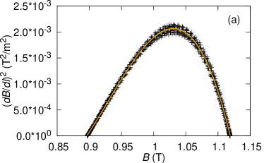
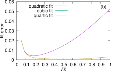
Figure 1: The value of $(dB/d\ell)^{2}$ on the outermost flux surface in the precise QA equilibrium Landreman and Paul (2022) is plotted as a function of $B$, alongside a cubic polynomial fit in (a). In (b), the errors of quadratic, cubic, and quartic fits are compared on each flux surface, demonstrating that a cubic ansatz (as predicted by KdV) is sufficient.

In Fig. 2, we demonstrate that $B$ appears roughly sinusoidal far from the separatrix but becomes soliton-like (sharper peaks, flatter troughs) as the separatrix is approached. Note that the $B$ shown in Fig. 2 is perfectly quasisymmetric, as symmetry-breaking modes have been filtered out. The period of $B$ increases as $L(\psi)\to\infty$ on the separatrix.

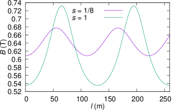
Figure 2: The value of $B$ in a quasiaxisymmetric device in the core ($s=1/8$) and at the edge ($s=1$). The separatrix is outside of the device but close to its edge. Note the increasing period as the separatrix is approached.

With the global description of the exact quasisymmetric $B$, (15) at our disposal, we now investigate a key element of this theory: the physical meaning of the roots $B_{i}$. In Fig. 3 b, we show the typical behavior of the roots. Symmetry-breaking modes have been filtered out, and the roots are obtained by a cubic fit of the numerical data. Points represent the actual minimum and maximum values of $B$ on each flux surface. Surprisingly, the NAE description of $B_{M}$ and $B_{m}$ continues to hold even far from the axis. The third root $B_{X}$ depends quite sensitively on the $\iota$ profiles (Fig. 4). The relationship between the $\iota$ profile, shear, and $B_{X}$ will be studied in more detail in a future publication. For now, we point out that the constant value of $B_{X}$ predicted by the NAE (16) is valid only when the magnetic shear is negligible (see Fig. 3(b)). We show in Fig. 4 that for small but finite shear, $B_{X}$ tracks the $\iota$ profile quite closely but varies more for positive shear.

Understanding the roots enables us to estimate the maximum volume that a quasisymmetric field can occupy since the periodicity of $B$ is maintained as long as $0\leq m<1$. As we saw earlier, the limit $(m\to 1,B_{m}\to B_{X})$ was the limit in which the connection length diverges. Using the simple NAE estimates for the roots $B_{m}$ and $B_{X}$, we can estimate where the two roots will intersect, thereby signaling the breakdown of periodicity. We have demonstrated in Fig. 3 how this estimate can predict the maximum volume of nested surfaces in precise QA extended using coils developed recently. Wechsung et al. (2022) The appearance of the island chain in Fig. 3 is due to the failure of QS (which guarantees nested flux surfaces Rodríguez, Helander, and Bhattacharjee (2020)) and not due to a resonance with the helicity of the QA. Rodríguez and Bhattacharjee (2021)

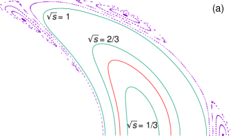
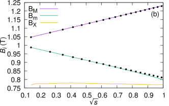
Figure 3: Prediction of maximum toroidal volume that can be made quasisymmetric in precise QA. The boundary of the extended precise QA and two other flux surfaces are shown inside a Poincare plot of the islands in (a), and the roots are plotted in (b). The boundary of the original precise QA is shown in red. Note that the islands occur where the second and third roots touch approximately.

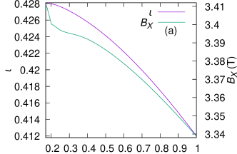
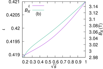
Figure 4: The $B_{X}$ and $\iota$ profiles plotted for precise QA versions with negative shear (a) and positive shear (b).

In summary, we have demonstrated that periodic soliton solutions of the KdV equation lead to a broad class of exactly quasisymmetric $B$. Several results follow from the connection between QS and KdV.

Firstly, the description of a class of exactly quasisymmetric $B$ can be reduced to understanding the behavior of the roots $B_{i}$ of a cubic polynomial. These roots correspond to extrema or saddle points of $B$ on a surface. In particular, $B$, which satisfies the periodic KdV, is a solution of the periodic Schrodinger equation where $B_{i}$’s are related to the endpoints of the band gap.(Kamchatnov, 2000; Novikov et al., 1984) Since the spectrum of KdV is time-independent, the roots do not depend on time. This confirms the well-known statement that the extrema or saddle points of $B$ depend only on the flux label in QS.Helander (2014) Furthermore since various aspects of the flux surface shaping can be deduced (Rodriguez, 2022) from the Fourier coefficients of B, the hidden lower dimensionality is beneficial for understanding shaping.

Secondly, the hierarchy of quasisymmetric invariants, as given by (4), can be understood in terms of the hierarchy of the conserved quantities of KdV. Evolution under KdV guarantees the field-line independence of these quantities. Thirdly, we can estimate the maximum toroidal volume QS allows from the properties of the roots—the overlap of the third root with the second signals the breakdown of periodicity of $B$, as demonstrated numerically. Finally, the connection length can be much larger than the major radius, typically assumed in the literature. A longer connection length may have important implications for linear and nonlinear stability in devices with QS.

Although we have not imposed any constraints from ideal MHD and therefore have avoided the overdetermination problem, we have verified that several existing numerically-obtained configurations are well described by our theory. Given the well-known robust stability of soliton solutions,Tao (2009) further work is needed to elucidate the possible implications for the stability of QS equilibria.

We conclude by thanking E. Rodriguez, H. Weitzner, V. Duarte, F.P. Diaz, and M. Landreman for helpful discussions and suggestions. This research was supported by a grant from the Simons Foundation/SFARI (560651, AB) and DoE Grant No. DE-AC02-09CH11466.

Appendix A Derivation of $\mathcal{D}(\psi)$ in equation (12)

We present here the derivation of the function $\mathcal{D}(\psi)$, which appears in

$$\left(\frac{\partial B}{\partial\ell}\right)^{2}=\mathcal{D}(\psi)(B_{M}-B)(B-B_{m})(B-B_{X}),$$ (12)

in terms of the roots $B_{M}(\psi),B_{m}(\psi),B_{X}(\psi)$, $\iota(\psi)$, the rotational transform, and the quasihelicity $N$. Helander (2014); Landreman and Sengupta (2018)

For the derivation, we shall utilize the following facts. Firstly, $B$ is periodic with period $L(\psi)$. Thus, $B(\ell)=B(\ell+L(\psi))$. Secondly, the average $\oint Bd\ell$ is a flux function. To show this, we use Boozer coordinates $(\psi,\vartheta,\phi)$ Landreman and Sengupta (2018), where the Jacobian is given by

$$\bm{B}\cdot\bm{\nabla}\vartheta=\iota_{N}\frac{B^{2}}{G(\psi)+\iota(\psi)I(\psi)},\quad\iota_{N}=\iota(\psi)-N.$$ (17)

Note that $G(\psi),I(\psi)$ are flux functions related to the poloidal and toroidal currents. Helander (2014) Since $\bm{B}\cdot\bm{\nabla}=B\partial_{\ell}$ in $(\psi,\alpha,\ell)$, (17) takes the form

$$\frac{\partial\theta}{\partial\ell}=\iota_{N}\frac{B}{G+\iota I}.$$ (18)

Integrating (18) with respect to $\ell$ from $0$ to $L$ and noting that the net change in the Boozer angle $\theta$ is $2\pi$, we get

$$\int_{0}^{L}Bd\ell=2\pi\frac{G+\iota I}{\iota_{N}}.$$ (19)

Finally, we shall need some basic identities satisfied by elliptic functions (see Appendix A of reference [28]). In particular, we shall use

$$\text{dn}(z,m)=\text{dn}(z+2\text{K}(m),m)$$

$$\text{dn}^{2}(z,m)=1-m+m\text{cn}^{2}(z,m)$$

$$\int_{0}^{\text{K}(m)}\text{dn}^{2}(u,m)du=\text{E}(m),$$ (20)

where dn$(z,m)$, cn$(z,m)$ are standard Jacobi elliptic functions, and K$(m)$, E$(m)$ are the complete elliptic integrals of the first and second kind.Kamchatnov (2000)

We are now in a position to derive an expression for $\mathcal{D}(\psi)$. To simplify the derivation, we shall work in the frame of reference where $\partial_{\alpha}B=0$ (see discussion under (3)). In this frame, the solution to (12) is

$$B =B_{X}+(B_{M}-B_{X})\text{dn}^{2}\left(\sqrt{\frac{B_{M}-B_{X}}{2}}\sqrt{\frac{\mathcal{D}}{2}}\ell,m\right),$$

$$m =\frac{B_{M}-B_{m}}{B_{M}-B_{X}},\quad 0\leq m\leq 1,$$ (21)

which follows from (13),(15) and (20).

From the periodicity of $B$ and the Jacobi elliptic function dn (20), it follows that

$$\sqrt{\mathcal{D}}L(\psi)=\frac{4\text{K}(m)}{\sqrt{B_{M}-B_{X}}}.$$ (22)

Moreover, integrating (21) over $\ell$ we obtain

$$\int_{0}^{L}Bd\ell=L\left(B_{X}+(B_{M}-B_{X})\frac{\text{E}(m)}{\text{K}(m)}\right)$$ (23)

Combining together the two different expressions of the $\oint Bd\ell$ given by (19) and (23), and using the relation between $\mathcal{D}$ and $L$ from (22), we finally obtain

$$\sqrt{\mathcal{D}}=\frac{\iota_{N}}{G+\iota I}\frac{\text{K}(m)}{\pi/2}\frac{\left(B_{X}+(B_{M}-B_{X})\frac{\text{E}(m)}{\text{K}(m)}\right)}{\sqrt{B_{M}-B_{X}}}$$ (24)

Appendix B Additional configurations that satisfy the integrated KdV equation (12)

Here, we present figures similar to Figs. 1 and 3 in the main text, using data from different stellarator devices.

The precise QA configuration with larger negative shear in Fig. 6 was obtained by a series of optimizations starting from the precise QA.Landreman and Paul (2022) Specifically, we start from the same objective function used to optimize the precise QA, and the precise QA configuration itself. The mean shear $\bar{\hat{s}}$ was extracted from the precise QA configuration, and a new least-squares term $(\bar{\hat{s}}-\bar{\hat{s}}_{*})^{2}$ was added to the objective function, where the target value for mean shear $\bar{\hat{s}}_{*}$ is taken to be slightly different from the extracted value. This new objective is then optimized locally, using the precise QA as the initial state. This ensures that the additional least-squares term is almost zero, so the precise QA is approximately an optimum to the modified objective function. Hence, the new local optimum can be expected to be close to the initial configuration. This process is then repeated starting from the slightly modified optimum, each step generating a similar equilibrium with a slightly different mean shear. Mean shear is here defined as $b/\bar{\iota}$, where $b$ is the result of fitting a first-order polynomial $a+bs$ to the iota profile, where $s$ is the normalized toroidal flux; $\bar{\iota}$ is the rotational transform averaged over all radii. The mean shear in the original precise QA is about $-0.018$, and we incremented the target negative shear in steps of $0.005$.

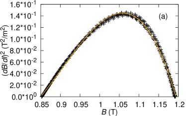
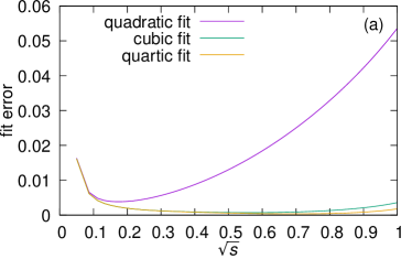
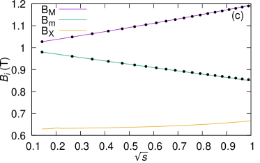
Figure 5: The value of $(dB/d\ell)^{2}$ on the outermost flux surface in the precise QH Landreman and Paul (2022) as a function of $B$, alongside a cubic polynomial fit (a), and the errors of quadratic, cubic, and quartic fits on each flux surface (b). Panel (c) shows the behavior of the roots in the precise QH.

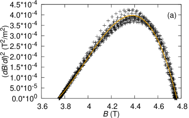
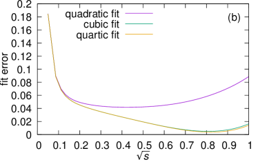
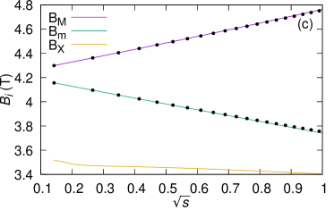
Figure 6: The value of $(dB/d\ell)^{2}$ on the outermost flux surface in a precise QA version with average shear -0.08 as a function of $B$, alongside a cubic polynomial fit (a), and the errors of quadratic, cubic, and quartic fits on each flux surface (b). Panel (c) shows the behavior of the roots in this version of the precise QA.

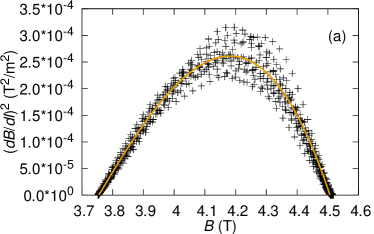
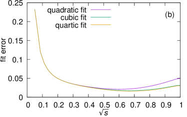
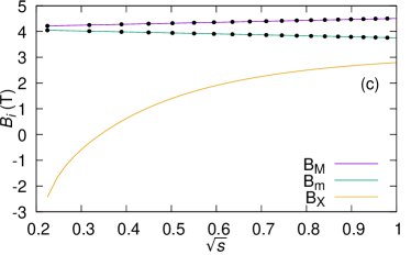
Figure 7: The value of $(dB/d\ell)^{2}$ on the outermost flux surface in a precise QA version with average shear 0.04 as a function of $B$, alongside a cubic polynomial fit (a), and the errors of quadratic, cubic, and quartic fits on each flux surface (b). Panel (c) shows the behavior of the roots in this version of the precise QA.

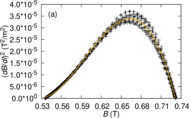
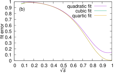
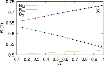
Figure 8: The value of $(dB/d\ell)^{2}$ on the outermost flux surface in the QA equilibrium that was used in Figure 2 in the main text as a function of $B$, alongside a cubic polynomial fit (a), and the errors of quadratic, cubic, and quartic fits on each flux surface (b). Panel (c) shows the behavior of the roots in this QA equilibrium.

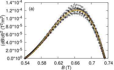
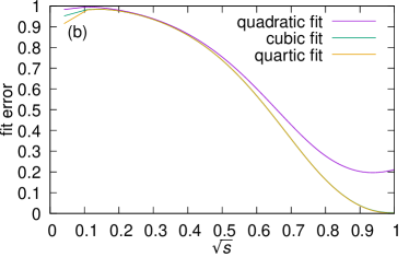
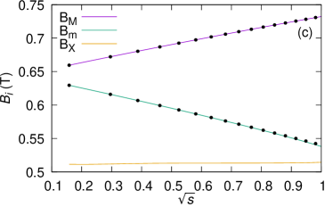
Figure 9: The value of $(dB/d\ell)^{2}$ on the outermost flux surface in a QA equilibrium similar to that in Fig. 8 as a function of $B$, alongside a cubic polynomial fit (a), and the errors of quadratic, cubic, and quartic fits on each flux surface (b). Panel (c) shows the behavior of the roots in this QA equilibrium.

Figs. 8 and 9 show equilibria that were not derived from the precise QA/QH. Instead, they were only optimized for quasisymmetry on the outermost flux surface, with the quasisymmetry degrading as the axis is approached. For both cases, the ratio of symmetry-breaking modes to quasisymmetric modes near the axis is $\sim 10^{-3}$. While this may seem a small value, the resulting ripple creates enough noise in the $(dB/d\ell)^{2}$ vs. $B$ plot to render it meaningless, and the error for all fits is $\sim 1$ in that region. The symmetry-breaking modes were filtered out when calculating the roots shown in panels (c). Note that the equilibrium shown in Fig. 8 is the same one used in Fig. 2 in the main text.

References

- Charalambous, Dubovsky, and Ivanov (2021) P. Charalambous, S. Dubovsky, and M. M. Ivanov, “Hidden symmetry of vanishing love numbers,” Physical Review Letters 127, 101101 (2021).
- Lee et al. (2021) D. Lee, S. Bogner, B. A. Brown, S. Elhatisari, E. Epelbaum, H. Hergert, M. Hjorth-Jensen, H. Krebs, N. Li, B.-N. Lu, et al., “Hidden spin-isospin exchange symmetry,” Physical Review Letters 127, 062501 (2021).
- Liu and Tegmark (2022) Z. Liu and M. Tegmark, “Machine learning hidden symmetries,” Physical Review Letters 128, 180201 (2022).
- Landreman and Paul (2022) M. Landreman and E. Paul, “Magnetic fields with precise quasisymmetry for plasma confinement,” Physical Review Letters 128, 035001 (2022).
- Moser (1979) J. Moser, “Hidden symmetries in dynamical systems,” American Scientist 67, 689–695 (1979).
- Leach and Andriopoulos (2008) P. G. Leach and K. Andriopoulos, “The ermakov equation: a commentary,” Applicable Analysis and Discrete Mathematics , 146–157 (2008).
- Ovsienko and Khesin (1987) V. Y. Ovsienko and B. A. Khesin, “Korteweg-de vries superequation as an euler equation,” Functional Analysis and Its Applications 21, 329–331 (1987).
- Gardner et al. (1967) C. S. Gardner, J. M. Greene, M. D. Kruskal, and R. M. Miura, “Method for solving the korteweg-devries equation,” Physical review letters 19, 1095 (1967).
- Novikov et al. (1984) S. Novikov, S. V. Manakov, L. P. Pitaevskii, and V. E. Zakharov, Theory of solitons: the inverse scattering method (Springer Science & Business Media, 1984).
- Lewis Jr (1967) H. R. Lewis Jr, “Classical and quantum systems with time-dependent harmonic-oscillator-type hamiltonians,” Physical Review Letters 18, 510 (1967).
- Gjaja and Bhattacharjee (1992) I. Gjaja and A. Bhattacharjee, “Asymptotics of reflectionless potentials,” Physical review letters 68, 2413 (1992).
- Brezhnev (2008) Y. V. Brezhnev, “What does integrability of finite-gap or soliton potentials mean?” Philosophical Transactions of the Royal Society A: Mathematical, Physical and Engineering Sciences 366, 923–945 (2008).
- Berry and Howls (1990) M. Berry and C. Howls, “Fake airy functions and the asymptotics of reflectionlessness,” Journal of Physics A: Mathematical and General 23, L243 (1990).
- Boozer (1983) A. H. Boozer, “Transport and isomorphic equilibria,” The Physics of Fluids 26, 496–499 (1983).
- Helander (2014) P. Helander, “Theory of plasma confinement in non-axisymmetric magnetic fields,” Reports on Progress in Physics 77, 087001 (2014).
- Rodriguez (2022) E. Rodriguez, “Quasisymmetry,” Ph.D. thesis (2022).
- Freidberg (2014) J. P. Freidberg, Ideal MHD (Cambridge University Press, 2014) p. 302.
- Burby, Kallinikos, and MacKay (2020) J. W. Burby, N. Kallinikos, and R. S. MacKay, “Some mathematics for quasi-symmetry,” Journal of Mathematical Physics 61, 093503 (2020).
- Plunk and Helander (2018) G. G. Plunk and P. Helander, “Quasi-axisymmetric magnetic fields: weakly non-axisymmetric case in a vacuum,” Journal of Plasma Physics 84, 905840205 (2018).
- Garren and Boozer (1991a) D. A. Garren and A. H. Boozer, “Magnetic field strength of toroidal plasma equilibria,” Physics of Fluids B: Plasma Physics 3, 2805–2821 (1991a).
- Garren and Boozer (1991b) D. A. Garren and A. H. Boozer, “Existence of quasihelically symmetric stellarators,” Physics of Fluids B: Plasma Physics 3, 2822–2834 (1991b).
- Landreman and Sengupta (2019) M. Landreman and W. Sengupta, “Constructing stellarators with quasisymmetry to high order,” Journal of Plasma Physics 85, 815850601 (2019).
- Constantin, Drivas, and Ginsberg (2021) P. Constantin, T. D. Drivas, and D. Ginsberg, “On quasisymmetric plasma equilibria sustained by small force,” Journal of Plasma Physics 87, 905870111 (2021).
- Rodríguez, Helander, and Bhattacharjee (2020) E. Rodríguez, P. Helander, and A. Bhattacharjee, “Necessary and sufficient conditions for quasisymmetry,” Physics of Plasmas 27, 062501 (2020).
- Rodríguez, Sengupta, and Bhattacharjee (2022) E. Rodríguez, W. Sengupta, and A. Bhattacharjee, “Weakly quasisymmetric near-axis solutions to all orders,” Physics of Plasmas 29, 012507 (2022).
- Landreman and Sengupta (2018) M. Landreman and W. Sengupta, “Direct construction of optimized stellarator shapes. Part 1. Theory in cylindrical coordinates,” Journal of Plasma Physics 84, 905840616 (2018).
- Schief (2003) W. Schief, “Nested toroidal flux surfaces in magnetohydrostatics. generation via soliton theory,” Journal of plasma physics 69, 465–484 (2003).
- Kamchatnov (2000) A. M. Kamchatnov, Nonlinear periodic waves and their modulations: an introductory course (World Scientific, 2000).
- Courant and Snyder (1958) E. D. Courant and H. S. Snyder, “Theory of the alternating-gradient synchrotron,” Annals of physics 3, 1–48 (1958).
- Magnus and Winkler (2013) W. Magnus and S. Winkler, Hill’s equation (Courier Corporation, 2013).
- Lax (1968) P. D. Lax, “Integrals of nonlinear equations of evolution and solitary waves,” Communications on pure and applied mathematics 21, 467–490 (1968).
- Tao (2009) T. Tao, “Why are solitons stable?” Bulletin of the American Mathematical Society 46, 1–33 (2009).
- Gesztesy and Weikard (1996) F. Gesztesy and R. Weikard, “Picard potentials and hill’s equation on a torus,” Acta Mathematica 176, 73–107 (1996).
- Dubrovin, Krichever, and Novikov (1990) B. A. Dubrovin, I. M. Krichever, and S. P. Novikov, “Integrable systems. i,” in Dynamical systems IV (Springer, 1990) pp. 173–280.
- Froman (1979) N. Froman, “Dispersion relation for energy bands and energy gaps derived by the use of a phase-integral method, with an application to the Mathieu equation,” Journal of Physics A: Mathematical and General 12, 2355 (1979).
- Wechsung et al. (2022) F. Wechsung, M. Landreman, A. Giuliani, A. Cerfon, and G. Stadler, “Precise stellarator quasi-symmetry can be achieved with electromagnetic coils,” Proceedings of the National Academy of Sciences 119, e2202084119 (2022).
- Rodríguez and Bhattacharjee (2021) E. Rodríguez and A. Bhattacharjee, “Islands and current singularities in quasisymmetric toroidal plasmas,” Physics of Plasmas 28, 092506 (2021).