De Haas-van Alphen effect and quantum oscillations as a function of temperature in correlated insulators

Abstract

We propose and study a theoretical model of insulators which show de Haas-van Alphen oscillations as well as periodic dependence of the magnetization on inverse temperature. The insulating behavior is due to the Coulomb interaction driven hybridization of fermions at the crossing point of their energy bands. We show that the leading contribution to the oscillations at small magnetic fields is due to the oscillatory dependence of the hybridization gap on the magnetic field. In order to see this the hybridization is derived from a self-consistent non-linear equation. We show that the amplitude of the de Haas-van Alphen is periodic in inverse temperature with a period defined by a combination of the hybridization gap and magnetic field. Moreover, we predicted that the amplitude must vanish at a particular field proportional to the hybridization gap.

We are motivated by recent experiments where quantum oscillations in Kondo insulator SmB₆ were observed LiScience2014 ; SuchitraScience2015 ; SuchitraNatPhys2017 ; SuchitraScience2020 . This material becomes insulating below about $T_{\mathrm{c}}=40\mathrm{K}$ due to the gapping of the Fermi surface. Observed quantum oscillations occur only in the magnetization, i.e. de Haas - van Alphen (dHvA) effect, while electric resistivity doesn’t show any oscillations (absence of Shubnikov - de Haas effect). The latter is due to after all insulating behavior, while occurance of dHvA oscillations in insulators poses a mystery. Not to mention that the observed frequency of dHvA oscillations of the insulator is that of the metallic phase of the system, before it turned insulating via a gapping mechanism. In addition, the frequency is similar to the one of the LaB₆ metallic material, which never turns insulating and which has a similar band structure with the metallic phase of the SmB₆.

There are theories which propose emergence of neutral quasiparticles with Fermi surface that somehow nevertheless couple to the magnetic field to show dHvA effect but not the electric field, or of fermions that fractionalize to either Majoranas or other exotic structures BaskaranArxiv ; SodemannChowdhurySenthil ; VarmaPRB . Whether these theories can explain the experiments LiScience2014 ; SuchitraScience2015 ; SuchitraNatPhys2017 ; SuchitraScience2020 is currently under debate. There are theories which obtain dHvA quantum oscillations in insulators based on the non-interacting fermions KnolleCooperPRL15 ; PalArxiv2022 . SmB₆ insulator is known to be strongly correlated (see for example Hewson ), and it is rather odd to expect that the non-interacting picture will fully explain its physical properties.

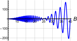
Figure 1: Plot of the first harmonic of the oscillating part of the torque, i.e. of $M_{osc}B$ where $M_{\mathrm{osc}}$ is given by Eq. (1) for $2\theta_{0}\approx 40K$, effective mass is picked to be $m=0.2m_{\mathrm{e}}$, at $T=0$, and $\mu m/m_{\mathrm{e}}=420T$.

In our theory the two fermions hybridize with each other via the repulsive Coulomb interaction. As a result, a gap opens up at their energy band crossing points resulting in an insulator when the Fermi level is at the crossing point. Free energy gets minimized as a result of the hybridization. The magnetic field quantizes the energy spectrum of fermions forming Landau levels. Then an intuitive picture of the effect of quantium oscillations in insulators is that when the Landau levels of two fermion branches cross each other, the hybridization is maximised, while when the Landau levels distance apart, the hybridization is minimized. To see this effect analytically, the hybridization must be treated self-consistently and obtained from the non-linear equation. Finally, since the free energy gain is proportional to the second power of the hybridization, the magnetization and specific heat are expected to be oscillating functions of the magnetic field. It turns out that the frequency of oscillations equals to the energy of the energy bands crossing point, and is related to the Fermi energy of the metallic phase before the hybridization (this fact was known since KnolleCooperPRL15 ). The response of the system due to the described mechanism is found to be diamagnetic (Landau diamagnetism) and the non-oscillating part of the magnetization is proportional to the magnetic field $B$. The oscillating part of the magnetization $M$ at small magnetic fields and at zero temperature can be best described with

$$M_{\mathrm{osc}}=\frac{2\mu}{\pi\theta_{0}}\left(\frac{2\pi\theta_{0}}{B}\right)^{\frac{3}{2}}\left(1-\frac{B}{2\pi\theta_{0}}\right)\sin\left(\frac{2\pi\mu}{B}-\pi\right)e^{-4\pi\frac{\theta_{0}}{B}},$$ (1)

where $\mu$ is the Fermi energy of the metallic phase and $2\theta_{0}$ is the non-oscillating part of the hybridization gap, and where we keep $B$ in units of cyclotron frequency. Smallness of the magnetic field is given by the $8\pi\theta_{0}>B$ condition, which falls in in to the experimental regime. Despite of the exponential suppression, in reality of the experiments in which $2\theta_{0}\approx 40K$ with the effective mass picked to be $m=0.2m_{\mathrm{e}}$ (where $m_{\mathrm{e}}$ is bare electron’s mass), Eq. (1) gives sizable contribution at small magnetic fields. We plot oscillating part of the torque in Fig. (1). Having presented our main results for zero temperature, in the rest of the paper we outline analytical arguments which lead to them and expand the list of our results to the non-zero temperature. Each step of the calculations is outlined in details in the Supplemental Material (SM) SM .

We consider a model Hamiltonian keeping in mind a SmB₆ system.

$$H_{0}=\int_{\bf k}\bar{\psi}\left[\begin{array}[]{cc}\xi_{\bf k}&0\\ 0&\epsilon_{0}\end{array}\right]\psi\equiv\int_{\bf k}\bar{\psi}h\psi,$$ (4)

where $\xi_{\bf k}=\frac{{\bf k}^{2}}{2m}-\mu$, notation $\int_{\bf k}(..)=\int\frac{d{\bf k}}{(2\pi)^{2}}(..)$ was used, then $\epsilon_{0}=E_{0}-\mu=\mathrm{const}$, which we will set $\epsilon_{0}=0$ without losing generality, where $\mu$ is the chemical potential, and $\bar{\psi}=\left[\bar{\phi}_{\mathrm{d}},~{}\bar{\phi}_{\mathrm{f}}\right],$ and the same for $\psi$. In order to present analytic arguments we assume that the system is two-dimensional. Three-dimensional case is slightly more analytically involved, but will also be described by the presented below arguments. We consider spinless fermions for simplicity, and note that all of the results below will not change if the $f-$ fermion’s spectrum had a dispersion. Interaction between the two types of fermions is

$$H_{\mathrm{int}}=U\int_{x}\bar{\phi}_{\mathrm{d}}(x)\phi_{\mathrm{d}}(x)\bar{\phi}_{\mathrm{f}}(x)\phi_{\mathrm{f}}(x),$$ (5)

where $U>0$ corresponds to repulsion. We decouple interaction Eq. (5) using the Hubbard-Stratonovich transformation, and keeping in mind the transformation is made with the action, we write the result, $-\left(\bar{\theta}+\bar{\phi}_{\mathrm{d}}\phi_{\mathrm{f}}U\right)U^{-1}\left(\theta+U\bar{\phi}_{\mathrm{f}}\phi_{\mathrm{d}}\right)+U\bar{\phi}_{\mathrm{d}}\phi_{\mathrm{f}}\bar{\phi}_{\mathrm{f}}\phi_{\mathrm{d}}=-\bar{\theta}U^{-1}\theta-\bar{\phi}_{\mathrm{d}}\phi_{\mathrm{f}}\theta-\bar{\theta}\bar{\phi}_{\mathrm{f}}\phi_{\mathrm{d}}.$ Bilinear in fermion fields term introduces hybridization between $d-$ and $f-$ fermions, described by the Hamiltonian

$$H_{\mathrm{int};1}=\int_{\bf k}\bar{\psi}\left[\begin{array}[]{cc}0&\theta\\ \bar{\theta}&0\end{array}\right]\psi\equiv\int_{\bf k}\bar{\psi}h_{\mathrm{int};1}\psi.$$ (8)

Assuming that $\theta$ and $\bar{\theta}$ are constants in space (mean field approximation), the spectrum of fermions described by Hamiltonian $h+h_{\mathrm{int};1}$ becomes

$$\epsilon_{{\bf k},\pm}=\frac{\xi_{\bf k}+\epsilon_{0}}{2}\pm\sqrt{\left(\frac{\xi_{\bf k}-\epsilon_{0}}{2}\right)^{2}+\bar{\theta}\theta},$$ (9)

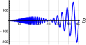
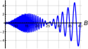
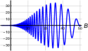
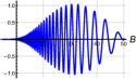
Figure 2: Left: plot of the first harmonic of the oscillating part of the torque, i.e. of $M_{osc}B$ where $M_{\mathrm{osc}}$ is given by Eq. (117) for $2\theta_{0}\approx 40T$. Top: effective mass is $m=0.2m_{\mathrm{e}}$; Bottom: $m=0.4m_{\mathrm{e}}$. Right: magnetization for the same parameters. All plots are for $T=0$ and $\mu m/m_{\mathrm{e}}=420T$.

which are schematically plotted in Fig. (2). There is a gap opening at the cross-section of the energy bands of $d-$ and $f-$ fermions due to the hybridization.

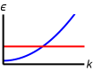
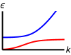
Figure 2: Spectrum of fermions before (left) and after (right) the hybridization. The hybridization gap $2\theta$ opens at the crossing point.

Next, we need to find the structure of the hybridization. For that, as usual, we integrate our fermions and minimize the action with respect to the hybridization, and get self-consistent equation for the hybridization,

$$\theta=U\theta\int_{\bf k}\frac{{\cal F}_{\epsilon_{{\bf k},+}}-{\cal F}_{\epsilon_{{\bf k},-}}}{\epsilon_{{\bf k},+}-\epsilon_{{\bf k},-}},$$ (10)

where ${\cal F}_{\epsilon}=\tanh\left(\frac{\epsilon}{2T}\right)$ is the Fermi-Dirac distribution function where $T$ is the temperature.

A magnetic field perpendicular to the plane of the system is added. It results in the Landau quantization of the energy spectrum, such that $\xi_{\bf k}\rightarrow\xi_{n}=B(n+\frac{1}{2})-\mu$, where $n>0$ is an integer denoting corresponding Landau level. We note that here and everywhere below we count $B$ in terms of cyclotron energy $\omega_{B}=\frac{eB}{mc}$, where $m$ is the mass of $d-$ fermions. With that we rewrite Eq. (10) for the system in the applied magnetic field,

$$1=UB\sum_{n}\frac{{\cal F}_{\epsilon_{n,+}}-{\cal F}_{\epsilon_{n,-}}}{\sqrt{(Bn+\frac{B}{2}-\mu)^{2}+4\bar{\theta}\theta}},$$ (11)

where now summation is over the Landau levels. To sum over the Landau levels, we utilize Poisson summation formula

$$\sum_{n=0}g(n)=\int_{0}^{\infty}g(x)dx+\sum_{p\neq 0}\int_{0}^{\infty}e^{i2\pi px}g(x)dx,$$ (12)

where $g(n)$ is some function. We will first obtain all of the results for $T=0$. With that when the Fermi energy is in the gap, the upper band is deoccupied meaning ${\cal F}_{\epsilon_{n,+}}=1$, and the lower band is completely filled, ${\cal F}_{\epsilon_{n,-}}=-1$. As a result, the non-linear equation is solved with

$$\theta=\theta_{0}+2\theta_{0}\cos\left(2\pi\frac{\mu}{B}-\pi\right)e^{-\frac{4\pi\theta_{0}}{B}}\sqrt{\frac{B}{2\pi\theta_{0}}},$$ (13)

in the limit $8\pi\frac{\theta_{0}}{B}>1$, which allowed us to pick only $p=\pm 1$ in the Poisson summation formula because harmonics with $n>1$ decay with a $e^{-\frac{4\pi\theta_{0}}{B}n}$ factor. Here $\theta_{0}=\sqrt{\mu^{2}-\frac{B^{2}}{4}}e^{-\frac{1}{4U}}$ is the non-oscillating part of the solution. The free energy of the hybridized system reads $F=-\theta^{2}+F_{\Sigma}$, where $F_{\Sigma}$ is the part of the free energy corresponding to the oscillation in magnetic field of the non-interacting system, i.e. to the system with constant hybridization $\theta_{0}$. We note that it is not $-\frac{\theta^{2}}{2U}$ that enters the free energy as it gets cancelled troughout the derivation, but just like in the BCS theory it is rather $-\theta^{2}$. Collecting oscillation terms from both parts of free energy, i.e. from $-\theta^{2}$ and $F_{\Sigma}$, we get

$$\delta F_{\mathrm{osc}} =-4\theta_{0}^{2}\sqrt{\frac{B}{2\pi\theta_{0}}}\left(1-\frac{B}{2\pi\theta_{0}}\right)$$

$$\times\cos\left(\frac{2\pi\mu}{B}-\pi\right)e^{-\frac{4\pi\theta_{0}}{B}},$$ (14)

here $1$ in the round brackets is the first main result of the present paper, it originated from the oscillations of the hybridization and is due to the interactions. The term $-\frac{B}{2\pi\theta_{0}}$ in the round brackets is non-interacting, came from oscillating part of $F_{\Sigma}$ and corresponds to the results of Refs. KnolleCooperPRL15 ; PalArxiv2022 . Essentially, it corresonds to the oscillations in magnetic field of the fully filled fermion band $\epsilon_{{\bf k};-}$. It is clear that the latter term is smaller than the former at small magnetic fields defined by the $2\pi\frac{\theta_{0}}{B}>1$ condition. When $\frac{B}{2\pi\theta_{0}}=1$ the amplitude vanishes, and at larger fields the non-interacting part will become dominant. We note that vanishing AokiJPSJ2014 and a decrease Li_PRX2022 of the amplitude was observed in strongly correlated systems AokiJPSJ2014 ; Li_PRX2022 and attributed to the field driven metamagnetic transition. Proposed here mechanism might be relevant to the experiments AokiJPSJ2014 ; Li_PRX2022 , but more details are needed. We differentiate the oscillating part of minus the free energy Eq. (De Haas-van Alphen effect and quantum oscillations as a function of temperature in correlated insulators) with respect to the magnetic field and obtain Eq. (1) by keeping only the term $\propto\mu$.

We observe that the response of the system due to the hybridization mechanism is diamagnetic. This is precisely due to the magnetic field dependence of the non-oscillating part of the hybrdidization $\theta_{0}$ defined after Eq. (13). Indeed, the non-oscillating part of the magnetization is $M\propto-\partial_{B}(-\theta_{0}^{2})=-\frac{B}{2}e^{-\frac{1}{2U}}$. Physics of obtained diamagnetism is that the system wants to expel the magnetic field in order to minimize the energy associated with the Coulomb repulsion. Another point is that the calculations suggest that we could have had any quadratic in magnetic field structure under the square root in the definition of $\theta_{0}$, for example $\sqrt{\mu^{2}-\frac{B^{2}}{4}+aB}$, where $a$ is some energy, then there would be spontaneous magnetic order in the system characterized by a finite magnetization. This is experimentally not the case LiScience2014 , hence the choice of $a=0$. Moreover, we wish to point out that $-\frac{B^{2}}{4}$ in $\theta_{0}=\sqrt{\mu^{2}-\frac{B^{2}}{4}}e^{-\frac{1}{4U}}$ is due to the lowest Landau level.

Let us now discuss temperature dependence of the amplitude of the dHvA oscillations. The non-linear equation at finite temperature is given in Eq. (10), where the temperature is in the Fermi-Dirac distribution functions. With all the technical steps presented in the SM SM to the paper, we here breifly outline the steps. Eq. (10) is modified to the presence of the magnetic field, summation over the Landau levels is performed again with the help of the Poisson summation formula Eq. (12). The non-oscillating in magnetic field terms are barely changed at finite temperatures. However, the terms which result in dHvA effect are drastically modified by the non-zero temperature. The distribution functions introduce residues, and it turns out it is convenient to integrate over the Poisson variable by introducing a contour which embraces certain residues which ensure convergence, such that the integral over the Poisson variable is reduced to the sum over the residues. Then the sum over the residues is calculated by using the Poisson summation formula Eq. (12) for the second time. As a result of the summation an oscillation with the inverse temperature of the hybrdization appears. Then the obtained solution for the hybridization Eq. (13) at zero temperature gets updated in accord with the mentioned steps as

$$\theta=\theta_{0}(T)+2\theta_{0}(T)\cos\left(2\pi\frac{\mu}{B}-\pi\right)R(T),$$ (15)

where $R(T)=\sum_{n=-\infty}^{+\infty}R_{n}(T)$ is a result of the Poisson summation formula with elements

$$R_{n}(T)=\int_{0}^{+\infty}\frac{e^{i2\pi nx}}{x+\frac{1}{2}}e^{-\frac{2\pi\theta_{0}}{B}\left[\frac{1}{2\pi\frac{T}{\theta_{0}}\left(x+\frac{1}{2}\right)}+2\pi\frac{T}{\theta_{0}}\left(x+\frac{1}{2}\right)\right]}dx,$$ (16)

where $x+\frac{1}{2}$ is reminiscent of the Matsubara frequency. We plot $R_{0}(T)$ in Fig. 3 to suggest that except for the shoulder it is consistent with standard Lishits-Kosevich formula.

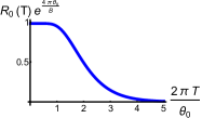
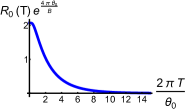
Figure 3: Plot of the numerically estimated expression Eq. (16) for $n=0$ times the $e^{\frac{4\pi\theta_{0}}{B}}$ factor for left $\frac{2\theta_{0}}{B}=1$ and right for $\frac{2\theta_{0}}{B}=0.2$. It is approximately consistent with standard Lifshits-Kosevich structure.

It is now instructive to perform the steepest descent approximation in evaluating the $R_{0}(T)$, we get the following limiting expressions $R_{0}(T=0)=e^{-\frac{4\pi\theta_{0}}{B}}\sqrt{\frac{B}{2\theta_{0}}},$ and $R_{0}(T\rightarrow\infty)\approx\frac{B}{4\pi^{2}T}e^{-\frac{4\pi\theta_{0}}{B}}e^{-\pi\frac{\theta_{0}}{2H}\left(\frac{2\pi T}{\theta_{0}}\right)^{2}}.$ Indeed, the $T=0$ limit is consistent with the Eq. (13), and the $T\rightarrow\infty$ decay is consistent with the Lishits-Kosevich expression.

Having understood $R_{0}(T)$ let us now add higher harmonics. We work in the regime when the solution for the gap Eq. (15) is valid. We plot $R(T)$ as a function of temperature in Figs. (4) and (5). to describe shown dependence we can approximate the integral with the steepest descent method and obtain in the vicinity of the peak,

$$R(T)\approx R_{0}(T)\left[1+2\sum_{n=1}\cos\left(\frac{\theta_{0}}{T}\bar{z}n-\pi n\right)e^{-\frac{2\pi^{2}n^{2}}{|g(\bar{z})|}}\right],$$ (17)

where saddle-point is at

$$\bar{z}=\frac{4\pi\theta_{0}}{B+\sqrt{B^{2}+(4\pi\theta_{0})^{2}}},$$ (18)

and $g(\bar{z})=\left(\frac{2\pi T}{\theta_{0}}\right)^{2}\frac{1}{\bar{z}^{3}}\left(\bar{z}-\frac{4\pi\theta_{0}}{B}\right)$, and a first maximum in the temperature dependence of Eq. (17) occurs at $\frac{\theta_{0}}{T_{\mathrm{peak}}}\bar{z}=\pi$ which reads

$$T_{\mathrm{peak}}=\frac{4\theta_{0}^{2}}{{B+\sqrt{B^{2}+\left(4\pi\theta_{0}\right)^{2}}}}.$$ (19)

Let us first discuss the case of relatively small magnetic fields, $4\pi\theta_{0}>B$. In particular, in Fig. (4) we plot $R(T)$ for $2\theta_{0}=B$. The position of the peak defined in Eq. (19) can be approximated to be

$$T_{\mathrm{peak}}=\frac{\theta_{0}}{\pi}.$$ (20)

To justife our approximation, we plot $\propto\cos\left(\frac{\theta_{0}}{T}\right)$ together with $R(T)$ in Fig. (4). The approximation Eq. (17) works well in the vicinity of the peak, away from it one has to include more terms to make sure the function is positive-definite. As a proof of principle, when the parameter $\frac{2\theta_{0}}{B}$ increases, the amplitude of Eq. (17) exponentially decreases due to the decaying $e^{-4\pi\frac{\theta_{0}}{B}}$ term, however, with that more oscillation cycles appear. For example, see Fig. (5) for the plot for $\frac{2\theta_{0}}{B}=3$, where the position of the peak is consistent with analytical predictions Eq. (20). In addition, we analytically found that $R(T_{\mathrm{peak}})\approx 2e^{-\frac{4\pi\theta_{0}}{B}}$, which is indeed plotted in Fig. (4) and in the left plot in Fig. (5). Non-zero temperature expression for the magnetization reads as

$$M_{\mathrm{osc}}= \frac{2\mu}{\pi\theta_{0}}\left(\frac{2\pi\theta_{0}}{B}\right)^{\frac{5}{2}}R(T)\left(1-\frac{B}{2\pi\theta_{0}}\right)\sin\left(\frac{2\pi\mu}{B}-\pi\right),$$ (21)

where $R(T)$ is given by primarily Eq. (16), and with Eqs. (17) approximating the behavior in the vicinity of the peak.

Let us now discuss relatively large magnetic fields $B\sim 4\pi\theta_{0}$ and $B>4\pi\theta_{0}$. We plot $R(T)$ in Fig. (5) right for $\frac{2\theta_{0}}{B}=0.2$. Unfortunately, the steepest descent method fails to work well in this regime. We, nevertheless, still can predict the existence of the peak in the amplitude due to the oscillations. From the right plot of Fig. (5) we observe that for $\frac{2\theta_{0}}{B}=0.2$ the position of the peak is at $\frac{2\pi T^{(\mathrm{plot})}_{\mathrm{peak}}}{\theta_{0}}\approx 1.32$ which should be compared with the corresponding quantity from the Eq. (19), which is $\frac{2\pi T^{(\mathrm{analytics})}_{\mathrm{peak}}}{\theta_{0}}\approx 0.96$. It turns out that for whatever reason a better approximation is $T^{*}_{\mathrm{peak}}=\frac{2\theta_{0}^{2}}{B}$ which is a high field limit of Fig. (5) and which gives $\frac{2\pi T^{*}_{\mathrm{peak}}}{\theta_{0}}\approx 1.25$. A peak in the amplitude of the dHvA oscillations was experimentally observed at small temperatures in SuchitraScience2015 ; SuchitraNatPhys2017 ; SuchitraScience2020 . In paricular of interest is Fig. 7c in SuchitraScience2020 , where a mismatch of Lifshits-Kosevich formula with the observed temperature dependence of the amplitude was observed. We think that the peak structure in $R(T)$ plotted in the right figure of Fig. (5) might explain the mismatch.

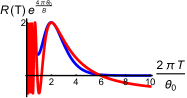
Figure 4: Left: plot of the expression $R(T)$ for $\frac{2\theta_{0}}{B}=1$. Right: the same but with $\left[1-2\cos\left(\frac{\theta_{0}}{T}\right)\right]\frac{2}{3}$ in red plotted together.

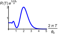
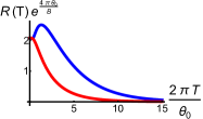
Figure 5: Left: plot of the expression for $R(T)e^{\frac{4\pi\theta_{0}}{B}}$ for $\frac{2\theta_{0}}{B}=3$, which makes it $R(T)e^{6\pi}$, as a proof of principle. The magnitude is exponentially suppressed but with that more oscillation cycles, as compared with the first one if going from large temperatures, become visible. Position of the first peak is consistent with analytical predictions Eq. (20). Right: in blue is the plot of $R(T)$ which has a peak structure, and in red we repeat right plot of Fig. (3), both for $\frac{2\theta_{0}}{B}=0.2$.

In addition to the discussed above, we find a new regime of oscillations occuring in rather strong magnetic fields, $B>8\pi\theta_{0}$. There in the course of the oscillations the hybridization gap vanishes at the minimum of the cycle and then emerges back at the peak. We speculate that such an oscillation can undergo with a phase separation to metallic and insulating domains. Unfortunately, it can’t be experimentally found in the SmB₆ material due to the physical parameters of the system, however, InAs/GaSb quantum wells where value of the Coulomb interaction can be controlled and where quantum oscillations in the insulating regime were observed ExpInAs/GaSb1 ; ExpInAs/GaSb2 , are very promising candidates.

We note that in previous works KnolleCooperPRL15 ; PalArxiv2022 it has been numerically shown that non-interacting insulating fermion system shows a deviation from the Lifshits-Kosevich temperature dependence of the dHvA oscillation amplitude at small temperatures, and a peak in the amplitude has been numerically plotted in these papers. However, it is only in the present paper it was recognized that the deviation from Lifshits-Kosevich formula is actually an oscillation of the amplitude with inverse temperature, and the peak can be associated with the first cycle of the oscillation. Note that there are not that many instances of oscillations of physical observables with temperature. We are aware of one theoretical prediction of occurance of mesoscopic oscillations of conductance as a function of temperature in the disordered conductors due to the mesoscopic fluctuations SpivakZyuzinCobden . These oscillations are different from the ones predicted in this paper.

In regards of topology, here we were working with ordinary insulator. There are theoretical claims that SmB₆ may be a topological insulator DzeroSunGalitskiColeman . Then, if instead we were to think of a topological insulator, we can fit our model to Volkov-Pankratov model of topological insulators SovietTI by promoting the hybridization gap to momentum and spin dependences as $\theta\rightarrow\theta({\bf k}\cdot{\bm{\sigma}})$, as well as adding $k-$ dependence to the mass in SovietTI . Although, the hybridization gap will now be proportional to the Landau level index, at the Fermi level it can be approximated as a constant, i.e. $\propto\theta Bn_{\mathrm{F}}$, and all the predictions of this paper hold. The only complication is to find such an interaction that will result in momentum and spin dependences of the hybridization, and solve the self-consistency equation with this interaction. If necessary, we leave the details to future research.

Finally, we became aware of a similar work AlloccaCooper which studied the hybridization self-consistently, just like it is done in the present paper. We chose to leave our scientific feedback on this work in the SM SM rather than here.

To conclude, we have studied de Haas-van Alphen oscillations in correlated insulators. We studied a mechanism when the osillations originate from the magnetic field dependence of the hybridization. The hybridization is due to the Coulomb repulsion and is treated self-consistently. It turned out that this mechanism is the dominant at low magnetic fields as compared to studied non-interacting mechanism KnolleCooperPRL15 ; PalArxiv2022 . The amplitude vanishes at a field $B=2\pi\theta_{0}$. In experiments AokiJPSJ2014 ; Li_PRX2022 a transition in the dHvA oscillations marked by vanishing in AokiJPSJ2014 and reduction in Li_PRX2022 of the amplitude was observed. Moreover, we showed that the amplitude of dHvA oscillations is itself a periodic function of inverse temperature. The position of the peak is analytically estimated and from where one can extract the value of the hybridization gap. In experiments SuchitraScience2015 ; SuchitraNatPhys2017 ; SuchitraScience2020 deviation from the Lifshits-Kosevich expression was observed at small temperatures. Our work might be relevant to these experiments.

Acknowledgements. The author thanks A.M. Finkel’stein, M.M. Glazov, A. Kamenev, and A.Yu. Zyuzin for helpful discussions. VAZ is grateful to Pirinem School of Theoretical Physics and to Weizmann Institute of Science for hospitality during the Summer of 2022, and in particular to Y. Oreg and A. Stern for support. VAZ is supported by the Foundation for the Advancement of Theoretical Physics and Mathematics BASIS.

Supplemental Material to ”De Haas-van Alphen effect and quantum oscillations as a function of temperature in correlated insulators”

.1 Model

$$H_{0}=\int_{\bf k}\bar{\psi}\left[\begin{array}[]{cc}\xi_{\bf k}&0\\ 0&\epsilon_{0}\end{array}\right]\psi\equiv\int_{\bf k}\bar{\psi}h\psi,$$ (3)

where $\xi_{\bf k}=\frac{{\bf k}^{2}}{2m}-\mu$ and $\epsilon_{0}=E_{0}-\mu=\mathrm{const}$ (we will later assume $\epsilon_{0}=0$), where $\mu$ is the chemical potential. Arguments presented below will also be valid for the inverted band structure, where $\epsilon_{0}\rightarrow-\xi_{\bf k}$, as well as for $\epsilon_{0}\rightarrow\frac{{\bf k}^{2}}{2m_{2}}-\mu_{2}$ spectrum. Spinors are defined as

$$\bar{\psi}=\left[\bar{\phi}_{\mathrm{d}},~{}\bar{\phi}_{\mathrm{f}}\right],~{}~{}~{}\psi=\left[\begin{array}[]{c}\phi_{\mathrm{d}}\\ \phi_{\mathrm{f}}\end{array}\right].$$ (6)

Interaction between the two types of fermions is

$$H_{\mathrm{int}}=U\int_{x}\bar{\phi}_{\mathrm{d}}(x)\phi_{\mathrm{d}}(x)\bar{\phi}_{\mathrm{f}}(x)\phi_{\mathrm{f}}(x)=-U\int_{x}\bar{\phi}_{\mathrm{d}}(x)\phi_{\mathrm{f}}(x)\bar{\phi}_{\mathrm{f}}(x)\phi_{\mathrm{d}}(x),$$ (7)

where $U>0$ corresponds to repulsion. Hubbard-Stratonovich transformation of the action reads

$$-\left(\bar{\theta}+\bar{\phi}_{\mathrm{d}}\phi_{\mathrm{f}}U\right)U^{-1}\left(\theta+U\bar{\phi}_{\mathrm{f}}\phi_{\mathrm{d}}\right)+U\bar{\phi}_{\mathrm{d}}\phi_{\mathrm{f}}\bar{\phi}_{\mathrm{f}}\phi_{\mathrm{d}}=-\bar{\theta}U^{-1}\theta-\bar{\phi}_{\mathrm{d}}\phi_{\mathrm{f}}\theta-\bar{\theta}\bar{\phi}_{\mathrm{f}}\phi_{\mathrm{d}}.$$ (8)

In order to obtain self-consistent equation for the hybridization we employ the Keldysh technique (for example see Ref. [1SM]), although, the task at hand can be formulated in Matsubara space. It is our personal choice to work in Keldysh technique. In the Main Text in order not to burden the reader we don’t even mention that we formulated our theory in the Keldysh space.

$$iS_{0}=i\int_{C}dt~{}\bar{\psi}(x)(\epsilon-h)\psi(x) =i\int_{\bf r}\left[\int_{-\infty}^{+\infty}dt\bar{\psi}_{+}(x)(\epsilon-h)\psi_{+}(x)-\int_{-\infty}^{+\infty}dt\bar{\psi}_{-}(x)(\epsilon-h)\psi_{-}(x)\right],$$ (9)

$$\equiv i\int_{\bf r}\int_{-\infty}^{+\infty}dt\hat{\bar{\Psi}}(x)(\epsilon-\hat{H}_{0})\hat{\Psi}(x),$$ (10)

where we have performed Larkin-Ovchinnikov rotation defining

$$\hat{\bar{\Psi}}=\hat{\bar{\psi}}\hat{L}^{-1},~{}~{}\hat{\Psi}=\hat{L}\hat{\sigma}_{3}\hat{\psi},$$ (11)

where $\hat{\bar{\psi}}=(\bar{\psi}_{+},~{}\bar{\psi}_{-})$, and

$$\hat{L}=\frac{1}{\sqrt{2}}\left[\begin{array}[]{cc}1&-1\\ 1&1\end{array}\right],~{}~{}~{}\hat{\sigma}_{3}=\left[\begin{array}[]{cc}1&0\\ 0&-1\end{array}\right]$$ (16)

are matrices acting in Keldysh space.

$$iS_{\mathrm{int};1}=-i\int_{C}dt~{}H_{\mathrm{int};1} =-i\int_{\bf r}\int_{-\infty}^{+\infty}dt\hat{\bar{\Psi}}(x)\left[\left(\theta_{\mathrm{cl}}\hat{\sigma}_{0}+\theta_{\mathrm{q}}\hat{\sigma}_{1}\right)\tau^{+}+\left(\bar{\theta}_{\mathrm{cl}}\hat{\sigma}_{0}+\bar{\theta}_{\mathrm{q}}\hat{\sigma}_{1}\right)\tau^{-}\right]\hat{\Psi}(x)$$ (17)

$$=-i\int_{\bf r}\int_{-\infty}^{+\infty}dt\hat{\bar{\Psi}}(x)\left[\hat{\theta}\tau^{+}+\hat{\bar{\theta}}\tau^{-}\right]\hat{\Psi}(x)$$ (18)

where

$$\tau^{+}=\left[\begin{array}[]{cc}0&1\\ 0&0\end{array}\right],~{}~{}~{}\tau^{-}=\left[\begin{array}[]{cc}0&0\\ 1&0\end{array}\right]$$ (23)

are matrices acting in d-f space, and

$$\hat{\sigma}_{0}=\left[\begin{array}[]{cc}1&0\\ 0&1\end{array}\right],~{}~{}~{}\hat{\sigma}_{1}=\left[\begin{array}[]{cc}0&1\\ 1&0\end{array}\right]$$ (28)

are Pauli matrices acting in Keldysh space. We have defined classical and quantum combinations of the interaction fields, namely $\theta_{\mathrm{cl}/\mathrm{q}}=\frac{1}{2}(\theta_{+}\pm\theta_{-})$ and $\bar{\theta}_{\mathrm{cl}/\mathrm{q}}=\frac{1}{2}(\bar{\theta}_{+}\pm\bar{\theta}_{-})$. For convenience we will be calling $\theta_{\mathrm{cl}}\equiv\theta$ and $\bar{\theta}_{\mathrm{cl}}\equiv\bar{\theta}$.

$$iS_{\mathrm{int};2}=-\frac{i}{2}\int_{x}\mathrm{Tr}_{\mathrm{K}}\left[\hat{\bar{\theta}}(x)U^{-1}\hat{\sigma}_{1}\hat{\theta}(x)\right],$$ (29)

where $\mathrm{Tr}_{\mathrm{K}}$ is the trace over the Keldysh components of the matrices.

Action describing the fermions is

$$iS_{0}+iS_{\mathrm{int};1}=i\int_{\bf r}\int_{-\infty}^{+\infty}dt\left\{\hat{\bar{\Psi}}(x)\hat{\sigma}_{0}\left[\begin{array}[]{cc}\epsilon-\hat{\xi}_{\bf k}&-\theta\\ -\bar{\theta}&\epsilon-\epsilon_{0}\end{array}\right]\hat{\Psi}(x)+\hat{\bar{\Psi}}(x)\hat{\sigma}_{1}\left[\begin{array}[]{cc}0&-\theta_{\mathrm{q}}\\ -\bar{\theta}_{\mathrm{q}}&0\end{array}\right]\hat{\Psi}(x)\right\},$$ (34)

where $\hat{\xi}_{\bf k}$ stands for operator acting on the coordinate. Whenever, Fourier transformation is performed, $\hat{\xi}_{\bf k}\rightarrow\xi_{\bf k}=\frac{{\bf k}^{2}}{2m}-\mu$. Integrating fermions out, we get

$$iS_{0}+iS_{\mathrm{int};1}=\int_{\bf x}\mathrm{Tr}\ln\left[1-\hat{G}\hat{h}_{\mathrm{int};1;q}\right],$$ (35)

where $\hat{H}_{\mathrm{int};1;q}$ contains quantum componet of the interaction with the Hubbard-Stratonovich field,

$$\hat{h}_{\mathrm{int};1;q}=\hat{\sigma}_{1}\left[\begin{array}[]{cc}0&\theta_{\mathrm{q}}\\ \bar{\theta}_{\mathrm{q}}&0\end{array}\right]$$ (38)

We recall,

$$\hat{G}(\epsilon,{\bf k})=\hat{U}_{\epsilon}\hat{g}_{\epsilon}(\epsilon,{\bf k})\hat{U}_{\epsilon}=\left[\begin{array}[]{cc}G^{\mathrm{R}}(\epsilon,{\bf k})&G^{\mathrm{K}}(\epsilon,{\bf k})\\ 0&G^{\mathrm{A}}(\epsilon,{\bf k})\end{array}\right],$$ (41)

where

$$\hat{g}(\epsilon,{\bf k})=\left[\begin{array}[]{cc}G^{\mathrm{R}}(\epsilon,{\bf k})&0\\ 0&G^{\mathrm{A}}(\epsilon,{\bf k})\end{array}\right],$$ (44)

and

$$\hat{U}_{\epsilon}=\left[\begin{array}[]{cc}1&{\cal F}_{\epsilon}\\ 0&-1\end{array}\right],$$ (47)

where ${\cal F}_{\epsilon}=\tanh\left(\frac{\epsilon}{2T}\right)$ is the Fermi-Dirac distribution function with $T$ being the temperature. Keldysh part of the Green function is

$$G^{\mathrm{K}}(\epsilon,{\bf k})={\cal F}_{\epsilon}G^{\mathrm{R}}(\epsilon,{\bf k})-G^{\mathrm{A}}(\epsilon,{\bf k}){\cal F}_{\epsilon}.$$ (48)

Details of the Green function are

$$G^{\mathrm{R}/\mathrm{A}}(\epsilon,{\bf k})=\frac{1}{(\epsilon\pm i0-\epsilon_{{\bf k},+})(\epsilon\pm i0-\epsilon_{{\bf k},-})}\left[\begin{array}[]{cc}\epsilon-\epsilon_{0}&\theta\\ \bar{\theta}&\epsilon-\xi_{\bf k}\end{array}\right],$$ (51)

where

$$\epsilon_{{\bf k},\pm}=\frac{\xi_{\bf k}+\epsilon_{0}}{2}\pm\sqrt{\left(\frac{\xi_{\bf k}-\epsilon_{0}}{2}\right)^{2}+\bar{\theta}\theta}$$ (52)

is the spectrum. Then, for example,

$$\mathrm{Tr}\left[\tau^{-}\hat{\sigma}_{1}\hat{G}(\epsilon,{\bf k})\right]=\mathrm{Tr}\left[\tau^{-}G^{\mathrm{K}}\right] =\theta{\cal F}_{\epsilon}\left[\frac{1}{(\epsilon+i0-\epsilon_{{\bf k},+})(\epsilon+i0-\epsilon_{{\bf k},-})}-\frac{1}{(\epsilon-i0-\epsilon_{{\bf k},+})(\epsilon-i0-\epsilon_{{\bf k},-})}\right]$$ (53)

$$=-\frac{\theta}{\epsilon_{{\bf k},+}-\epsilon_{{\bf k},-}}{\cal F}_{\epsilon}2\pi i\left[\delta(\epsilon-\epsilon_{{\bf k},+})-\delta(\epsilon-\epsilon_{{\bf k},-})\right],$$ (54)

such that

$$\int_{\epsilon}\mathrm{Tr}\left[\tau^{-}\hat{\sigma}_{1}\hat{G}(\epsilon,{\bf k})\right]=-\frac{\theta}{\epsilon_{{\bf k},+}-\epsilon_{{\bf k},-}}i\left({\cal F}_{\epsilon_{{\bf k},+}}-{\cal F}_{\epsilon_{{\bf k},-}}\right).$$ (55)

From where we derive self-consistent equation for the hybridization. For that we vary the action over the $\bar{\theta}_{\mathrm{q}}$ and set it to zero,

$$\frac{\delta}{\delta\bar{\theta}_{\mathrm{q}}}\left(iS_{0}+iS_{\mathrm{int};1}+iS_{\mathrm{int};2}\right) =\frac{\delta}{\delta\bar{\theta}_{\mathrm{q}}}\left\{\int_{\bf x}\mathrm{Tr}\ln\left[1-\hat{G}\hat{h}_{\mathrm{int};1;q}\right]-\frac{i}{2}\int_{x}\mathrm{Tr}_{\mathrm{K}}\left[\hat{\bar{\theta}}(x)U^{-1}\hat{\sigma}_{1}\hat{\theta}(x)\right]\right\}$$ (56)

$$=-\int_{{\bf k},\epsilon}\mathrm{Tr}\left[\tau^{-}\hat{\sigma}_{1}\hat{G}(\epsilon,{\bf k})\right]-iU^{-1}\theta=0,$$ (57)

and we get

$$\theta=U\theta\int_{\bf k}\frac{{\cal F}_{\epsilon_{{\bf k},+}}-{\cal F}_{\epsilon_{{\bf k},-}}}{\epsilon_{{\bf k},+}-\epsilon_{{\bf k},-}},$$ (58)

where we have

$$\epsilon_{{\bf k},+}-\epsilon_{{\bf k},-}=2\sqrt{\left(\frac{\xi_{\bf k}-\epsilon_{0}}{2}\right)^{2}+\bar{\theta}\theta}.$$ (59)

Simple check shows ${\cal F}_{\epsilon_{{\bf k},+}}-{\cal F}_{\epsilon_{{\bf k},-}}>0$ and $\epsilon_{{\bf k},+}-\epsilon_{{\bf k},-}>0$ such that the equation can be satisfied with a non-trivial $\theta$.

.2 Zero temperature

In magnetic field and at $T=0$ (also recall we are working in two-dimensions) the equation reads

$$1=2UB\sum_{n}\frac{1}{\sqrt{(Bn+\frac{B}{2}-\mu)^{2}+4\bar{\theta}\theta}},$$ (60)

where factor of $2$ is due to the sum of the distribution functions.

We use Poisson summation formula

$$\sum_{n}g(n)=\int g(x)dx+\sum_{p\neq 0}\int e^{i2\pi px}g(x)dx.$$ (61)

in order to estimate the sum. Non-oscillating term is

$$\int_{0}^{\Lambda}\frac{dx}{\sqrt{(x-f)^{2}+b^{2}}}\approx\ln\left[\frac{4(\Lambda-f)f}{b^{2}}\right],$$ (62)

where $\Lambda$ is the upper cut-off, $f=\frac{\mu}{B}-\frac{1}{2}$, and we assumed $b<\Lambda-f$ and $b<f$. The other integral requires some care. We wish to study the lowest harmonic of oscillation and pick $p=\pm 1$ from the sum. Here is the step-by-step calculation,

$$\int_{0}^{+\infty}\frac{\cos(2\pi x)}{\sqrt{(x-f)^{2}+b^{2}}}\approx\int_{-\infty}^{+\infty}\frac{\cos(2\pi(x+f))}{\sqrt{x^{2}+b^{2}}}.$$ (63)

Consider now

$$I_{+}=\int_{C_{+}}\frac{e^{i2\pi(z+f)}}{\sqrt{z^{2}+b^{2}}}dz$$ (64)

over the contour $C_{+}$ shown in the Fig. (1).

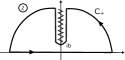
Figure 1: Contour of integration $C_{+}$ used in integral Eq. (64). There is a branch cut from $ib$ to $i\infty$.

Then

$$I_{+}=\int_{-\infty}^{+\infty}\frac{e^{i2\pi(z+f)}}{\sqrt{z^{2}+b^{2}}}dz+\int_{i\infty}^{ib}\frac{e^{i2\pi(z+f)}}{\sqrt{(z+0)^{2}+b^{2}}}dz+\int_{ib}^{i\infty}\frac{e^{i2\pi(z+f)}}{\sqrt{(z-0)^{2}+b^{2}}}dz=0,$$ (65)

and the integrals over the arcs vanished due to their exponential decay as the radius goes to infinity. In the expression above notation $\pm 0$ should be understood from which side of the real axis, positive or negative, the variable $z$ approaches zero. This is needed to pick the correct list of the multivalued square root. Therefore,

$$\int_{-\infty}^{+\infty}\frac{e^{i2\pi(z+f)}}{\sqrt{z^{2}+b^{2}}}dz =-\int_{i\infty}^{ib}\frac{e^{i2\pi(z+f)}}{\sqrt{(z+0)^{2}+b^{2}}}dz-\int_{ib}^{i\infty}\frac{e^{i2\pi(z+f)}}{\sqrt{(z-0)^{2}+b^{2}}}dz$$ (66)

$$=i\int_{b}^{\infty}\frac{e^{i2\pi f-2\pi z}}{\sqrt{-(z-i0)^{2}+b^{2}}}dz-i\int_{b}^{\infty}\frac{e^{i2\pi f-2\pi z}}{\sqrt{-(z+i0)^{2}+b^{2}}}dz$$ (67)

$$=2e^{i2\pi f}\int_{b}^{\infty}\frac{e^{-2\pi z}}{\sqrt{z^{2}-b^{2}}}dz$$ (68)

$$=2e^{i2\pi f}\int_{1}^{\infty}\frac{e^{-2\pi bz}}{\sqrt{z^{2}-1}}dz$$ (69)

$$=2e^{i2\pi f}e^{-2\pi b}\int_{0}^{\infty}\frac{e^{-2\pi bz}}{\sqrt{z(z+2)}}dz$$ (70)

$$\approx 4e^{i2\pi f}e^{-2\pi b}\mathrm{arcsinh}\left(\sqrt{\frac{1}{4\pi b}}\right)$$ (71)

$$=4e^{i2\pi f}e^{-2\pi b}\ln\left(\sqrt{\frac{1}{4\pi b}}+\sqrt{\frac{1}{4\pi b}+1}\right).$$ (72)

Therefore,

$$2\int_{-\infty}^{+\infty}\frac{\cos(2\pi(x+f))}{\sqrt{x^{2}+b^{2}}}dx=8\cos(2\pi f)e^{-2\pi b}\ln\left(\sqrt{\frac{1}{4\pi b}}+\sqrt{\frac{1}{4\pi b}+1}\right)$$ (73)

$$1=2U\left\{2\ln\left[\frac{2\sqrt{(\Lambda-f)f}}{b}\right]+8\cos(2\pi f)e^{-2\pi b}\ln\left(\sqrt{\frac{1}{4\pi b}}+\sqrt{\frac{1}{4\pi b}+1}\right)\right\},$$ (74)

where we remind that $b=\frac{2\theta}{B}$.

.2.1 $8\pi\frac{\theta}{B}>1$ case

In this case we expand the logarithm as

$$2\int_{-\infty}^{+\infty}\frac{\cos(2\pi(x+f))}{\sqrt{x^{2}+b^{2}}}dx=8\cos(2\pi f)e^{-2\pi b}\sqrt{\frac{1}{4\pi b}}.$$ (75)

This is now a small correction to the non-linear equation Eq. (74),

$$1=4U\left\{\ln\left[\frac{\sqrt{(\Lambda-f)fB^{2}}}{\theta}\right]+4\cos(2\pi f)e^{-4\pi\frac{\theta}{B}}\sqrt{\frac{B}{8\pi\theta}}\right\},$$ (76)

and can be treated perturbatively. Assume we found

$$1=4U\ln\left[\frac{\sqrt{(\Lambda-f)fB^{2}}}{\theta}\right],$$ (77)

which is

$$\theta_{0}=\sqrt{\mu^{2}-\frac{B^{2}}{4}}e^{-\frac{1}{4U}},$$ (78)

where $fB=\mu-\frac{B}{2}$, and where we set $\Lambda-\mu=\mu$ in order to make sure that the magnetization is absent when the magnetic field is zero, i.e. there is no spontaneous magnetic order in the system. We comment on that in more details in the subsection C.

In order to find oscillating part of the hybridization we perturb $\theta=\theta_{0}+\delta\theta$ and get

$$\delta\theta=2\theta_{0}\cos\left(2\pi\frac{\mu}{B}-\pi\right)e^{-4\pi\frac{\theta_{0}}{B}}\sqrt{\frac{B}{2\pi\theta_{0}}},$$ (79)

and the solution reads

$$\theta=\theta_{0}+2\theta_{0}\cos\left(2\pi\frac{\mu}{B}-\pi\right)e^{-4\pi\frac{\theta_{0}}{B}}\sqrt{\frac{B}{2\pi\theta_{0}}}.$$ (80)

.2.2 $8\pi\frac{\theta}{B}\sim 1$ case

For example, we keep in mind a situation when $b=0.1$, then $4\pi b=8\pi\frac{\theta}{B}\approx 1.2$. Then, we estimate last term in the brackets in the right-hand side of Eq. (74) to be

$$4e^{-2\pi b}\ln\left(\sqrt{\frac{1}{4\pi b}}+\sqrt{\frac{1}{4\pi b}+1}\right)\approx 1.6,$$ (81)

which is still a small correction as compared to the first term in the brackets of the right-hand side of Eq. (74). We just can not expand the logarithm anymore. We get the solution

$$\theta=\theta_{0}+4\theta_{0}\cos\left(2\pi\frac{\mu}{B}-\pi\right)e^{-4\pi\frac{\theta_{0}}{B}}\ln\left(\sqrt{\frac{B}{8\pi\theta_{0}}}+\sqrt{\frac{B}{8\pi\theta_{0}}+1}\right).$$ (82)

.2.3 $8\pi\frac{\theta}{B}<1$ case

The non-linear equation reads

$$1=2U\left\{2\ln\left[\frac{2\sqrt{(\Lambda-f)f}}{b}\right]+4\cos(2\pi f)e^{-2\pi b}\ln\left(\frac{1}{\pi b}\right)\right\},$$ (83)

where, recall $b=\frac{2\theta}{B}$ and $fB=\mu-\frac{B}{2}$, and $B\Lambda=2\mu$ to make sure there is no spontaneous magnetization in the system. We then derive a solution for the hybridization,

$$\theta=\sqrt{\mu^{2}-\frac{B^{2}}{4}}e^{-\frac{1+8U\cos\left(2\pi\frac{\mu}{H}-\pi\right)e^{-4\pi\frac{\theta}{B}}\ln\left[\pi\frac{\sqrt{4\mu^{2}-B^{2}}}{B}\right]}{4U\left[1+2\cos\left(2\pi\frac{\mu}{B}-\pi\right)e^{-4\pi\frac{\theta}{B}}\right]}}.$$ (84)

When $\cos\left(2\pi\frac{\mu}{B}-\pi\right)=0$, the gap is

$$\theta=\sqrt{\mu^{2}-\frac{B^{2}}{4}}e^{-\frac{1}{4U}}.$$ (85)

Moreover, it is clear that the solution is on the boarderline of its existance. Namely, when the sign of the argument of the natural exponent changes sign to positive, the solution no longer obeys $8\pi\frac{\theta}{B}<1$ and $\theta<\mu$ smallness conditions which were assumed in the course of the derivation. Even next harmonics of the oscillation which were omitted in the calculation can’t help the argument to not change the sign to positive. Hence, large magnetic fields causes a phase transition by either closing the gap or changing the solution to another limit, i.e. to $8\pi\frac{\theta}{B}>1$ case, when the oscillations are rather suppressed and the argument changes sign back to negative. It is quite likely this process is accompanied with a phase separation of the two possibilities. We anticipate that the oscillations are going to be antisymmetric with respect to highest and lowest phases of the oscillation, besides the existence of the higher harmonics which become less exponentially suppressed.

.3 Free energy and magnetization

Here we wish to derive the free energy $F$ within the Keldysh technique. We will be following Ref. [2SM].

$$F=U-TS,$$ (86)

where $S=\int dT\frac{1}{T}\frac{dU}{dT}$ is entropy, and the internal energy $U$ is typically $U=\int_{\epsilon}{\cal F}_{\epsilon}A_{\epsilon}$, where $A_{\epsilon}$ is a function of $\epsilon$ and ${\cal F}_{\epsilon}=\tanh\left(\frac{\epsilon}{2T}\right)$ is the distribution function, then

$$S=\frac{1}{T}\int_{\epsilon}A_{\epsilon}{\cal F}_{\epsilon}-\frac{1}{T}\int_{\epsilon}A_{\epsilon}\left[1+\frac{2T}{\epsilon}\ln\left(1+e^{-\frac{\epsilon}{T}}\right)\right],$$ (87)

and therefore,

$$F=\int_{\epsilon}A_{\epsilon}\left[1+\frac{2T}{\epsilon}\ln\left(1+e^{-\frac{\epsilon}{T}}\right)\right]\rightarrow\int_{\epsilon}A_{\epsilon}\frac{2T}{\epsilon}\ln\left(1+e^{-\frac{\epsilon}{T}}\right).$$ (88)

Here $1$ in the square brackets should be dropped in order to define a proper free energy, hence the right arrow. Then we can define the free energy by figuring out the internal energy, which can be done within the Keldysh technique. For that, following the lines of Ref. [2SM], we introduce heat density sources in to the action.

$$iS_{\eta}+iS_{0}+iS_{\mathrm{int},1}+iS_{\mathrm{int};2}=$$ (89)

$$\frac{i}{2}\int_{t,{\bf r}}\left\{i{\bar{\Psi}}(x)\frac{1}{1+\hat{\eta}}\partial_{t}\Psi(x)-i\left[\partial_{t}{\bar{\Psi}}(x)\right]\frac{1}{1+\hat{\eta}}\Psi(x)\right\}$$ (90)

$$+i\int_{t,{\bf r}}\left\{\hat{\bar{\Psi}}(x)\hat{\sigma}_{0}\left[\begin{array}[]{cc}-\hat{\xi}_{\bf k}&0\\ 0&-\epsilon_{0}\end{array}\right]\hat{\Psi}(x)+\hat{\bar{\Psi}}(x)\left[\begin{array}[]{cc}0&-\theta\hat{\sigma}_{0}-\theta_{\mathrm{q}}\hat{\sigma}_{1}\\ -\theta\hat{\sigma}_{0}-\bar{\theta}_{\mathrm{q}}\hat{\sigma}_{1}&0\end{array}\right]\frac{1}{1+\hat{\eta}}\hat{\Psi}(x)\right\}$$ (95)

$$-\frac{i}{2}\int_{t,{\bf r}}\mathrm{Tr}_{\mathrm{K}}\left[\hat{\bar{\theta}}(x)U^{-1}\hat{\sigma}_{1}\frac{1}{1+\hat{\eta}}\hat{\theta}(x)\right],$$ (96)

where $\hat{\eta}=\eta_{1}\hat{\sigma}_{0}+\eta_{2}\hat{\sigma}_{1}$ are the heat density sources, and $\hat{\xi}_{\bf k}$ stands for operator acting on the coordinate. Heat density is given by varying the partition functino with respect to the source,

$$\langle h_{\mathrm{cl}}\rangle=\frac{i}{2}\left.\frac{\delta Z}{\delta\eta_{2}}\right|_{\eta_{1}=\eta_{2}=0}.$$ (97)

Internal energy $U$ is defined by this average. Let us find out what $A_{\epsilon}$ defined in Eq. (88) equals to in our model. After fermions are integrated out

$$iS=\int_{\epsilon}\int_{{\bf k}}\mathrm{Tr}\ln\left[1-\hat{G}\hat{h}_{\mathrm{int};q}-\hat{G}\left[\begin{array}[]{cc}\epsilon&-\theta\\ -\theta&\epsilon\end{array}\right]\hat{\eta}\right],$$ (100)

where $\hat{G}$ and $\hat{h}_{\mathrm{int};q}$ were defined in the subsection .1. Then

$$\frac{i}{2} \left.\frac{\delta}{\delta\eta_{2}}\left(iS_{\eta}+iS_{0}+iS_{\mathrm{int},1}\right)\right|_{\eta_{1}=\eta_{2}=0;\theta_{\mathrm{q}}=0}$$ (101)

$$=\frac{i}{2}(2\pi i)\int_{\epsilon}\int_{\bf k}\left[2\epsilon^{2}-\epsilon(\epsilon_{0}+\xi_{\bf k})-2\theta^{2}\right]\left[\delta(\epsilon-\epsilon_{{\bf k};+})-\delta(\epsilon-\epsilon_{{\bf k};-})\right]\frac{{\cal F}_{\epsilon}}{\epsilon_{{\bf k};+}-\epsilon_{{\bf k};-}}$$ (102)

$$=-\frac{1}{2}\int_{\bf k}\epsilon_{{\bf k};+}{\cal F}_{\epsilon_{{\bf k};+}}-\frac{1}{2}\int_{\bf k}\epsilon_{{\bf k};-}{\cal F}_{\epsilon_{{\bf k};-}}+\theta^{2}\int_{\bf k}\frac{{\cal F}_{\epsilon_{{\bf k};+}}-{\cal F}_{\epsilon_{{\bf k};-}}}{\epsilon_{{\bf k};+}-\epsilon_{{\bf k};-}}$$ (103)

$$=-\frac{1}{2}\int_{\bf k}\epsilon_{{\bf k};+}{\cal F}_{\epsilon_{{\bf k};+}}-\frac{1}{2}\int_{\bf k}\epsilon_{{\bf k};-}{\cal F}_{\epsilon_{{\bf k};-}}+\frac{\theta^{2}}{U},$$ (104)

where in the last equality sign we utilized self-consistent gap equation. Another term reads

$$\frac{i}{2}\left.\frac{\delta}{\delta\eta_{2}}iS_{\mathrm{int},2}\right|_{\eta_{1}=\eta_{2}=0;\theta_{\mathrm{q}}=0}=-\frac{\theta^{2}}{2U}.$$ (105)

Summing the two we get

$$\frac{i}{2} \left.\frac{\delta}{\delta\eta_{2}}\left(iS_{\eta}+iS_{0}+iS_{\mathrm{int},1}+iS_{\mathrm{int},2}\right)\right|_{\eta_{1}=\eta_{2}=0;\theta_{\mathrm{q}}=0}=-\frac{1}{2}\int_{\bf k}\epsilon_{{\bf k};+}{\cal F}_{\epsilon_{{\bf k};+}}-\frac{1}{2}\int_{\bf k}\epsilon_{{\bf k};-}{\cal F}_{\epsilon_{{\bf k};-}}+\frac{\theta^{2}}{2U},$$ (106)

which gives the correct expression for the free energy upon calculating entropy.

We study the free energy at $T=0$, it is given by

$$F=\frac{B}{2}\sum_{n}\left(Bn+\frac{B}{2}-\mu\right)-\frac{B}{2}\sum_{n}\sqrt{\left(Bn+\frac{B}{2}-\mu\right)^{2}+4\theta^{2}}+\frac{\theta^{2}}{2U}.$$ (107)

The sum over the Landau levels in the second term will be made again with the help of Poisson summation formula Eq. (61) .

$$F=F_{0}+F_{\Sigma},$$ (108)

$$F_{0}=\frac{1}{2}B^{2}\int_{-f}^{\Lambda-f}zdz-\frac{1}{2}B^{2}\int_{-f}^{\Lambda-f}\sqrt{z^{2}+b^{2}}dz+\frac{\theta^{2}}{2U},$$ (109)

$$F_{\Sigma}=-\frac{1}{2}B^{2}\sum_{p}\int_{-f}^{\Lambda-f}e^{i2\pi p(z+f)}\sqrt{z^{2}+b^{2}}dz.$$ (110)

We calculate

$$F_{0} =\frac{1}{4}\left[(\Lambda-f)^{2}B^{2}-f^{2}B^{2}\right]-\frac{1}{4}\left[(\Lambda-f)^{2}B^{2}+f^{2}B^{2}+4\theta^{2}\right]-\frac{\theta^{2}}{2U}+\frac{\theta^{2}}{2U}$$ (111)

$$=-\frac{1}{2}\left(\mu-\frac{B}{2}\right)^{2}-\theta^{2}$$ (112)

where, recall, $\Lambda B=2\mu$ and $fB=\mu-\frac{B}{2}$. This calculation of the free energy is in line with the BCS theory, i.e the energy gain is equal to $-\theta^{2}$. We note that the response from the non-interacting term (when hybridization is treated as a constant rather than self-consistently) is diamagnetic, although it is not immediately clear from Eq. (112).

Now the sum over the harmonics. We again pick only $p=\pm 1$ from the sum. Then we are left with the integral, which in the small magnetic field regime, i.e. $\frac{1}{2\pi b}<1$, is estimated to be

$$\int_{-\infty}^{+\infty}\sqrt{z^{2}+b^{2}}e^{i2\pi(z+f)}dz\rightarrow-e^{i2\pi f}e^{-2\pi b}\frac{4bB^{2}}{\pi}\sqrt{\frac{1}{4\pi b}\left(1+\frac{1}{4\pi b}\right)},$$ (113)

where by $\rightarrow$ we extracted only oscillating part, and we remind $b=\frac{2\theta_{0}}{B}$. We used integration by parts once in order to get rid of divergence at infinity. After that we utilized the same contour integration as was used in Eq. (66). Therefore, for $4\pi b>1$ we get for the oscillating part of free energy,

$$F_{\Sigma} =-B^{2}\int_{-\infty}^{+\infty}\sqrt{z^{2}+b^{2}}\cos(2\pi(z+f))dx\rightarrow\frac{B^{2}}{\pi^{2}}\sqrt{\frac{2\pi\theta_{0}}{B}}\cos\left(2\pi\frac{\mu}{B}-\pi\right)e^{-4\pi\frac{\theta_{0}}{B}}.$$ (114)

Oscillating term from $-\theta^{2}$ is obtained by plugging in Eq. (80) there,

$$F_{0}=-\theta^{2}\approx-\theta_{0}^{2}-4\theta_{0}^{2}\cos\left(2\pi\frac{\mu}{B}-\pi\right)e^{-4\pi\frac{\theta_{0}}{B}}\sqrt{\frac{B}{2\pi\theta_{0}}}.$$ (115)

Here is why we have been choosing $\Lambda B=2\mu$ in all of our calculations. The non-oscillating part of the free energy obtained from Eq. (115) reads $-\theta_{0}^{2}=-\left(\mu^{2}-\frac{B^{2}}{4}\right)e^{-\frac{1}{2U}}$, and hence there is no term here propotional to the magnetic field in free energy. If there was a term propotional to the magnetic field, the system would have had a spontaneous magnetization, which is experimentally not the case. We also conclude from this argument that the response of the system is diamagnetic, because non-oscillating part of the magnetization is $M_{0}=-\partial_{B}(-\theta_{0}^{2})=-\frac{B}{2}e^{-\frac{1}{2U}}$. The system wants to expel the magnetic field such that the Coulomb energy of the system is minimized.

We compare now the two oscillating terms in the free energy, the one came from Eq. (112), which is due to the Coulomb interaction, and the other from the non-interacting picture given by Eq. (114),

$$\delta F_{\mathrm{osc}}=-4\theta_{0}^{2}\sqrt{\frac{B}{2\pi\theta_{0}}}\left(1-\frac{B}{2\pi\theta_{0}}\right)\cos\left(2\pi\frac{\mu}{B}-\pi\right)e^{-4\pi\frac{\theta_{0}}{B}}.$$ (116)

Oscillating part of the magnetization reads

$$M_{\mathrm{osc}}=-\frac{\partial\delta F_{\mathrm{osc}}}{\partial B}\approx-\frac{\mu}{\pi\theta_{0}}\left(\frac{2\pi\theta_{0}}{B}\right)^{\frac{3}{2}}\left(1-\frac{B}{2\pi\theta_{0}}\right)\sin\left(2\pi\frac{\mu}{B}-\pi\right)e^{-4\pi\frac{\theta_{0}}{B}},$$ (117)

where only the $\propto\mu$ term was kept because it is the largest parameter here. Clearly, the non-interacting term which is second in the brackets is subleading in the case of small magnetic fields, $\frac{B}{2\pi\theta_{0}}<1$. Recall, that we have assumed $\frac{B}{8\pi\theta_{0}}<1$ in our derivations. The amplitude vanishes at $\frac{B}{2\pi\theta_{0}}=1$, and at higher fields the non-interacting term will dominate. It is not surprising as in this limit the field becomes larger than the hybridization gap and the system can be thought of as metallic. Even so, in this limit, $\frac{B}{8\pi\theta_{0}}>1$, we have predicted formation of the orbital domains due to the Coulomb interaction.

.3.1 Comment on the Ref. [3SM] A. Allocca and N. Cooper, SciPost Phys. 12, 123 (2022)

Although self-consistent equation on the hybdridization was utilized in Ref. [3SM] and there is a correspondence of their intermediate steps with the steps made in the present paper till the Eq. (13), however, further predictions and conclusions reached in Ref. [3SM] are different from the ones obtained in the present paper. Importantly, contrary to what is found here, the contribution to the dHvA effect from the magnetic field dependence of the hybridization is claimed in Ref. [3SM] to have the same field dependence as the non-interacting part found in Ref. KnolleCooperPRL15 of the Main Text. Whereas in the present paper it is found to be the dominant contribution at small magnetic fields as compared to the non-interacting part. Moreover, present paper predicts that the amplitude of the dHvA oscillations vanishes at $B=2\pi\theta_{0}$ (similar to beating). Ref. [3SM] does not have any discussion on the temperature dependence of the effect. In addition, the higher harmonics of dHvA osillation are found here to be exponentially suppressed as expected, contrary to what is claimed in Ref. [3SM].

.4 Temperature dependence

Here we study temperature dependence of oscillations obtained in previous subsections. For that we update the non-linear equation to account for the temperature,

$$1=UB\sum_{n}\frac{{\cal F}_{\epsilon_{n,+}}-{\cal F}_{\epsilon_{n,-}}}{\sqrt{(Bn+\frac{B}{2}-\mu)^{2}+4\bar{\theta}\theta}}$$ (118)

We follow the same steps as were in $T=0$ case. In case of finite temperature the integral Eq. (62) gets modified as

$$\int_{0}^{\Lambda}\frac{dx}{\sqrt{(x-f)^{2}+b^{2}}}\rightarrow\int_{-f}^{\Lambda-f}\frac{dz}{\sqrt{z^{2}+b^{2}}}\left[1-\frac{1}{e^{\frac{-z+\sqrt{z^{2}+b^{2}}}{2T/B}}+1}-\frac{1}{e^{\frac{z+\sqrt{z^{2}+b^{2}}}{2T/B}}+1}\right]dz$$ (119)

This is because ${\cal F}_{x}=1-\frac{2}{e^{\frac{x}{T}}+1}$. Here, again $b=\frac{2\theta_{0}^{2}}{B}$ and $f=\frac{\mu}{B}-\frac{1}{2}$. We plot temperature dependence of the last two terms in the square brackets in the right hand side of Eq. (119) in Fig. In addition, let us do some analytics

$$-\int_{-f}^{\Lambda-f}\frac{dz}{\sqrt{z^{2}+b^{2}}}\left[\frac{1}{e^{\frac{-z+\sqrt{z^{2}+b^{2}}}{2T/B}}+1}+\frac{1}{e^{\frac{z+\sqrt{z^{2}+b^{2}}}{2T/B}}+1}\right]dz$$ (120)

$$=-\left.\frac{1}{2}\ln\left[\frac{z+\sqrt{z^{2}+b^{2}}}{\sqrt{z^{2}+b^{2}}-z}\right]\left[\frac{1}{e^{\frac{-z+\sqrt{z^{2}+b^{2}}}{2T/B}}+1}+\frac{1}{e^{\frac{z+\sqrt{z^{2}+b^{2}}}{2T/B}}+1}\right]\right|_{-f}^{\Lambda-f}$$ (121)

$$+\frac{1}{2}\int_{-f}^{\Lambda-f}dz\ln\left[\frac{z+\sqrt{z^{2}+b^{2}}}{\sqrt{z^{2}+b^{2}}-z}\right]\partial_{z}\left[\frac{1}{e^{\frac{-z+\sqrt{z^{2}+b^{2}}}{2T/B}}+1}+\frac{1}{e^{\frac{z+\sqrt{z^{2}+b^{2}}}{2T/B}}+1}\right]$$ (122)

$$\approx-2\ln\left[\frac{2\sqrt{(\Lambda-f)f}}{b}\right]\frac{1}{e^{\frac{Bb^{2}}{4Tf}}+1}$$ (123)

$$=-2\ln\left[\frac{\sqrt{\mu^{2}-\frac{B^{2}}{4}}}{\theta_{0}}\right]\frac{1}{e^{\frac{\theta_{0}^{2}}{T\mu}}+1},$$ (124)

where we kept only Eq. (121) after integrating by parts, as the other is less singular at $z=0$, and assumed $\Lambda-f\approx f$ in the distribution function when taking the upper and lower limits. This assumption is valid at small temperatures, when the derivative over the distribution function is almost a delta function. The upper and lower limits are fixed and are never equal to infinity.

Now, the most interesting part. The integral corresponding to oscillations at zero temperature Eq. (66) gets modified as

$$\int_{-\infty}^{+\infty}\frac{e^{i2\pi(z+f)}}{\sqrt{z^{2}+b^{2}}}dz\rightarrow\int_{-\infty}^{+\infty}\frac{e^{i2\pi(z+f)}}{\sqrt{z^{2}+b^{2}}}\left[1-\frac{1}{e^{\frac{-z+\sqrt{z^{2}+b^{2}}}{2T/B}}+1}-\frac{1}{e^{\frac{z+\sqrt{z^{2}+b^{2}}}{2T/B}}+1}\right]dz.$$ (125)

Let us work with the temperature dependent parts only. We define the $+1$ harmonic to be

$${\cal R}^{(+1)}_{\mathrm{osc}}(T)= \int_{-\infty}^{+\infty}\frac{e^{i2\pi(z+f)}}{\sqrt{z^{2}+b^{2}}}\left[1-\frac{1}{e^{\frac{-z+\sqrt{z^{2}+b^{2}}}{2T/B}}+1}-\frac{1}{e^{\frac{z+\sqrt{z^{2}+b^{2}}}{2T/B}}+1}\right]dz$$ (126)

$$= e^{i2\pi f}\int_{-\infty}^{+\infty}e^{i2\pi b\sinh(y)}\left[1-\frac{1}{e^{\frac{\theta_{0}}{T}e^{-y}}+1}-\frac{1}{e^{\frac{\theta_{0}}{T}e^{y}}+1}\right]dy$$ (127)

$$\equiv e^{i2\pi f}\left(W_{-}+W_{+}\right),$$ (128)

where we made $z=b\sinh(y)$ change of variable, which resulted in $dz=b\cosh(y)dy$, $\sqrt{z^{2}+b^{2}}=b\cosh(y)$ and $-z+\sqrt{z^{2}+b^{2}}=be^{-y}$ while $z+\sqrt{z^{2}+b^{2}}=be^{y}$, and $\frac{Bb}{2T}=\frac{\theta_{0}}{T}$. Harmonic with $-1$ is obtained from Eq. (126) by complex conjugation, i.e. ${\cal R}^{(-1)}_{\mathrm{osc}}(T)=\left[{\cal R}^{(+1)}_{\mathrm{osc}}(T)\right]^{*}$.

Figure 3: Contour of integration used to calculate $W_{-}$ defined in Eq. (127) and Eq. (129). The contour is closed on the top part of the complex plane in order to ensure convergence. The residues are picked from inside of the contour.

We introduce contour integration shown in Fig. (3) and obtain the expression for $W_{-}$ defined in Eq. (127),

$$W_{-} =\int_{-\infty}^{+\infty}e^{i2\pi b\sinh(y)}\left[\frac{1}{2}-\frac{1}{e^{\frac{\theta_{0}}{T}e^{-y}}+1}\right]dy$$ (129)

$$=\frac{1}{2}\int_{-\infty}^{+\infty}e^{i2\pi b\sinh(y)}\frac{e^{\frac{\theta_{0}}{T}e^{-y}}-1}{e^{\frac{\theta_{0}}{T}e^{-y}}+1}dy$$ (130)

$$=2\pi i\sum_{\mathrm{res}}(...).$$ (131)

We found it better to come back to $\tanh$ in order to take care of the divergence at infinity. The chosen contour of integration shown in Fig. (3) is such that the integral over the arc converges because of the exponent in the numerator of the integrand in Eq. (129). The residues of the integrand of $W_{-}$ are at $y=y_{n}$ and defined as

$$e^{-y_{n}}=2\pi i\frac{T}{\theta_{0}}\left(n+\frac{1}{2}\right),$$ (132)

and according to the contour Fig. (3) they are with $n<0$, such that $\mathrm{Im}[y_{n}]>0$ and real part can be of any sign. Then

$$i\sinh(y_{n})=\frac{1}{2}\left[\frac{1}{2\pi\frac{T}{\theta_{0}}\left(n+\frac{1}{2}\right)}+2\pi\frac{T}{\theta_{0}}\left(n+\frac{1}{2}\right)\right],$$ (133)

$$\left.\partial_{y}e^{\frac{\theta_{0}}{T}e^{-y}}\right|_{y=y_{n}}=2\pi i\left(n+\frac{1}{2}\right).$$ (134)

$$\frac{1}{2}\left(e^{\frac{\theta_{0}}{T}e^{-y_{n}}}-1\right)=-1.$$ (135)

Then

$$W_{-}=2\pi i\sum_{\mathrm{res}}(...) =-\sum_{n<0}\frac{1}{n+\frac{1}{2}}e^{\pi b\left[\frac{1}{2\pi\frac{T}{\theta_{0}}\left(n+\frac{1}{2}\right)}+2\pi\frac{T}{\theta_{0}}\left(n+\frac{1}{2}\right)\right]}$$ (136)

$$=\sum_{n\geq 0}\frac{1}{n+\frac{1}{2}}e^{-\pi b\left[\frac{1}{2\pi\frac{T}{\theta_{0}}\left(n+\frac{1}{2}\right)}+2\pi\frac{T}{\theta_{0}}\left(n+\frac{1}{2}\right)\right]}.$$ (137)

It is not clear how to analytically sum up the series above, however, in order to gain some insight, we can approximate the series by applying the Poisson summation formula and performing the steepest descent method. We can then numerically plot the result of summation and compare it with the approximate analytics. Before doing it, as a remark, let us contrast with the standard Lifshits-Kosevich expression for the temperature dependence.

.4.1 Poisson summation and steepest descent method

To sum the series Eq. (137) we again employ Poisson summation formula Eq. (61).

$$W_{-} =\sum_{n\geq 0}\frac{1}{n+\frac{1}{2}}e^{-\pi b\left[\frac{1}{2\pi\frac{T}{\theta_{0}}\left(n+\frac{1}{2}\right)}+2\pi\frac{T}{\theta_{0}}\left(n+\frac{1}{2}\right)\right]}$$ (138)

$$=\int_{0}^{\infty}\frac{1}{x+\frac{1}{2}}e^{-\pi b\left[\frac{1}{2\pi\frac{T}{\theta_{0}}\left(x+\frac{1}{2}\right)}+2\pi\frac{T}{\theta_{0}}\left(x+\frac{1}{2}\right)\right]}dx+\sum_{n\neq 0}\int_{0}^{\infty}\frac{e^{i2\pi nx}}{x+\frac{1}{2}}e^{-\pi b\left[\frac{1}{2\pi\frac{T}{\theta_{0}}\left(x+\frac{1}{2}\right)}+2\pi\frac{T}{\theta_{0}}\left(x+\frac{1}{2}\right)\right]}dx$$ (139)

$$\equiv R_{0}(T)+R_{1}(T)+R_{-1}(T)+....$$ (140)

The non-oscillating part of the formula reads

$$R_{0}(T)=\int_{0}^{+\infty}\frac{dx}{x+\frac{1}{2}}e^{-\pi b\left[\frac{1}{2\pi\frac{T}{\theta_{0}}\left(x+\frac{1}{2}\right)}+2\pi\frac{T}{\theta_{0}}\left(x+\frac{1}{2}\right)\right]},$$ (141)

we numerically estimate it and plot it as a function of temperature in Fig. (4).

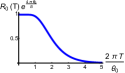
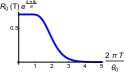
Figure 4: Plot of the numerically estimated expression Eq. (141), left for $b=\frac{2\theta_{0}}{B}=1$, center for $b=\frac{2\theta_{0}}{B}=2$, and right for $b=\frac{2\theta_{0}}{B}=0.2$. It is consistent with standard Lifshits-Kosevich structure.

We can estimate the integral using steepest descent method,

$$R_{0}^{\mathrm{sd}}(T)=\frac{1}{\frac{\theta_{0}}{2\pi T}\bar{z}}e^{-\pi b\left(\frac{1}{\bar{z}}+\bar{z}\right)}\int_{0}^{+\infty}e^{-\frac{1}{2}|g(\bar{z})|\left(x+\frac{1}{2}-\frac{\theta_{0}}{2\pi T}\bar{z}\right)^{2}}dx,$$ (142)

where we defined

$$\bar{z}=\sqrt{\left(\frac{1}{2\pi b}\right)^{2}+1}-\frac{1}{2\pi b}=\frac{2\pi b}{1+\sqrt{1+(2\pi b)^{2}}},$$ (143)

$$g(\bar{z})=\left(\frac{2\pi T}{\theta_{0}}\right)^{2}\left.\partial^{2}_{z}\left[-\ln(z)-\pi b\left(\frac{1}{z}+z\right)\right]\right|_{z=\bar{z}}=\left(\frac{2\pi T}{\theta_{0}}\right)^{2}\left(\frac{1}{\bar{z}^{2}}-2\pi b\frac{1}{\bar{z}^{3}}\right).$$ (144)

In Fig. (5) we plot justification for the steepest descent method. The original curve is plotted in blue, while the curve corresponding to the steepest descent approximation is shown in red. This figure suggests that the position of the extremum is captured correctly, but for large magnetic fields (right plot in Fig. (5)) the approximation only qualitatively describes the integral. We will show in the following that the position of the extremum defines period of quantum oscillations with inverse temperature.

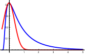
Figure 5: Approximating the integral within the steepest descent method. Left: for $\frac{2\theta_{0}}{B}=1$ and $2\pi\frac{T}{\theta_{0}}=1$. Right: for $\frac{2\theta_{0}}{B}=0.2$ and $2\pi\frac{T}{\theta_{0}}=1$. Red curve is the Gaussian obtained within the steepest descent method, while blue corresponds to the original curve. In both cases the position of the saddle, which defines oscillations with inverse temperature, is perfectly approximated. For large magnetic fields corresponding to the right plot, steepest descent method does not do a good job approximating the magnitude of the integral. It works well for small magnetic fields corresponding to the left plot.

(i) We first consider $2\pi b>1$ case. The steepest descent approximation is shown in the left plot in Fig. (5). Then $\bar{z}\approx 1$ and $|g(1)|=2\pi b\left(\frac{2\pi T}{\theta_{0}}\right)^{2}$, and we get

$$R_{0}^{\mathrm{sd}}(T)=\frac{2\pi T}{\theta_{0}}e^{-2\pi b}\int_{0}^{+\infty}e^{-\pi b\left(\frac{2\pi T}{\theta_{0}}\right)^{2}\left(x+\frac{1}{2}-\frac{\theta_{0}}{2\pi T}\right)^{2}}dx,$$ (145)

which we plot in Fig. (4). At $T=0$ the integral over $x$ can be approximated as Gaussian, i.e. from $-\infty$ to $+\infty$ in our case by shifting $x\rightarrow x+\frac{1}{2}-\frac{\theta_{0}}{2\pi T}$ and setting $-\infty$ in the lower limit, then

$$R_{0}^{\mathrm{sd}}(T=0)\approx\frac{e^{-2\pi b}}{\sqrt{b}}.$$ (146)

At $T\rightarrow\infty$

$$R_{0}^{\mathrm{sd}}(T\rightarrow\infty)\approx\frac{e^{-2\pi b}}{2\sqrt{b}}\mathrm{Erfc}\left(\sqrt{\pi b}\frac{2\pi T}{\theta_{0}}\frac{1}{2}\right)\approx\frac{\theta_{0}}{2\pi T}\frac{e^{-2\pi b}}{\pi b}e^{-\frac{\pi b}{4}\left(\frac{2\pi T}{\theta_{0}}\right)^{2}},$$ (147)

where is the complimentary error function, whose expansion at large values of argument we used.

Now we pick the $\pm n$ harmonics in the formula Eq. (61),

$$R_{+n}(T)+R_{-n}(T) =\int_{0}^{+\infty}e^{i2\pi nx}\frac{1}{x+\frac{1}{2}}e^{-\pi b\left[\frac{1}{2\pi\frac{T}{\theta_{0}}\left(x+\frac{1}{2}\right)}+2\pi\frac{T}{\theta_{0}}\left(x+\frac{1}{2}\right)\right]}dx+\mathrm{c.c.}$$ (148)

$$\approx\frac{1}{\frac{\theta_{0}}{2\pi T}\bar{z}}e^{-\pi b\left(\frac{1}{\bar{z}}+\bar{z}\right)}\int_{0}^{+\infty}e^{i2\pi nx}e^{-\frac{1}{2}|g(\bar{z})|\left(x+\frac{1}{2}-\frac{\theta_{0}}{2\pi T}\bar{z}\right)^{2}}dx+\mathrm{c.c.}$$ (149)

$$=\frac{1}{\frac{\theta_{0}}{2\pi T}\bar{z}}e^{-\pi b\left(\frac{1}{\bar{z}}+\bar{z}\right)}e^{-\frac{2\pi^{2}n^{2}}{|g(\bar{z})|}}e^{in\left(\frac{\theta_{0}}{T}\bar{z}-\pi\right)}\int_{0}^{+\infty}e^{-\frac{1}{2}|g(\bar{z})|\left(x+\frac{1}{2}-\frac{\theta_{0}}{2\pi T}\bar{z}-i\frac{2\pi n}{|g(\bar{z})|}\right)^{2}}dx+\mathrm{c.c.}$$ (150)

$$=2\cos\left[n\left(\frac{\theta_{0}}{T}\bar{z}-\pi\right)\right]e^{-\frac{2\pi^{2}n^{2}}{|g(\bar{z})|}}R_{0}^{\mathrm{sd}}(T).$$ (151)

Since steepest descent method gives $\bar{z}=1$, we predict that there is a peak in $R(T)$ which occurs at

$$T_{\mathrm{peak}}=\frac{\theta_{0}}{\pi}.$$ (152)

In Fig. (6) we plot $R(T)$ for $b=1$, $b=3$ and $b=4$. There the peak indeed occurs at a value determined in Eq. (152).

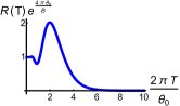
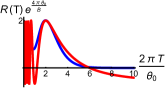
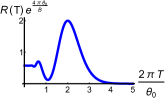
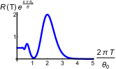
Figure 6: Top row, left: plot of the expression Eq. (137) times $e^{2\pi b}$ factor for $b=\frac{2\theta_{0}}{B}=1$. Top row, right: the same but with $\left[1-2\cos\left(\frac{\theta_{0}}{T}\right)\right]\frac{2}{3}$ (red) plotted together. Now goes a proof of principle. Bottom row, left is the plot of the expression Eq. (137) for $b=\frac{2\theta_{0}}{B}=3$. Bottom row, right is the plot of the expression Eq. (137) for $b=\frac{2\theta_{0}}{B}=4$. The magnitude more and more exponentially suppressed but with that more oscillation cycles, as compared with the first one if going from large temperatures, become visible. In all of the figures the height of the peak equals to approximately $2$ (not universal).

Let us estimate the height of the peak. Numerics suggest, see Fig. (6), that the peak has a value of almost $2e^{-2\pi b}$, let us show it is indeed the case. We found it convenient to not perform the steepest descent for this task, but rather do the following transformations after application of the Poisson summation formula,

$$R(T_{\mathrm{peak}})= \sum_{n}\int_{0}^{+\infty}e^{i2\pi nx}\frac{1}{x+\frac{1}{2}}e^{-\pi b\left[\frac{1}{2\pi\frac{T_{\mathrm{peak}}}{\theta_{0}}\left(x+\frac{1}{2}\right)}+2\pi\frac{T_{\mathrm{peak}}}{\theta_{0}}\left(x+\frac{1}{2}\right)\right]}dx$$ (153)

$$=\sum_{n}e^{-i\pi n}\int_{\ln\left(2\pi\frac{T_{\mathrm{peak}}}{\theta_{0}}\frac{1}{2}\right)}^{+\infty}e^{in\frac{\theta_{0}}{T_{\mathrm{peak}}}e^{z}}e^{-2\pi b\cosh(z)}dz$$ (154)

$$=\sum_{n}e^{-i\pi n}\int_{0}^{+\infty}e^{in\pi e^{z}}e^{-2\pi b\cosh(z)}dz,$$ (155)

now goes our approximation, because $\cosh(z)$ has a minimum at $z=0$ (reminiscent of steepest descent approximation made above), $e^{z}\sim 1+z$ in the vicinity of $z=0$. Therefore,

$$\sum_{n}e^{-i\pi n}\int_{0}^{+\infty}e^{in\pi e^{z}}e^{-2\pi b\cosh(z)}dz \approx\sum_{n}\int_{0}^{+\infty}e^{in\pi z}e^{-2\pi b\cosh(z)}dz$$ (156)

$$=2\sum_{m}\int_{0}^{+\infty}\delta(z-m)e^{-2\pi b\cosh(z)}dz$$ (157)

$$=2e^{-2\pi b}+4e^{-2\pi b\cosh(1)}+4e^{-2\pi b\cosh(2)}+..$$ (158)

$$\approx 2e^{-2\pi b}+4e^{-2\pi b(1+0.5)}+4e^{-2\pi b(1+2.75)}.$$ (159)

For $b=1$ we have $4e^{-2\pi b*0.5}\approx 0.17$ and the other terms in the series are practically zero. For $b=3$ we have $4e^{-2\pi b*0.5}\approx 3*10^{-4}$ which is also practically zero. Therefore, we conclude that

$$R(T_{\mathrm{peak}})\approx 2e^{-2\pi b},$$ (160)

which is indeed numerically plotted in Fig. (6), recalling that $b=\frac{2\theta_{0}}{B}$. This result, we remind, is valid for $2\pi b=\frac{4\pi\theta_{0}}{B}>1$.

(ii) Let us now consider $2\pi b\sim 1$ and $2\pi b<1$ cases.

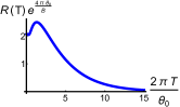
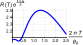
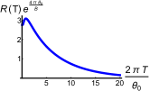
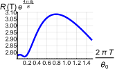
Figure 7: Left: plot of $R(T)e^{\frac{4\pi\theta_{0}}{B}}$ and right is the zoom in in to the peak for an eye determination of the position of the peak. Top is for $\frac{2\theta_{0}}{B}=0.2$ while bottom is for $\frac{2\theta_{0}}{B}=0.1$.

In particular we want to first focus on $b=0.2$ case as we think it might be relevant to the experiment. For this value the steepest descent saddle point is defined by the most general expression,

$$\bar{z}=\frac{2\pi b}{1+\sqrt{1+(2\pi b)^{2}}},$$ (161)

$$g(\bar{z})=\left(\frac{2\pi T}{\theta_{0}}\right)^{2}\left(\frac{1}{\bar{z}^{2}}-2\pi b\frac{1}{\bar{z}^{3}}\right).$$ (162)

Calculations and Fig. (5b) suggest we have to be careful with the steepest descent and take in to account higher orders of approximation. In particular, in Fig. (5b) we see that the position of the saddle point is captured well with the approximation, however, the tail isn’t. The tail is going to contribute to the amplitude of the integral.

$$R_{+n}(T)+R_{-n}(T)\approx 2\cos\left[n\left(2\pi\frac{\theta_{0}^{2}}{HT}-\pi\right)\right]e^{-\frac{2\pi^{2}n^{2}}{|g(\bar{z})|}}R_{0}^{\mathrm{sd}}(T),$$ (163)

the peak occurs at

$$T_{\mathrm{peak}}=\frac{4\theta_{0}^{2}}{H}\frac{1}{{1+\sqrt{1+\left(\frac{4\pi\theta_{0}}{B}\right)^{2}}}}=\frac{4\theta_{0}^{2}}{{B+\sqrt{B^{2}+\left(4\pi\theta_{0}\right)^{2}}}},$$ (164)

which for small values of $\frac{4\pi\theta_{0}}{B}$ becomes $T_{\mathrm{peak}}=\frac{2\theta_{0}^{2}}{B}$. Let us check that our approximation works. From right plots of Fig. (7) we observe that for $\frac{2\theta_{0}}{B}=0.2$ the position of the peak is at $\frac{2\pi T^{(\mathrm{plot})}_{\mathrm{peak}}}{\theta_{0}}\approx 1.32$ which should be compared with the corresponding quantity from the Eq. (164), which is $\frac{2\pi T^{(\mathrm{analytics})}_{\mathrm{peak}}}{\theta_{0}}\approx 0.96$. It turns out that for whatever reason better approximation is $T^{*}_{\mathrm{peak}}=\frac{2\theta_{0}^{2}}{B}$, which gives $\frac{2\pi T^{*}_{\mathrm{peak}}}{\theta_{0}}=2\pi b\approx 1.25$. For $\frac{2\theta_{0}}{B}=0.1$ we have $\frac{2\pi T^{(\mathrm{plot})}_{\mathrm{peak}}}{\theta_{0}}\approx 0.78$ which is compared with $\frac{2\pi T^{(\mathrm{analytics})}_{\mathrm{peak}}}{\theta_{0}}\approx 0.57$ and $\frac{2\pi T^{*}_{\mathrm{peak}}}{\theta_{0}}=2\pi b\approx 0.62$. We conclude that the steepest descent approximation is a poor approximation for $\frac{4\pi\theta_{0}}{B}<1$ case.

.4.2 Conventional Lifshits-Kosevich expression for the temperature dependence

As a remark, let us contrast our calculation with the standard Lifshits-Kosevich expression for the temperature dependence of dHvA oscillation of a metal. There integral defining the temperature dependence of the dHvA oscillation amplitude instead of Eqs. (127), (129), and (137) equals (for example see Ref. [4SM], E.M. Lifshits and L.P. Pitaevskii “Statistical Physics, Part 2: Course of Theoretical Physics - Vol. 9”) to

$$I_{\mathrm{LK}}(\alpha)=\int_{-\infty}^{+\infty}\frac{e^{i\alpha z}}{e^{z}+1},$$ (165)

where $\alpha>0$. The contour of integration is the same as in Fig. (3), and the residues are at $z_{n}=2\pi i\left(n+\frac{1}{2}\right)$ with $n>0$. Then,

$$I_{\mathrm{LK}}(\alpha) =-2\pi i\sum_{n=0}e^{-2\pi\left(n+\frac{1}{2}\right)\alpha}$$ (166)

$$=-2\pi ie^{-\pi\alpha}\sum_{n=0}e^{-2\pi n\alpha}$$ (167)

$$=-\frac{\pi i}{\sinh(\pi\alpha)},$$ (168)

where we used

$$\frac{1}{\sinh(\pi\alpha)}=2e^{-\pi\alpha}\sum_{n=0}e^{-2\pi n\alpha}.$$ (169)

We see that there is no quantum oscillations as a function of temperature in metallic case.

.5 References in Supplemental Material (SM)

1. A. Kamenev, Field theory of non-equilibrium systems (Cambridge, University Press, 2012).

2. G. Schwiete and A.M. Finkel’stein PRB 90, 155441 (2014).

3. A. Allocca and N. Cooper, SciPost Phys. 12, 123 (2022).

4. E.M. Lifshits and L.P. Pitaevskii “Statistical Physics, Part 2: Course of Theoretical Physics - Vol. 9” Elsevier 2014.

References

(1) G. Li, Z. Xiang, F. Yu, T. Asaba, B. Lawson, P. Cai, C. Tinsman, A. Berkley,
S. Wolgast, Y.S. Eo, D.-J. Kim, C. Kurdak, J.W. Allen, K. Sun, X.H. Chen,
Y.Y. Wang, Z. Fisk, and L. Li, Science 346, 1208 (2014).
(2) B.S. Tan, Y.-T. Hsu, B. Zeng, M.C. Hatnean, N. Harrison, Z. Zhu,
M. Hartstein, M. Kiourlappou, A. Srivastava, M.D. Johannes, T.P. Murphy,
J.-H. Park, L. Balicas, G.G. Lonzarich, G. Balakrishnan, and S.E. Sebastian, Science 349, 287 (2015).
(3) M. Hartstein, W.H. Toews, Y.-T. Hsu, B. Zeng, X. Chen, M.C. Hatnean, Q.R. Zhang, S. Nakamura, A.S. Padgett, G. Rodway-Gant, J. Berk, M.K. Kingston, G.H. Zhang, M.K. Chan, S. Yamashita, T. Sakakibara, Y. Takano, J.-H. Park, L. Balicas, N. Harrison, N. Shitsevalova, G. Balakrishnan, G. G. Lonzarich, R. W. Hill, M. Sutherland, and S.E. Sebastian, Nature Physics 14, 166 (2018).
(4) M. Hartstein, H. Liu, Y.-T. Hsu, B.S. Tan, M.C. Hatnean, G. Balakrishnan,
and S.E. Sebastian, iScience 23, 101632 (2020).
(5) G. Baskaran, arXiv: 1507.03477 (2015).
(6) I. Sodemann, D. Chowdhury, and T. Senthil, Phys. Rev. B 97, 045152 (2017).
(7) C.M. Varma, Phys. Rev. B 102, 155145 (2020).
(8) J. Knolle and N.R. Cooper, Phys. Rev. Lett. 115, 146401 (2015).
(9) G. Singh and H. Pal, arXiv: 2210.10475 (2022).
(10) A.C. Hewson ”The Kondo Problem to Heavy Fermions”, Cambridge University Press, 1993.
(11) See Supplemental Material for details.
(12) H. Aoki, N. Kimura, and T. Terashima
Journal of the Physical Society of Japan 83, 072001 (2014).
(13)
Z. Xiang, K.-W. Chen, L. Chen, T. Asaba, Y. Sato, N. Zhang, D. Zhang, Y. Kasahara, F. Iga, W.A. Coniglio, Y. Matsuda, J. Singleton, and L. Li,
Phys. Rev. X 12, 021050 (2022).
(14) D. Xiao, C.-X. Liu, N. Samarth, and L.-H. Hu, Phys. Rev. Lett. 122, 186802 (2019).
(15) Z. Han, T. Li, L. Zhang, G. Sullivan, and R.-R. Du, Phys. Rev. Lett. 123, 126803 (2019).
(16) B.Z. Spivak, A.Yu. Zyuzin, and D.H. Cobden, Phys. Rev. Lett. 95, 226804 (2005).
(17) M. Dzero, K. Sun, V. Galitski, and P. Coleman, Phys. Rev. Lett. 104, 106408 (2010).
(18)B. A. Volkov and O. A. Pankratov, Pis’ma Zh. Eksp. Teor. Fiz.
42, 145 (1985) [JETP Lett. 42, 178 (1985)];
O.A. Pankratov, S.V. Pakhomov, and B.A. Volkov, Solid State Communications, 61, 93 (1987).
(19) A. Allocca and N. Cooper, SciPost Phys. 12, 123 (2022).