CTP-SCU/2023004

Timelike entanglement entropy and $T\bar{T}$ deformation

Xin Jiang^a, Peng Wang^a, Houwen Wu^a,b and Haitang Yang^a

^aCollege of Physics

Sichuan University

Chengdu, 610065, China

^bDAMTP, Centre for Mathematical Sciences

University of Cambridge

Cambridge, CB3 0WA, UK

domoki@stu.scu.edu.cn, pengw@scu.edu.cn, hw598@damtp.cam.ac.uk, hyanga@scu.edu.cn

Abstract

In a previous work [1] about the $T\bar{T}$ deformed CFT₂, from the consistency requirement of the entanglement entropy, we found that in addition to the usual spacelike entanglement entropy, a timelike entanglement entropy must be introduced and treated equally. Motivated by the recent explicit constructions of the timelike entanglement entropy and its bulk dual, we provide a comprehensive analysis of the timelike and spacelike entanglement entropies in the $T\bar{T}$ deformed finite size system and finite temperature system. The results confirm our prediction that in the finite size system only the timelike entanglement entropy receives a correction, while in the finite temperature system only the usual spacelike entanglement entropy gets a correction. These findings affirm the necessity of a complete measure including both spacelike and timelike entanglement entropies.

1 Introduction

Conformal field theories (CFTs) could be deformed by relevant, marginal and irrelevant deformations. Relevant and marginal deformations have been well studied. Though the irrelevant deformations are non-renormalizable and lead no consequence in the IR region, in two-dimensional spacetime, they turn out to be generally under control and even solvable for some particular models. One such solvable irrelevant deformation is the $T\bar{T}$ deformation [2, 3, 4], obtained by turning on a $T\bar{T}$ coupling term

$$\frac{dI_{\text{QFT}}^{\left(\mu\right)}}{d\mu}=\int d^{2}x\,\left(T\bar{T}\right)_{\mu},$$ (1.1)

where the deformation parameter $\mu$ has the $\left[\text{Length}\right]^{2}$ dimension and $\left(T\bar{T}\right)_{\mu}$is defined by the stress tensor of the deformed theory. At the leading order, the deformed theory is given by

$$I_{\text{QFT}}^{\left(\mu\right)}=I_{\text{CFT}}+\mu\int d^{2}x\,\left(T\bar{T}\right)_{\mu=0}+{\mathcal{O}}(\mu^{2}),$$ (1.2)

where $(T\bar{T})_{\mu=0}=\frac{1}{8}\left[T^{\alpha\beta}T_{\alpha\beta}-\left(T_{\alpha}^{\alpha}\right)^{2}\right]$. It is clear that the Lorentz symmetry is preserved but the conformal symmetry is broken in the $T\bar{T}$ deformed theory.

The importance of this model is revived partially by the proposition, given in Ref.[5], that the $\text{AdS}_{3}$ gravity with a Dirichlet boundary at a finite radial distance $r_{c}$, is dual to the $T\bar{T}$ deformed $\text{CFT}_{2}$ living on that Dirichlet boundary. This nontrivial extension of AdS/CFT correspondence [6] is called cutoff-AdS/$T\bar{T}$-deformed-CFT (cAdS/dCFT) correspondence.

In the UV region, out of the many calculable deformed physical quantities, a particularly important one is the entanglement entropy (EE). Until recently, the entanglement entropy is defined only for spacelike intervals. Thereinafter, we will refer the spacelike EE to the usual standard EE. Some progresses on the spacelike EE in the $T\bar{T}$ deformed $\text{CFT}_{2}$ have been achieved in recent years [7, 8, 9].

With the replica trick [10, 11], in Ref.[12], the $T\bar{T}$ deformed spacelike EE was calculated perturbatively for the cylindrical topology. Intriguingly, the $T\bar{T}$ correction to the spacelike EE is dependent on different interpretations of the identical topology. When treat the system as a finite size one, there is no leading correction. But the finite temperature interpretation does receive a leading correction. This indicates that the $T\bar{T}$ correction to the spacelike EE can be observed in the finite temperature system but is invisible in the finite size system. This result obviously conflicts with the fact that the entanglement entropy is a topological quantity. Moreover, without a correction presented in the finite size system, how do we distinguish between the undeformed CFT and the deformed CFT by the entanglement entropy?

To resolve this inconsistency, in a previous paper [1], by noticing the fact that the finite size system and the finite temperature system share the same cylindrical topology under exchanging $t\leftrightarrow x$, we proposed that in addition to the spacelike EE, there should exist a timelike EE for timelike intervals, and the timelike EE should be treated on the same footing as the spacelike EE. We further predicted, as shown in Table 1, the spacelike EE only receives a correction in the $T\bar{T}$ deformed finite temperature system, while the timelike EE only receives a correction in the $T\bar{T}$ deformed finite size system.

	spacelike EE	timelike EE
Finite size		$\checked$
Finite temperature	$\checked$

Table 1: The symbol $\checked$ marks a correction to the entanglement entropy caused by the $T\bar{T}$ deformation.

Remarkably, such a timelike EE has been specifically defined via analytical continuation and the bulk dual has been explicitly provided in Ref.[13, 14, 15, 16] recently. Rather than real-valued as the spacelike EE, the timelike EE is a complex-valued quantity. It is suggested that the timelike EE needs to be correctly understood as a pseudoentropy, which is a non-Hermitian generalization of the usual spacelike EE. Dividing the total system into two subsystems $A$ and $B$, the pseudoentropy is defined by the von Neumann entropy,

$$S_{A}=-\mathrm{Tr}\left[\tau_{A}\log\tau_{A}\right],$$ (1.3)

of the reduced transition matrix

$$\tau_{A}=\mathrm{Tr}_{B}\left[\frac{\left|\psi\right\rangle\left\langle\varphi\right|}{\left\langle\varphi\mid\psi\right\rangle}\right].$$ (1.4)

Here, $\left|\psi\right\rangle$ and $\left|\varphi\right\rangle$ are two different quantum states in the total Hilbert space that is factorized as $\mathcal{H}=\mathcal{H}_{A}\otimes\mathcal{H}_{B}$. As the usual EE, the pseudoentropy could also be captured by the replica method [10, 11] in path integral formalism. Denoting the manifold corresponding to $\left\langle\varphi\mid\psi\right\rangle$ as $\mathcal{M}_{1}$ and the manifold corresponding to $\mathrm{Tr}_{A}\left(\tau_{A}\right)^{n}$ as $\mathcal{M}_{n}$, the $n$-th pseudo Rényi entropy reads

$$S_{A}^{\left(n\right)}=\frac{1}{1-n}\log\left[\frac{Z_{\mathcal{M}_{n}}}{\left(Z_{\mathcal{M}_{1}}\right)^{n}}\right],$$ (1.5)

where $Z_{\mathcal{M}}$ is the partition function over the manifold $\mathcal{M}$. Taking the limit $n\rightarrow 1$ yields the pseudoentropy

$$S_{A}=\lim_{n\rightarrow 1}\frac{1}{1-n}\log\left[\frac{Z_{\mathcal{M}_{n}}}{\left(Z_{\mathcal{M}_{1}}\right)^{n}}\right].$$ (1.6)

Consider a two-dimensional CFT in a flat spacetime whose time and space coordinate are $(t,x)$, and we now construct a general entanglement entropy, which contains both spacelike and timelike components. By choosing a general interval $A=[(t_{1},x_{1}),(t_{2},x_{2})]$ and using the replica trick, we could obtain the general EE

$$S_{A}=\frac{c_{\text{AdS}}}{6}\log\left[\frac{\left(x_{1}-x_{2}\right)^{2}-\left(t_{1}-t_{2}\right)^{2}}{\epsilon^{2}}\right].$$ (1.7)

In this paper, the general EE serves primarily as a convenient formula to group timelike and spacelike EEs together, since the spacelike and timelike EEs are just two different limits of the general EE:

$$S_{A}=\begin{cases}\frac{c_{\text{AdS}}}{3}\log\frac{\left|x_{1}-x_{2}\right|}{\epsilon},&t_{1}=t_{2},\\ \frac{c_{\text{AdS}}}{3}\log\frac{\left|t_{1}-t_{2}\right|}{\epsilon}+i\frac{c_{\text{AdS}}\pi}{6},&x_{1}=x_{2},\end{cases}$$ (1.8)

with $\epsilon$ the UV cutoff and $c_{\text{AdS}}=3R_{\text{AdS}}/2G_{N}$ the central charge of $\text{CFT}_{2}$. We emphasize that equations (1.6) and (1.8) are specific to the Poincare patch of $\text{AdS}_{3}$ and not a universal formula for the general entanglement entropy. The definition of general EE can also be extended to finite temperature CFT and finite size CFT, respectively, as shown in section 2. Therefore, for a $2d$ CFT that is dual to the Poincare patch of $\text{AdS}_{3}$, the timelike EE $S_{A}$ of a timelike interval $A$, whose width is given by $T=\left|t_{1}-t_{2}\right|$, reads

$$S_{A}=\frac{c_{\text{AdS}}}{3}\log\left(\frac{T}{\epsilon}\right)+i\frac{c_{\text{AdS}}\pi}{6}.$$ (1.9)

It is worthwhile to note that, in CFTs, a naive analytic continuation from the spacelike EE to timelike one is generally incorrect [15]. According to the Ryu-Takayanagi formula [17], Ref.[13, 21] found that the complex-valued extremal surface consists of one timelike geodesic and two spacelike geodesics, as shown in Figure 1. Two spacelike geodesics connect $\partial A$ and null infinities, respectively. The timelike geodesic connects the endpoints of two spacelike geodesics on null infinities. Furthermore, the length of the timelike geodesic is equal to the imaginary part of the timelike EE, while the total length of two spacelike geodesics is equal to the real part of the timelike EE. Related works on the complex-valued extremal surface were also proposed in [18, 19, 20].

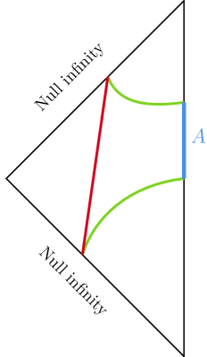
Figure 1: Geodesics connecting to $\partial A$ in the Poincare patch of $\text{AdS}_{3}$. The red line denotes one timelike geodesic and two green lines denote two spacelike geodesics. The blue line denotes a timelike interval $A$ on the conformal boundary.

The purpose of this paper is to confirm the predictions made in [1]. In the cAdS/dCFT correspondence, the general EE could be thought of a complete measure, which always receives a correction from the $T\bar{T}$ deformation. The spacelike and timelike entanglement entropies are different limits of the general entanglement entropy. As a consistent check, we will show that, the leading $T\bar{T}$ correction to the timelike EE exists in the finite size system, but vanishes in the finite temperature system. Utilizing the holographic method, we will show the physical reason why spacelike (timelike) EE only receives a correction in finite temperature (size) system.

The remainder of this paper is outlined as follows. In section 2, we show the leading correction of the general entanglement entropy of the $T\bar{T}$ deformed finite temperature $\text{CFT}_{2}$ and finite size $\text{CFT}_{2}$, respectively. In section 3, using RT formula, we show that the cutoff-AdS geodesic leads to a precise estimation of the general entanglement entropy in $T\bar{T}$ deformed CFT. Section 4 is devoted to our conclusions.

2 General entanglement entropy in $T\bar{T}$ deformed CFT

In this section, we calculate the leading corrections to the general EEof the $T\bar{T}$ deformed CFT living on the cylindrical manifold. After taking different limits, we derive the corrections to the spacelike EE and timelike EE respectively, for the finite temperature system and finite size system. For a $T\bar{T}$ deformed CFT on $\mathcal{M}$, the general EE of some subsystem $A\in\mathcal{M}$ is obtained by the definition of pseudoentropy. Substituting equation (1.2) into equation (1.6), one could obtain the leading correction to $S\left(A\right)$:

$$\delta S\left(A\right)=\lim_{n\rightarrow 1}\delta S_{n}\left(A\right),\quad\delta S_{n}\left(A\right)=\frac{n\mu}{1-n}\int_{\mathcal{M}}\left[\left\langle T\bar{T}\right\rangle_{\mathcal{M}}-\left\langle T\bar{T}\right\rangle_{\mathcal{M}_{n}}\right].$$ (2.10)

2.1 Finite temperature

Consider a $T\bar{T}$ deformed CFT at the inverse temperature $\beta$. This theory lives on a cylindrical manifold $\mathcal{M}_{1}$, which has a non-compact spatial direction $x\in\left(-\infty,\infty\right)$ and compact Euclidean time $\tau\in\left(0,\beta\right)$ with the periodicity $\tau\sim\tau+\beta$. It is well-known that the two-point correlation function in the finite temperature CFT is

$$\left\langle\mathcal{O}\left(w,\bar{w}\right)\mathcal{O}\left(0,0\right)\right\rangle = \left[\frac{\beta^{2}}{\pi^{2}}\sinh\left(\frac{\pi w}{\beta}\right)\sinh\left(\frac{\pi\bar{w}}{\beta}\right)\right]^{-2\Delta}$$ (2.11)

with the complex coordinate $w=x+i\tau$ and the scaling dimension $\Delta$. By the replica trick, the entanglement entropy of a single interval $A$, which has timelike width $\tau_{0}$ and spacelike width $x_{0}$, is related to the two-point function of the twist fields

$$\frac{Z_{\mathcal{M}_{n}}\left(A\right)}{Z_{\mathcal{M}_{1}}^{n}} = \Bigl{\langle}\Phi^{+}\left(0,0\right)\Phi^{-}\left(x_{0}+i\tau_{0},x_{0}-i\tau_{0}\right)\Bigr{\rangle}$$

$$= \left[\frac{\beta^{2}}{\pi^{2}\epsilon^{2}}\sinh\left(\frac{\pi\left(x_{0}+i\tau_{0}\right)}{\beta}\right)\sinh\left(\frac{\pi\left(x_{0}-i\tau_{0}\right)}{\beta}\right)\right]^{-2\Delta_{n}}$$

with the dimension$\Delta_{n}=\frac{c_{\text{AdS}}}{24}\left(n-\frac{1}{n}\right),$ the UV cutoff $\epsilon$ and the central charge $c_{\text{AdS}}$. Therefore, the entanglement entropy obtained by equation (1.6) is

$$S\left(A\right) = \frac{c_{\text{AdS}}}{6}\log\left[\frac{\beta^{2}}{\pi^{2}\epsilon^{2}}\sinh\left(\frac{\pi\left(x_{0}+i\tau_{0}\right)}{\beta}\right)\sinh\left(\frac{\pi\left(x_{0}-i\tau_{0}\right)}{\beta}\right)\right]$$ (2.12)

$$= \frac{c_{\text{AdS}}}{3}\log\left[\frac{\beta}{2\pi\epsilon}\sqrt{2\cosh\left(\frac{2\pi x_{0}}{\beta}\right)-2\cosh\left(\frac{2\pi i\tau_{0}}{\beta}\right)}\right].$$

Following Ref.[12], one could also calculate $\left\langle T\bar{T}\right\rangle_{\mathcal{M}_{1}}$ and $\left\langle T\bar{T}\right\rangle_{\mathcal{M}_{n}}$ in the finite temperature CFT:

$$\left\langle T\bar{T}\right\rangle_{\mathcal{M}_{1}}=\left(\frac{c_{\text{AdS}}}{12}\right)^{2}\left(\frac{2\pi^{2}}{\beta^{2}}\right)^{2},$$ (2.13)

$$\left\langle T\bar{T}\right\rangle_{\mathcal{M}_{n}}=\left(\frac{c_{\text{AdS}}}{12}\right)^{2}\left[\left(\frac{2\pi^{2}}{\beta^{2}}\right)^{2}-\frac{2\pi^{2}}{\beta^{2}}\left(n-1\right)\left(Q+\bar{Q}\right)+O\left(\left(n-1\right)^{2}\right)\right],$$ (2.14)

with the meromorphic function

$$Q\left(w\right)\coloneqq\frac{\sinh^{2}\left(\frac{\pi\left(x_{0}+i\tau_{0}\right)}{\beta}\right)}{\sinh^{2}\left(\frac{\pi\left(x_{0}+i\tau_{0}-w\right)}{\beta}\right)\sinh^{2}\left(\frac{\pi w}{\beta}\right)}.$$

Intuitively, $Q\left(w\right)$ has two poles ($w=0$ and $w=x_{0}+i\tau_{0}$) that correspond to the residues

$$\mathrm{Res}\left(Q,w=0\right) = \frac{2\pi}{\beta}\coth\left(\frac{\pi\left(x_{0}+i\tau_{0}\right)}{\beta}\right),$$

$$\mathrm{Res}\left(Q,w=x_{0}+i\tau_{0}\right) = -\frac{2\pi}{\beta}\coth\left(\frac{\pi\left(x_{0}+i\tau_{0}\right)}{\beta}\right).$$

The leading correction to $S\left(A\right)$ caused by $T\bar{T}$ deformation is thus

$$\delta S\left(A\right) = \lim_{n\rightarrow 1}\frac{n\mu}{1-n}\int_{\mathcal{M}_{1}}\left(\frac{c_{\text{AdS}}}{12}\right)^{2}\left[\frac{2\pi^{2}}{\beta^{2}}\left(n-1\right)\left(Q+\bar{Q}\right)+O\left(\left(n-1\right)^{2}\right)\right]$$ (2.15)

$$= -\mu\int_{\mathcal{M}_{1}}\left(\frac{c_{\text{AdS}}}{12}\right)^{2}\frac{2\pi^{2}}{\beta^{2}}\left(Q+\bar{Q}\right),$$ (2.16)

which, with the help of Cauchy’s residue theorem, could be simplified as

$$\delta S\left(A\right) = -2\pi\mu\int_{0}^{x_{0}}dx\,\left(\frac{c_{\text{AdS}}}{12}\right)^{2}\frac{2\pi^{2}}{\beta^{2}}\times\left[\mathrm{Res}\left(Q,0\right)+\mathrm{Res}\left(\bar{Q},0\right)\right],$$

$$= -\mu\frac{\pi^{4}c_{\text{AdS}}^{2}}{18\beta^{3}}x_{0}\left[\coth\left(\frac{\pi\left(x_{0}+i\tau_{0}\right)}{\beta}\right)+\coth\left(\frac{\pi\left(x_{0}-i\tau_{0}\right)}{\beta}\right)\right]$$

$$= -\mu\frac{\pi^{4}c_{\text{AdS}}^{2}}{9\beta^{3}}\frac{x_{0}\sinh\left(\frac{2\pi x_{0}}{\beta}\right)}{\cosh\left(\frac{2\pi x_{0}}{\beta}\right)-\cosh\left(\frac{2\pi i\tau_{0}}{\beta}\right)}.$$

Via an analytical continuation $\tau=it$, the entanglement entropy in the finite temperature system, to the leading order of $\mu$, reads

$$S^{(\mu)}\left(A\right)=\frac{c_{\text{AdS}}}{3}\log\left[\frac{\beta}{2\pi\epsilon}\sqrt{2\cosh\left(\frac{2\pi x_{0}}{\beta}\right)-2\cosh\left(\frac{2\pi t_{0}}{\beta}\right)}\right]-\mu\frac{\pi^{4}c_{\text{AdS}}^{2}}{9\beta^{3}}\frac{x_{0}\sinh\left(\frac{2\pi x_{0}}{\beta}\right)}{\cosh\left(\frac{2\pi x_{0}}{\beta}\right)-\cosh\left(\frac{2\pi t_{0}}{\beta}\right)}.$$ (2.17)

By choosing $\left(x_{0},t_{0}\right)=\left(0,T\right)$, one obtains the timelike entanglement entropy in the $T\bar{T}$ deformed finite temperature system

$$S_{T}^{\left(\mu\right)}=\frac{c_{\text{AdS}}}{3}\log\left[\frac{\beta}{\pi\epsilon}\sinh\left(\frac{\pi T}{\beta}\right)\right]+i\frac{c_{\text{AdS}}\pi}{6}.$$ (2.18)

Comparing the above result with the timelike EE in the original finite temperature system [15],

$$S_{T}=\frac{c_{\text{AdS}}}{3}\log\left[\frac{\beta}{\pi\epsilon}\sinh\left(\frac{\pi T}{\beta}\right)\right]+i\frac{c_{\text{AdS}}\pi}{6},$$ (2.19)

it is not surprising that, in the $T\bar{T}$ deformed finite temperature CFT₂, the timelike entanglement entropy does not receive a correction from the $T\bar{T}$ deformation. Moreover, it is worthwhile to note that the imaginary part of the timelike entanglement entropy originates from the complex logarithmic function. For the particular geometry we are considering, if one wishes to match the imaginary component, one should take the principle branch which has the correct magnitude [21]. Similarly, choosing $\left(x_{0},t_{0}\right)=\left(X,0\right)$, the spacelike entanglement entropy with $T\bar{T}$ correction is determined:

$$S_{X}^{\left(\mu\right)}\left(A\right)=\frac{c_{\text{AdS}}}{3}\log\left[\frac{\beta}{\pi\epsilon}\sinh\left(\frac{\pi X}{\beta}\right)\right]-\mu\frac{\pi^{4}c_{\text{AdS}}^{2}}{9\beta^{3}}X\coth\left(\frac{\pi X}{\beta}\right),$$ (2.20)

which exactly agrees with the result in [12].

2.2 Finite size

Now we focus on the $T\bar{T}$ deformed field theory living on a cylindrical manifold $\mathcal{M}_{2}$, which has a non-compact temporal direction $\tau\in\left(-\infty,\infty\right)$ and a compact spatial direction $x\in\left(0,L\right)$ with the periodicity $x\sim x+L$. It is important to notice that $\mathcal{M}_{1}$ and $\mathcal{M}_{2}$ have the same topology $R\times S^{1}$. Therefore, by setting $\beta=L$ and exchanging $x\leftrightarrow\tau$ in equations (2.12) and (2.15) and performing the analytical continuation $\tau=it$, one easily obtains the entanglement entropy in the finite size system

$$S^{(\mu)}\left(A\right)=\frac{c_{\text{AdS}}}{3}\log\left[\frac{L}{2\pi\epsilon}\sqrt{2\cos\frac{2\pi t_{0}}{L}-2\cos\frac{2\pi x_{0}}{L}}\right]+\mu\frac{\pi^{4}c_{\text{AdS}}^{2}}{9L^{3}}\frac{t_{0}\sin\left(\frac{2\pi t_{0}}{L}\right)}{\cos\left(\frac{2\pi t_{0}}{L}\right)-\cos\left(\frac{2\pi x_{0}}{L}\right)}.$$ (2.21)

Setting $\left(x_{0},t_{0}\right)=\left(0,T\right)$, the timelike entanglement entropy indeed receives a correction from the $T\bar{T}$ deformation

$$S_{T}^{(\mu)}\left(A\right)=\frac{c_{\text{AdS}}}{3}\log\left[\frac{L}{\pi\epsilon}\sin\left(\frac{\pi T}{L}\right)\right]-\mu\frac{\pi^{4}c_{\text{AdS}}^{2}}{9L^{3}}T\cot\left(\frac{\pi T}{L}\right)+i\frac{c_{\text{AdS}}\pi}{6}.$$ (2.22)

Meanwhile, as expected, the spacelike entanglement entropy does not receive a correction

$$S_{X}^{(\mu)}\left(A\right)=\frac{c_{\text{AdS}}}{3}\log\left[\frac{L}{\pi\epsilon}\sin\left(\frac{\pi X}{L}\right)\right].$$ (2.23)

	EE of a single interval	Leading $T\bar{T}$ correction
Finite size	Timelike: $S_{T}=\frac{c_{\text{AdS}}}{3}\log\left(\frac{L}{\pi\epsilon}\sin\left(\frac{\pi T}{L}\right)\right)+\frac{ic_{\text{AdS}}\pi}{6}$	$\delta S_{T}=-\mu\frac{\pi^{4}c_{\text{AdS}}^{2}}{9L^{3}}T\cot\left(\frac{\pi T}{L}\right)$
	Spacelike: $S_{X}=\frac{c_{\text{AdS}}}{3}\log\left(\frac{L}{\pi\epsilon}\sin\left(\frac{\pi X}{L}\right)\right)$	$\delta S_{X}=0$
Finite temperature	Timelike: $S_{T}=\frac{c_{\text{AdS}}}{3}\log\left(\frac{\beta}{\pi\epsilon}\sinh\frac{\pi T}{\epsilon}\right)+\frac{ic_{\text{AdS}}\pi}{6}$	$\delta S_{T}=0$
	Spacelike: $S_{X}=\frac{c_{\text{AdS}}}{3}\log\left(\frac{\beta}{\pi\epsilon}\sinh\frac{\pi X}{\epsilon}\right)$	$\delta S_{X}=-\mu\frac{\pi^{4}c_{\text{AdS}}^{2}}{9\beta^{3}}X\coth\left(\frac{\pi X}{\beta}\right)$

Table 2: The leading correction to the spacelike/timelike EE caused by the $T\bar{T}$ deformation in finite size/temperature system.

In the above field-theoretic results, the leading $T\bar{T}$ correction to the timelike EE exists in finite size systems but vanishes in finite temperature systems, while the leading $T\bar{T}$ correction to the spacelike EE exhibits the opposite behavior, as shown in Table 2, which is in perfect agreement with our prediction in [1]. Meanwhile, the leading $T\bar{T}$ correction to the general entanglement entropy always exists in both finite size systems and finite temperature systems. Therefore, the general entanglement entropy is the right measure to mark the deformations.

3 Gravity duals

It is illuminating to study the spacelike/timelike EE and its corresponding gravity dual in the context of cAdS/dCFT correspondence. In this section, we will demonstrate that the distance of the geodesic in the cutoff-AdS precisely matches the general entanglement entropy in the $T\bar{T}$ deformed $\text{CFT}_{2}$. We will only compute the geodesic length between two boundary points, which does not prove the existence of the geometric bulk dual of the general EE. However, the bulk dual of the timelike EE has been explicitly studied in [21].

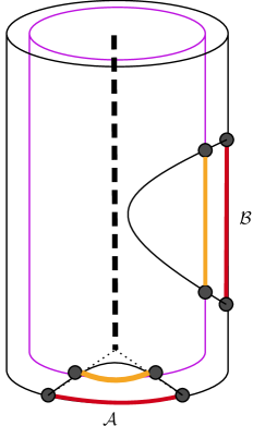
Figure 2: The figure illustrates a Euclidean cylindrical manifold with a black cylinder representing the original boundary and a violet cylinder representing the cut-off boundary. Two red lines denote an interval $\mathcal{A}$ in the compact direction and an interval $\mathcal{B}$ in the non-compact direction. Two orange lines indicate their corresponding intervals in the cut-off boundary.

Before that, we first provide a physical interpretation of our previous conjecture by introducing a Euclidean cylindrical manifold, as depicted in Figure 2, which features one compact and one non-compact direction. The compact direction is always described by a native parameter, either the inverse temperature $\beta$ in the finite temperature system or the total length $L$ in the finite size system. As a result, the interval $\mathcal{A}$ in the compact direction is independent of the cut-off boundary and the geodesic anchored on $\partial\mathcal{A}$ remains unchanged. The interval $\mathcal{A}$ in the compact direction is independent of the choice of the cut-off boundary, and the geodesic anchored on $\partial\mathcal{A}$ will not change. In contrast, the interval $\mathcal{B}$ in the non-compact direction will vary with the cut-off boundary, which leads to a change in the geodesic anchored on $\partial\mathcal{B}$. Therefore, in the finite temperature system, the temporal direction is compact and its timelike EE remains unaffected by the $T\bar{T}$ deformation; in the finite size system, the spatial direction is compact and its spacelike EE remains unchanged under the $T\bar{T}$ deformation.

3.1 BTZ black hole

Consider a BTZ black hole that is described by

$$ds^{2}=-\frac{r^{2}-r_{+}^{2}}{R_{\text{AdS}}^{2}}dt^{2}+\frac{R_{\text{AdS}}^{2}}{r^{2}-r_{+}^{2}}dr^{2}+\frac{r^{2}}{R_{\text{AdS}}^{2}}dx^{2},$$ (3.24)

where $r_{+}$ is the radius of event horizon, and $t$ is the compact temporal direction $t\sim t+i\beta$. It is well-known that the finite temperature $\text{CFT}_{2}$ is dual to a BTZ black hole with the same temperature

$$\beta^{-1}=\frac{r_{+}}{2\pi R_{\text{AdS}}^{2}},$$ (3.25)

In the cAdS/dCFT correspondence, the $T\bar{T}$ deformed CFT at finite temperature is dual to a BTZ black hole with the radial cutoff $r_{c}$,

$$r_{c}^{2}=\frac{6R_{\text{AdS}}^{4}}{\pi c_{\text{AdS}}\mu}.$$ (3.26)

Taking $r=r_{c}$ and multiplying a factor $R_{\text{AdS}}^{2}/(r_{c}^{2}-r_{+}^{2})$ in the BTZ black hole metric, the metric of the cutoff boundary, where the $T\bar{T}$ deformed CFT lives, reads

$$ds^{2}=-dt^{2}+\frac{dx^{2}}{1-r_{+}^{2}/r_{c}^{2}}.$$ (3.27)

Notice that the timelike interval on the boundary keeps invariant, because the compact temporal direction should be physical. This is the reason that the timelike EE does not receive a correction from the $T\bar{T}$ deformation. To see this, for an interval $A$, with the timelike width $t_{0}$ and the spacelike width $x_{0}$, in the $T\bar{T}$ deformed CFT, we calculate the general entanglement entropy with the RT formula. Performing the following coordinates transformation,

$$u = \sqrt{1-\frac{r_{+}^{2}}{r^{2}}}\cosh\left(\frac{r_{+}t}{R_{\text{AdS}}^{2}}\right)\exp\left(\frac{r_{+}x}{R_{\text{AdS}}^{2}}\right),$$

$$v = \sqrt{1-\frac{r_{+}^{2}}{r^{2}}}\sinh\left(\frac{r_{+}t}{R_{\text{AdS}}^{2}}\right)\exp\left(\frac{r_{+}x}{R_{\text{AdS}}^{2}}\right),$$ (3.28)

$$z = \frac{r_{+}}{r}\exp\left(\frac{r_{+}x}{R_{\text{AdS}}^{2}}\right),$$

the metric (3.24) becomes

$$ds^{2}=\frac{R_{\text{AdS}}^{2}}{z^{2}}\left(du^{2}-dv^{2}+dz^{2}\right).$$ (3.29)

Two boundary points $\partial A=\left\{\left(u_{1},v_{1},z_{1}\right),\left(u_{2},v_{2},z_{2}\right)\right\}$ could be written as

$$\begin{cases}u_{1}=\sqrt{1-\frac{r_{+}^{2}}{r_{c}^{2}}},&u_{2}=\sqrt{1-\frac{r_{+}^{2}}{r_{c}^{2}}}\cosh\left(\frac{r_{+}t_{0}}{R_{\text{AdS}}^{2}}\right)\exp\left(\frac{r_{+}x_{0}}{R_{\text{AdS}}^{2}}\sqrt{1-\frac{r_{+}^{2}}{r_{c}^{2}}}\right),\\ v_{1}=0,&v_{2}=\sqrt{1-\frac{r_{+}^{2}}{r_{c}^{2}}}\sinh\left(\frac{r_{+}t_{0}}{R_{\text{AdS}}^{2}}\right)\exp\left(\frac{r_{+}x_{0}}{R_{\text{AdS}}^{2}}\sqrt{1-\frac{r_{+}^{2}}{r_{c}^{2}}}\right),\\ z_{1}=\frac{r_{+}}{r_{c}},&z_{2}=\frac{r_{+}}{r_{c}}\exp\left(\frac{r_{+}x_{0}}{R_{\text{AdS}}^{2}}\sqrt{1-r_{+}^{2}/r_{c}^{2}}\right).\end{cases}$$ (3.30)

Therefore, one can determine the length of the geodesic $\gamma_{A}$ to be

$$L_{\gamma_{A}} = R_{\text{AdS}}\,\mathrm{arcosh}\left[1+\frac{\left(u_{2}-u_{1}\right)^{2}-\left(v_{2}-v_{1}\right)^{2}+\left(z_{2}-z_{1}\right)^{2}}{2z_{1}z_{2}}\right]$$ (3.31)

$$= R_{\text{AdS}}\,\mathrm{arcosh}\left[\frac{\left(r_{+}^{2}/r_{c}^{2}-1\right)\cosh\left(\frac{r_{+}t_{0}}{R_{\text{AdS}}^{2}}\right)+\cosh\left(\frac{r_{+}x_{0}}{R_{\text{AdS}}^{2}}\sqrt{1-r_{+}^{2}/r_{c}^{2}}\right)}{r_{+}^{2}/r_{c}^{2}}\right]$$

$$= 2R_{\text{AdS}}\log\left[\frac{r_{c}}{r_{+}}\sqrt{2\cosh\left(\frac{r_{+}x_{0}}{R_{\text{AdS}}^{2}}\right)-2\cosh\left(\frac{r_{+}t_{0}}{R_{\text{AdS}}^{2}}\right)}\right]-\frac{r_{+}^{2}}{r_{c}^{2}}\frac{\frac{r_{+}x_{0}}{2R_{\text{AdS}}}\sinh(\frac{r_{+}x_{0}}{R_{\text{AdS}}^{2}})}{\cosh(\frac{r_{+}x_{0}}{R_{\text{AdS}}^{2}})-\cosh(\frac{r_{+}t_{0}}{R_{\text{AdS}}^{2}})}$$

$$+\frac{r_{+}^{2}}{r_{c}^{2}}\frac{R_{\text{AdS}}\,\cosh(\frac{r_{+}t_{0}}{R_{\text{AdS}}^{2}})}{\cosh(\frac{r_{+}x_{0}}{R_{\text{AdS}}^{2}})-\cosh(\frac{r_{+}t_{0}}{R_{\text{AdS}}^{2}})}+O\left(\frac{r_{+}^{3}}{r_{c}^{3}}\right).$$

Notice that the first term in the last line should not be thought of a leading correction caused by $T\bar{T}$ flow. To see this point, replacing the metric of the cutoff boundary with $ds^{2}=-dt^{2}+dx^{2}$, one can compute the length of the geodesic $\gamma_{A}$:

$$L_{\gamma_{A}} = R_{\text{AdS}}\,\mathrm{arcosh}\left[\frac{\left(r_{+}^{2}/r_{c}^{2}-1\right)\cosh\left(\frac{r_{+}t_{0}}{R_{\text{AdS}}^{2}}\right)+\cosh\left(\frac{r_{+}x_{0}}{R_{\text{AdS}}^{2}}\right)}{r_{+}^{2}/r_{c}^{2}}\right]$$ (3.32)

$$= 2R_{\text{AdS}}\log\left[\frac{r_{c}}{r_{+}}\sqrt{2\cosh\left(\frac{r_{+}x_{0}}{R_{\text{AdS}}^{2}}\right)-2\cosh\left(\frac{r_{+}t_{0}}{R_{\text{AdS}}^{2}}\right)}\right]$$

$$+\frac{r_{+}^{2}}{r_{c}^{2}}\frac{R_{\text{AdS}}\cosh(\frac{r_{+}t_{0}}{R_{\text{AdS}}^{2}})}{\cosh(\frac{r_{+}x_{0}}{R_{\text{AdS}}^{2}})-\cosh(\frac{r_{+}t_{0}}{R_{\text{AdS}}^{2}})}+O\left(\frac{r_{+}^{3}}{r_{c}^{3}}\right).$$

Therefore, utilizing equations (3.25) and (3.26) and identifying $\epsilon^{2}=\pi c_{\text{AdS}}\mu/6$, the right estimation of the general entanglement entropy corrected by $T\bar{T}$ deformation is

$$\frac{L_{\gamma_{A}}}{4G_{N}}\sim\frac{R_{\text{AdS}}}{2G_{N}}\log\left[\frac{\beta}{2\pi\epsilon}\sqrt{2\cosh\left(\frac{2\pi x_{0}}{\beta}\right)-2\cosh\left(\frac{2\pi t_{0}}{\beta}\right)}\right]-\frac{R_{\text{AdS}}}{2G_{N}}\frac{\pi^{3}c_{\text{AdS}}\mu}{3\beta^{2}}\frac{\frac{\pi x_{0}}{\beta}\sinh(\frac{2\pi x_{0}}{\beta})}{\cosh(\frac{2\pi x_{0}}{\beta})-\cosh(\frac{2\pi t_{0}}{\beta})},$$ (3.33)

that is

$$S_{A}^{(\mu)}=\frac{c_{\text{AdS}}}{3}\log\left[\frac{\beta}{2\pi\epsilon}\sqrt{2\cosh\left(\frac{2\pi x_{0}}{\beta}\right)-2\cosh\left(\frac{2\pi t_{0}}{\beta}\right)}\right]-\mu\frac{\pi^{4}c_{\text{AdS}}^{2}}{9\beta^{3}}\frac{x_{0}\sinh(\frac{2\pi x_{0}}{\beta})}{\cosh(\frac{2\pi x_{0}}{\beta})-\cosh(\frac{2\pi t_{0}}{\beta})}$$ (3.34)

This precisely matches the field theoretic result (2.17).

3.2 Global $\text{AdS}_{3}$

Consider the finite size $\text{CFT}_{2}$ at zero temperature that is dual to the global $\text{AdS}_{3}$. The metric of the global $\text{AdS}_{3}$ is given by

$$ds^{2}=R_{\text{AdS}}^{2}\left(-\cosh^{2}\rho\,d\theta^{2}+d\rho^{2}+\sinh^{2}\rho\,d\phi^{2}\right),$$ (3.35)

where $\phi$ is the compact spatial direction $\phi\sim\phi+2\pi$. In the cAdS/dCFT correspondence, the $T\bar{T}$ deformed CFT lives at the radial cutoff $\rho_{c}$,

$$\cosh^{2}\rho_{c}=\frac{3L^{2}}{2\mu\pi^{3}c_{\text{AdS}}},$$ (3.36)

where the total length of the boundary circle is $L$, and the metric of the cutoff boundary reads

$$ds^{2}=-\coth^{2}\rho_{c}\,d\theta^{2}+d\phi^{2}.$$ (3.37)

Intriguingly, the timelike interval in the boundary is indeed changed by $T\bar{T}$ deformation, which means that timelike EE in the finite size system will be corrected by $T\bar{T}$ deformation. By choosing an interval $A$ with the timelike width $t_{0}=\frac{L\theta_{0}}{2\pi}$ and the spacelike width $x_{0}=\frac{L\phi_{0}}{2\pi}$, and performing the following coordinates transformation,

$$u = \tanh\rho\cos\left(\theta\right)\exp\left(i\phi\right),$$

$$v = \tanh\rho\sin\left(\theta\right)\exp\left(i\phi\right),$$ (3.38)

$$z = \frac{1}{\cosh\rho}\exp\left(i\phi\right),$$

the metric (3.35) becomes

$$ds^{2}=\frac{R_{\text{AdS}}^{2}}{z^{2}}\left(du^{2}+dv^{2}+dz^{2}\right).$$ (3.39)

The two boundary points $\partial A=\left\{\left(u_{1},v_{1},z_{1}\right),\left(u_{2},v_{2},z_{2}\right)\right\}$ could be written as

$$\begin{cases}u_{1}=\tanh\rho_{c},&u_{2}=\tanh\rho_{c}\cos\left(\frac{2\pi x_{0}}{L}\right)\exp\left(i\frac{2\pi t_{0}}{L}\tanh\rho_{c}\right),\\ v_{1}=0,&v_{2}=\tanh\rho_{c}\sin\left(\frac{2\pi x_{0}}{L}\right)\exp\left(i\frac{2\pi t_{0}}{L}\tanh\rho_{c}\right),\\ z_{1}=\frac{1}{\cosh\rho_{c}},&z_{2}=\frac{1}{\cosh\rho_{c}}\exp\left(i\frac{2\pi t_{0}}{L}\tanh\rho_{c}\right),\end{cases}$$ (3.40)

and the distance of the geodesic $\gamma_{A}$, anchored on $\partial A$, could be captured by

$$L_{\gamma_{A}} = R_{\text{AdS}}\,\mathrm{arcosh}\left[\frac{\cos\left(\frac{2\pi t_{0}}{L}\tanh\rho_{c}\right)+\left(\cosh^{-2}\rho_{c}-1\right)\cos\left(\frac{2\pi x_{0}}{L}\right)}{\cosh^{-2}\rho_{c}}\right]$$ (3.41)

$$= 2R_{\text{AdS}}\log\left[\cosh\rho_{c}\sqrt{2\cos\left(\frac{2\pi t_{0}}{L}\right)-2\cos\left(\frac{2\pi x_{0}}{L}\right)}\right]+\frac{\frac{R_{\text{AdS}}}{\cosh^{2}\rho_{c}}\frac{\pi t_{0}}{L}\sin\left(\frac{2\pi t_{0}}{L}\right)}{\cos\left(\frac{2\pi t_{0}}{L}\right)-\cos\left(\frac{2\pi x_{0}}{L}\right)}$$

$$+\frac{R_{\text{AdS}}}{\cosh^{2}\rho_{c}}\frac{\cos\left(\frac{2\pi t_{0}}{L}\right)}{\cos\left(\frac{2\pi t_{0}}{L}\right)-\cos\left(\frac{2\pi x_{0}}{L}\right)}+O\left(\frac{1}{\cosh^{3}\rho_{c}}\right)$$

$$\sim 2R_{\text{AdS}}\log\left[\cosh\rho_{c}\sqrt{2\cos\left(\frac{2\pi t_{0}}{L}\right)-2\cos\left(\frac{2\pi x_{0}}{L}\right)}\right]+\frac{\frac{R_{\text{AdS}}}{\cosh^{2}\rho_{c}}\frac{\pi t_{0}}{L}\sin\left(\frac{2\pi t_{0}}{L}\right)}{\cos\left(\frac{2\pi t_{0}}{L}\right)-\cos\left(\frac{2\pi x_{0}}{L}\right)}.$$ (3.42)

Substituting equation (3.36) into equation (3.42), and identifying $\epsilon^{2}=\pi c\mu/6$, one obtains

$$L_{\gamma_{A}} \sim 2R_{\text{AdS}}\log\left[\frac{L}{2\pi\epsilon}\sqrt{2\cos\left(\frac{2\pi t_{0}}{L}\right)-2\cos\left(\frac{2\pi x_{0}}{L}\right)}\right]+\frac{2\mu\pi^{4}c_{\text{AdS}}}{3L^{3}}\frac{R_{\text{AdS}}t_{0}\sin\left(\frac{2\pi t_{0}}{L}\right)}{\cos\left(\frac{2\pi t_{0}}{L}\right)-\cos\left(\frac{2\pi x_{0}}{L}\right)}.$$ (3.43)

With the RT formula, one finds the following estimation of the general entanglement entropy:

$$S_{A}^{(\mu)} = \frac{c_{\text{AdS}}}{3}\log\left[\frac{L}{2\pi\epsilon}\sqrt{2\cos\left(\frac{2\pi t_{0}}{L}\right)-2\cos\left(\frac{2\pi x_{0}}{L}\right)}\right]+\frac{\mu\pi^{4}c_{\text{AdS}}^{2}}{9L^{3}}\frac{t_{0}\sin\left(\frac{2\pi t_{0}}{L}\right)}{\cos\left(\frac{2\pi t_{0}}{L}\right)-\cos\left(\frac{2\pi x_{0}}{L}\right)},$$ (3.44)

which is a perfect match with the field theoretic result (2.22).

4 Conclusions

The $T\bar{T}$ deformation has been widely studied in recent years, due to its integrability in 2$d$ CFTs and its applications in holography. In a previous work, we had amazingly found that the usual spacelike entanglement entropy alone is not sufficient to fully mark the $T\bar{T}$ deformation and that a timelike entanglement entropy must be introduced. The conventional spacelike entanglement entropy fails to fully capture the entangling properties, as it remains unchanged between the undeformed finite-size CFT and the $T\bar{T}$ deformed one. In this paper, we show that, complementarily, the timelike entanglement entropy could distinguish the undeformed finite-size CFT and the $T\bar{T}$ deformed one. In the context of cAdS/dCFT correspondence, we affirm the indispensability of the timelike entanglement entropy, as it proves crucial in differentiating between the undeformed CFT and the $T\bar{T}$ deformed CFT. Our main results have been shown in Table 2.

In this paper, our findings heavily rely on the AdS/CFT correspondence. It is equally crucial to investigate the timelike entanglement entropy within the framework of the dS/CFT correspondence. Moreover, the physical interpretation of the timelike entanglement entropy remains obscure, making explicit studies on this topic of utmost importance. Consequently, the timelike entanglement entropy may hold significant potential in enhancing our comprehension of black hole information and the emergence of spacetime geometry from entanglement.

Acknowledgements This work is supported in part by NSFC (Grant No. 12275183, 12275184, 12105191 and 11875196). HW is supported by the International Visiting Program for Excellent Young Scholars of Sichuan University.