Iterated Filters for Nonlinear Transition Models

Abstract

A new class of iterated linearization-based nonlinear filters, dubbed dynamically iterated filters, is presented. Contrary to regular iterated filters such as the iterated extended Kalman filter (IEKF), iterated unscented Kalman filter (IUKF) and iterated posterior linearization filter (IPLF), dynamically iterated filters also take nonlinearities in the transition model into account. The general filtering algorithm is shown to essentially be a (locally over one time step) iterated Rauch-Tung-Striebel smoother. Three distinct versions of the dynamically iterated filters are especially investigated: analogues to the IEKF, IUKF and IPLF. The developed algorithms are evaluated on 25 different noise configurations of a tracking problem with a nonlinear transition model and linear measurement model, a scenario where conventional iterated filters are not useful. Even in this “simple” scenario, the dynamically iterated filters are shown to have superior root mean-squared error performance as compared with their respective baselines, the EKF and UKF. Particularly, even though the EKF diverges in 22 out of 25 configurations, the dynamically iterated EKF remains stable in 20 out of 25 scenarios, only diverging under high noise.

I Introduction

State estimation in dynamical systems is a universal problem occurring in the fields of engineering, robotics, economics, etc. State estimation requires a system model describing the dynamical evolution of the system and a measurement model relating the measured quantities to the state of the system. If the model is affine with additive Gaussian noise, the most well-known state estimation algorithm is the analytically tractable Kalman filter, which is the optimal estimator in the mean-squared error (mse) sense [1].

In many practical problems, a nonlinear system model is necessary to accurately describe the system. This means that the state estimation problem is no longer analytically tractable and approximate inference techniques must be used. Approximate inference in state-space models is a well-studied field in signal processing, machine learning, etc. Here, we shall focus on linearization-based approximate inference techniques. These inference techniques linearize the nonlinear model locally (in each time instance) and then employ the Kalman filter. Analytical linearization leads to the extended Kalman filter (ekf), while sigma-point filters, such as the unscented Kalman filter (ukf) and the cubature Kalman filter (ckf), can be thought of as statistical linearization filters [2, 1, 3].

General (Gaussian) state-space models, in the form of a transition model and a measurement model, may equivalently be probabilistically interpreted as a transition density and a measurement density. Under this interpretation, the linearization-based approximate inference techniques can be thought of as approximating the transition and measurement densities, e.g.,

$$\mathbf{x}_{k+1} =\mathbf{f}(\mathbf{x}_{k},\mathbf{w}_{k}) \mathchoice{\leavevmode\hbox to20pt{\vbox to1pt{\text{[drawing]}}}}{\leavevmode\hbox to20pt{\vbox to1pt{\text{[drawing]}}}}{\leavevmode\hbox to14pt{\vbox to1pt{\text{[drawing]}}}}{\leavevmode\hbox to10pt{\vbox to1pt{\text{[drawing]}}}}p(\mathbf{x}_{k+1}|\mathbf{x}_{k}) \overset{a}{\approx}q(\mathbf{x}_{k+1}|\mathbf{x}_{k})$$

$$\mathbf{y}_{k} =\mathbf{h}(\mathbf{x}_{k},\mathbf{e}_{k}) \qquad p(\mathbf{y}_{k}|\mathbf{x}_{k}) \overset{a}{\approx}q(\mathbf{y}_{k}|\mathbf{x}_{k}),$$

where $p(\mathbf{x}_{k+1}|\mathbf{x}_{k})$ and $p(\mathbf{y}_{k}|\mathbf{x}_{k})$ are the transition and measurement density and $q(\mathbf{x}_{k+1}|\mathbf{x}_{k})$ and $q(\mathbf{y}_{k}|\mathbf{x}_{k})$ the corresponding approximations. Particularly, the linearization-based filters assume affine Gaussian densities for $q(\mathbf{x}_{k+1}|\mathbf{x}_{k})$ and $q(\mathbf{y}_{k}|\mathbf{x}_{k})$ and the Kalman filter is then applied to this “auxiliary” model. The quality of the auxiliary model, and in extension the estimation performance of linearization-based filters, is thus highly dependent on the point (distribution in the statistical case) about which the models are linearized. Typically, the linearization point (distribution) is chosen to be the mean (distribution) of the current state estimate. However, a large error in the state estimate can lead to significant linearization errors that may cause even larger estimation errors in the next time step. This may, in the worst case, cause the filter to diverge. To alleviate such issues, several variants of iterated filters have been developed, such as the iterated extended Kalman filter (iekf), the iterated unscented Kalman filter (iukf) and the iterated posterior linearization filter (iplf) [4, 5, 6, 7, 8]. These filters essentially iterate the measurement update, where each iteration the measurement model is re-linearized with the “latest” iterate. The research efforts within the field of iterated filters have particularly focused on finding a better linearization point for the measurement model, which is motivated by the fact that nonlinearities in the measurement model (likelihood) affect the resulting state estimate to a greater extent than nonlinearities in the transition model (prior). Nevertheless, these methods are for instance not useful in the case of a nonlinear transition model but linear measurement model.

In this paper, we seek to fill this gap by developing a class of iterated filters encompassing both the transition model and the measurement model in the iterative process, which we dub dynamically iterated filters. Note that a dynamically iterated filter based on posterior linearization was first derived in [9] for models with non-additive state transition noise. Further, the L-scan iplf in [10] is somewhat similar to the dynamical iplf developed here, but requires access to past observations and is thus not strictly a filter. In this paper, we particularly focus on additive noise models and treat both analytical as well as statistical linearization in a common framework. The algorithms developed here are essentially dynamically iterated analogues of the iekf, iukf and iplf, as well as other iterated sigma-point filters and does thus not require access to past observations. These new iterative algorithms encompass both the transition model as well as the measurement model. Thereby, the proposed algorithms constitute a generalization of conventional iterated filters. To illustrate the benefits of the proposed algorithms, it is empirically shown that iterating over the transition linearization improves the estimation performance even in the case of a linear measurement model. Thus, the contributions are twofold:

• A detailed derivation of dynamically iterated filters

• An extensive numerical evaluation of the developed algorithms as compared to standard nonlinear filters

The paper is organized as follows. In Section II, analytical and statistical linearization as well as the (affine) Kalman smoother equations are restated for completeness. In Section III, the state estimation problem is formulated in terms of approximate transition and measurement densities. Section IV derives the dynamically iterated filters and connects the final solution to iterated (affine) smoothers. Lastly, Section V provides a numerical example of the developed algorithm in a tracking scenario where conventional iterated filters are not useful.

II Background

For clarity, we here present analytical and statistical linearization in a common framework, as well as restate the well-known Kalman smoother equations.

II-A (Affine) Kalman Smoother

The well-known Kalman filter and Rauch-Tung-Striebel (rts) smoother equations are repeated here for clarity in terms of a time update, measurement update, and a smoothing step. These can for instance be found in [11]. Assume an affine state-space model with additive Gaussian noise, such as

$$\mathbf{x}_{k+1} =\mathbf{A}_{\mathbf{f}}\mathbf{x}_{k}+\mathbf{b}_{\mathbf{f}}+\tilde{\mathbf{w}}_{k}$$ (1a)

$$\mathbf{y}_{k} =\mathbf{A}_{\mathbf{h}}\mathbf{x}_{k}+\mathbf{b}_{\mathbf{h}}+\tilde{\mathbf{e}}_{k}.$$ (1b)

Here, $\tilde{\mathbf{w}}_{k}\sim\mathcal{N}(\tilde{\mathbf{w}}_{k};\mathbf{0},\mathbf{Q}\!+\!\bm{\Omega}_{\mathbf{f}})$ and $\tilde{\mathbf{e}}_{k}\sim\mathcal{N}(\tilde{\mathbf{e}}_{k};\mathbf{0},\mathbf{R}\!+\!\bm{\Omega}_{\mathbf{h}})$ are assumed to be mutually independent. Note that usually, $\bm{\Omega}_{\mathbf{f}}=\bm{\Omega}_{\mathbf{h}}=\mathbf{0}$. For this model, the (affine) Kalman smoother update equations are given by Algorithm 1.

Algorithm 1 (Affine) Kalman smoother

1. Time update

   $$\hat{\mathbf{x}}_{k+1|k} =\mathbf{A}_{\mathbf{f}}\hat{\mathbf{x}}_{k|k}+\mathbf{b}_{\mathbf{f}}$$ (2a)

   $$\mathbf{P}_{k+1|k} =\mathbf{A}_{\mathbf{f}}\mathbf{P}_{k|k}\mathbf{A}_{\mathbf{f}}^{\top}+\mathbf{Q}+\bm{\Omega}_{\mathbf{f}}.$$ (2b)

2. Measurement update

   $$\hat{\mathbf{x}}_{k|k} =\hat{\mathbf{x}}_{k|k-1}+\mathbf{K}_{k}(\mathbf{y}_{k}-\mathbf{A}_{\mathbf{h}}\hat{\mathbf{x}}_{k|k-1}-\mathbf{b}_{\mathbf{h}})$$ (3a)

   $$\mathbf{P}_{k|k} =\mathbf{P}_{k|k-1}-\mathbf{K}_{k}\mathbf{A}_{\mathbf{h}}\mathbf{P}_{k|k-1}$$ (3b)

   $$\mathbf{K}_{k} \triangleq\mathbf{P}_{k|k-1}\mathbf{A}_{\mathbf{h}}^{\top}(\mathbf{A}_{\mathbf{h}}\mathbf{P}_{k|k-1}\mathbf{A}_{\mathbf{h}}^{\top}+\mathbf{R}+\bm{\Omega}_{\mathbf{h}})^{-1}.$$ (3c)

3. Smoothing step

   $$\hat{\mathbf{x}}^{s}_{k|K} =\hat{\mathbf{x}}_{k|k}+\mathbf{G}_{k}(\hat{\mathbf{x}}^{s}_{k+1|K}-\hat{\mathbf{x}}_{k+1|k})$$ (4a)

   $$\mathbf{P}^{s}_{k|K} =\mathbf{P}_{k|k}+\mathbf{G}_{k}(\mathbf{P}^{s}_{k+1|K}-$$

   $$\quad~{}\mathbf{A}_{\mathbf{f}}\mathbf{P}_{k|k}\mathbf{A}_{\mathbf{f}}^{\top}-\mathbf{Q}-\bm{\Omega}_{\mathbf{f}})\mathbf{G}_{k}^{\top}$$ (4b)

   $$\mathbf{G}_{k} \triangleq\mathbf{P}_{k|k}\mathbf{A}_{\mathbf{f}}^{\top}(\mathbf{A}_{\mathbf{f}}\mathbf{P}_{k|k}\mathbf{A}_{\mathbf{f}}^{\top}+\mathbf{Q}+\bm{\Omega}_{\mathbf{f}})^{-1}$$ (4c)

II-B Analytical and Statistical Linearization

Given a nonlinear model

$$\mathbf{z}=\mathbf{g}(\mathbf{x}),$$

we wish to find an affine representation

$$\mathbf{g}(\mathbf{x})\approx\mathbf{A}\mathbf{x}+\mathbf{b}+\eta,$$ (5)

with $\eta\sim\mathcal{N}(\eta;\mathbf{0},\bm{\Omega})$. In this affine representation, there are three free parameters: $\mathbf{A},\mathbf{b}$ and $\bm{\Omega}$. Analytical linearization through first-order Taylor expansion selects the parameters as

$$\mathbf{A}=\frac{d}{d\mathbf{x}}\mathbf{g}(\mathbf{x})|_{\mathbf{x}=\bar{\mathbf{x}}},\quad\mathbf{b}=\mathbf{g}(\mathbf{x})|_{\mathbf{x}=\bar{\mathbf{x}}}-\mathbf{A}\bar{\mathbf{x}},\quad\bm{\Omega}=\mathbf{0},$$ (6)

where $\bar{\mathbf{x}}$ is the point about which the function $\mathbf{g}(\mathbf{x})$ is linearized. Note that $\bm{\Omega}=\mathbf{0}$ essentially implies that the linearization is assumed to be error free.

Statistical linearization instead linearizes w.r.t. a distribution $p(\mathbf{x})$. Assuming that such a distribution $p(\mathbf{x})=\mathcal{N}(\mathbf{x};\hat{\mathbf{x}},\mathbf{P})$ is given, statistical linearization selects the affine parameters as

$$\mathbf{A} =\Psi^{\top}\mathbf{P}^{-1}$$ (7a)

$$\mathbf{b} =\bar{\mathbf{z}}-\mathbf{A}\hat{\mathbf{x}}$$ (7b)

$$\bm{\Omega} =\Phi-\mathbf{A}\mathbf{P}\mathbf{A}^{\top}$$ (7c)

$$\bar{\mathbf{z}} =\mathbb{E}[\mathbf{g}(\mathbf{x})]$$ (7d)

$$\Psi =\mathbb{E}[(\mathbf{x}-\hat{\mathbf{x}})(\mathbf{g}(\mathbf{x})-\bar{\mathbf{z}})^{\top}]$$ (7e)

$$\Phi =\mathbb{E}[(\mathbf{g}(\mathbf{x})-\bar{\mathbf{z}})(\mathbf{g}(\mathbf{x})-\bar{\mathbf{z}})^{\top}],$$ (7f)

where the expectations are taken w.r.t. $p(\mathbf{x})$. The major difference from analytical linearization is that ${\bm{\Omega}\neq 0}$, implying that the error in the linearization is captured.

III Problem Formulation

To set the stage for the algorithm development, the general state estimation problem is described here with a probabilistic viewpoint. To that end, consider a discrete-time state-space model (omitting a possible input $\mathbf{u}_{k}$ for notational brevity) given by

$$\mathbf{x}_{k+1} =\mathbf{f}(\mathbf{x}_{k})+\mathbf{w}_{k}$$ (8a)

$$\mathbf{y}_{k} =\mathbf{h}(\mathbf{x}_{k})+\mathbf{e}_{k}$$ (8b)

$$p(\mathbf{w}_{k}) =\mathcal{N}(\mathbf{w}_{k};\mathbf{0},\mathbf{Q}),\quad p(\mathbf{e}_{k})=\mathcal{N}(\mathbf{e}_{k};\mathbf{0},\mathbf{R}).$$ (8c)

Here, $\mathbf{x}_{k},~{}\mathbf{y}_{k},~{}\mathbf{w}_{k}$ and $\mathbf{e}_{k}$ denote the state, the measurement, the process noise and the measurement noise at time $k$, respectively. It is further assumed that $\mathbf{x}_{k}\in\mathcal{X},\forall k$ and that $\mathbf{w}_{k}$ and $\mathbf{e}_{k}$ are mutually independent. Note that 8a and 8b can equivalently be written as a transition density and a measurement density as

$$p(\mathbf{x}_{k+1}|\mathbf{x}_{k}) =\mathcal{N}(\mathbf{x}_{k+1};\mathbf{f}(\mathbf{x}_{k}),\mathbf{Q})$$ (9a)

$$p(\mathbf{y}_{k}|\mathbf{x}_{k}) =\mathcal{N}(\mathbf{y}_{k};\mathbf{h}(\mathbf{x}_{k}),\mathbf{R}).$$ (9b)

Further, the initial state distribution is assumed to be given by

$$p(\mathbf{x}_{0})=\mathcal{N}(\mathbf{x}_{0};\hat{\mathbf{x}}_{0|0},\mathbf{P}_{0|0}).$$ (10)

Given the transition and measurement densities and a sequence of measurements $\mathbf{y}_{1:k}=\begin{bmatrix}\mathbf{y}_{1}^{\top}&\dots&\mathbf{y}_{k}^{\top}\end{bmatrix}^{\top}$, the state estimation problem consists of computing the posterior of the state sequence (trajectory), i.e., computing

$$p(\mathbf{x}_{0:k}|\mathbf{y}_{1:k})=\frac{1}{\mathbf{Z}_{1:k}}p(\mathbf{x}_{0})\prod_{i=1}^{k}p(\mathbf{y}_{i}|\mathbf{x}_{i})p(\mathbf{x}_{i}|\mathbf{x}_{i-1}),$$ (11)

where

$$\mathbf{Z}_{1:k}=\int_{\mathcal{X}}p(\mathbf{x}_{0})\prod_{i=1}^{k}p(\mathbf{y}_{i}|\mathbf{x}_{i})p(\mathbf{x}_{i}|\mathbf{x}_{i-1})d\mathbf{x}_{0}\cdots d\mathbf{x}_{k},$$

is the marginal likelihood of $\mathbf{y}_{1:k}$. The posterior (11) is commonly referred to as the joint smoothing distribution which, in the case of linear $\mathbf{f}$ and $\mathbf{h}$, can be analytically found through the Kalman smoother, e.g., the rts smoother [11].

In the setting considered here, i.e., in filtering applications, the densities of interest are rather the marginal posteriors

$$p(\mathbf{x}_{k}|\mathbf{y}_{1:k})=\frac{p(\mathbf{y}_{k}|\mathbf{x}_{k})\!\int_{\mathcal{X}}\!p(\mathbf{x}_{k}|\mathbf{x}_{k-1})p(\mathbf{x}_{k-1}|\mathbf{y}_{1:k-1})d\mathbf{x}_{k-1}}{\mathbf{Z}_{k}},$$ (12)

for all times $k$, where

$$\mathbf{Z}_{k}=\int_{\mathcal{X}}p(\mathbf{y}_{k}|\mathbf{x}_{k})p(\mathbf{x}_{k}|\mathbf{x}_{k-1})p(\mathbf{x}_{k-1}|\mathbf{y}_{1:k-1})d\mathbf{x}_{k-1}d\mathbf{x}_{k}.$$

Again, in the case of linear $\mathbf{f}$ and $\mathbf{h}$, the (analytical) solution is given by the Kalman filter [1].

In the general case, the marginal posteriors can not be computed analytically. Inspecting 12, there are two integrals that require attention. We turn first to the Chapman-Kolmogorov equation

$$p(\mathbf{x}_{k}|\mathbf{y}_{1:k-1})=\int_{\mathcal{X}}p(\mathbf{x}_{k}|\mathbf{x}_{k-1})p(\mathbf{x}_{k-1}|\mathbf{y}_{1:k-1})d\mathbf{x}_{k-1}.$$ (13)

Assuming that $p(\mathbf{x}_{k-1}|\mathbf{y}_{1:k-1})$ is Gaussian, 13 has a closed form solution given by 2, if $p(\mathbf{x}_{k}|\mathbf{x}_{k-1})$ is Gaussian and 8a is affine. Therefore, as 9a is Gaussian, we seek an affine approximation of the transition function $\mathbf{f}$ as

$$\mathbf{f}(\mathbf{x}_{k-1})\approx\mathbf{A}_{\mathbf{f}}\mathbf{x}_{k-1}+\mathbf{b}_{\mathbf{f}}+\eta_{\mathbf{f}},$$ (14)

with $p(\eta_{\mathbf{f}})=\mathcal{N}(\eta_{\mathbf{f}};\mathbf{0},\bm{\Omega}_{\mathbf{f}})$. Hence, the transition density $p(\mathbf{x}_{k}|\mathbf{x}_{k-1})$ is approximated by $q(\mathbf{x}_{k}|\mathbf{x}_{k-1})$ as

$$q(\mathbf{x}_{k}|\mathbf{x}_{k-1})=\mathcal{N}(\mathbf{x}_{k};\mathbf{A}_{\mathbf{f}}\mathbf{x}_{k-1}+\mathbf{b}_{\mathbf{f}},\mathbf{Q}+\bm{\Omega}_{\mathbf{f}}).$$ (15)

If $\mathbf{A}_{\mathbf{f}},\mathbf{b}_{\mathbf{f}}$ and $\bm{\Omega}_{\mathbf{f}}$ are chosen to be the analytical linearization of $\mathbf{f}$ around the mean of the posterior $p(\mathbf{x}_{k-1}|\mathbf{y}_{1:k-1})$, the ekf time update is recovered through 2. Similarly, statistical linearization around the posterior at time $k-1$ recovers the sigma-point filter time updates. This yields an approximate predictive distribution $q(\mathbf{x}_{k}|\mathbf{y}_{1:k-1})$, which can then be used to approximate the second integral of interest (and subsequently, the posterior at time $k$). Explicitly, the second integral is given by

$$\mathbf{Z}_{k}\approx\int_{\mathcal{X}}p(\mathbf{y}_{k}|\mathbf{x}_{k})q(\mathbf{x}_{k}|\mathbf{y}_{1:k-1})d\mathbf{x}_{k}.$$ (16)

Similarly to 14, 16 has a closed form solution if $p(\mathbf{y}_{k}|\mathbf{x}_{k})$ is Gaussian and 8b is affine. Thus, as 9b is Gaussian, we seek an affine approximation of the measurement function $\mathbf{h}$ as

$$\mathbf{h}(\mathbf{x}_{k})\approx\mathbf{A}_{\mathbf{h}}\mathbf{x}_{k}+\mathbf{b}_{\mathbf{h}}+\eta_{\mathbf{h}},$$ (17)

with $p(\eta_{\mathbf{h}})=\mathcal{N}(\eta_{\mathbf{h}};\mathbf{0},\bm{\Omega}_{\mathbf{h}})$. Hence, the measurement density $p(\mathbf{y}_{k}|\mathbf{x}_{k})$ is approximated by $q(\mathbf{y}_{k}|\mathbf{x}_{k})$ as

$$q(\mathbf{y}_{k}|\mathbf{x}_{k})=\mathcal{N}(\mathbf{y}_{k};\mathbf{A}_{\mathbf{h}}\mathbf{x}_{k}+\mathbf{b}_{\mathbf{h}},\mathbf{R}+\bm{\Omega}_{\mathbf{h}}),$$ (18)

which leads to an analytically tractable integral. With 15 and 18, the (approximate) marginal posterior 12 is now given by

$$q(\mathbf{x}_{k}|\mathbf{y}_{1:k})=\frac{q(\mathbf{y}_{k}|\mathbf{x}_{k})q(\mathbf{x}_{k}|\mathbf{y}_{1:k-1})}{\int_{\mathcal{X}}q(\mathbf{y}_{k}|\mathbf{x}_{k})q(\mathbf{x}_{k}|\mathbf{y}_{1:k-1})d\mathbf{x}_{k}},$$ (19)

which is analytically tractable and given by 3. Note that analytical linearization of 17 around the mean of $q(\mathbf{x}_{k}|\mathbf{y}_{1:k-1})$ recovers the ekf measurement update whereas statistical linearization recovers the sigma-point measurement update(s).

The quality of the approximate marginal posterior 19 thus directly depends on the quality of the approximations 15 and 18. The quality of 15 and 18 in turn directly depends on the choice of linearization points or densities, which is typically chosen to be the approximate predictive and previous approximate posterior distributions. This choice is of course free and iterative filters such as the iekf, iukf or iplf have been proposed to improve these approximations [4, 12, 5, 6]. These filters can be thought of as finding an approximate posterior $q^{i}(\mathbf{x}_{k}|\mathbf{y}_{1:k})$ which is then used to re-linearize the function $\mathbf{h}$, producing a new approximation $q^{i+1}(\mathbf{x}_{k}|\mathbf{y}_{1:k})$. This is then iterated until some convergence criterion is satisfied; typically until a fixed point is reached or a maximum number of iterations has been reached.

However, none of these algorithms, except [9], encompass the approximate density 15, even though this approximation directly affects the approximate marginal posterior as well. This is motivated by the fact that nonlinearities in the likelihood affect the posterior approximation to a greater extent than the prior. Nevertheless, standard iterated filters are for instance not useful in the case of a nonlinear transition function $\mathbf{f}$ but linear measurement function $\mathbf{h}$, even though the linearization of $\mathbf{f}$ also affects the quality of the approximate posterior. Next, a general linearization-based algorithm encompassing both the transition density as well as the measurement density approximations is developed.

IV Dynamically Iterated Filter

To derive an algorithm encompassing both the transition density 15, as well as the observation density 18, at time $k$, we naturally need to seek an approximate posterior over both $\mathbf{x}_{k-1}$ as well as $\mathbf{x}_{k}$. To do so, we generalize the derivation in [8] to extend backwards one step. Define two auxiliary variables, $\mathbf{g}_{k},~{}\mathbf{g}_{k-1}$ as

$$\mathbf{g}_{k-1} =\mathbf{f}(\mathbf{x}_{k-1})+\psi$$ (20a)

$$\mathbf{g}_{k} =\mathbf{h}(\mathbf{x}_{k})+\phi$$ (20b)

$$p(\psi) =\mathcal{N}(\mathbf{0},\alpha\mathbf{I}),\quad p(\phi)=\mathcal{N}(\mathbf{0},\beta\mathbf{I}),$$ (20c)

where $\psi$ and $\phi$ are independent of each other as well as the process noise $\mathbf{w}$ and the measurement noise $\mathbf{e}$. Note that as $\alpha,~{}\beta\to 0$, $\mathbf{g}_{k-1}\to\mathbf{f}(\mathbf{x}_{k-1})$ and $\mathbf{g}_{k}\to\mathbf{h}(\mathbf{x}_{k})$. Now, the true joint posterior of $\mathbf{x}_{k-1},~{}\mathbf{x}_{k},~{}\mathbf{g}_{k-1}$ and $\mathbf{g}_{k}$ is given by

$$p(\mathbf{x}_{k-1:k},\mathbf{g}_{k-1:k}|\mathbf{y}_{1:k})\propto$$

$$p(\mathbf{x}_{k-1:k}|\mathbf{y}_{1:k})p(\mathbf{g}_{k}|\mathbf{x}_{k})p(\mathbf{g}_{k-1}|\mathbf{x}_{k-1}).$$ (21)

Following [8], we assume that the approximate posterior can be decomposed in the same manner, i.e.,

$$q_{\theta}(\mathbf{x}_{k-1:k},\mathbf{g}_{k-1:k}|\mathbf{y}_{1:k})\approx$$

$$q_{\theta}(\mathbf{x}_{k-1:k}|\mathbf{y}_{1:k})q_{\theta}(\mathbf{g}_{k}|\mathbf{x}_{k})q_{\theta}(\mathbf{g}_{k-1}|\mathbf{x}_{k-1}),$$ (22)

where $\theta$ are the parameters of the affine approximation of the transition model and measurement model, i.e., ${\theta=[\mathbf{A}_{\mathbf{f}},\mathbf{b}_{\mathbf{f}},\bm{\Omega}_{\mathbf{f}},\mathbf{A}_{\mathbf{h}},\mathbf{b}_{\mathbf{h}},\bm{\Omega}_{\mathbf{h}}]}$.

We now seek a $\theta$ such that $q_{\theta}(\mathbf{x}_{k-1:k},\mathbf{g}_{k-1:k}|\mathbf{y}_{1:k})$ is close to $p(\mathbf{x}_{k-1:k},\mathbf{g}_{k-1:k}|\mathbf{y}_{1:k})$, in some sense. Formally, the optimal parameters $\theta^{*}$, and hence the optimal affine approximations of $\mathbf{f}$ and $\mathbf{h}$, are found through

$$\theta^{*}= \operatorname*{\arg\min}_{\theta}\mathcal{L}(\theta).$$ (23)

The loss $\mathcal{L}(\theta)$ is free to choose, but a natural choice of dissimilarity measure between distributions is the Kullback–Leibler (kl) divergence, which we pursue here. The kl divergence between the true joint posterior and the approximate joint posterior is given by

$$\mathrm{KL}\left(p(\mathbf{x}_{k-1:k},\mathbf{g}_{k-1:k}|\mathbf{y}_{1:k})\|q_{\theta}(\mathbf{x}_{k-1:k},\mathbf{g}_{k-1:k}|\mathbf{y}_{1:k})\right)=\\ \mathrm{KL}\left(p(\mathbf{x}_{k-1:k}|\mathbf{y}_{1:k})\|q_{\theta}(\mathbf{x}_{k-1:k}|\mathbf{y}_{1:k})\right)+\\ \mathbb{E}\left[\mathrm{KL}(p(\mathbf{g}_{k}|\mathbf{x}_{k})\|q_{\theta}(\mathbf{g}_{k}|\mathbf{x}_{k}))\right]+\\ \mathbb{E}\left[\mathrm{KL}(p(\mathbf{g}_{k-1}|\mathbf{x}_{k-1})\|q_{\theta}(\mathbf{g}_{k-1}|\mathbf{x}_{k-1}))\right]\triangleq\mathcal{L}(\theta).$$ (24)

See Appendix A for the derivation. Note that the expectations in $\mathcal{L}(\theta)$ are taken with respect to the true joint posterior $p(\mathbf{x}_{k-1:k}|\mathbf{y}_{1:k})$. It is noteworthy that $\mathcal{L}(\theta)$ can be decomposed into three distinct terms, each dealing with each respective factor of Section IV. The first term is simply the kl divergence between the true and approximate joint posterior of the states at time $k$ and $k-1$. The second and third terms are the expected kl divergences of the affine approximation of the measurement model and transition model, respectively, where the expectation is taken with respect to the true joint posterior $p(\mathbf{x}_{k-1:k}|\mathbf{y}_{1:k})$.

It is impractical to minimize 24, seeing as the expectations are taken w.r.t. the true joint posterior $p(\mathbf{x}_{k-1:k}|\mathbf{y}_{1:k})$. Nevertheless, an iterative procedure may be used to approximately solve this minimization problem.

Figure 1: Schematic illustration of a dynamically iterated filter. Ordinary iterated filters, marked in dotted orange, only re-linearize the measurement update. Dynamically iterated filters also re-linearize the time update through a smoothing step, marked in blue. The time update (TU) and the smoothing step (S) are linearized w.r.t. the smoothed distribution $q(\mathbf{x}_{k-1}|\mathbf{y}_{1:k})$. The measurement update (MU) is linearized w.r.t. the current posterior $q(\mathbf{x}_{k}|\mathbf{y}_{1:k})$. The steps are iterated until some convergence criterion is met.

IV-A Iterative Solution

To practically optimize 23, we assume access to an $i$:th approximation to the state joint posterior $p(\mathbf{x}_{k-1:k}|\mathbf{y}_{1:k})\approx q^{i}_{\theta}(\mathbf{x}_{k-1:k}|\mathbf{y}_{1:k})$. We then use $q^{i}_{\theta}(\mathbf{x}_{k-1:k}|\mathbf{y}_{1:k})$ in place of $p(\mathbf{x}_{k-1:k}|\mathbf{y}_{1:k})$ in 24 and thus optimize an approximate loss, i.e., the approximate optimization problem is given by

$$\theta^{*}=\operatorname*{\arg\min}_{\theta}\mathrm{KL}\left(q^{i}_{\theta}(\mathbf{x}_{k-1:k}|\mathbf{y}_{1:k})\|q^{i+1}_{\theta}(\mathbf{x}_{k-1:k}|\mathbf{y}_{1:k})\right)+\\ \mathbb{E}_{q^{i}_{\theta}(\mathbf{x}_{k-1:k}|\mathbf{y}_{1:k})}\left[\mathrm{KL}(p(\mathbf{g}_{k}|\mathbf{x}_{k})\|q^{i+1}_{\theta}(\mathbf{g}_{k}|\mathbf{x}_{k}))\right]+\\ \mathbb{E}_{q^{i}_{\theta}(\mathbf{x}_{k-1:k}|\mathbf{y}_{1:k})}\left[\mathrm{KL}(p(\mathbf{g}_{k-1}|\mathbf{x}_{k-1})\|q^{i+1}_{\theta}(\mathbf{g}_{k-1}|\mathbf{x}_{k-1}))\right],$$

where the expectations are now over $q^{i}_{\theta}(\mathbf{x}_{k-1:k}|\mathbf{y}_{1:k})$. Sufficiently close to a fixed point, the first kl term is approximately 0 and the final optimization problem is thus given by

$$\theta^{*}=\operatorname*{\arg\min}_{\theta}\mathbb{E}_{q^{i}_{\theta}(\mathbf{x}_{k-1:k}|\mathbf{y}_{1:k})}\biggl{[}\mathrm{KL}(p(\mathbf{g}_{k}|\mathbf{x}_{k})\|q^{i+1}_{\theta}(\mathbf{g}_{k}|\mathbf{x}_{k}))\\ +\mathrm{KL}(p(\mathbf{g}_{k-1}|\mathbf{x}_{k-1})\|q^{i+1}_{\theta}(\mathbf{g}_{k-1}|\mathbf{x}_{k-1}))\biggr{]}.$$ (25)

Technically, the optimal $\theta^{*}$ is given by statistical linearization of $\mathbf{f}$ and $\mathbf{h}$ w.r.t. the current approximation $q^{i}_{\theta}(\mathbf{x}_{k-1:k}|\mathbf{y}_{1:k})$, see e.g., [8]. Note that statistical linearization of $\mathbf{f}$ w.r.t. $q^{i}_{\theta}(\mathbf{x}_{k-1:k}|\mathbf{y}_{1:k})$ only requires the marginal $q^{i}_{\theta}(\mathbf{x}_{k-1}|\mathbf{y}_{1:k})$. Similarly, statistical linearization of $\mathbf{h}$ only requires the marginal $q^{i}_{\theta}(\mathbf{x}_{k}|\mathbf{y}_{1:k})$. Thus, the algorithm conceptually amounts to predicting forward in time, performing a measurement update and smoothing backwards in time in order to provide new linearization points (densities) for both the transition density as well as the measurement density simultaneously. These steps are then iterated until fixed point convergence, finally providing an approximate posterior $q(\mathbf{x}_{k-1:k}|\mathbf{y}_{1:k})$. The general algorithm is summarized in Algorithm 2 and schematically depicted in Fig. 1.

Algorithm 2 Dynamically iterated filter

$q(\mathbf{x}_{k-1}|\mathbf{y}_{1:k-1})=\mathcal{N}(\mathbf{x}_{k-1};\hat{\mathbf{x}}_{k-1|k-1},\mathbf{P}_{k-1|k-1})$

Compute $\hat{\mathbf{x}}_{k|k-1}^{0},\mathbf{P}_{k|k-1}^{0}$ by 2

Compute $\hat{\mathbf{x}}_{k|k}^{0},\mathbf{P}_{k|k}^{0}$ by 3

Compute $\hat{\mathbf{x}}_{k-1|k}^{0},\mathbf{P}_{k-1|k}^{0}$ by 4

$i\leftarrow 0$

while not converged do

     Calculate $(\mathbf{A}_{\mathbf{f}},\mathbf{b}_{\mathbf{f}},\bm{\Omega}_{\mathbf{f}})$ by analytical or statistical linearization of $\mathbf{f}$ about $\hat{\mathbf{x}}_{k-1|k}^{i},\mathbf{P}_{k-1|k}^{i}$

     Compute $\hat{\mathbf{x}}_{k|k-1}^{i+1},\mathbf{P}_{k|k-1}^{i+1}$ by 2

     Calculate $(\mathbf{A}_{\mathbf{h}},\mathbf{b}_{\mathbf{h}},\bm{\Omega}_{\mathbf{h}})$ by analytical or statistical linearization of $\mathbf{h}$ about $\hat{\mathbf{x}}_{k|k}^{i},\mathbf{P}_{k|k}^{i}$

     Compute $\hat{\mathbf{x}}_{k|k}^{i+1},\mathbf{P}_{k|k}^{i+1}$ by 3

     Compute $\hat{\mathbf{x}}_{k-1|k}^{i+1},\mathbf{P}_{k-1|k}^{i+1}$ by 4

     $i\leftarrow i+1$

end while

return $\hat{\mathbf{x}}_{k|k}^{i},\mathbf{P}_{k|k}^{i},\hat{\mathbf{x}}_{k-1|k}^{i},\mathbf{P}_{k-1|k}^{i}$

Note that the algorithm is applicable to all possible combinations of models with linear and nonlinear $\mathbf{f}$ and $\mathbf{h}$. Further, even though the developed solution is essentially an iplf also encompassing the transition density, by changing the linearization method from statistical to analytical, an “extended” version is recovered in similar spirit to the iekf. Furthermore, an iukf version, similar to [5], may also be recovered by “freezing” the covariance matrices $\mathbf{P}_{k-1|k}^{i}=\mathbf{P}_{k-1|k-1}$ and $\mathbf{P}_{k|k}^{i}=\mathbf{P}^{i}_{k|k-1}$ and only updating these during the last iteration. It is also worthwhile to point out that the dynamically iterated filters are essentially “local” iterated smoothers, analogous to the iterated extended Kalman smoother (ieks) [13] and the iterated posterior linearization smoother (ipls) [10], operating on just one time instance and observation. Therefore, as noted in [9], a byproduct of the algorithm is a one-step smoothed state estimate and the method can thus be thought of as an iterated one-step fixed-lag smoother as well.

All that is left is to determine a stopping criterion for the iterations. Similarly to [8], a stopping criterion for the iterative updates may be formed on the basis of the kl divergence between two successive approximations of the posterior, i.e.,

$$\mathrm{KL}(q^{i}(\mathbf{x}_{k}|\mathbf{y}_{1:k})\|q^{i+1}(\mathbf{x}_{k}|\mathbf{y}_{1:k}))<\gamma.$$

Another possibility to check for fixed-point convergence is to instead use the smoothed density $q(\mathbf{x}_{k-1}|\mathbf{y}_{1:k})$ in a similar manner as the posterior. This is not investigated in detail here. Instead, in the numerical example in Section V, a fixed number of iterations are used for simplicity.

V Numerical Examples

To demonstrate the application of the dynamically iterated filters, we provide an illustrative example demonstrating the iterative procedure of the algorithm. We also provide a numerical example of maneuvering target tracking with a nonlinear transition model but a linear measurement model.

V-A Illustrative example

To illustrate the iterative procedure of the algorithm, we use an example similar to that in [12] but alter it to include a dynamical model. Therefore, let the model be given by

$$\mathbf{x}_{k+1} \sim\mathcal{N}(\mathbf{x}_{k+1};a\mathbf{x}_{k}^{3},Q)$$

$$\mathbf{y}_{k} \sim\mathcal{N}(\mathbf{y}_{k};\mathbf{x}_{k},R),$$

with $a=0.01,Q=0.1$ and $R=0.1$. We assume that a prior is given at time $k-1$ as $p(\mathbf{x}_{k-1}|\mathbf{y}_{1:k-1})=\mathcal{N}(\mathbf{x}_{k-1};3,4)$. We then apply an analytically linearized version of the dynamically iterated filter to this model and plot the intermediary and final approximate predictive, posterior, and smoothed densities. The true posterior is found simply through evaluating the posterior density over a dense grid. The example is illustrated in Fig. 2, where two iterations are enough for the posterior approximation to be accurate.

Figure 2: Illustration of the (extended) dynamically iterated filter. The black curves in the top and bottom plots are the prior $p(\mathbf{x}_{k-1}|\mathbf{y}_{1:k-1})$ and true posterior $p(\mathbf{x}_{k}|\mathbf{y}_{1:k})$, respectively. The blue curves from top to bottom illustrate the approximate smoothed, predictive and posterior densities at iteration 0, respectively. The orange curves illustrate the same densities during the second iteration of the filter. The filter thus moves from the prior (top) to the predictive (middle) to the posterior (bottom) and back up to the smoothed (top). The time update, measurement update and smoothing step are indicated similarly to Fig. 1. Notice that iteration 0 exactly corresponds to an ekf.

V-B Maneuvering Target Tracking

We consider a numerical example of maneuvering target tracking with a nonlinear transition model but a linear measurement model. This is a typically “easy” tracking scenario where standard filters generally do well.

Three versions of the dynamically iterated filters are evaluated, an extended version (diekf), an unscented version (diukf), and a posterior linearization version (diplf) based on unscented transform. These are compared to their respective non-iterated counterparts, i.e., the ekf and the ukf. For the unscented filters, we use the tuning parameters $\alpha=\sqrt{3/n_{x}},\kappa=\frac{n_{x}(3/2-\alpha^{2})}{\alpha^{2}}$ and $\beta=2$, where $n_{x}$ is the dimension of $\mathbf{x}$. This tuning corresponds to a weighting of $1/3$ on the central sigma point.

We consider a target maneuvering in a plane and describe the target using the state vector $\mathbf{x}_{k}^{\top}=\begin{bmatrix}p^{x}_{k}&v^{x}_{k}&p^{y}_{k}&v^{y}_{k}&\omega_{k}\end{bmatrix}$. Here, $p^{x}_{k},~{}p^{y}_{k},~{}v^{x}_{k},~{}v^{y}_{k}$ are the Cartesian coordinates and velocities of the target, respectively, and $\omega_{k}$ is the turn rate at time $k$. The transition model is thus given by

$$\mathbf{x}_{k+1}=\mathbf{F}(\omega_{k})\mathbf{x}_{k}+\mathbf{w}_{k},$$ (26)

where

$$\mathbf{F}(\omega_{k})=\begin{bmatrix}1&\frac{\sin(T\omega_{k})}{\omega_{k}}&0&-\frac{(1-\cos(T\omega_{k}))}{\omega_{k}}&0\\ 0&\cos(T\omega_{k})&0&-\sin(T\omega_{k})&0\\ 0&\frac{(1-\cos(T\omega_{k}))}{\omega_{k}}&1&\frac{\sin(T\omega_{k})}{\omega_{k}}&0\\ 0&\sin(T\omega_{k})&0&\cos(T\omega_{k})&0\\ 0&0&0&0&1\end{bmatrix},$$

$T$ is the sampling period and $\mathbf{w}_{k}\sim\mathcal{N}(\mathbf{w}_{k};\mathbf{0},\mathbf{Q})$ is the process noise at time $k$, with

$$\mathbf{Q}=\begin{bmatrix}q_{1}\frac{T^{3}}{3}&q_{1}\frac{T^{2}}{2}&0&0&0\\ q_{1}\frac{T^{2}}{2}&q_{1}T&0&0&0\\ 0&0&q_{1}\frac{T^{3}}{3}&q_{1}\frac{T^{2}}{2}&0\\ 0&0&q_{1}\frac{T^{2}}{2}&q_{1}T&0\\ 0&0&0&0&q_{2}\end{bmatrix},$$

where $q_{1}$ and $q_{2}$ are parameters of the model.

In order to isolate the benefits of iterating over the time update, a linear positional measurement model is used, i.e.,

$$\mathbf{y}_{k}=\mathbf{H}\mathbf{x}_{k}+\mathbf{e}_{k},$$ (27)

with $\mathbf{H}=\mathrm{diag}\begin{bmatrix}1&0&1&0&0\end{bmatrix}$ and $\mathbf{e}_{k}\sim\mathcal{N}(\mathbf{e}_{k};\mathbf{0},\sigma^{2}\mathbf{I})$.

The prior at time $0$ is given by

$$p(\mathbf{x}_{0})=\mathcal{N}(\mathbf{x}_{0};\hat{\mathbf{x}}_{0|0},\mathbf{P}_{0|0}),$$

with $\hat{\mathbf{x}}_{0|0}^{\top}=\begin{bmatrix}130&35&-20&-20&-4\frac{\pi}{180}\end{bmatrix}$ and ${\mathbf{P}_{0|0}=\mathrm{diag}\begin{bmatrix}\sigma^{2}_{p_{x}}&\sigma^{2}_{v_{x}}&\sigma^{2}_{p_{y}}&\sigma^{2}_{v_{y}}&\sigma^{2}_{\omega}\end{bmatrix}}$, with $\sigma^{2}_{p_{x}}\!=\!\sigma^{2}_{v_{x}}\!=\!\sigma^{2}_{p_{y}}\!=\!\sigma^{2}_{v_{y}}\!=\!5$ and $\sigma^{2}_{\omega}\!=\!10^{-2}$. The initial state for the ground truth trajectories are drawn from this prior.

We fix $q_{2}=${10}^{-2}$,T=1$ and sweep over all pairs of

$$q_{1} =\{${10}^{-4}$,${10}^{-3}$,${10}^{-2}$,${10}^{-1}$,10^{0}\}$$

$$\sigma^{2} =\{${10}^{-2}$,${10}^{-1}$,10^{0},${10}^{1}$,${10}^{2}$\},$$

i.e., 25 different noise configurations. For each noise configuration, we simulate $10$ individual targets along $20$ different trajectories of length $K=130$ time steps, for a total of $200$ simulations per configuration. Note that the $20$ trajectories are different for each noise configuration and that the $10$ targets for each trajectory differ only in their measurement noise realization. However, the trajectories and measurement noise realizations are exactly the same for each algorithm. Five example trajectories along with one measurement sample from each trajectory for a specific noise configuration is depicted in Fig. 3.

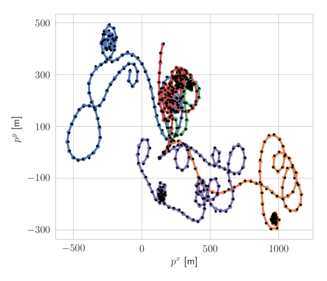
Figure 3: Five example trajectories from one noise configuration of the considered tracking problem. Each trajectory is depicted as a separate color. The black smaller dots are a specific measurement realization along each trajectory.

To evaluate the performance of each dynamically iterated filter, we calculate the average position and velocity rmse (separately) over the simulations for each of the filters and their corresponding baselines. We also compute a “relative” rmse, relative the non-iterated counterpart, i.e.,

$$V=\frac{\textsc{RMSE}_{\textrm{iter}}}{\textsc{RMSE}_{\textrm{base}}},$$ (28)

where clearly, $V\in[0,\infty]$ and lower is better. A relative score of $0.9$ thus translates to a $10\%$ lower rmse as compared to the baseline. This yields a “quick glance” picture of the expected rmse performance improvement in each particular noise configuration for each respective algorithm. For the diekf the non-iterated baseline is the ekf whereas for both the diukf and diplf the baseline is the ukf.

The results are presented as $5\times 5$ matrices where each cell corresponds to a particular noise configuration for a particular pair of algorithms, e.g., the results for the diekf and ekf are summarized in one matrix. The results can be found in Fig. 4 where the position and velocity rmses are presented in Fig. 4(a) and Fig. 4(b), respectively. The leftmost matrix in each of the figures corresponds to the diekf and ekf. The middle matrix contains the results for the diukf and ukf and the rightmost matrix for the diplf and ukf. The top number in each cell is the rmse for the dynamically iterated filter whereas the bottom number corresponds to the baseline. The color of each cell represents the rmse of the dynamically iterated filter relative its baseline, according to 28. A deeper green color thus indicates a more substantial improvement than a lighter green. Lastly, an algorithm is considered to have diverged if its position rmse is approximately larger than $\sigma$, where $\sigma$ is the measurement noise standard deviation, as a position rmse of $\sigma$ can be expected by just using the raw measurements. Divergence is illustrated by a “$-$” in the corresponding cell in the matrices.

From Fig. 4(a), it is clear that even though all of the dynamically iterated filters improve upon their baselines, the analytically linearized diekf benefits the most from the iterative procedure. Astonishingly, the ekf diverges for 22 out of 25 configurations whereas the diekf manages to lower that to 5 out of 25 and only diverges in the high noise scenario ($\sigma^{2}=${10}^{2}$$). The performance increase in position rmse is more modest for the diukf and diplf but still sees improvement, particularly for low process noise regimes. For the velocity rmse in Fig. 4(b), the improvement for all of the three dynamically iterated filters is substantial. For low process noise regimes the improvement is up to 10-fold for the diekf and 5-fold for the diukf and diplf. Even for modest noise levels, the diukf and diplf roughly manage a 2-fold performance improvement. For the high noise scenario ($\sigma^{2}=${10}^{2}$$), the diukf and diplf show a 10-fold performance improvement and bring the velocity rmse down to reasonable levels where the rmse for the ukf is very high.

((a)) Position rmse. Clearly, the analytically linearized diekf improves the most over it’s baseline the ekf which diverges in 22/25 configurations. The diukf (middle) and diplf (right) share similar performance where the diplf is slightly better for some configurations.

((b)) Velocity rmse. Clearly, all three dynamically iterated filters improve substantially over their corresponding baselines. For low noise regimes, up to 10-fold improvements are seen for the diekf whereas the diukf and diplf have approximately a 5-fold improvement. For high noise regimes the results for the diukf and diplf are even better with approximately 10-fold improvements.

Figure 4: rmse for the dynamically iterated filters as compared to their respective baselines for 25 noise configurations, where each cell corresponds to one noise configuration given by the figure axes. The top number in each cell is the rmse for the dynamically iterated filter whereas the bottom number is the rmse for the corresponding baseline. A “$-$” indicates that the positional rmse of the filter is larger than $\sigma$ and it is thus considered to have diverged, since an rmse of $\sigma$ corresponds to just using the raw measurements. The left plot in LABEL:sub@fig:positionrmse and LABEL:sub@fig:velocityrmse shows the rmse for the diekf and ekf. The middle figure shows the diukf and ukf and finally, the right most figure shows the diplf and ukf. Each cell is colored according to the rmse of the dynamically iterated filter relative to the baseline. A relative rmse of $0.9$ corresponds to a $10\%$ reduction of the rmse.

VI Conclusion

Dynamically iterated filters, a new class of iterated nonlinear filters, has been presented. The dynamically iterated filters, as opposed to previous iterated filters, are applicable to all possible combinations of (Gaussian) linear and nonlinear transition and measurement models. The filters were evaluated against their respective non-iterated baselines in a numerical example with a nonlinear transition model and a linear measurement model. Even in this “simple” case, where standard filters typically perform well, the dynamically iterated filters had improved rmse performance, especially for non-measurable states. Further, even though the ekf diverged in 22 out of 25 configurations considered, the dynamically iterated ekf was empirically shown to be stable for 20 out of 25 noise configurations, only diverging for high noise $(\sigma^{2}=${10}^{2}$)$.

Future work includes more extensive testing on other models as well as determining in what particular scenarios the statistically linearized versions perform better than the analytically and vice versa.

VII Acknowledgments

The authors would like to extend sincere gratitude to Martin Skoglund for excellent tips for the experimental evaluation.

Appendix A Loss Derivation

The kl divergence between the true joint Section IV and the approximate Section IV is given by

References

• [1] R. E. Kalman, “A New Approach to Linear Filtering and Prediction Problems,” Journal of Basic Engineering, vol. 82, no. 1, pp. 35–45, Mar. 1960.
• [2] S. Julier, J. Uhlmann, and H. Durrant-Whyte, “A New Approach for Filtering Nonlinear Systems,” in Proceedings of 1995 American Control Conference - ACC’95, vol. 3.   Seattle, WA, USA: American Autom Control Council, 1995, pp. 1628–1632.
• [3] T. Lefebvre, H. Bruyninckx, and J. De Schuller, “Comment on ”A new method for the nonlinear transformation of means and covariances in filters and estimators” [with authors’ reply],” IEEE Trans. Automat. Contr., vol. 47, no. 8, pp. 1406–1409, Aug. 2002.
• [4] A. H. Jazwinski, Stochastic Processes and Filtering Theory.   Academic Press, 1970.
• [5] M. A. Skoglund, F. Gustafsson, and G. Hendeby, “On Iterative Unscented Kalman Filter using Optimization,” in 2019 22th International Conference on Information Fusion (FUSION), Ottawa, ON, Canada, Jul. 2019, pp. 1–8.
• [6] R. Zhan and J. Wan, “Iterated Unscented Kalman Filter for Passive Target Tracking,” IEEE Trans. Aerosp. Electron. Syst., vol. 43, no. 3, pp. 1155–1163, Jul. 2007.
• [7] G. Sibley, G. Sukhatme, and L. Matthies, “The Iterated Sigma Point Kalman Filter with Applications to Long Range Stereo,” in Robotics: Science and Systems II.   Robotics: Science and Systems Foundation, Aug. 2006.
• [8] Á. F. García-Fernández, L. Svensson, M. R. Morelande, and S. Särkkä, “Posterior Linearization Filter: Principles and Implementation Using Sigma Points,” IEEE Trans. Signal Process., vol. 63, no. 20, pp. 5561–5573, Oct. 2015.
• [9] M. Raitoharju, R. Hostettler, and S. Sarkka, “Posterior Linearisation Filter for Non-linear State Transformation Noises,” in 2022 25th International Conference on Information Fusion (FUSION).   Linköping, Sweden: IEEE, Jul. 2022, pp. 1–6.
• [10] Á. F. García-Fernández, L. Svensson, and S. Särkkä, “Iterated Posterior Linearization Smoother,” IEEE Trans. Automat. Contr., vol. 62, no. 4, pp. 2056–2063, Apr. 2017.
• [11] S. Särkkä, Bayesian Filtering and Smoothing, 1st ed.   Cambridge University Press, Sep. 2013.
• [12] Á. F. García-Fernández, L. Svensson, and M. R. Morelande, “Iterated Statistical Linear Regression for Bayesian Updates,” in 17th International Conference on Information Fusion (FUSION), Salamanca, Spain, Jul. 2014, pp. 1–8.
• [13] B. M. Bell, “The Iterated Kalman Smoother as a Gauss–Newton Method,” SIAM J. Optim., vol. 4, no. 3, pp. 626–636, Aug. 1994.