Prediction-based Variable Selection for Component-wise Gradient Boosting

Abstract

Model-based component-wise gradient boosting is a popular tool for data-driven variable selection. In order to improve its prediction and selection qualities even further, several modifications of the original algorithm have been developed, that mainly focus on different stopping criteria, leaving the actual variable selection mechanism untouched. We investigate different prediction-based mechanisms for the variable selection step in model-based component-wise gradient boosting. These approaches include Akaikes Information Criterion (AIC) as well as a selection rule relying on the component-wise test error computed via cross-validation. We implemented the AIC and cross-validation routines for Generalized Linear Models and evaluated them regarding their variable selection properties and predictive performance. An extensive simulation study revealed improved selection properties whereas the prediction error could be lowered in a real world application with age-standardized COVID-19 incidence rates.

Keywords gradient boosting, variable selection, prediction analysis, high-dimensional data, sparse models

1 Introduction

In regression settings with a large number of possible covariates, tools for proper variable selection are useful. One popular tool for data-driven variable selection are model-based component-wise gradient boosting algorithms [1], which emerged in the statistical learning community within the last two decades.

The main idea of the first boosting algorithm AdaBoost [2] was to fit several simple classifiers and combine these “weak learners" to a single strong learner with a very good predictive performance. Boosting is therefore also referred to as an ensemble learning technique. Based on the observation that AdaBoost minimizes some loss function [3], it has been shown that boosting can be represented in the statistical framework of Generalized Additive Models (GAMs) [4]. This allows for more flexibility in terms of loss functions and weak learners such as ordinary-least squares (OLS) fits or splines. Combining boosting with gradient descent techniques to iteratively minimize loss functions made the boosting approaches even more powerful [5]. Despite its implicit variable selection, model-based component-wise gradient boosting algorithm as proposed by Bühlmann and Hothorn [1], results in a good predictive performance. It combines further advantages like fast computation, coefficient shrinkage and model choice as well as the applicability in high-dimensional settings, where the number of covariates exceeds the number of observations and offers a flexible framework, that can be used for various applications. Since we apply model-based component-wise gradient boosting we refer to it as boosting from now on.

Boosting is a statistical learning mechanism, that iteratively estimates the coefficient vector of a given regression model. To do so, it refits simpler estimation procedures on the (pseudo-)residuals of the previous iteration, which can be seen as the gradient of a differentiable loss function. In the case of Generalized Linear Models (GLMs), this loss is usually chosen as the negative of the corresponding log-likelihood. For each iteration, the model fit is updated in a component-wise fashion, i.e. every single covariate is fitted separately and the algorithm identifies and updates the covariate whose update reduces the loss function the most.

The boosting procedure is run for a rather large pre-specified number of iterations. Following, for every iteration-specific coefficient vector, prediction criteria can be calculated. This allows to select the best performing coefficient vector in the aftermath. If some covariates did not enter the model up to the selected iteration, they are excluded from the final model. Furthermore, selecting the best iteration controls the bias-variance trade-off and thus enables coefficient shrinkage.

There exist several modifications of the original boosting algorithm, that aim to optimize its performance even further, e.g. to lower the false positive rate (FPR) such that only true influential variables enter the final model: The AIC-subsampling approach [6] as well as the probing method [7] focus on a fully data-driven iteration selection.

Stability selection [8, 9], deselection [10] and Twin-boost [11] concentrate on filtering the main influential covariates by enlarging the number of boosting rounds. Other approaches [12] allow for multivariate updates and use a double-checking mechanism to decrease the FPR.

The majority of approaches mainly focuses on different stopping criteria, leaving the actual variable selection mechanism untouched. Since boosting is a greedy algorithm this variable selection step is of major importance. Thus, in this paper we investigate the variable selection step in order to increase the sparsity of boosted GLMs without sacrificing the good predictive performance.

Only few other papers deal with modifications of the variable selection step. One approach modified the variable selection criterion from the traditional loss function to the generalized minimum description-length (gMDL) concept to generate sparser models [13]. When compared to conventional squared-error loss boosting, Sparse$L_{2}$Boosting with a gMDL variable selection produces sparser models with equivalent predictive performance, and is especially effective in high-dimensional settings. In the framework of unbiased model selection in boosting with different kinds of covariates, it has been proposed to select the base learner using the AIC [14]. However, this does not result in an unbiased model selection in the case of base learners with very different degrees of freedom (e.g. categorical variable with ten categories vs. one metric variable with the same kind of base learner). The AIC-based variable selection for likelihood-based boosting has been implemented by Tutz and Groll in the special case of Generalized Linear Mixed Models [15] and there may be differences in behaviour on GLMs owing to the error variance decomposition in mixed models.

There is, however, a lack of a systematic investigation of the modification of the variable selection step in gradient boosted GLMs which this paper will address. Therefore, two different prediction-based variable selection mechanisms are presented and evaluated in the following in order to examine their impact on sparsity of gradient boosted GLMs. Instead of minimizing a loss function, our approach focuses on minimizing various prediction criteria directly.

The rest of the paper is structured as follows: in the second section, model-based component-wise gradient boosting for GLMs is described in more detail and our extension of the concept is explained. In section three a simulation study is conducted to evaluate the new procedures and the results are presented. Section four deals with modelling a real world data set on COVID-19 incidence rates. In section five the results of this paper are summarized and an outlook on possible extensions is given.

2 Prediction-based variable selection

Investigating the variable selection step of boosting is motivated by its direct impact on the variable selection process compared to a more downstream impact of the boosting iteration selection. The selection of the variable to be updated in boosting algorithms usually employs the loss function. Based on the promising findings using the gMDL-criterion [13], this paper investigates two different variable selection criteria for boosting of GLMs.

Pulling the former iteration-selection criteria into the variable selection loop of the algorithm may prevent the inclusion of false positives (FPs) already during the fitting process. Since boosting is a greedy algorithm, i.e. once a variable enters the model, it will be included in every following iteration, it is even more important to take a closer look at the variable selection step. In this section we will explain our modification of this selection step by lining out the changes in the algorithm.

Based on the given data $\mathcal{D}:=\{(\boldsymbol{x}_{1},y_{1}),(\boldsymbol{x}_{2},y_{2}),\ldots,(\boldsymbol{x}_{N},y_{N})\}$ an iterative algorithm is run. The data can be rewritten as a design matrix $\boldsymbol{X}\in\mathbb{R}^{N\times(k+1)}$ summarizing all observations $\boldsymbol{x}_{i}=(x_{i0},x_{i1},x_{i2},\ldots,x_{ik})^{\prime}$ with $x_{i0}=1$, $i=1,\dots,N$, $j=1,\dots,k$ and an outcome vector $\boldsymbol{y}\in\mathbb{R}^{N}$, with $k\in\mathbb{N}$ being the number of covariates and $N\in\mathbb{N}$ the number of observations.

The algorithm is run for $T$ iterations where each iteration-specific argument is marked by $(\cdot)^{(t)}$ with $t\in\{0,1,\ldots,T\}$. It is assumed that the regression problem can be written as a GLM, where the negative Log-likelihood serves as a loss function for the boosting algorithm in order to estimate the vector of the true coefficients $\boldsymbol{\beta}\in\mathbb{R}^{k+1}$.

Both upcoming prediction-based variable selection mechanisms possess the advantage, that they do not need further time-consuming computations to determine the final stopping iteration. Since they incorporate a prediction-based measure, which is evaluated for each covariate in every iteration, the global minimum of the $k\times T$ candidates can be used to define the stopping iteration

$$t^{*}=\underset{c~{}\in\{1,\ldots,k\times T\}}{\operatorname{argmin}}\text{crit}_{c}.$$ (1)

The selection is done, after the $T$ iterations were run. However, in order to favor sparser models, a minimum improvement threshold of $10^{-8}$ is specified. If the change in the prediction criterion or the $\boldsymbol{\hat{\beta}}$ vector between two iterations $t$ and $t+1$ is smaller than the threshold, iteration $t$ is selected even though $t+1$ yields the analytical minimum. The value of the threshold is chosen rather arbitrarily to stop fitting if changes become too small.

2.1 Cross-validation (CV)

The first option makes use of an ($F$-fold) CV procedure. The algorithm is essentially identical to boosting, except the variable selection part displayed in Algorithm 1. It allows for a stable prediction-based evaluation of the best fitting covariate. Once the optimal covariate-index $j^{*}\in\{1,\dots,k\}$ is identified, $\boldsymbol{\hat{\beta}}^{(t)}$ is updated based on the corresponding base learner using all data again.

for j in $1:k$ do

     for f in $1:F$ do

         calculate $j$-th base learner on all but fold $f$ base learner: ${\hat{\beta}_{j,-f}^{(t)}}=\left(\left(\boldsymbol{x}_{(j),-f}\right)^{\prime}\boldsymbol{x}_{(j),-f}\right)^{-1}\left(\boldsymbol{x}_{(j),-f}\right)^{\prime}\boldsymbol{u}^{(t)}_{-f}$

         update $j$-th entry of ${\boldsymbol{\hat{\beta}}^{(t-1)}}$ by the base learner using step length parameter $\nu$ resulting in ${\boldsymbol{\tilde{\beta}}_{j,-f}^{(t)}}$

         evaluate loss function with ${\boldsymbol{\tilde{\beta}}_{j,-f}^{(t)}}$ and data from fold $f$ $l_{j_{f}}=L\left(\boldsymbol{y}_{{f}},\boldsymbol{X}_{{f}}{\boldsymbol{\tilde{\beta}}_{j,-f}^{(t)}}\right)$

     end for

     get mean loss over the folds $\displaystyle{\bar{l_{j}}=\frac{1}{F}\sum_{f=1}^{F}l_{j_{f}}}$

end for

choose $\displaystyle{j^{*}=\underset{j~{}\in\{1,\ldots,k\}}{\operatorname{argmin}}~{}\bar{l_{j}}}$

Algorithm 1 Cross-validation Variable Selection in Component-wise Gradient Boosting

2.2 Akaike Information Criterion (AIC)

As a second option the AIC can be used in the variable selection step. This approach has been successfully integrated in likelihood-based boosting for Generalized Linear Mixed Models [15]. In order to include the AIC into the boosting procedure, a definition of the degrees of freedom (df) is needed. In a usual multivariate GLM the df correspond to the number of included parameters $k+1$ which equals the rank of the design matrix $\boldsymbol{X}$. The common way to derive the df of a GLM is to compute the trace of the hat matrix. Thus, a specification of the hat matrix for the boosting algorithm is needed which has been derived by Bühlmann and Hothorn [1] and is displayed in Equation (2). We restrict the explanation to the df for OLS base learners, since other base learners are not applied throughout the paper.

$$\boldsymbol{B}^{(t)} = \boldsymbol{B}^{(t-1)}+\nu\cdot\boldsymbol{H}_{j^{*}_{t}}\left(\boldsymbol{I}-\boldsymbol{B}^{(t-1)}\right)$$ (2)

$$= \boldsymbol{I}-\left(\boldsymbol{I}-\nu\boldsymbol{H}_{j^{*}_{t}}\right)\cdot\left(\boldsymbol{I}-\nu\boldsymbol{H}_{j^{*}_{t-1}}\right)\cdots\Big{(}\boldsymbol{I}-\nu\boldsymbol{H}_{j^{*}_{1}}\Big{)},$$

with $j^{*}_{t}\in\{1,\ldots,k\}$ representing the selected covariate in iteration $t$. Similarly, $\boldsymbol{H}_{j^{*}_{t}}$ corresponds to the hat matrix of the covariate $j^{*}_{t}$ together with an intercept. To account for the response function $h(\boldsymbol{\eta}_{i})$ used in GLMs, a weighting matrix $\boldsymbol{W}=\text{diag}(w_{1},\ldots,w_{N})$ with $w_{i}=(\partial h(\eta_{i}))^{2}/\text{var}(y_{i})$ has to be included in Equation (2) resulting in

$$\boldsymbol{B}^{(t)} = \boldsymbol{B}^{(t-1)}+\nu\cdot\boldsymbol{W}\boldsymbol{H}_{j^{*}_{t}}\left(\boldsymbol{I}-\boldsymbol{B}^{(t-1)}\right)$$

$$\text{df}^{(t)} \approx \text{tr}(\boldsymbol{B}^{(t)}).$$ (3)

The derivation of $\boldsymbol{W}$ follows from the Maximum-Likelihood estimation of a GLM [16]. Bühlmann and Hothorn emphasized that $\boldsymbol{B}^{(t)}$ can only be seen as an approximation of the hat matrix, since it depends on $\boldsymbol{y}$ due to the iterative selection of $j^{*}$ [1]. A comment of Hastie [17] points out, that this procedure underestimates the true degrees of freedom still leading to a tendency of AIC stopping criteria to overfit the training data.

for j in $1:k$ do

     update $j$-th entry of ${\boldsymbol{\hat{\beta}}^{(t-1)}}$ by the base learner of the $j$-th variable using step length parameter $\nu$ resulting in ${\boldsymbol{\tilde{\beta}}^{(t)}_{j}}$ base learner: ${\hat{\beta}_{j}^{(t)}}=\left(\left(\boldsymbol{x}_{(j)}\right)^{\prime}\boldsymbol{x}_{(j)}\right)^{-1}\left(\boldsymbol{x}_{(j)}\right)^{\prime}\boldsymbol{u}^{(t)}$

     evaluate $\text{AIC}_{j}=-2\times\text{log}\ \mathcal{L}\left({\boldsymbol{\tilde{\beta}}^{(t)}_{j}}\right)+2\times\text{df}^{(t)}_{j}$

end for

choose $\displaystyle{j^{*}=\underset{j~{}\in\{1,\ldots,k\}}{\operatorname{argmin}}~{}\text{AIC}_{j}}$ and calculate $\boldsymbol{B}^{(t)}$ from Eq. (2.2)

Algorithm 2 AIC Variable Selection in Component-wise Gradient Boosting

Despite its imprecise measure of the df, the AIC still penalizes more complex models stronger and is hence used as an extension of approaches solely based on the loss function. Therefore, the AIC is taken as a second option of the variable selection criterion and can be implemented as seen in Algorithm 2. The degrees of freedom $\text{df}^{(t)}_{j}$ can be calculated as shown in Equation (2.2).

$$\boldsymbol{B}^{(t)}_{j} = \boldsymbol{B}^{(t-1)}+\nu\cdot\boldsymbol{W}\boldsymbol{H}_{j}\left(\boldsymbol{I}-\boldsymbol{B}^{(t-1)}\right)$$

$$\text{df}^{(t)}_{j} \approx \text{tr}\left(\boldsymbol{B}^{(t)}_{j}\right).$$ (4)

For the purpose of shorter computation time, we may apply $\text{tr}(\boldsymbol{A}\boldsymbol{B})=\text{sum}(\boldsymbol{A}\cdot\boldsymbol{B})$ in the inner $j$-loop with $(\cdot)$ referring to element-wise multiplication because these calculations only require the trace of $\left(\boldsymbol{H}_{j}\left(\boldsymbol{I}-\boldsymbol{B}^{(t-1)}\right)\right)$. Nevertheless, as $\boldsymbol{B}^{(t-1)}$ is needed for calculations in $t$ (and not only its trace), one matrix multiplication of the $N\times N$ matrices shown in Equation (2.2) has to be performed in each iteration $t$.

Replacing the AIC in Algorithm 2 with the loss function would yield the classical model-based component-wise gradient boosting algorithm.

3 Simulations

3.1 Setup

The performance of the two new prediction-based variable selection mechanisms is examined in a simulation study. The benchmark model is generated via mboost [18] using the glmboost command with 10-fold CV. The study investigates various scenarios with fixed number of observations $N=250$, where the values of the design matrix are drawn from a multivariate normal distribution with different settings, i.e.

$$\boldsymbol{X}\sim\text{MVN}(\boldsymbol{0},\boldsymbol{\Sigma}),\text{ where }\boldsymbol{\Sigma}\in\left\{\boldsymbol{I}_{k},\boldsymbol{\Sigma}_{k}^{\text{Toep}}\right\}\text{ and }k\in\{100,500\}.$$

$\boldsymbol{I}_{k}$ represents the identity matrix and $\boldsymbol{\Sigma}_{k}^{\text{Toep}}$ holds the elements $\text{Cov}\left(\boldsymbol{x}_{(p)},\boldsymbol{x}_{(q)}\right)=0.9^{|p-q|},\forall~{}p\in\{1,\ldots,k\}$ and $q\in\{1,\ldots,k\}$. An intercept column is added to $\boldsymbol{X}$. Further, the outcome variable is set to be normally distributed

$$y_{i}=\beta_{0}x_{i0}+\sum_{r=1}^{\text{INF}}x_{ir}\beta_{r}+\varepsilon_{i}\text{ with }\varepsilon_{i}\overset{\text{iid}}{\sim}\mathcal{N}(0,1)\text{ and }\beta_{0}=1$$

and $\text{INF}\in\{5,20\}$. The true coefficients are scaled, in order to achieve pre-defined levels of the noise-to-signal ratio (NSR) [19]. The scaling works as follows

$$\beta_{r}=\kappa\tilde{\beta}_{r},\text{ where }\tilde{\beta}_{r}\sim\mathcal{U}(\{-3,-2,-1,1,2,3\})$$

with the scaling factor $\kappa$, which is defined as

$$\kappa=\sqrt{\frac{1}{\text{NSR}\boldsymbol{\tilde{\beta}}\boldsymbol{\Sigma}\boldsymbol{\tilde{\beta}}}}\text{, where }\boldsymbol{\tilde{\beta}}=\big{(}\tilde{\beta}_{r}\big{)}_{1\leq r\leq\text{INF}}\text{ and }\text{NSR}=\frac{\mathrm{Var}(\boldsymbol{\varepsilon})}{\mathrm{Var}(\boldsymbol{X\beta})}\in\{0.2,0.5,1\}.$$

Thus, the simulation study uses a varying number of covariates $k\in\{100,500\}$, varying NSRs $\text{NSR}\in\{0.2,0.5,1\}$, different amounts of true positive covariates ${\text{INF}}\in\{5,20\}$ and two correlation structures of the covariates $\boldsymbol{\Sigma}\in\left\{\boldsymbol{I}_{k},\boldsymbol{\Sigma}_{k}^{\text{Toep}}\right\}$. The configurations result in 12 low-dimensional ($k<N$) and 12 high-dimensional ($k>N$) settings, as seen in Table 2.

The number of true positives (TPs) covariates INF is chosen to vary, in order to provide different levels of true sparsity. To simulate settings in which the true influential covariates vary in difficulty of identification, the NSR is selected to vary from low (easier detection) to high (harder detection). Further, two types of correlation structure are examined to uncover possible different behaviours of the algorithms. For every setting 100 simulation runs are executed. To evaluate the out-of-sample predictive performance the models are tested on 100 additional data points evolving the same data generating process. The chosen evaluation criteria regarding variable selection properties and quality of prediction are the FPR and the mean squared prediction error (MSPE), respectively. Further the true positive rate (TPR), the number of iterations and the ratios of the average computation time are evaluated.

All algorithms are trained for $T=3000$ boosting iterations with a step-length parameter $\nu=0.1$. The baseline model and the newly proposed CV variable selection method use ten folds. All models start with an offset of $\bar{y}$, i.e. an intercept-only model.

The following section evaluates the performance of the two modifications in the simulation study and compares them to the benchmark. To emphasize that mboost employs the prediction criteria after fitting the model, whereas the modifications directly include their calculation during the fitting process, the criteria are added at the end ($\text{mboost}_{\text{CV}}$) or at the beginning (AIC-boost, CV-boost) of their names, respectively.

3.2 Results

The results of the simulations are split up into the examined indicators and are displayed and described in the following. The included figures show results for the uncorrelated cases and plots covering both correlation structures can be found in the Appendix A.1.

False positive rate

Regarding the FPR, we observe the following trend visualized in Figure 1: The AIC-variable selection (AIC-boost) outperforms both, mboost with 10-fold CV ($\text{mboost}_{\text{CV}}$) and CV-boost in most of the tested scenarios, e.g. in case of uncorrelated covariates with $k=500$, ${\text{INF}}=5$ and $\text{NSR}=0.2$ (bottom left, first x-axis entry). In this setting, CV-boost results in a median FPR of around 0.43, while $\text{mboost}_{\text{CV}}$ yields an FPR of 0.04. The median FPR of the AIC-method is 0.01 in the described setting, which is the lowest of the three algorithms.

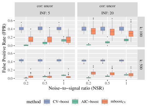
Figure 1: False Positive Rate for new variable selection strategies by simulation setting.

This pattern can be found in nearly all tested settings of the simulation study, however little differences are worth to highlight: the variability of the FPR of the two new algorithms is substantially lower than $\text{mboost}_{\text{CV}}$ in every setting. Due to the relative nature of the FPR, one has to be cautious with comparisons between the low-dimensional and the high-dimensional setting. The variability of the FPR in the high-dimensional setting appears smaller, but equal measures of location and scale of the FPR would yield different absolute values (i.e. FPs) depending on the dimensionality.

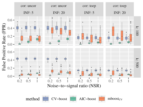
Figure 5: False Positive Rate for new variable selection strategies by simulation setting.

Another observation concerns the true sparsity of the models, which is varied by INF. It appears, that the performance of $\text{mboost}_{\text{CV}}$ depends on the true sparsity. Enlarging the number of true informative covariates and keeping the other parameters constant results in a higher FPR of $\text{mboost}_{\text{CV}}$, whereas the two modifications perform more robust and reveal very similar FPR across the differing numbers of informative covariates. This pattern is more pronounced in the uncorrelated settings (see column 1 and 2 in Figure 5).

Table 1: Comparison of False Positive Rates of AIC-boost and $\text{mboost}_{\text{CV}}$ by noise-to-signal ratio.

	settings with superior performance∗ of AIC-boost compared to $\text{mboost}_{\text{CV}}$
	Number	Percentage
NSR = 0.2	8/8	100%
NSR = 0.5	7/8	88%
NSR = 1	4/8	50%

Superior performance is measured by means of the median FPR.

The performance of the AIC-method looks promising, since it outperforms $\text{mboost}_{\text{CV}}$ in 19/24 ($79\%$) settings in terms of the median FPR. A detailed listing can be found in Table 5. It summarizes the number of settings by parameter in which AIC-boost has a lower median FPR than the benchmark $\text{mboost}_{\text{CV}}$. The most influential parameter appears to be the NSR (see Table 1 and Table 5). AIC-boost always results in sparser models when $\text{NSR}=0.2$ is used, regardless of high or low dimension and the amount of informative covariates. Contrary, simulation settings with $\text{NSR}=1$ result in a share of only 4/8 ($50\%$) settings, where AIC-boost outperforms the benchmark model. Thus, in situation with strong signal, AIC-boost is more likely to outperform $\text{mboost}_{\text{CV}}$ than in weak signal situations. Generally, AIC-boost performs better in settings with a high signal compared to weak signal settings. A reason for this may be the difference between the contributions of TPs and FPs: In strong signal situations, the contribution of the true positives to minimize the loss function exceeds the smaller contributions of FP to a large extend. The penalty term of the AIC ensures, that the model refrains from including them, until the contribution of the TP becomes small enough. In weak signal situations the contributions of TPs and FPs do not differ so much and thus, the algorithm includes more FPs.

In terms of the FPR, the simulation study clearly recommends using the newly tested AIC-boost in low-dimensional settings for both correlation structures. In high-dimensional data settings, the performance is determined by the NSR. However, in 8/12 high-dimensional settings AIC-boost outperforms $\text{mboost}_{\text{CV}}$. The variability of the FPR is drastically reduced in every tested simulation set-up (see Figure 1 and Table 2), which suggests that AIC-boost is a more robust estimation procedure in terms of the FPR.

Table 2: Median (variance $\times$ 100) FPR and TPR for AIC-boost and $\text{mboost}_{\text{CV}}$ by simulation setting.

				FPR		TPR
correlation	k	INF	NSR	AIC-boost	$\text{mboost}_{\text{CV}}$	AIC-boost	$\text{mboost}_{\text{CV}}$
uncorrelated	100	5	0.2	0.011 (0.014)	0.126 (0.739)	1.000 (0.000)	1.000 (0.000)
			0.5	0.074 (0.085)	0.126 (0.737)	1.000 (0.000)	1.000 (0.000)
			1	0.137 (0.114)	0.126 (0.789)	1.000 (0.055)	1.000 (0.133)
		20	0.2	0.025 (0.022)	0.356 (1.215)	0.952 (0.272)	1.000 (0.013)
			0.5	0.075 (0.094)	0.331 (1.263)	0.905 (0.415)	0.952 (0.182)
			1	0.138 (0.162)	0.288 (1.234)	0.810 (0.420)	0.905 (0.483)
	500	5	0.2	0.010 (0.003)	0.037 (0.120)	1.000 (0.000)	1.000 (0.000)
			0.5	0.041 (0.010)	0.037 (0.124)	1.000 (0.028)	1.000 (0.082)
			1	0.075 (0.015)	0.032 (0.106)	1.000 (0.296)	1.000 (0.609)
		20	0.2	0.015 (0.004)	0.131 (0.210)	0.952 (0.236)	1.000 (0.116)
			0.5	0.052 (0.011)	0.115 (0.207)	0.857 (0.424)	0.905 (0.529)
			1	0.085 (0.016)	0.088 (0.202)	0.762 (0.550)	0.762 (1.077)
Toeplitz correlation	100	5	0.2	0.011 (0.011)	0.200 (1.418)	1.000 (1.485)	1.000 (1.015)
			0.5	0.032 (0.039)	0.158 (1.549)	0.833 (1.588)	0.833 (1.958)
			1	0.053 (0.063)	0.100 (1.288)	0.833 (2.153)	0.833 (2.706)
		20	0.2	0.013 (0.019)	0.350 (2.203)	0.571 (1.594)	0.833 (2.109)
			0.5	0.038 (0.059)	0.200 (2.178)	0.571 (1.823)	0.667 (2.579)
			1	0.050 (0.090)	0.125 (1.842)	0.524 (1.420)	0.524 (2.394)
	500	5	0.2	0.007 (0.002)	0.069 (0.368)	1.000 (1.031)	0.833 (1.915)
			0.5	0.024 (0.007)	0.043 (0.230)	1.000 (1.459)	0.833 (2.666)
			1	0.042 (0.009)	0.020 (0.174)	0.833 (1.948)	0.667 (2.547)
		20	0.2	0.008 (0.005)	0.073 (0.476)	0.571 (1.814)	0.571 (1.630)
			0.5	0.025 (0.009)	0.035 (0.185)	0.524 (1.452)	0.429 (1.238)
			1	0.044 (0.016)	0.020 (0.131)	0.476 (1.197)	0.381 (1.290)

True positive rate

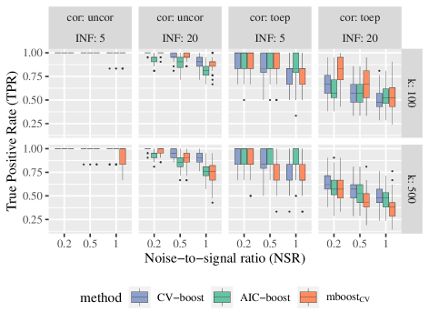
Figure 7: True Positive Rate for new variable selection strategies by simulation setting.

Another trend can be observed when looking at the TPR in Table 2 and Figure 7: In settings with just ${\text{INF}}=5$ informative covariates, the AIC-boost yields very good (median) TPR, which are always better or equal compared to $\text{mboost}_{\text{CV}}$. In settings with ${\text{INF}}=20$ informative covariates AIC-boost reveals the tendency to have a lower median TPR than the baseline method (7/12 scenarios). Differences are less pronounced in the uncorrelated settings ($\approx$ five percentage points worse). Note, the TPR can be compared between low- and high-dimensional settings, as it only depends on INF and not on $k$. Using 20 informative Toeplitz-correlated covariates, AIC-boost outperforms $\text{mboost}_{\text{CV}}$ in the high-dimensional setting, whereas this relationship is reversed in the low-dimensional cases.

CV-boost does not show a clear trend in terms of TPR. It eventually outperforms AIC-boost and the benchmark model, e.g. Toeplitz correlated case with $k=500,\text{NSR}=0.2,{\text{INF}}=20$ and sometimes reveals a TPR similar to AIC-boost. While the FPR is clearly reduced by AIC-boost, this is not recognizable with the same degree of certainty for the TPR.

In summary, the much lower FPR for AIC-boost is accompanied by a slightly lower TPR in some setups.

Mean squared prediction error

Since prediction and sparsity were seen as two opposing aims in model selection processes, the next indicator to analyze is the MSPE. Despite the fact that AIC-boost often results in sparser models, which increases the interpretability, it still keeps up with the benchmark model in terms of prediction accuracy (see Figure 2). CV-boost produces slightly (considerably) higher median MSPE in low-dimensional (high-dimensional) settings with uncorrelated covariates. Using the Toeplitz covariance structure, differences between the three methods are less pronounced. Thus, applying the AIC-boost approach results in sparser models without sacrificing the predictive performance of the model in the vast majority of scenarios.

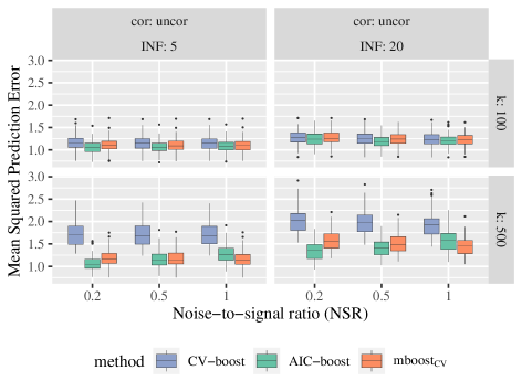
Figure 2: Mean Squared Prediction Error for new variable selection strategies by simulation setting.

Number of iterations and computation time

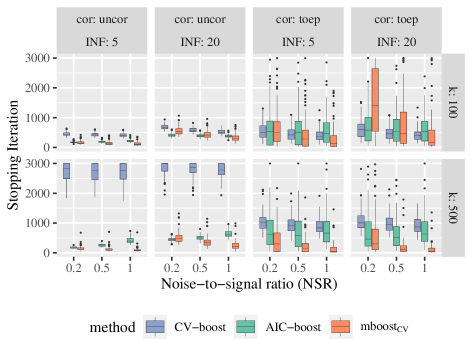
Figure 8: Stopping iteration $t^{*}$ for new variable selection strategies by simulation setting.

Looking at the selected stopping iteration (Figure 8), $\text{mboost}_{\text{CV}}$ always exhibits the lowest median in terms of stopping iteration. After looking at the higher FPR of $\text{mboost}_{\text{CV}}$ one would probably expect the contrary – a later stopping iteration, meaning more possibilities to include FPs. But since the modification of the variable selection step changes the pattern in the coefficient paths (see Figure 3), earlier stopping iterations of $\text{mboost}_{\text{CV}}$ can yield more included covariates when compared to AIC-boost at the same iteration. Figure 3 illustrates coefficient paths of the two modifications and the baseline model exemplarily. The figure results from one simulation run with Toeplitz correlated covariates in a Gaussian setting using $k=100$, $\text{INF}=5$ and $\text{NSR}=0.2$. It can be seen, that changing the variable selection step influences how many covariates enter the final model. Further, the size of the coefficients and the order of inclusion may be affected. The coefficient paths of AIC-boost (Figure 3 middle) are the steepest and its resulting final model includes the least FPs.

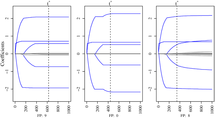
Figure 3: Coefficient paths of CV-boost (left), AIC-boost (middle) and $\text{mboost}_{\text{CV}}$ (right). Blue paths correspond to true influential covariates, grey represents false positives.

The most influential parameter of the simulation governing the computation time of the algorithms (beside the number of observations which is held constant) is the number of possible covariates $k$. Table 3 displays the ratio of the average computation time for the two new algorithms compared to $\text{mboost}_{\text{CV}}$ in low and high-dimensional settings. The algorithms were run on an AMD EPYC 7742 Processor with two sockets. Each socket includes 64 cores with two threads per core and overall 512 GB RAM.

Table 3: Ratio of average computation time of one simulation run by number of covariates (algorithm/$\text{mboost}_{\text{CV}}$).

	CV-boost	AIC-boost
k=100	1151	142
k=500	9261	310

Clearly, both new algorithms take longer than the benchmark method. As expected CV-boost takes the longest. Note, that besides the calculation rules for AIC-boost mentioned above, no attempts were made to make the algorithms more efficient. Contrary, mboost is an optimized package.

4 Data

4.1 Data Explanation

To evaluate the two modified algorithms in a more realistic setting, they were applied to a real world data set. Therefore, a subset of a COVID-19 data base from Doblhammer et al. is used [20]. The authors investigated the relationship of county-scale variables on the county-specific age-standardized COVID-19 incidence rates in Germany in order to uncover possible social disparities. In this framework, they focussed on different periods of the pandemic in Germany and identified the ten most important county-scale covariates for each of the five periods of the pandemic in Germany by means of SHAP values. The used subset of their data contains 163 variables measured on 401 counties in Germany. The variables cover different socioeconomic characteristics, like demography, social economic and settlement structure, health care, poverty, unemployment, politics and education, interrelationship with other regions, e.g. percentage change of persons from 2012 to 2017, old-age (65+) dependency ratio (2017), total fertility rate (2017), unemployment rate (2017), persons per square kilometer (2017) or share of area in natural state (2017). By looking at the correlation structure of the possible covariates in Figure 4 (left), one can observe highly (positive and negative) correlated blocks of variables (e.g. “share of employed persons in tertiary sector in all dependently employed persons" has a Pearson correlation coefficient of $\approx-0.93$ with “share of employed persons in secondary sector in all dependently employed persons" and “unemployment rate" correlates by $\approx 0.94$ with “share of persons with basic social security benefits per 1,000 persons") corresponding to thematically-related covariates. All variables are either metric or dummy-coded. Metric covariates are standardized. The outcome of interest is the age-standardized incidence rate on the county-level for the first lockdown period (March 16,2020 - March 31,2020) as defined by Doblhammer et al. [20]. It follows a log-normal distribution (Figure 4 right).

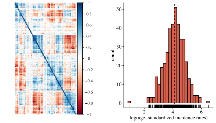
Figure 4: COVID-19 data set descriptives: correlation matrix of COVID-19 data set (left), empirical distribution of log(age-standardized incidence rates) (right).

4.2 The Model

In order to extract the most influential macro-variables associated with the log-transformed age-standardized COVID-19 incidence rates out of the pool of 163 covariates, we apply the two modified algorithms and compare their performance to mboost with 10-fold CV ($\text{mboost}_{\text{CV}}$). For reasons of comparability, $\text{mboost}_{\text{CV}}$ and CV-boost are trained using the same folds. Since these two algorithms were highly dependent on the data split, they are run five times with different data splits and median values are reported. The calculation of the MSPE is based on 100 randomly chosen data points, such that the models are trained with 301 observations. Note, that the chosen covariates may differ from the ones identified by the original article [20], since they used gradient boosting for prediction with tree-based weak learners, whereas this paper applies model-based component-wise gradient boosting with OLS base learners. The latter mentioned implies the assumption of a true linear relationship between the covariates and the log-transformed age-standardized incidence rate.

The results contradict the main message of the simulation study in terms of sparsity, as one would expect $\text{mboost}_{\text{CV}}$ to include more variables than AIC-boost.

Table 4: Performance of algorithms on COVID-19 data set.

method	stopping iteration	no. of covariates	MSE	MSPE
$\text{mboost}_{\text{CV}}$ $\dagger$	20	8	0.232	0.365
$\text{mboost}_{\text{AIC}}$	2039	85	2.553	2.801
LASSO-AIC	/	10	0.211	0.342
AIC-boost	164	21	0.154	0.296
CV-boost $\dagger$	447	53	0.140	0.281

model averaging performed, median values are reported.

However, $\text{mboost}_{\text{CV}}$ includes only nine covariates while the model using AIC-boost contains 21 covariates. This high sparsity of $\text{mboost}_{\text{CV}}$ comes along with a poorer predictive performance regarding the MSE and MSPE. Both tested algorithms outperform $\text{mboost}_{\text{CV}}$ regarding the predictive performance but include (many) more variables than the baseline model. They also outperform LASSO with an AIC stopping criterion in terms of prediction accuracy. Comparing only the two newly tested algorithms, the predictive performance is very similar by differing numbers of included covariates. Applying Occam’s razor, AIC-boost combines the sparsest model with a comparable prediction accuracy and thus would be the preferred model in this application.

4.3 Interpretation of Coefficients

During the first COVID-19 wave, there was a change in the association of socioeconomic status (SES) and incidence rates. A positive correlation could be shown between SES and high incidence rates in the early phase, whereas higher incidence rates were associated with low SES in the later phase [21, 22]. Reasons for this included higher mobility (e.g. skiing vacations) in the higher SES groups in the early periods before the introduction of government mitigation measures and less flexible working conditions in the lower SES groups later in the first wave [23]. The period from March 16 to March 31 was marked by strict lockdown measures to avoid personal contact. Table 6 displays the covariates and their coefficients for the three sparsest models. For $\text{mboost}_{\text{CV}}$ five of the 8 selected variables are consistent with the ten most important variables identified in the original article [20] and share the same direction of influence (positive/negative) on the outcome variable with the SHAP value-based approach. Two further selected variables (“Persons in long-term care per 10.000 persons in 2017” and “%Households with low income (1,500€ per month) in all households in 2016”) are equivalent indicators (Care_allowance_receivers and Social_security_benefits) covering same dimensions (poor health and households with low income). Only the variable “Premature mortality” is not covered by Doblhammer et al. [20], whereby premature mortality is higher in socioeconomically weaker areas [24] and is thus consistent with the background of a positive social gradient. The ranking of covariates in terms of the absolute value of the coefficients is very similar between LASSO and $\text{mboost}_{\text{CV}}$. However, the LASSO selection contains two more variables. The variable “Ever 100+ inbound commuters from Tirschenreuth” represents the connection/mobility to county of Tirschenreuth, which was a hotspot area with the highest incidences at this period, and increased even further since the start of March [25]. The variable “%Older employed persons (55 years+) in all employed persons” represents aging differences between the counties which is accompanied by structural weakness. This may indicate a positive social gradient as well as a geographical aspect. In recent years, aging and population shrinking in the rural eastern regions has been faster than in other rural areas [26]; whereas, incidences were lower there than in other regions during the observation period. AIC-boost incorporates several coefficients with a rather large absolute value, that are not even included in the other model. Three of these variables regard outbound commuters to hotspot areas during this period (“Ever 100+ inbound commuters…"). The variables concerning the number/share of employed persons in the younger/older/general population (“%Young employed persons in all young persons (under 26 years) in 2017”, “%Older employed persons in all older persons (55 years+) in 2011-2017”, and “%Change of number of employed persons in 2012-2016”) indicate the level of employment and are consistent with a positive social gradient, indicated by the positive sign. While there tended to be no differences in incidence between the sexes during the course of the pandemic [27], differences in infection rates between men and women appeared in the early phase of the pandemic [28]. Younger women had higher infection rates during this phase [29, 30]. The variable “%Change of number of persons at age 50-65 in 2012-2017” indicates population growth which is stronger in the south respectively partly negative in rural areas in eastern Germany where structural and economic indicators are low [31, 32]. The variables “Average travel time to the next large-sized regional center (Oberzentrum)” and “%Outbound commuters…” represent the rurality of counties. In contrast to the orginal article [20], indicators for rurality are correlated with lower incidence rates here.

Note, that no causal relationships on a sociological micro-level can be extracted here, since both, the outcome variable and the covariates are macro-indicators. Ignoring this, would lead to the ecological fallacy [33].

5 Conclusion

Based on promising findings [15, 13] and due to the lack of a systematic investigation on different variable selection mechanisms in gradient boosted GLMs, this paper evaluated two modifications of component-wise gradient boosting. Instead of minimizing the loss function in model-based boosting, two prediction-based criteria were used instead, namely: cross-validation (CV-boost) and Akaikes Information Criterion (AIC-boost). The new modifications directly minimize these criteria and were expected to reduce the false positive rate (FPR).

The simulation study with a normally distributed outcome revealed that CV-boost does not outperform the benchmark model $\text{mboost}_{\text{CV}}$ in terms of the FPR. AIC-boost yields promising results, outperforming the benchmark FPR in 79% of the simulation settings (measured by median). Simultaneously, it provides comparable results in terms of predictive performance (median MSPE). Even though it sometimes decreases the TPR to a small extend, its reduction of median and variance of the FPR are indicators for promising results in further research. The most influential parameter governing the performance of AIC-boost appears to be the noise-to-signal ratio (NSR). The lower the signal in relation to the noise, the poorer the performance of AIC-boost. This result is independent of the setup’s dimensionality, correlation structure and number of informative covariates. The largest improvements of the FPR were observed in less sparse models (i.e. INF $=20$). Further research on the performances in non-sparse situations may contribute to a proper evaluation of AIC-boost. The two modifications have been applied to a $k<N$ real world data set. AIC-boost outperforms the benchmark model in this applications in terms of prediction and yields the sparsest model when compared to models with similar predictive performance. The results are plausible and widely consistent with other research in terms of selected variables and sign of coefficients. Although we used a nearly identical subset of data [20], especially AIC-boost selected some different variables. However, most of them are only other indicators for a similar or the same dimension identified by the former study. A reason for the differences may the fact that our OLS base learners assumed linear relations while tree-based methods used in the original article also account non-linear associations and possible interactions. In summary, the findings suggest that the AIC modification can improve variable selection properties in component-wise gradient boosting by bridging sparsity and predictive performance. The purely loss-function based approaches CV-boost does not exhibit a lower FPR and further result in worse predictions.

These results, however, have certain limitations. First, the number of observations in the simulation study was kept constant at $N=250$. In order to test the stability of the AIC-boost performance, it is interesting to analyze the behaviour with less and more observations. Second, the modifications are restricted to the OLS base learner; however, other base learners, such as splines or tree-based ones, are worth investigating. This is also important in order to preserve the flexibility of the boosting framework. If the presented AIC-boost approach is expanded to other base learners, the algorithm’s preference for less flexible base learners in later iterations must be taken into account [14].

Despite the fact that the simulation study used a common model selection strategy as benchmark, further research comparing AIC-boost to other boosting modifications (e.g. probing [7] or deselection [10]) will provide a more complete picture of its performance. The paper only presented two modifications of the variable selection step, however, other criteria such as bootstrapping, BIC or a corrected AIC [34], can be used and may be interesting to test.

Since the simulation study only addresses one type of outcome-distribution, a simpler simulation study with Poisson distributed values has been performed to overcome this limitation (see Appendix A.2). Contrary to the expectations, the FPR is not reduced in a majority of the settings when applying AIC-boost. A slight tendency of AIC-boost to perform better in less sparse setups, however, is also found using a Poisson distributed outcome. In most settings AIC-boost results in higher prediction errors. With regard to the TPR, $\text{mboost}_{\text{CV}}$ does not perform well, especially in the case of a high NSR, and it becomes obvious, that AIC-boost often results in a higher TPR. In this simulation, the higher sparsity of $\text{mboost}_{\text{CV}}$ comes with the drawback of a low TPR which is undesirable. AIC-boost seems to perform a more conservative variable selection here, as the inclusion of more TPs comes with a larger model, including more FPs as well. The NSR does not govern the performance of AIC-boost to a large extend, as it has been observed for the normal distribution. Note, that the NSR cannot be calculated and induced directly as in the case of a normally distributed outcome. As a replacement, different sizes of possible coefficients were used. However, their absolute level in comparison to the simulation study above remains unclear and only the relative difference between the three levels can be used as a proxy for the NSR.

Some first assumptions on the underlying reasons for the differing results of the two simulations include the approximation of the hat matrix, which may be inaccurate in this setup. Since the advantages of using AIC-boost in terms of sparsity and prediction accuracy diminish, the preliminary results warrants further research to test the properties of the modifications for other types of GLMs, e.g. Binomial distributed outcomes. Investigations into shorter computation time may be fruitful as well. The use of early stopping in the algorithms might speed them up considerably. In the simulation study this would have reduced the computation time of AIC-boost to around 1/6 of the original running time. Furthermore, research into a better approximation of the df will be highly appreciated. A good point to start may be the implementation of the cardinality of the active set of covariates as a measure for the df [35] and compare the results.

Despite these limitations, this paper serves as a basis for further research on prediction-based variable selection in component-wise gradient boosting.

Appendix A Simulation Results

A.1 Simulation Results of Normally Distributed Data

Table 5: Comparison of False Positive Rates of AIC-boost and $\text{mboost}_{\text{CV}}$ by simulation parameter.

	settings with superior performance∗ of AIC-boost compared to $\text{mboost}_{\text{CV}}$
	Number	Percentage
uncorrelated	9/12	75%
Toeplitz correlation	10/12	83%
NSR = 0.2	8/8	100%
NSR = 0.5	7/8	88%
NSR = 1	4/8	50%
INF=5	8/12	67%
INF=20	11/12	92%
k=100	11/12	92%
k=500	8/12	67%

Superior performance is measured by means of the median FPR.

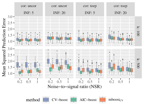
Figure 6: Mean Squared Prediction Error for new variable selection strategies by simulation setting.

A.2 Simulation Results of Poisson Distributed Data

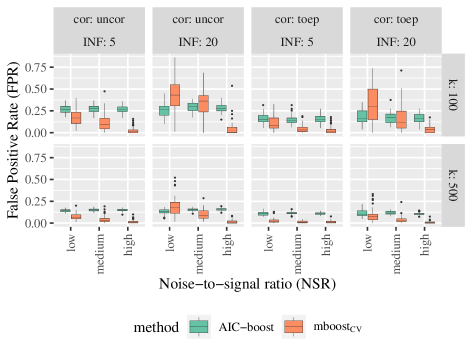
Figure 9: False Positive Rate for new variable selection strategies by simulation setting.

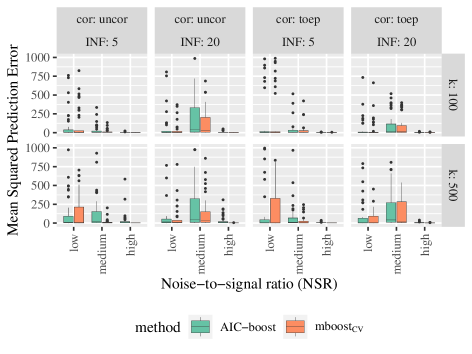
Figure 10: Mean Squared Prediction Error for new variable selection strategies by simulation setting.

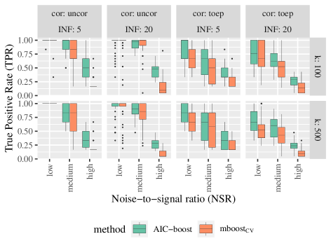
Figure 11: True Positive Rate for new variable selection strategies by simulation setting.

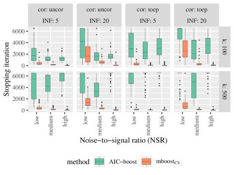
Figure 12: Stopping iteration $t^{*}$ for new variable selection strategies by simulation setting.

Appendix B Application Results

B.1 Model Table of Application

Table 6: Coefficients of standardized covariates on log(age-standardized incidence rate) of different estimation models. Numbers in brackets correspond to the ordering of the absolute values of the coefficients.

Covariate	$\text{mboost}_{\text{CV}}$		LASSO		AIC-boost
Intercept	$4.133$		$3.992$		$2.829$
Age-standardized incidence rate per 100.000 person-years until 15.03.	$0.043$	(5)	$0.046$	(6)	$0.109$	(6)
Unemployment rate of young persons (under 26 years) in 2017	$-0.071$	(4)	$-0.055$	(5)	$-0.071$	(8)
%Voter turnout (Number of valid votes in the last Bundestag election) of all registered voters	$0.023$	(7)	$0.036$	(7)	$0.033$	(13)
%Roman-catholics in 2011	$0.075$	(3)	$0.079$	(4)	$0.086$	(7)
Persons in long-term care per 10.000 persons in 2017	$-0.024$	(6)	$-0.033$	(8)	$-0.039$	(12)
Premature mortality (deaths of persons younger than 65 years) per 1,000 persons	$-0.097$	(2)	$-0.088$	(3)	$-0.117$	(5)
%Households with low income (1,500€ per month) in all households in 2016	$-0.015$	(8)	$-0.015$	(9)	$-0.012$	(18)
Latitude	$-0.122$	(1)	$-0.130$	(2)	$-0.130$	(4)
%Older employed persons (55 years+) in all employed persons in 2017			$-0.013$	(10)
Ever 100+ inbound commuters from Tirschenreuth			$0.141$	(1)	$0.920$	(1)
%Change of number of persons at age 50-65 in 2012-2017					$0.009$	(19)
Sex ratio (females to males) at age 20-40 in 2017					$0.021$	(17)
Total sex ratio (females to males) in 2017					$0.068$	(9)
%Young employed persons in all young persons (under 26 years) in 2017					$0.054$	(11)
%Older employed persons in all older persons (55 years+) in 2011-2017					$0.027$	(15)
%Change of number of employed persons in 2012-2016					$0.009$	(19)
Average travel time to the next large-sized regional center ("Oberzentrum")					$-0.032$	(14)
%Outbound commuters over a distance of 50km+ in all employed persons in 2017					$-0.006$	(20)
%Outbound commuters over a distance of 150km+ in all employed persons in 2017					$-0.056$	(10)
Ever 100+ inbound commuters from Hohenlohekreis					$0.136$	(3)
Ever 100+ inbound commuters from Aachen					$0.027$	(15)
Ever 100+ inbound commuters from Rosenheim (city + district)					$0.194$	(2)

References

- [1] Peter Bühlmann and Torsten Hothorn. Boosting Algorithms: Regularization, Prediction and Model Fitting. Statistical Science, 22(4):477–505, 2007.
- [2] Yoav Freund and Robert E Schapire. Experiments with a new boosting algorithm. Proceedings of the Thirteenth International Conference on Machine Learning Theory, pages 148–156, 1996.
- [3] Leo Breiman. Arcing the edge. Technical report, 486, Statistics Department, University of California at Berkeley, 1997.
- [4] Jerome Friedman, Trevor Hastie, and Robert Tibshirani. Additive logistic regression: a statistical view of boosting (with discussion and a rejoinder by the authors). The Annals of Statistics, 28(2):337–407, 2000.
- [5] Jerome Friedman. Greedy function approximation: A gradient boosting machine. The Annals of Statistics, 29(5):1189–1232, 2001.
- [6] Andreas Mayr, Benjamin Hofner, and Matthias Schmid. The Importance of Knowing When to Stop. Methods of Information in Medicine, 51(02):178–186, 2012.
- [7] Janek Thomas, Tobias Hepp, Andreas Mayr, Bernd Bischl, and Yuhai Zhao. Probing for Sparse and Fast Variable Selection with Model-Based Boosting. Computational and Mathematical Methods in Medicine, 2017:1–8, 2017.
- [8] Nicolai Meinshausen and Peter Bühlmann. Stability selection. Journal of the Royal Statistical Society: Series B (Statistical Methodology), 72(4):417–473, 2010.
- [9] Benjamin Hofner, Luigi Boccuto, and Markus Göker. Controlling false discoveries in high-dimensional situations: Boosting with stability selection. BMC bioinformatics, 16(1):1–17, 2015.
- [10] Annika Strömer, Christian Staerk, Nadja Klein, Leonie Weinhold, Stephanie Titze, and Andreas Mayr. Deselection of base-learners for statistical boosting—with an application to distributional regression. Statistical Methods in Medical Research, 31(2):207–224, 2022.
- [11] Peter Bühlmann and Torsten Hothorn. Twin boosting: improved feature selection and prediction. Statistics and Computing, 20(2):119–138, 2010.
- [12] Christian Staerk and Andreas Mayr. Randomized boosting with multivariable base-learners for high-dimensional variable selection and prediction. BMC bioinformatics, 22(1):1–28, 2021.
- [13] Peter Bühlmann, Bin Yu, Yoram Singer, and Larry Wasserman. Sparse boosting. Journal of Machine Learning Research, 7(6):1001–1024, 2006.
- [14] Benjamin Hofner, Torsten Hothorn, Thomas Kneib, and Matthias Schmid. A Framework for Unbiased Model Selection Based on Boosting. Journal of Computational and Graphical Statistics, 20(4):956–971, 2011.
- [15] Gerhard Tutz and Andreas Groll. Generalized Linear Mixed Models Based on Boosting. Statistical Modelling and Regression Structures: Festschrift in Honour of Ludwig Fahrmeir, pages 197–215, 2010.
- [16] Ludwig Fahrmeir, Thomas Kneib, Stefan Lang, and Brian D. Marx. Generalized linear models. Regression Models, pages 283–342, 2021.
- [17] Trevor Hastie. Comment: Boosting Algorithms: Regularization, Prediction and Model Fitting. Statistical Science, 22(4):513–515, November 2007.
- [18] Torsten Hothorn, Peter Bühlmann, Thomas Kneib, Matthias Schmid, and Benjamin Hofner. Model-based Boosting 2.0. Journal of Machine Learning Research, 11(71):2109–2113, 2010.
- [19] Tobias Hepp, Matthias Schmid, Olaf Gefeller, Elisabeth Waldmann, and Andreas Mayr. Approaches to Regularized Regression - A Comparison between Gradient Boosting and the Lasso. Methods of Information in Medicine, 55(5):422–430, 2016.
- [20] Gabriele Doblhammer, Constantin Reinke, and Daniel Kreft. Social disparities in the first wave of COVID-19 incidence rates in Germany: a county-scale explainable machine learning approach. BMJ Open, 12(2: e049852):1–11, February 2022.
- [21] Thomas Plümper and Eric Neumayer. The pandemic predominantly hits poor neighbourhoods? SARS-CoV-2 infections and COVID-19 fatalities in German districts. European journal of public health, 30(6):1176–1180, 2020.
- [22] Benjamin Wachtler, Niels Michalski, Enno Nowossadeck, Michaela Diercke, Morten Wahrendorf, Claudia Santos-Hövener, Thomas Lampert, and Jens Hoebel. Socioeconomic inequalities in the risk of SARS-CoV-2 infection - First results from an analysis of surveillance data from Germany. Journal of health monitoring, 5(Suppl 7):18–29, 2020.
- [23] Sven Rohleder, Diogo Costa, and Kayvan Bozorgmehr. Area-level socioeconomic deprivation, non-national residency, and Covid-19 incidence: A longitudinal spatiotemporal analysis in Germany. EClinicalMedicine, 49:101485, 2022.
- [24] Thomas Plümper, Denise Laroze, and Eric Neumayer. The limits to equivalent living conditions: regional disparities in premature mortality in Germany. Journal of public health, 26(3):309–319, 2018.
- [25] M. Brandl, R. Selb, S. Seidl-Pillmeier, D. Marosevic, U. Buchholz, and S. Rehmet. Mass gathering events and undetected transmission of SARS-CoV-2 in vulnerable populations leading to an outbreak with high case fatality ratio in the district of Tirschenreuth, Germany. Epidemiology and infection, 148:e252, 2020.
- [26] Clemens Fuest and Lea Immel. Ein zunehmend gespaltenes Land? – Regionale Einkommensunterschiede und die Entwicklung des Gefälles zwischen Stadt und Land sowie West- und Ostdeutschland. ifo Schnelldienst, 72(16):19–28, 2019.
- [27] Aranka Viviënne Ballering, Sabine Oertelt-Prigione, Tim C. Olde Hartman, and Judith G. M. Rosmalen. Sex and Gender-Related Differences in COVID-19 Diagnoses and SARS-CoV-2 Testing Practices During the First Wave of the Pandemic: The Dutch Lifelines COVID-19 Cohort Study. Journal of women’s health, 30(12):1686–1692, 2021.
- [28] Vanessa Bianconi, Massimo R. Mannarino, Paola Bronzo, Ettore Marini, and Matteo Pirro. Time-related changes in sex distribution of COVID-19 incidence proportion in Italy. Heliyon, 6(10):e05304, 2020.
- [29] Achim Doerre and Gabriele Doblhammer. The influence of gender on COVID-19 infections and mortality in Germany: Insights from age- and gender-specific modeling of contact rates, infections, and deaths in the early phase of the pandemic. PloS one, 17(5):e0268119, 2022.
- [30] Julio Ancochea, Jose L. Izquierdo, and Joan B. Soriano. Evidence of Gender Differences in the Diagnosis and Management of Coronavirus Disease 2019 Patients: An Analysis of Electronic Health Records Using Natural Language Processing and Machine Learning. Journal of women’s health, 30(3):393–404, 2021.
- [31] Tim Leibert, Manuel Wolff, and Annegret Haase. Shifting spatial patterns in German population trends: local-level hot and cold spots, 1990–2019. Geographica Helvetica, 77(3):369–387, 2022.
- [32] Philipp Fink, Martin Hennicke, and Heinrich Tiemann. Unequal Germany: Socio-economic disparities report 2019. For a better tomorrow. Friedrich-Ebert-Stiftung, Bonn, 2019.
- [33] W. S. Robinson. Ecological Correlations and the Behavior of Individuals. American Sociological Review, 15(3):351–357, June 1950.
- [34] Clifford M Hurvich and Chih-Ling Tsai. Regression and time series model selection in small samples. Biometrika, 76(2):297–307, 1989.
- [35] Peter Bühlmann and Torsten Hothorn. Rejoinder: Boosting Algorithms: Regularization, Prediction and Model Fitting. Statistical Science, 22(4):516–522, 2007.