Key-Exchange Convolutional Auto-Encoder for Data Augmentation in Early Knee OsteoArthritis Classification

Abstract

Knee OsteoArthritis (KOA) is a prevalent musculoskeletal condition that impairs the mobility of senior citizens. The lack of sufficient data in the medical field is always a challenge for training a learning model due to the high cost of labelling. At present, Deep neural network training strongly depends on data augmentation to improve the model’s generalization capability and avoid over-fitting. However, existing data augmentation operations, such as rotation, gamma correction, etc., are designed based on the original data, which does not substantially increase the data diversity. In this paper, we propose a learning model based on the convolutional Auto-Encoder and a hybrid loss strategy to generate new data for early KOA (KL-0 vs KL-2) diagnosis. Four hidden layers are designed among the encoder and decoder, which represent the key and unrelated features of each input, respectively. Then, two key feature vectors are exchanged to obtain the generated images. To do this, a hybrid loss function is derived using different loss functions with optimized weights to supervise the reconstruction and key-exchange learning. Experimental results show that the generated data are valid as they can significantly improve the model’s classification performance.

Keywords Auto-Encoder  $\cdot$ Key feature  $\cdot$ Data augmentation  $\cdot$ Knee osteoarthritis

1 Introduction

Knee OsteoArthritis (KOA) is a degenerative illness characterized by articular cartilage deterioration and damage, joint edges, and subchondral bone reactive hyperplasia [1]. Multiple factors, including age, weight, stress, trauma, etc. [2], may contribute to its occurrence. Patients may experience excruciating pain and restricted mobility, which can significantly impact their quality of life and increase their risk for chronic diseases such as cardiovascular disease [3]. According to United Nations figures, by 2050, those over 60 will constitute more than 20$\%$ of the global population [4]. Unfortunately, the aetiology of KOA is presently unknown, and there is no cure [5]. Therefore, early detection of KOA is essential so that timely behavioural therapies, such as weight loss, can be implemented to postpone the onset and progression of KOA [6].

In 1957, Kellgren and Lawrence first proposed the Kellgren-Lawrence (KL) grading system [7] for KOA. As can be seen in Table 1, KOA can be divided into five grades based on the existence and severity of symptoms such as osteophytes and Joint Space Narrowing (JSN). The KL grading system is a semi-quantitative criterion for evaluating the severity of KOA, despite being a widely used grading system. The diagnosis of KOA based on KL features depends entirely on the practitioners’ experience and subjectivity, medical professionals may therefore assign varying grades to the same knee X-ray image [8].

Table 1: Description of the KL grading system

Grade	Severity	Description
KL-0	none	definite absence of osteoarthritis
KL-1	doubtful	possible osteophytic lipping
KL-2	minimal	definite osteophytes and possible JSN
KL-3	moderate	moderate multiple osteophytes, definite JSN, some
		sclerosis and possible deformity of bone ends
KL-4	severe	large osteophytes, definite JSN, severe sclerosis and
		definite bone ends deformity.

Deep learning, a fundamental component of artificial intelligence, has gained traction in the field of computer vision in recent years, particularly the use of Convolutional Neural Networks (CNNs) [9], which have effectively accomplished tasks such as detection [10], segmentation [11] and classification [12].

Figure 1: The flowchart of the proposed KECAE model. Black, blue, and red arrows represent the overall dataflow, unrelated and key features, respectively. $\oplus$ represents the bit-wise addition.

For KOA classification, several deep-learning models have been developed. In [13], Antony et al. employed the Fully Convolutional Neural (FCN) network [14] to locate the knee joint automatically and classify full KL grades using the classical CNN. In [15], Tiuplin et al. cropped two patches from the lateral and medial parts of the knee joint X-ray images as the input pair of the Siamese network to evaluate the KOA grade. In [16], to improve the classification performance of early KOA (KL-0 vs KL-2), Wang et al. integrated a collection of Global Average Pooling (GAP) layers at each level of the Siamese network for the feature fusion. Although the models proposed in different approaches have their own characteristics and successes, the decision-making process is widely regarded as a black box. Therefore, in [15] and [16], the Grad-CAM [17] technique was used to visualize attention maps and thus enhance the interpretability of the models.

In the field of deep learning for medical images, the small quantity of valid medical datasets is always a big challenge for training the learning model due to the high cost of labelling [18]. At present, the training of deep neural networks relies heavily on data augmentation to improve the model’s generalization ability and avoid over-fitting [19]. However, traditional data augmentation methods, such as rotation, gamma correction, etc., are designed on the original data, which does not change the data structure of the samples and thus does not substantially increase the diversity of samples. Therefore, several approaches based on the Generative Adversarial Network (GAN) [20] were proposed to generate new data as an efficient and straightforward approach to data augmentation. In [21], Tanaka et al. proved that the generation of artificial training data is useful for handling dataset imbalance. Their proposed GAN-based model was evaluated on benchmark datasets using different models. Experimental results showed that a Decision Tree (DT) classifier [22] trained using data generated by the GAN model achieved the same performance as a DT trained on the original dataset. In [23], Frid-Adar et al. used DCGAN [24] to synthesize different classes of lesion plaques from liver CT and trained an independent generative model for each category: cysts, metastases and hemangiomas. The authors showed that synthetic samples from DCGAN can improve the performance of CNN classifiers.

However, the texture details in the generated images via GAN-based models do not fully meet the high standard of quality needed in medical diagnosis, especially for tasks requiring fine texture details, such as early diagnosis of KOA. The difficulty of the GAN’s convergence makes it hard for the model to reach the Nash equilibrium [25]. Consequently, the experimental results are challenging to reproduce. Moreover, until now, no meaningful indicator has been associated with the quality of the generated images.

Considering that KOA is definitely present at KL-2, compared to doubtful KL-1, the labels of KL-2 data have higher confidence. Therefore, the early prediction of KL-2 has greater clinical value. Taking this into consideration, in this paper, we propose a novel model based on the Convolutional Auto-Encoder (CAE) to generate new X-ray data as a data augmentation method for the early KOA classification (i.e., KL-0 vs KL-2). Our proposed method is inspired by GAN and the work of [26] and [27]. Compared to the classic AE model, the encoder in our proposed model takes a dual simultaneous input of two images (one is KL-0, and the other is KL-2) and produces two hidden vectors (one is the key feature vector, and the other is the unrelated feature vector) for each image. These two pairs of vectors are added bit-wise to produce two hidden vectors that are then passed through the decoder to obtain corresponding reconstructed outputs. Simultaneously, the key feature vector of each image is exchanged in order to perform a bit-wise summation with the unrelated vector from the other input. These two resulting vectors are then passed through the decoder to obtain corresponding key-exchanged outputs. To do so, a hybrid loss function is proposed, which consists of the Mean Square Error (MSE) loss, the Cross-Entropy (CE) loss, and the Fisher Linear Discriminant Analysis (LDA) algorithm [28][29] as a loss distance. The final loss is derived by combining the above loss functions along with optimized weights. Finally, the generated key-exchanged outputs are used to expand the original dataset to improve the classifier performance.

The main contributions of this paper are as follows:

• A Key-Exchange Convolutional Auto-Encoder (KE-CAE) learning model is proposed to generate new data for early KOA diagnosis (i.e., KL-0 vs KL-2) as a data augmentation method.

• Key and unrelated feature vectors are visualized to clearly show the principle of generating key-exchanged outputs.

• Experimental data were obtained from the OsteoArthritis Initiative (OAI) [30] database.

2 Proposed Approach

Before describing the proposed architecture, we briefly present the classical Auto-Encoder (AE) model [31]. For greater convenience, the important symbols used in this paper are introduced in Table 2.

Table 2: Important symbols used in this paper

Symbol	Description
$\mathcal{K}$	a set of KL grades (KL-0 and KL-2)
$\mathcal{T}$	the training set
$\hat{Y}$	the predicted labels
$Y$	the real labels

2.1 Classical Auto-Encoder network

Figure 2: The structure of the classical AE network[31].

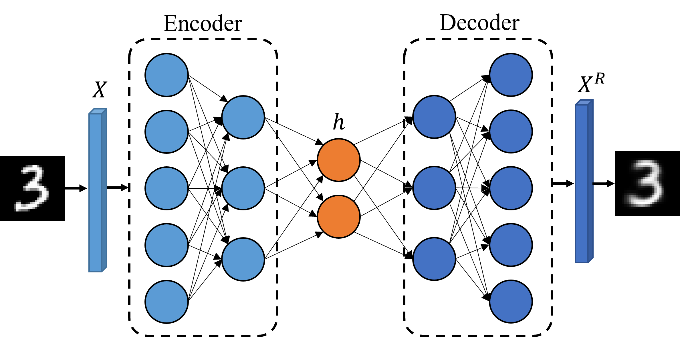
As shown in Fig. 2, AE is an unsupervised learning model that consists of an encoder and a decoder. It uses the input data $X$ itself as supervision to make the neural network learn a mapping relationship, and thereby obtains a reconstructed output $\hat{X}$. More precisely, the encoder aims to encode the high-dimensional input $X$ into a low-dimensional hidden variable $h$ so that the neural network learns the most informative features. The decoder restores the hidden variable $h$ of the hidden layer to the original dimension, and the goal of the model is to make its output a faithful approximate of the input (i.e., $minimize(dist(\hat{X},X))$).

The encoding process of the original data $X$ from the input to the hidden layers is as follows:

$$h=g_{\theta_{1}}(X)=\sigma(W_{1}X+b_{1})$$ (1)

where $g_{\theta_{1}}$ is the function of the encoder, $\sigma$ is an activate function, $W_{1}$ and $b_{1}$ are weight and bias matrices of the encoder, respectively.

The decoding process of the hidden variable $h$ from the hidden layer to the output layer is as follows:

$$\hat{X}=g_{\theta_{2}}(h)=\sigma(W_{2}h+b_{2})$$ (2)

where $g_{\theta_{2}}$ is the function of the decoder, $W_{2}$ and $b_{2}$ are the weight and the bias matrices of the decoder, respectively.

Usually, the AE model minimizes the reconstruction error using the Mean Square Error (MSE) cost function, which is defined as:

$$J_{MSE}=\frac{1}{N}\sum_{i=1}^{N}(\hat{X}-X)^{2},\quad{\forall}X\in\mathcal{T}$$ (3)

where $N$ is the number of samples in each training batch. $\mathcal{T}$ represents the training set.

Compared to Principal Components Analysis (PCA) [32], the AE model can achieve non-linear dimensionality reduction of the data. The main advantage of the AE network is that it has a strong generalization capability and does not require data annotation.

2.2 Proposed learning model

Despite the fact that the basic goal of the classical AE network is to reconstruct the input, it can also be used to extract features. For instance, Nasser et al. [26] used five ROIs cropped from the tibial plateau as the inputs of the AE to obtain the corresponding feature vectors, and then fed them to different classifiers to evaluate the respective KOA classification performance.

Algorithm 1 Learning algorithm of the proposed approach

Input: $X_{1},X_{2}$, and all initial parameters
      Output: $\hat{X_{1}},\hat{X_{2}},X_{1}^{\prime},X_{2}^{\prime}$, and learned parameters
      repeat
            Compute $J_{CE}(X_{1}),J_{CE}(X_{2})$ $\triangleright$ Eq. 5
            Update Parameters of the discriminator
            Freeze Parameters of the discriminator
            Get $h_{1}^{U},h_{1}^{K};h_{2}^{K},h_{2}^{U}\leftarrow encoder(X_{1},X_{2})$
            Get $h_{1}\leftarrow h_{1}^{U}\oplus h_{1}^{K}$, $h_{2}\leftarrow h_{2}^{U}\oplus h_{2}^{K}$
            Get $\hat{X_{1}},\hat{X_{2}}\leftarrow decoder(h_{1},h_{2})$
            Compute $J_{MSE}(X_{1},\hat{X_{1}})$, $J_{MSE}(X_{2},\hat{X_{2}})$ $\triangleright$ Eq. 3
            Exchange $h_{1}^{K}$ $\leftrightarrows$ $h_{2}^{K}$
            Get $h_{1}^{\prime}\leftarrow h_{1}^{U}\oplus h_{2}^{K}$, $h_{2}^{\prime}\leftarrow h_{2}^{U}\oplus h_{1}^{K}$
            Get $X_{1}^{\prime},X_{2}^{\prime}\leftarrow decoder(h_{1}^{\prime},h_{2}^{\prime})$
            Compute $J_{CE}(X_{1}^{\prime})$, $J_{CE}(X_{2}^{\prime})$ $\triangleright$ Eq. 5
            Compute $J_{LDA}(h_{1}^{U},h_{1}^{K})$, $J_{LDA}(h_{2}^{U},h_{2}^{K})$ $\triangleright$ Eq. 10
            Update Parameters of the encoder and decoder
            Unfreeze Parameters of the discriminator
      until convergence

Inspired by this, we propose here the Key-Exchange Convolutional Auto-Encoder (KE-CAE). As presented in Fig. 1, our proposed model consists of three main modules: an encoder, a decoder, and a discriminator. Compared to the classic AE model, two inputs (i.e., $X_{1}$ and $X_{2}$) and four hidden vectors (i.e., $h_{1}^{U}$, $h_{1}^{K}$, $h_{2}^{U}$, and $h_{2}^{K}$) were designed. $h^{U}$ and $h^{K}$ represent the unrelated and key feature vectors, respectively. More precisely, the proposed encoder takes a dual simultaneous input of two images ($X_{1}$ and $X_{2}$) and produces two pairs of hidden vectors ($h_{1}^{K}$ and $h_{1}^{U}$, $h_{2}^{K}$ and $h_{2}^{U}$) for each input. They are then added bit-wise to produce two hidden vectors ($h_{1}$ and $h_{2}$) that are then passed through the decoder to obtain the corresponding reconstructed outputs ($\hat{X_{1}}$ and $\hat{X_{2}}$). Simultaneously, the key feature vector $h^{K}$ of each input is exchanged, and a bit-wise summation with the unrelated vector $h^{U}$ from the other input is performed. The resulting two vectors ($h_{1}^{\prime}$ and $h_{2}^{\prime}$) are passed through the decoder to obtain two key-exchanged outputs ($X_{1}^{\prime}$ and $X_{2}^{\prime}$).

To achieve feature extraction between the key and unrelated feature vectors, we used the Siamese-GAP network [16], which achieved the best performance on the classification of early KOA (KL-0 and KL-2), as a discriminator and also a supervisor. First, the discriminator is trained using the two inputs ($X_{1}$ and $X_{2}$) to learn the discriminatory features. Then, the parameters of the discriminator are frozen. After this, the discriminator supervises two key-exchanged outputs ($X_{1}^{\prime}$ and $X_{2}^{\prime}$). Finally, four outputs ($\hat{X_{1}}$, $X_{1}^{\prime}$, $\hat{X_{2}}$, and $X_{2}^{\prime}$) are obtained via the proposed KE-CAE model. It is noteworthy that the labels of these two key-exchanged outputs are also exchanged. Algorithm 1 describes the training process of the proposed approach.

Figure 3: Structures of the encoder (a) and the decoder (b) of the proposed KE-CAE model.

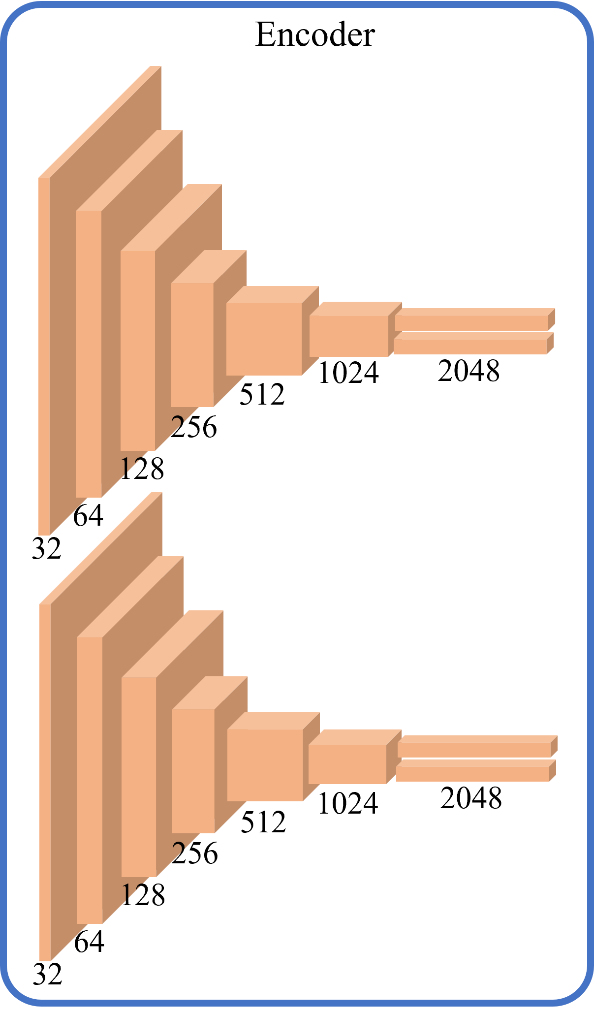
The structures of our encoder and decoder modules are shown in Fig.3. The encoder is based on two identical CNNs with shared parameters, where each CNN has 20 layers divided into seven blocks. Each block consists of a set of convolution layers of the same kernel of size 3$\times$3 with different depths (i.e., 32, 64, 128, 256, 512, 1024 and 2048) - a Batch Normalization (BN) layer - Leaky Rectified Linear Unit (LeakyReLU) layer with a predefined slope of 0.2. The structures of the encoder and the decoder are almost symmetrical. The decoder consists of seven DeConvolutional Neuron Network (DCNN) blocks. These blocks consist of a set of deconvolutional layers of the same kernel size of 4$\times$4 with different depths (i.e., 2048, 1024, 512, 256, 128, 64, 32, and 1) - a BN layer - a LeakyReLU layer with a predefined slope of 0.2.

2.3 Hybrid loss strategy

As presented in Section 2.1, MSE (Eq. 3) is usually used as a reconstruction loss function. In this study, as there are two reconstruction outputs $\hat{X_{1}}$ and $\hat{X_{2}}$, two MSE losses $J_{MSE}(X_{1},\hat{X_{1}})$ and $J_{MSE}(X_{2},\hat{X_{2}})$ are thus obtained. Therefore, we defined the $J_{MSE}$ as follows:

$$J_{MSE}=J_{MSE}(X_{1},\hat{X_{1}})+J_{MSE}(X_{2},\hat{X_{2}})$$ (4)

The discriminator is used to learn the discriminatory features from the original images $X_{1}$ and $X_{2}$, and also to supervise the two key-exchanged outputs $X_{1}^{\prime}$ and $X_{2}^{\prime}$ using the CE loss, called here $J_{CE}$, which is computed as follows:

$$J_{CE}=\frac{1}{N}\sum_{s\in\mathcal{T}}-\left[y_{s}log(p_{s})+(1-y_{s})log(1-p_{s})\right]$$ (5)

$$y_{s}=\left\{\begin{array}[]{lcr}1,&&{\hat{Y}=T}\\ 0,&&{\hat{Y}\neq T}\\ \end{array}\right.$$ (6)

$$p_{s}=P_{\hat{Y}|T}(\hat{Y}=k|T=k),\quad{\forall}k\in\mathcal{K}$$ (7)

where $y_{s}$ is the one-hot encoded ground-truth label of the sample $s$. $N$ is the number of the sample $s$. $\hat{Y}$ and $T$ are the predicted and the real labels, respectively. $k$ represents the KL grade of the sample $s$, $P_{\hat{Y}|T}$ is the conditional probability distribution and $\mathcal{K}$ is a set of KL grades $\left\{KL-0,KL-2\right\}$.

During the discriminator active learning, two CE losses $J_{CE}(X_{1})$ and $J_{CE}(X_{2})$ are obtained. Therefore, the discriminator learning loss, namely $J_{CE_{1}}$, is defined as:

$$J_{CE_{1}}=J_{CE}(X_{1})+J_{CE}(X_{2})$$ (8)

As presented in Section 2, two key-exchanged outputs $X_{1}^{\prime}$ and $X_{2}^{\prime}$ are supervised by the discriminator, and thus the classification losses $J_{CE}(X_{1}^{\prime})$ and $J_{CE}(X_{2}^{\prime})$ are obtained, respectively. Therefore, the supervised loss function $J_{CE_{2}}$ is defined here by:

$$J_{CE_{2}}=J_{CE}(X_{1}^{\prime})+J_{CE}(X_{2}^{\prime})$$ (9)

To separate the key and unrelated features from the corresponding original image, we used the LDA algorithm, which is a supervised learning technique for dimensionality reduction and projects the high-dimensional sample data into the vector space to maximize the inter-class distance and minimize the intra-class distance in the new subspace. It is computed as follows:

$$J_{LDA}=\frac{({\sigma^{U}})^{2}+({\sigma^{K}})^{2}}{\left|\mu^{U}-\mu^{K}\right|^{2}}$$ (10)

$$\mu^{i}=\frac{1}{N}\sum_{n=1}^{N}x_{n},\quad(\sigma^{i})^{2}=\frac{1}{N}\sum_{n=1}^{N}(x_{n}-\mu^{i})^{2}$$ (11)

where $\mu^{i}$, $(\sigma^{i})^{2}$, $N$ denote the mean, variance, and number of elements ($x_{1}$, …, $x_{n}$) in the feature vector, respectively. $i$ $\in$ $\left\{U,K\right\}$ represents the unrelated $U$ and key feature $K$ vectors.

Finally, the proposed hybrid loss function is defined as:

$$J_{KE-CAE}=J_{MSE}+J_{CE_{1}}+\lambda_{1}J_{CE_{2}}+\lambda_{2}J_{LDA}$$ (12)

where the hyper-parameters $\lambda_{1}$ and $\lambda_{2}$ are used to weigh and better balance the above loss functions. Their effects on the performance will be discussed in Section 4.1.

3 Experimental settings

In this section, experimental data and details are presented.

3.1 Public Knee Datasets

In this study, a freely-accessible database, OsteoArthritis Initiative (OAI) [30], was used. The OAI is a longitudinal research that includes nine follow-up assessments of 4,796 participants over 96 months. Participants range in age from 45 to 79 years. The OAI seeks to enrol participants with KOA or a high risk of developing it.

3.2 Data preprocessing

Figure 4: Original knee radiography and the ROI obtained in red (a), patches extracted in blue and orange boxes (b), resulting patches as the input for the discriminator (c).

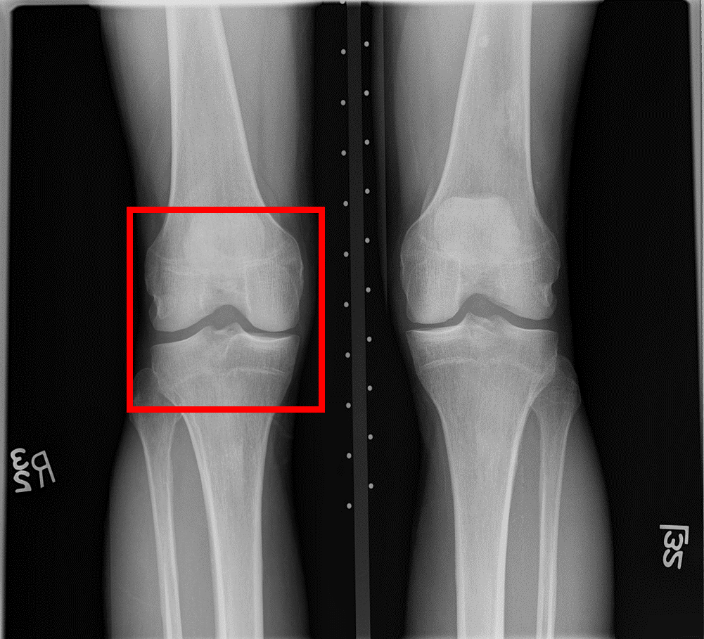
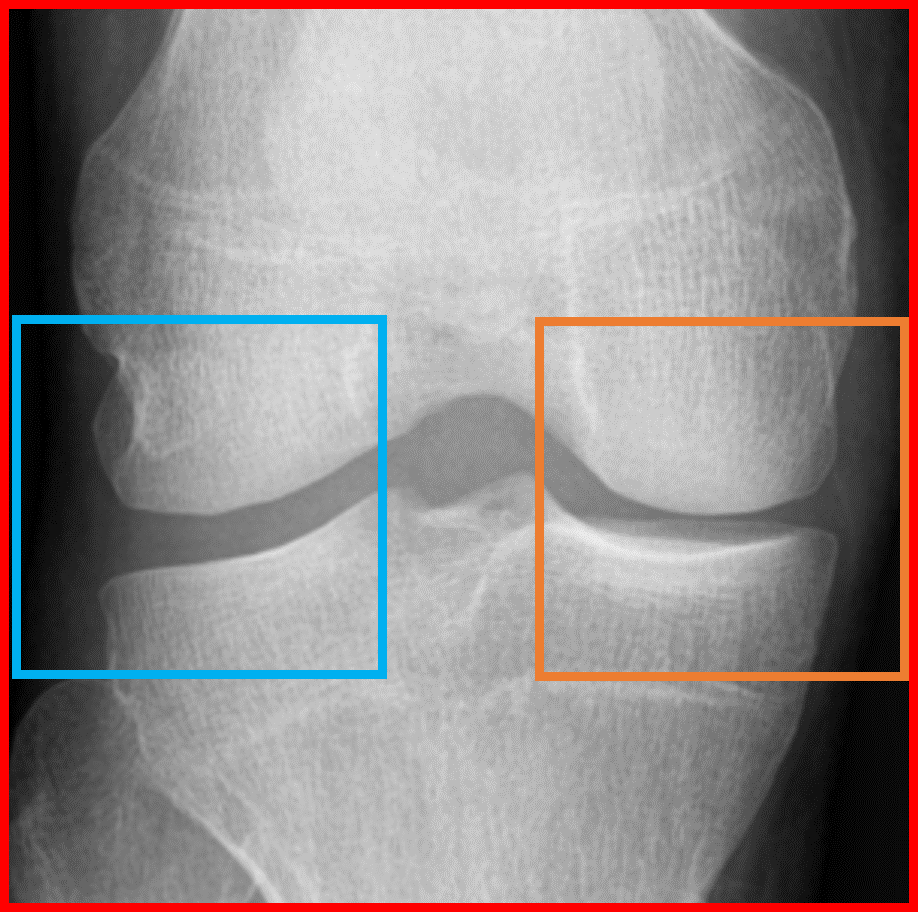
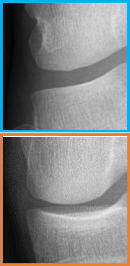
The ROIs used in [33] and extracted using YOLOv2 (Fig. 4) were employed as inputs of the encoder module. For the discriminator, as the objective of this study was for early KOA classification (KL-0 vs KL-2), we explored the features of the lateral and medial sides of the knee joint. To do this, the completely automated segmentation method used in [15] was employed to obtain two patches (Fig. 4) covering the whole distal area (osteophytes and JSN). More specifically, two 128$\times$128-pixel-square patches were extracted from the left and right one-third parts of the knee joint. Then, the medial side patch was flipped horizontally. Finally, as shown in Fig. 4, two patches were obtained and used as inputs for the discriminator.

After these preprocessing procedures, 3,185 and 2,126 knee X-rays of KL-0 and KL-2 were retained, respectively. Then, bootstrapping-based oversampling [34] was thus applied for the KL-2 set. After this, the overall data were randomly partitioned into training, validation and test subsets according to each KL grade with a ratio of 7:1:2. As the labels of the two inputs ($X_{1}$ and $X_{2}$) have to be different, here we used the global permutation strategy on the training set: each KL-0 image was combined with all KL-2 images in turn to form different input pairs. As a result, a total of 3,455,881 input pairs was obtained. To simplify this and save computational resources, we took a random sample of 50,000, 100,000, 500,000, and 1,000,000 from the total input pairs, which will be discussed in Section 4.3.

3.3 Experimental details

The weights of all modules (encoder, decoder, and discriminator) were initialized using the Kaiming procedure [35]. Adam optimizer method was employed for training with 1,000 epochs, a mini-batch size of 30 and a learning rate of 1e-04 for the encoder and decoder, and of 1e-05 for the discriminator. The parameters of the discriminator were frozen during the supervising process. Common data augmentation techniques, such as random rotation, brightness, contrast, etc., were executed randomly during the training of the discriminator. Our approach was implemented using PyTorch v1.8.1 [36] on Nvidia TESLA A100 - 40 GB memory graphic cards.

4 Results and discussion

In this section, experimental results are presented and discussed.

4.1 Selection of the hyper-parameters

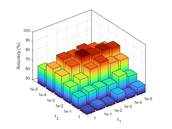
The hyper-parameters $\lambda_{1}$ and $\lambda_{2}$ of the proposed hybrid loss strategy were tuned via a small grid search over combinations of $\lambda_{1},\lambda_{2}\in[1e^{-5},1]$. To evaluate more intuitively the capability of the key feature extraction of the model, Fig. 5 illustrates the classification accuracy depending on $\lambda_{1}$ and $\lambda_{2}$ using the Support Vector Machine with the Radial Basis Function (SVM-RBF) [37] for the key feature vector $h^{K}$. As can be seen, compared to $\lambda_{1}$, $\lambda_{2}$ is more sensitive to accuracy. If the value of $\lambda_{2}$ is set too large (i.e., between 1e-01 and 1), feature separation is almost ineffective, regardless of the value of $\lambda_{1}$. When $\lambda_{2}$ is set between 1e-05 and 1e-02, the accuracy fluctuates as $\lambda_{1}$ changes. Of these, the best classification performance was achieved with $\lambda_{1}=1e^{-2}$ and $\lambda_{2}=1e^{-3}$, which were retained for the following experiments.

Figure 5: Performance obtained using SVM-RBF with different values of $\lambda_{1}$ and $\lambda_{2}$ for $h^{K}$.

4.2 Visualization of the feature vectors

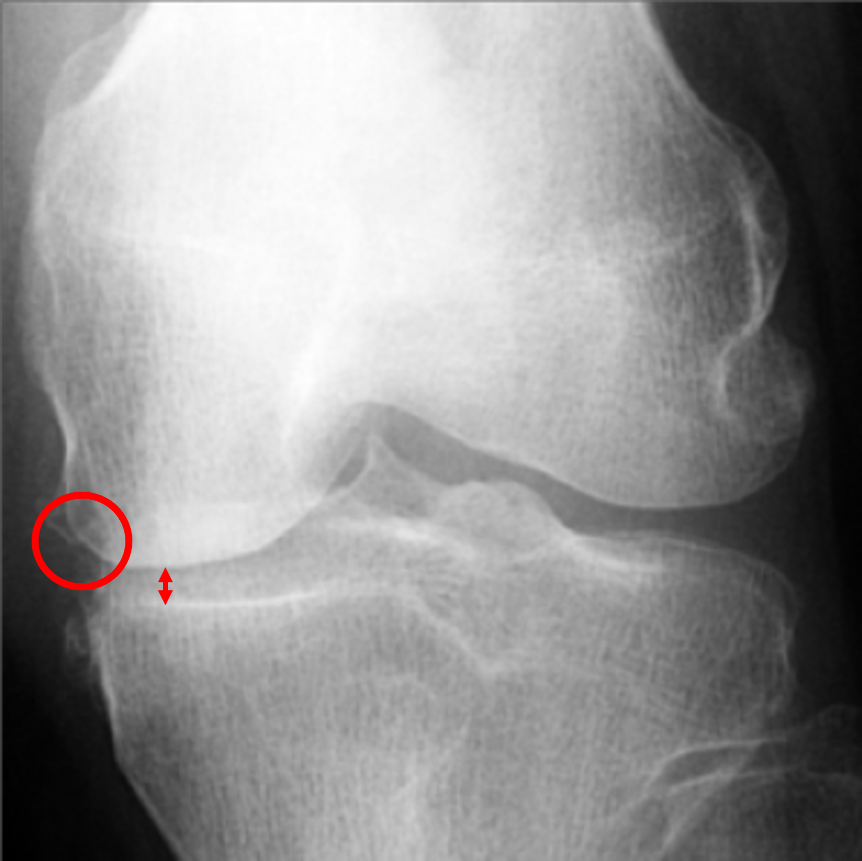
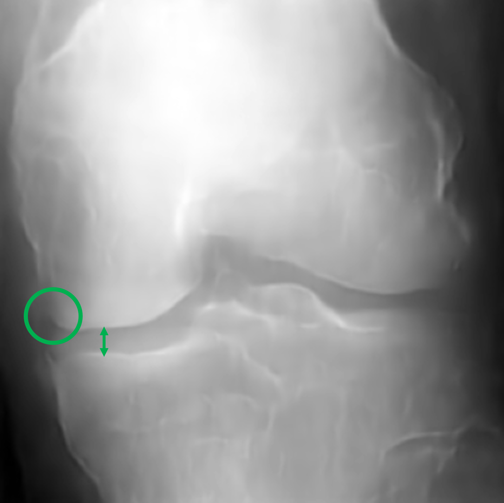
In this section, we analyzed the key parts of our approach through 2D illustrations of the results obtained. In Table 3, we show the original input pair ($X_{1}$ and $X_{2}$), the extracted feature vectors ($h_{1}^{K}$, $h_{1}^{U}$, $h_{2}^{K}$, and $h_{2}^{U}$), the reconstructed outputs ($\hat{X}_{1}$ and $\hat{X}_{2}$), and exchanged outputs ($X^{\prime}_{1}$ and $X^{\prime}_{2}$). As can be seen, the key and unrelated feature vectors ($h^{K}$ and $h^{U}$) clearly show the feature separation. Compared to $h^{U}$, $h^{K}$ always focuses on the area of symptoms of early KOA (i.e., joint space and osteophytes). Reconstructed outputs ($\hat{X}_{1}$ and $\hat{X}_{2}$) show the model’s efficient reconstruction performance. Key-exchanged outputs ($X_{1}^{\prime}$ and $X_{2}^{\prime}$) indicate that several symptoms based on their original background contour were incorporated or removed from the reconstructed images. For better clarity, Fig. 6 highlights the differences between $X_{1}$ (Fig. 6(a)) and $X_{1}^{\prime}$ (Fig. 6(b)) as well as between $X_{2}$ (Fig. 6(c)) and $X_{2}^{\prime}$ (Fig. 6(d)). As can be seen, for $X^{\prime}_{1}$, the symptoms of KL-2 (i.e., JSN and a few osteophytes) were added to the KL-0 healthy knee $X_{1}$. On the contrary, for $X^{\prime}_{2}$, the osteophytes were removed to some extent, and the joint space has regained a healthy distance like that of $X_{1}$. It is noteworthy that $X^{\prime}_{1}$ and $X^{\prime}_{2}$ have almost retained the original background contours of $X_{1}$ and $X_{2}$, respectively.

Table 3: Visualization of the different feature vectors^⋆

Original label	$X$	$h^{K}$	$h^{U}$	$\hat{X}$	$X^{\prime}$	New label
KL-0						KL-2
	$X_{1}$	$h_{1}^{K}$	$h_{1}^{U}$	$\hat{X_{1}}$	$X_{1}^{\prime}$
KL-2						KL-0
	$X_{2}$	$h_{2}^{K}$	$h_{2}^{U}$	$\hat{X_{2}}$	$X_{2}^{\prime}$

• The Green and red colors represent symptoms of KL-0 and KL-2, respectively. The circles and arrows represent the possible positions of the osteophytes and JSN modification, respectively.

(a) Original $X_{1}$ (KL-0)

(b) key-exchanged $X_{1}^{\prime}$ (KL-2)

(c) Original $X_{2}$ (KL-2)

(d) Key-exchanged $X_{2}^{\prime}$ (KL-0)

Figure 6: Illustration of the original and key-exchanged features. The Green and red colors represent symptoms of KL-0 and KL-2, respectively. The circles and arrows represent the possible positions of the osteophytes and JSN modification, respectively.

4.3 Effects of the sample size on the performance of the model

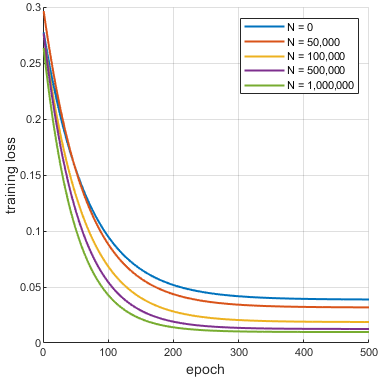
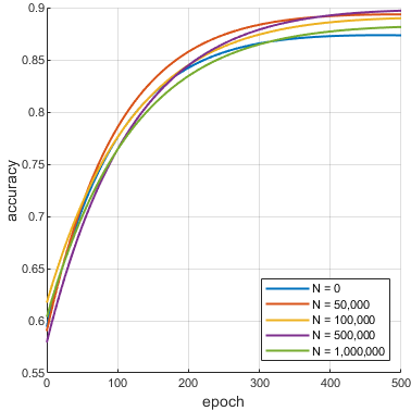
As presented in Section 3.2, we randomly selected 50,000, 100,000, 500,000, and 1,000,000 input pairs among the total of 3,455,881 possible input pairs. Here, we aim to evaluate the contribution of the sampling size ($N$) to the model performance. As shown in Fig. 7, the convergence rate and the final training loss of the model become faster and lower as $N$ increases. However, from $N=100,000$ onwards, the effect gain from increasing $N$ is almost no longer obvious. Fig. 7 illustrates the corresponding classification accuracy of the model for different values of $N$. As can be seen, the sample size $N$ is positively correlated to the accuracy between 50,000 and 100,000, though the difference between them is small. However, the accuracy decreases if the value of $N$ is set too large (i.e., $N=1,000,000$), even though it is still better than the original accuracy. Therefore, taking into account the effect and computational performance, we finally chose $N=100,000$ as the sample size for data augmentation.

Figure 7: Training loss (a) and accuracy (b) curves obtained within 500 epochs using different sample sizes, $N$.

4.4 Analysis of the effects of data augmentation

In this section, we evaluated the impact of our proposed approach as a data augmentation technique for different models selected from the literature. As presented in the previous section, the training sets $\mathcal{T}$, KL-0 and KL-2 of X-ray images were randomly used as input pairs for the proposed KE-CAE model to obtain the corresponding reconstructed and key-exchanged outputs ($\hat{X}$ and $X^{\prime}$). The three sets of data ($X$, $\hat{X}$, and $X^{\prime}$) constitute a larger training set $\mathcal{T^{\prime}}$ for different classification models. For greater convenience, we only selected the learning model from each DenseNet, ResNet, and VGG series that achieved the best performance of the KOA classification in its group (i.e., DenseNet-201, ResNet-18, and VGG-11) [16]. As can be seen in Table 4, four types of input were evaluated for the selected classification models. Regardless of which data ($\hat{X}$ or $X^{\prime}$) were used as additional input, the accuracy of the selected models is always improved. Especially, the combination of $\hat{X}$ and $X^{\prime}$ gave the best performance. More specifically, the performance of the DenseNet-201, ResNet-18, and VGG-11 models increased when the combination of $X$, $\hat{X}$, and $X^{\prime}$ was used as input. Of these, the VGG-11 model has the greatest accuracy gain (+1.98$\%$). However, the Siamese-GAP model achieved the best global accuracy (89.11$\%$). Since the reconstructed output $\hat{X}$ does not have much change to the data structure, the improvement in effect it brings is not significant. On the contrary, compared to the reconstructed output $\hat{X}$, the key-exchanged output $X^{\prime}$ can significantly improve the model accuracy, which demonstrates the efficiency of our proposed approach as a data augmentation technique.

Table 4: Analysis of the applicability on common models

Model	Input	Accuracy ($\%$)	Difference ($\%$)1
DenseNet-201	$X$	84.43	-
	$X$, $\hat{X}$	84.63	0.20 $\uparrow$
	$X$, $X^{\prime}$	85.55	1.12 $\uparrow$
	$X$, $\hat{X}$, $X^{\prime}$	85.64	1.21 $\uparrow$
ResNet-18	$X$	83.59	-
	$X$, $\hat{X}$	83.88	0.29 $\uparrow$
	$X$, $X^{\prime}$	85.11	1.52 $\uparrow$
	$X$, $\hat{X}$, $X^{\prime}$	85.22	1.63 $\uparrow$
VGG-11	$X$	80.97	-
	$X$, $\hat{X}$	81.59	0.62 $\uparrow$
	$X$, $X^{\prime}$	82.83	1.86 $\uparrow$
	$X$, $\hat{X}$, $X^{\prime}$	82.95	1.98 $\uparrow$
Siamese-GAP [16]2	$X$	88.38	-
	$X$, $\hat{X}$	88.51	0.13 $\uparrow$
	$X$, $X^{\prime}$	88.99	0.61 $\uparrow$
	$X$, $\hat{X}$, $X^{\prime}$	89.11	0.73 $\uparrow$

• Obtained accuracy was compared to the accuracy using the original input $X$.

• The parameters of the discriminator were initialized and trained from scratch.

4.5 Discussion

In this paper, we have introduced a new approach for exchanging key features of KL-0 and KL-2 of the knee X-rays to generate new data as an augmentation technique for early KOA classification. Our proposed learning model is a Convolutional Auto-Encoder-based network. For the encoder, dual convolutional layers were used to extract the unrelated and key features. For the decoder, deconvolutional layers were used to reconstruct the feature vectors for the reconstructed $\hat{X}$ and key-exchanged $X^{\prime}$ outputs. To do so, an adequate hybrid loss strategy was proposed, which consists of the combination of the MSE loss, the CE loss and the FDA distance. The three loss functions were optimised using weights $\lambda_{1}$ and $\lambda_{2}$.

Our experimental findings confirmed that the CAE-based model has a high ability for feature extraction and reconstruction, and demonstrated the validity of our proposed approach as a data augmentation technique.

4.5.1 Details of the proposed model

As presented in Section 2.2, convolutional layers were used to extract features instead of classic dense layers. Convolutional layers not only have a smaller number of parameters but can also learn spatial feature information of the input image. Moreover, we used more CNN layers rather than a pooling layer for the down-sampling operation to preserve the spatial information of the X-ray images as much as possible. In addition to this, we also evaluated other variants of Auto-Encoders, such as Variational Auto-Encoders (VAE) [38] and Denoising Auto-Encoders (DAE) [39]. However, no improvement was observed except in increasing the number of parameters.

4.5.2 Strengths and limitations

This study presents several important strengths. From a clinical point of view, it is more clinically meaningful to focus on early knee OA diagnosis (KL-0 vs KL-2) to inform patients to make timely physical interventions and delay the onset and worsening of OA symptoms. To improve a clinically applicable model, we considered multiple steps to enhance its applicability. First, we normalised each original X-ray image to always have a constant ROI (299 $\times$ 299 pixels), which is consistent with the attention areas that radiologists consider when diagnosing KOA [40]. Second, using our approach, new valid data in accordance with the distribution of the original dataset were generated as an effective data augmentation method for the deep-learning-based classification models, which has improved the classification performance of deep-learning-based models. Finally, common data augmentation techniques such as rotation, gamma correction, and jitter were also used to further enhance the stability and robustness of the model. We believe that a more stable model in a Computer-Aided Diagnosis (CAD) system can make deep learning approaches gain more trust and acceptance from medical practitioners in daily clinical practice.

There were also several limitations in our study. All experiments were achieved using the OAI database. Other large databases should be considered to evaluate and strengthen the proposed approach. Moreover, manual tuning of the hyper-parameters in the hybrid loss strategy is machine time-consuming. Therefore, the use of large datasets and automatic adjustment of the hyper-parameters could be of interest for future work.

References

- [1] Richard F Loeser, Steven R Goldring, Carla R Scanzello, and Mary B Goldring. Osteoarthritis: a disease of the joint as an organ. Arthritis and rheumatism, 64(6):1697, 2012.
- [2] Anna Litwic, Mark H. Edwards, Elaine M. Dennison, and Cyrus Cooper. Epidemiology and burden of osteoarthritis. British Medical Bulletin, 105(1):185–199, 01 2013.
- [3] Gurkirpal Singh, Jeffrey D Miller, Fleur H Lee, Dan Pettitt, and Mason W Russell. Prevalence of cardiovascular disease risk factors among us adults with self-reported osteoarthritis: data from the third national health and nutrition examination survey. Population, 7:17, 2002.
- [4] K. Lim and C. Lau. Perception is everything: OA is exciting. International Journal of Rheumatic Diseases, 14(2):111–112, 2011.
- [5] Juan C Mora, Rene Przkora, and Yenisel Cruz-Almeida. Knee osteoarthritis: pathophysiology and current treatment modalities. Journal of pain research, 11:2189, 2018.
- [6] Anita E Wluka, Cate B Lombard, and Flavia M Cicuttini. Tackling obesity in knee osteoarthritis. Nature Reviews Rheumatology, 9(4):225–235, 2013.
- [7] J. H. Kellgren and J. S. Lawrence. Radiological Assessment of Osteo-Arthrosis. Annals of the Rheumatic Diseases, 16(4):494, 1957.
- [8] Lior Shamir, Shari M Ling, William W Scott, Angelo Bos, Nikita Orlov, Tomasz J Macura, D Mark Eckley, Luigi Ferrucci, and Ilya G Goldberg. Knee x-ray image analysis method for automated detection of osteoarthritis. IEEE Transactions on Biomedical Engineering, 56(2):407–415, 2008.
- [9] A. Krizhevsky, I. Sutskever, and G. E Hinton. Imagenet classification with deep convolutional neural networks. Advances in neural information processing systems, 25:1097–1105, 2012.
- [10] Holger R. Roth, Le Lu, Jiamin Liu, Jianhua Yao, Ari Seff, Kevin Cherry, Lauren Kim, and Ronald M. Summers. Improving computer-aided detection using convolutional neural networks and random view aggregation. IEEE Transactions on Medical Imaging, 35(5):1170–1181, 2016.
- [11] Liang Chen, Paul Bentley, Kensaku Mori, Kazunari Misawa, Michitaka Fujiwara, and Daniel Rueckert. Drinet for medical image segmentation. IEEE Transactions on Medical Imaging, 37(11):2453–2462, 2018.
- [12] C.-C. Chen, J.S. DaPonte, and M.D. Fox. Fractal feature analysis and classification in medical imaging. IEEE Transactions on Medical Imaging, 8(2):133–142, 1989.
- [13] J. Antony, K. McGuinness, K. Moran, and N. E O’Connor. Automatic detection of knee joints and quantification of knee osteoarthritis severity using convolutional neural networks. In International conference on machine learning and data mining in pattern recognition, pages 376–390. Springer, 2017.
- [14] J. Long, E. Shelhamer, and T. Darrell. Fully convolutional networks for semantic segmentation. In Proceedings of the IEEE conference on computer vision and pattern recognition, pages 3431–3440, 2015.
- [15] A. Tiulpin, J. Thevenot, E. Rahtu, P. Lehenkari, and S. Saarakkala. Automatic knee osteoarthritis diagnosis from plain radiographs: A deep learning-based approach. Scientific Reports, 2018.
- [16] Zhe Wang, Aladine Chetouani, Didier Hans, Eric Lespessailles, and Rachid Jennane. Siamese-gap network for early detection of knee osteoarthritis. In 2022 IEEE 19th International Symposium on Biomedical Imaging (ISBI), pages 1–4, 2022.
- [17] R. R. Selvaraju, M. Cogswell, A. Das, R. Vedantam, D. Parikh, and D. Batra. Grad-cam: Visual explanations from deep networks via gradient-based localization. In 2017 IEEE International Conference on Computer Vision (ICCV), pages 618–626, 2017.
- [18] Julia Röglin, Katharina Ziegeler, Jana Kube, Franziska König, Kay-Geert Hermann, and Steffen Ortmann. Improving classification results on a small medical dataset using a gan; an outlook for dealing with rare disease datasets. Frontiers in Computer Science, page 102, 2022.
- [19] Connor Shorten and Taghi M Khoshgoftaar. A survey on image data augmentation for deep learning. Journal of big data, 6(1):1–48, 2019.
- [20] Ian Goodfellow, Jean Pouget-Abadie, Mehdi Mirza, Bing Xu, David Warde-Farley, Sherjil Ozair, Aaron Courville, and Yoshua Bengio. Generative adversarial nets. Advances in neural information processing systems, 27, 2014.
- [21] Fabio Henrique Kiyoiti dos Santos Tanaka and Claus Aranha. Data augmentation using gans. arXiv preprint arXiv:1904.09135, 2019.
- [22] Anthony J Myles, Robert N Feudale, Yang Liu, Nathaniel A Woody, and Steven D Brown. An introduction to decision tree modeling. Journal of Chemometrics: A Journal of the Chemometrics Society, 18(6):275–285, 2004.
- [23] Maayan Frid-Adar, Idit Diamant, Eyal Klang, Michal Amitai, Jacob Goldberger, and Hayit Greenspan. Gan-based synthetic medical image augmentation for increased cnn performance in liver lesion classification. Neurocomputing, 321:321–331, 2018.
- [24] Alec Radford, Luke Metz, and Soumith Chintala. Unsupervised representation learning with deep convolutional generative adversarial networks. arXiv preprint arXiv:1511.06434, 2015.
- [25] Farzan Farnia and Asuman Ozdaglar. Do gans always have nash equilibria? In International Conference on Machine Learning, pages 3029–3039. PMLR, 2020.
- [26] Y. Nasser, R. Jennane, A. Chetouani, E. Lespessailles, and M. E. Hassouni. Discriminative regularized auto-encoder for early detection of knee osteoarthritis: Data from the Osteoarthritis Initiative. IEEE Transactions on Medical Imaging, 39(9):2976–2984, 2020.
- [27] Lie Yang, Yong Tian, Yonghao Song, Nachuan Yang, Ke Ma, and Longhan Xie. A novel feature separation model exchange-gan for facial expression recognition. Knowledge-Based Systems, 204:106217, 2020.
- [28] Sebastian Mika, Gunnar Ratsch, Jason Weston, Bernhard Scholkopf, and Klaus-Robert Mullers. Fisher discriminant analysis with kernels. In Neural networks for signal processing IX: Proceedings of the 1999 IEEE signal processing society workshop (cat. no. 98th8468), pages 41–48. Ieee, 1999.
- [29] Ronald A Fisher. The use of multiple measurements in taxonomic problems. Annals of eugenics, 7(2):179–188, 1936.
- [30] G. Lester. The Osteoarthritis Initiative: A NIH Public–Private Partnership. HSS Journal: The Musculoskeletal Journal of Hospital for Special Surgery, 8(1):62–63, 2011.
- [31] Hervé Bourlard and Yves Kamp. Auto-association by multilayer perceptrons and singular value decomposition. Biological cybernetics, 59(4):291–294, 1988.
- [32] Harold Hotelling. Analysis of a complex of statistical variables into principal components. Journal of educational psychology, 24(6):417, 1933.
- [33] P. Chen, L. Gao, X. Shi, K. Allen, and L. Yang. Fully automatic knee osteoarthritis severity grading using deep neural networks with a novel ordinal loss. Computerized Medical Imaging and Graphics, 75:84–92, 2019.
- [34] N. V Chawla, K. W Bowyer, L. O Hall, and W P. Kegelmeyer. Smote: synthetic minority over-sampling technique. Journal of artificial intelligence research, 16:321–357, 2002.
- [35] Kaiming He, Xiangyu Zhang, Shaoqing Ren, and Jian Sun. Delving deep into rectifiers: Surpassing human-level performance on imagenet classification. In Proceedings of the IEEE international conference on computer vision, pages 1026–1034, 2015.
- [36] Adam Paszke, Sam Gross, Francisco Massa, Adam Lerer, James Bradbury, Gregory Chanan, Trevor Killeen, Zeming Lin, Natalia Gimelshein, Luca Antiga, Alban Desmaison, Andreas Köpf, Edward Yang, Zach DeVito, Martin Raison, Alykhan Tejani, Sasank Chilamkurthy, Benoit Steiner, Lu Fang, Junjie Bai, and Soumith Chintala. Pytorch: An imperative style, high-performance deep learning library, 2019.
- [37] Christopher JC Burges. A tutorial on support vector machines for pattern recognition. Data mining and knowledge discovery, 2(2):121–167, 1998.
- [38] Diederik P Kingma and Max Welling. Auto-encoding variational bayes. arXiv preprint arXiv:1312.6114, 2013.
- [39] Pascal Vincent, Hugo Larochelle, Yoshua Bengio, and Pierre-Antoine Manzagol. Extracting and composing robust features with denoising autoencoders. In Proceedings of the 25th international conference on Machine learning, pages 1096–1103, 2008.
- [40] Marta Favero, Roberta Ramonda, Mary B Goldring, Steven R Goldring, and Leonardo Punzi. Early knee osteoarthritis. RMD open, 1(Suppl 1):e000062, 2015.