Diffusion Model-Augmented Behavioral Cloning

Abstract

Imitation learning addresses the challenge of learning by observing an expert’s demonstrations without access to reward signals from environments. Most existing imitation learning methods that do not require interacting with environments either model the expert distribution as the conditional probability $p(a|s)$ (e.g., behavioral cloning, BC) or the joint probability $p(s,a)$. Despite its simplicity, modeling the conditional probability with BC usually struggles with generalization. While modeling the joint probability can improve generalization performance, the inference procedure is often time-consuming, and the model can suffer from manifold overfitting. This work proposes an imitation learning framework that benefits from modeling both the conditional and joint probability of the expert distribution. Our proposed diffusion model-augmented behavioral cloning (DBC) employs a diffusion model trained to model expert behaviors and learns a policy to optimize both the BC loss (conditional) and our proposed diffusion model loss (joint). DBC outperforms baselines in various continuous control tasks in navigation, robot arm manipulation, dexterous manipulation, and locomotion. We design additional experiments to verify the limitations of modeling either the conditional probability or the joint probability of the expert distribution, as well as compare different generative models. Ablation studies justify the effectiveness of our design choices.

1 Introduction

Recently, the success of deep reinforcement learning (DRL) (Mnih et al., 2015; Lillicrap et al., 2016; Arulkumaran et al., 2017) has inspired the research community to develop DRL frameworks to control robots, aiming to automate the process of designing sensing, planning, and control algorithms by letting the robot learn in an end-to-end fashion. Yet, acquiring complex skills through trial and error can still lead to undesired behaviors even with sophisticated reward design (Christiano et al., 2017; Leike et al., 2018; Lee et al., 2019). Moreover, the exploring process could damage expensive robotic platforms or even be dangerous to humans (Garcıa and Fernández, 2015; Levine et al., 2020).

To overcome this issue, imitation learning (i.e., learning from demonstration) (Schaal, 1997; Osa et al., 2018) has received growing attention, whose aim is to learn a policy from expert demonstrations, which are often more accessible than appropriate reward functions for reinforcement learning. Among various imitation learning directions, adversarial imitation learning (Ho and Ermon, 2016; Zolna et al., 2021; Kostrikov et al., 2019) and inverse reinforcement learning (Ng and Russell, 2000; Abbeel and Ng, 2004) have achieved encouraging results in a variety of domains. Yet, these methods require interacting with environments, which can still be expensive or even dangerous.

On the other hand, behavioral cloning (BC) (Pomerleau, 1989; Bain and Sammut, 1995) does not require interacting with environments. BC formulates imitation learning as a supervised learning problem — given an expert demonstration dataset, an agent policy takes states sampled from the dataset as input and learns to replicate the corresponding expert actions. One can view a BC policy as a discriminative model $p(a|s)$ that models the conditional probability of actions $a$ given a state $s$. Due to its simplicity and training stability, BC has been widely adopted for various applications. However, BC struggles at generalizing to states unobserved during training (Nguyen et al., 2023).

To alleviate the generalization issue, we propose to augment BC by modeling the joint probability $p(s,a)$ of expert state-action pairs with a generative model (e.g., diffusion models). This is motivated by Bishop and Nasrabadi (2006) and  Fisch et al. (2013), who illustrate that modeling joint probability allows for better generalizing to data points unobserved during training. However, with a learned joint probability model $p(s,a)$, retrieving a desired action $a$ requires actions sampling and optimization (i.e., $\underset{a\in\mathcal{A}}{\arg\max}\ p(s,a)$), which can be extremely inefficient with a large action space. Moreover, modeling joint probabilities can suffer from manifold overfitting (Wu et al., 2021; Loaiza-Ganem et al., 2022) when observed high-dimensional data lies on a low-dimensional manifold (e.g., state-action pairs collected from a script expert policies).

This work proposes an imitation learning framework that combines both the efficiency and stability of modeling the conditional probability and the generalization ability of modeling the joint probability. Specifically, we propose to model the expert state-action pairs using a state-of-the-art generative model, a diffusion model, which learns to estimate how likely a state-action pair is sampled from the expert dataset. Then, we train a policy to optimize both the BC objective and the estimate produced by the learned diffusion model. Therefore, our proposed framework not only can efficiently predict actions given states via capturing the conditional probability $p(a|s)$ but also enjoys the generalization ability induced by modeling the joint probability $p(s,a)$ and utilizing it to guide policy learning.

We evaluate our proposed framework and baselines in various continuous control domains, including navigation, robot arm manipulation, and locomotion. The experimental results show that the proposed framework outperforms all the baselines or achieves competitive performance on all tasks. Extensive ablation studies compare our proposed method to its variants, justifying our design choices, such as different generative models, and investigating the effect of hyperparameters.

2 Related Work

Imitation learning addresses the challenge of learning by observing expert demonstrations without access to reward signals from environments. It has various applications such as robotics (Schaal, 1997; Zhao et al., 2023), autonomous driving (Ly and Akhloufi, 2020), and game AI (Harmer et al., 2018).

Behavioral Cloning (BC). BC (Pomerleau, 1989; Torabi et al., 2018) formulates imitating an expert as a supervised learning problem. Due to its simplicity and effectiveness, it has been widely adopted in various domains. Yet, it often struggles at generalizing to states unobserved from the expert demonstrations (Ross et al., 2011; Florence et al., 2022). Some approaches prevent the state from drifting off the expert demonstrations by mitigating compounding error (Ross et al., 2011; Zhao et al., 2023). However, the problem of generalization still exists even when the compounding errors are alleviated. In this work, we improve the generalization ability of policies by augmenting BC with a diffusion model that learns to capture the joint probability of expert state-action pairs.

Adversarial Imitation Learning (AIL). AIL methods aim to match the state-action distributions of an agent and an expert via adversarial training. Generative adversarial imitation learning (GAIL) (Ho and Ermon, 2016) and its extensions (Torabi et al., 2019; Kostrikov et al., 2019; Zolna et al., 2021; Jena et al., 2021) resemble the idea of generative adversarial networks (Goodfellow et al., 2014), which trains a generator policy to imitate expert behaviors and a discriminator to distinguish between the expert and the learner’s state-action pair distributions. While modeling state-action distributions often leads to satisfactory performance, adversarial learning can be unstable and inefficient (Chen et al., 2020). Moreover, even though scholars like  Jena et al. (2021) propose to improve the efficiency of GAIL with the BC loss, they still require online interaction with environments, which can be costly or even dangerous. In contrast, our work does not require interacting with environments.

Inverse Reinforcement Learning (IRL). IRL methods (Ng and Russell, 2000; Abbeel and Ng, 2004; Fu et al., 2018; Lee et al., 2021) are designed to infer the reward function that underlies the expert demonstrations and then learn a policy using the inferred reward function. This allows for learning tasks whose reward functions are difficult to specify manually. However, due to its double-loop learning procedure, IRL methods are typically computationally expensive and time-consuming. Additionally, obtaining accurate estimates of the expert’s reward function can be difficult, especially when the expert’s behavior is non-deterministic or when the expert’s demonstrations are sub-optimal.

Diffusion Policies. Recently, Pearce et al. (2023); Chi et al. (2023); Reuss et al. (2023) propose to represent and learn an imitation learning policy using a conditional diffusion model, which produces a predicted action conditioning on a state and a sampled noise vector. These methods achieve encouraging results in modeling stochastic and multimodal behaviors from human experts or play data. In contrast, instead of representing a policy using a diffusion model, our work employs a diffusion model trained on expert demonstrations to guide a policy as a learning objective.

3 Preliminaries

3.1 Imitation Learning

In contrast to reinforcement learning, whose goal is to learn a policy $\pi$ based on rewards received while interacting with the environment, imitation learning methods aim to learn the policy from an expert demonstration dataset containing $M$ trajectories, $D=\{\tau_{1},...,\tau_{M}\}$, where $\tau_{i}$ represents a sequence of $n_{i}$ state-action pairs $\{s^{i}_{1},a^{i}_{1},...,s^{i}_{n_{i}},a^{i}_{n_{i}}\}$.

3.1.1 Modeling Conditional Probability $p(a|s)$

To learn a policy $\pi$, behavioral cloning (BC) directly estimates the expert policy $\pi^{E}$ with maximum likelihood estimation (MLE). Given a state-action pair $(s,a)$ sampled from the dataset $D$, BC optimizes $\mathop{max}\limits_{\theta}\sum\limits_{(s,a)\in D}\log(\pi_{\theta}(a|s))$, where $\theta$ denotes the parameters of the policy $\pi$. One can view a BC policy as a discriminative model $p(a|s)$, capturing the conditional probability of an action $a$ given a state $s$.

Despite its success in various applications, BC tends to overfit and struggle at generalizing to states unseen during training (Ross et al., 2011; Codevilla et al., 2019; Wang et al., 2022).

3.1.2 Modeling Joint Probability $p(s,a)$

On the other hand, modeling the joint probability can yield improved generalization performance, as illustrated in Bishop and Nasrabadi (2006); Fisch et al. (2013). For instance, Florence et al. (2022); Ganapathi et al. (2022) propose to model the joint probability $p(s,a)$ of expert state-action pairs using an energy-based model. Then, during inference, a gradient-free optimizer is used to retrieve a desired action $a$ by sampling and optimizing actions (i.e., $\arg\max_{a\in\mathcal{A}}\ p(s,a)$). Despite its success in various domains, it can be extremely inefficient to retrieve actions with a large action space.

Moreover, explicit generative models such as energy-based models (Du and Mordatch, 2019; Song and Kingma, 2021), variational autoencoder (Kingma and Welling, 2014), and flow-based models (Rezende and Mohamed, 2015; Dinh et al., 2017) are known to struggle with modeling observed high-dimensional data that lies on a low-dimensional manifold (i.e., manifold overfitting) (Wu et al., 2021; Loaiza-Ganem et al., 2022). As a result, these methods often perform poorly when learning from demonstrations produced by script policies or PID controllers, as discussed in Section 5.4.

We aim to develop an imitation learning framework that enjoys the advantages of modeling the conditional probability $p(a|s)$ and the joint probability $p(s,a)$. Specifically, we propose to model the joint probability of expert state-action pairs using an explicit generative model $\phi$, which learns to produce an estimate indicating how likely a state-action pair is sampled from the expert dataset. Then, we train a policy to model the conditional probability $p(a|s)$ by optimizing the BC objective and the estimate produced by the learned generative model $\phi$. Hence, our method can efficiently predict actions given states, generalize better to unseen states, and suffer less from manifold overfitting.

Figure 1: Denoising Diffusion Probabilistic Model (DDPM). Latent variables $x_{1},...,x_{N}$ are produced from the data point $x_{0}$ via the forward diffusion process, i.e., gradually adding noises to the latent variables. The diffusion model $\phi$ learns to reverse the diffusion process by denoising the noisy data to reconstruct the original data point $x_{0}$.

3.2 Diffusion Models

As described in the previous sections, this work aims to combine the advantages of modeling the conditional probability $p(a|s)$ and the joint probability $p(s,a)$. Hence, we leverage diffusion models to model the joint probability of expert state-action pairs. The diffusion model is a recently developed class of generative models and has achieved state-of-the-art performance on various tasks (Sohl-Dickstein et al., 2015; Nichol and Dhariwal, 2021; Dhariwal and Nichol, 2021; Ko et al., 2023).

In this work, we utilize Denoising Diffusion Probabilistic Models (DDPMs) (J Ho, 2020) to model expert state-action pairs. Specifically, DDPM models gradually add noise to data samples (i.e., concatenated state-action pairs) until they become isotropic Gaussian (forward diffusion process), and then learn to denoise each step and restore the original data samples (reverse diffusion process), as illustrated in Figure 1. In other words, DDPM learns to recognize a data distribution by learning to denoise noisy sampled data. More discussion on diffusion models can be found in the  Section J.

4 Approach

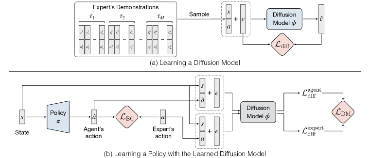
Our goal is to design an imitation learning framework that enjoys both the advantages of modeling the conditional probability and the joint probability of expert behaviors. To this end, we first adopt behavioral cloning (BC) for modeling the conditional probability from expert state-action pairs, as described in Section 4.1. To capture the joint probability of expert state-action pairs, we employ a diffusion model which learns to produce an estimate indicating how likely a state-action pair is sampled from the expert state-action pair distribution, as presented in Section 4.2.1. Then, we propose to guide the policy learning by optimizing this estimate provided by a learned diffusion model, encouraging the policy to produce actions similar to expert actions, as discussed in Section 4.2.2. Finally, in Section 4.3, we introduce the framework that combines the BC loss and our proposed diffusion model loss, allowing for learning a policy that benefits from modeling both the conditional probability and the joint probability of expert behaviors. An overview of our proposed framework is illustrated in Figure 2, and the algorithm is detailed in Section A.

4.1 Behavioral Cloning Loss

The behavioral cloning (BC) model aims to imitate expert behaviors with supervision learning. BC learns to capture the conditional probability $p(a|s)$ of expert state-action pairs. A BC policy $\pi(a|s)$ learns by optimizing

$$\mathcal{L}_{\text{BC}}=\mathbb{E}_{(s,a)\sim D,\hat{a}\sim\pi(s)}[d(a,\hat{a})],$$ (1)

where $d(\cdot,\cdot)$ denotes a distance measure between a pair of actions. For example, we can adapt the mean-square error (MSE) loss ${||a-\hat{a}||}^{2}$ for most continuous control tasks.

4.2 Learning a Diffusion Model and Guiding Policy Learning

Instead of directly learning the conditional probability $p(a|s)$, this section discusses how to model the joint probability $p(s,a)$ of expert behaviors with a diffusion model in Section 4.2.1 and presents how to leverage the learned diffusion model to guide policy learning in Section 4.2.2.

Figure 2: Diffusion Model-Augmented Behavioral Cloning. Our proposed method DBC augments behavioral cloning (BC) by employing a diffusion model. (a) Learning a Diffusion Model: the diffusion model $\phi$ learns to model the distribution of concatenated state-action pairs sampled from the demonstration dataset $D$. It learns to reverse the diffusion process (i.e., denoise) by optimizing $\mathcal{L}_{\text{diff}}$ in Eq. 2. (b) Learning a Policy with the Learned Diffusion Model: we propose a diffusion model objective $\mathcal{L}_{\text{DM}}$ for policy learning and jointly optimize it with the BC objective $\mathcal{L}_{\text{BC}}$. Specifically, $\mathcal{L}_{\text{DM}}$ is computed based on processing a sampled state-action pair $(s,a)$ and a state-action pair $(s,\hat{a})$ with the action $\hat{a}$ predicted by the policy $\pi$ with $\mathcal{L}_{\text{diff}}$.

4.2.1 Learning a Diffusion Model

We propose to model the joint probability of expert state-action pairs with a diffusion model $\phi$. Specifically, we create a joint distribution by simply concatenating a state vector $s$ and an action vector $a$ from a state-action pair $(s,a)$. To model such distribution by learning a denoising diffusion probabilistic model (DDPM) (J Ho, 2020), we inject noise $\epsilon(n)$ into sampled state-action pairs, where $n$ indicates the number of steps of the Markov procedure, which can be viewed as a variable of the level of noise, and the total number of steps is notated as $N$. Then, we train the diffusion model $\phi$ to predict the injected noises by optimizing

$$\mathcal{L}_{\text{diff}}(s,a,\phi)=\mathbb{E}_{n\sim N,(s,a)\sim D}\left[{||\hat{\epsilon}(s,a,n)-\epsilon(n)||}^{2}\right]$$ (2)

$$=\mathbb{E}_{n\sim N,(s,a)\sim D}\left[{||\phi(s,a,\epsilon(n))-\epsilon(n)||}^{2}\right],$$

where $\hat{\epsilon}$ is the noise predicted by the diffusion model $\phi$. Once optimized, the diffusion model can recognize the expert distribution by perfectly predicting the noise injected into state-action pairs sampled from the expert distribution. On the other hand, predicting the noise injected into state-action pairs sampled from any other distribution should yield a higher loss value. Therefore, we propose to view $\mathcal{L}_{\text{diff}}(s,a,\phi)$ as an estimate of how well the state-action pair $(s,a)$ fits the state-action distribution that $\phi$ learns from.

4.2.2 Learning a Policy with Diffusion Model Loss

A diffusion model $\phi$ trained on an expert dataset can produce an estimate $\mathcal{L}_{\text{diff}}(s,a,\phi)$ indicating how well a state-action pair $(s,a)$ fits the expert distribution. We propose to leverage this signal to guide a policy $\pi$ predicting actions $\hat{a}$ to imitate the expert. Specifically, the policy $\pi$ learns by optimizing

$$\mathcal{L}_{\text{diff}}^{\text{agent}}=\mathcal{L}_{\text{diff}}(s,\hat{a},\phi)=\mathbb{E}_{s\sim D,\hat{a}\sim\pi(s)}\left[{||\hat{\epsilon}(s,\hat{a},n)-\epsilon||}^{2}\right].$$ (3)

Intuitively, the policy $\pi$ learns to predict actions $\hat{a}$ that are indistinguishable from the expert actions $a$ for the diffusion model conditioning on the same set of states.

We hypothesize that learning a policy to optimize Eq. 3 can be unstable, especially for state-action pairs that are not well-modeled by the diffusion model, which yield a high value of $\mathcal{L}_{\text{diff}}$ even with expert state-action pairs. Therefore, we propose to normalize the agent diffusion loss $\mathcal{L}_{\text{diff}}^{\text{agent}}$ with an expert diffusion loss $\mathcal{L}_{\text{diff}}^{\text{expert}}$, which can be computed with expert state-action pairs $(s,a)$ as follows:

$$\mathcal{L}_{\text{diff}}^{\text{expert}}=\mathcal{L}_{\text{diff}}(s,a,\phi)=\mathbb{E}_{(s,a)\sim D}\left[{||\hat{\epsilon}(s,a,n)-\epsilon||}^{2}\right].$$ (4)

We propose to optimize the diffusion model loss $\mathcal{L}_{\text{DM}}$ based on calculating the difference between the above agent and expert diffusion losses:

$$\mathcal{L}_{\text{DM}}=\mathbb{E}_{(s,a)\sim D,\hat{a}\sim\pi(s)}\left[max\left(\mathcal{L}_{\text{diff}}^{\text{agent}}-\mathcal{L}_{\text{diff}}^{\text{expert}},0\right)\right].$$ (5)

4.3 Combining the Two Objectives

Our goal is to learn a policy that benefits from both modeling the conditional probability and the joint probability of expert behaviors. To this end, we propose to augment a BC policy, which optimizes the BC loss $L_{\text{BC}}$ in Eq. 1, by combining $L_{\text{BC}}$ with the proposed diffusion model loss $L_{\text{DM}}$ in Eq. 5. By optimizing them together, we encourage the policy to predict actions that fit the expert joint probability captured by diffusion models. To learn from both the BC loss and the diffusion model loss, we train the policy to optimize

$$\mathcal{L}_{\text{total}}=\mathcal{L}_{\text{BC}}+\lambda\mathcal{L}_{\text{DM}},$$ (6)

where $\lambda$ is a coefficient that determines the importance of the diffusion model loss relative to the BC loss. Our experimental results empirically show that optimizing a combination of the BC loss $\mathcal{L}_{\text{BC}}$ and the diffusion model loss $\mathcal{L}_{\text{DM}}$ leads to the best performance compared to solely optimizing each of them, highlighting the effectiveness of the proposed combined loss $\mathcal{L}_{\text{total}}$. Further discussions on combing these two losses can be found in Section B.

(a) Maze

(b) FetchPick

(c) HandRotate

(d) Cheetah

(e) Walker

(f) AntReach

Figure 3: Environments & Tasks. (a) Maze: A point-mass agent (green) in a 2D maze learns to navigate from its start location to a goal location (red). (b) FetchPick: The robot arm manipulation tasks employ a 7-DoF Fetch robotics arm to pick up an object (yellow cube) from the table and move it to a target location (red). (c) HandRotate: This dexterous manipulation task requires a Shadow Dexterous Hand to in-hand rotate a block to a target orientation. (d)-(e) Cheetah and Walker: These locomotion tasks require learning agents to walk as fast as possible while maintaining their balance. (f) AntReach: This task combines locomotion and navigation, instructing an ant robot with four legs to reach a goal location while maintaining balance.

5 Experiments

We design experiments in various continuous control domains, including navigation, robot arm manipulation, dexterous manipulation, and locomotion, to compare our proposed framework (DBC) to its variants and baselines.

5.1 Experimental Setup

This section describes the environments, tasks, and expert demonstrations used for learning and evaluation. More details can be found in Section E.

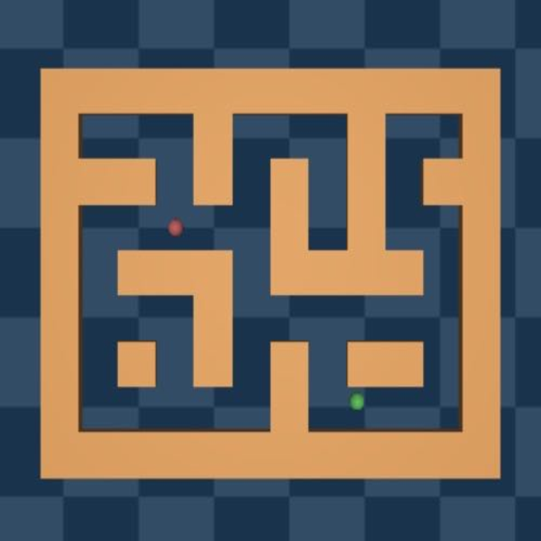
Navigation. To evaluate our method on a navigation task, we choose Maze, a maze environment proposed in (Fu et al., 2020) (maze2d-medium-v2), as illustrated in Figure 3(a). This task features a point-mass agent in a 2D maze learning to navigate from its start location to a goal location by iteratively predicting its $x$ and $y$ acceleration. The agent’s beginning and final locations are chosen randomly. We collect 100 demonstrations with 18,525 transitions using a controller.

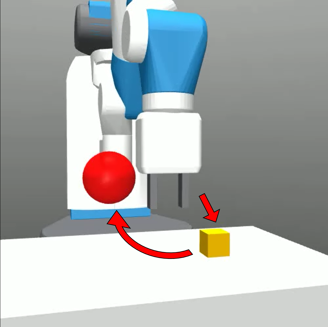
Robot Arm Manipulation. We evaluate our method in FetchPick, a robot arm manipulation domain with a 7-DoF Fetch task, as illustrated in Figure 3(b). FetchPick requires picking up an object from the table and lifting it to a target location. We use the demonstrations, consisting of 10k transitions (303 trajectories), provided by Lee et al. (2021) for these tasks.

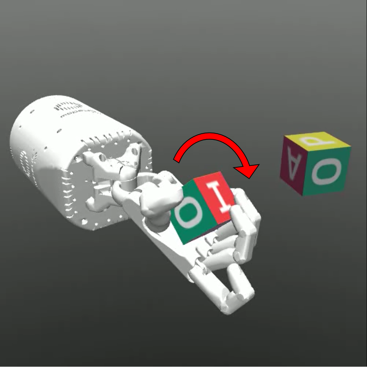
Dexterous Manipulation. In HandRotate, we further evaluate our method on a challenging environment proposed in Plappert et al. (2018), where a 24-DoF Shadow Dexterous Hand learns to in-hand rotate a block to a target orientation, as illustrated in Figure 3(c). This environment has a state space (68D) and action space (20D), which is high dimensional compared to the commonly-used environments in IL. We collected 10k transitions (515 trajectories) from a SAC (Haarnoja et al., 2018) expert policy trained for 10M environment steps.

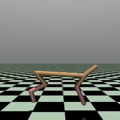
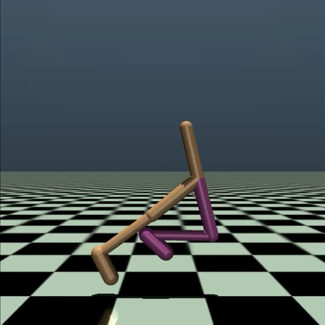
Locomotion. For locomotion, we leverage the Cheetah and Walker (Brockman et al., 2016) environments. Both Cheetah and Walker require a bipedal agent (with different structures) to travel as fast as possible while maintaining its balance, as illustrated in Figure 3(d) and Figure 3(e), respectively. We use the demonstrations provided by Kostrikov (2018), which contains 5 trajectories with 5k state-action pairs for both the Cheetah and Walker environments.

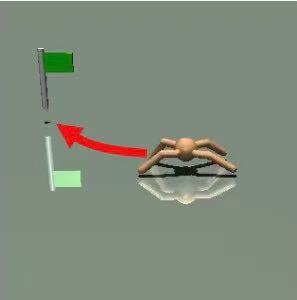
Locomotion + Navigation. We further explore our method on the challenging AntReach environment. In the environment, the quadruped ant aims to reach a randomly generated target located along the boundary of a semicircle centered around the ant, as illustrated in Figure 3(f). AntReach environment combines the properties of locomotion and goal-directed navigation tasks, which require robot controlling and path planning to reach the goal. We use the demonstrations provided by Lee et al. (2021), which contains 500 trajectories with 25k state-action pairs in AntReach.

5.2 Baselines

This work focuses on imitation learning problem without environment interactions. Therefore, approaches that require environmental interactions, such as GAIL-based methods, are not applicable. Instead, we extensively compared our proposed method to state-of-the-art imitation learning methods that do not require interaction with the environment, including Implicit BC (Florence et al., 2022) and Diffusion Policy (Chi et al., 2023; Reuss et al., 2023).

• BC learns to imitate an expert by modeling the conditional probability $p(a|s)$ of the expert behaviors via optimizing the BC loss $\mathcal{L}_{\text{BC}}$ in Eq. 1.

• Implicit BC (IBC) (Florence et al., 2022) models expert state-action pairs with an energy-based model. For inference, we implement the derivative-free optimization algorithm proposed in IBC, which samples actions iteratively and select the desired action according to the predicted energies.

• Diffusion policy refers to the methods that learn a conditional diffusion model as a policy (Chi et al., 2023; Reuss et al., 2023). Specifically, we implement this baseline based on Pearce et al. (2023). We include this baseline to analyze the effectiveness of using diffusion models as a policy or as a learning objective (ours).

Table 1: Experimental Result. We report the mean and the standard deviation of success rate (Maze, FetchPick, HandRotate, AntReach) and return (Cheetah, Walker), evaluated over three random seeds. Our proposed method (DBC) outperforms or performs competitively against the best baseline over all environments.

Method	Maze	FetchPick	HandRotate	Cheetah	Walker	AntReach
BC	92.1% $\pm$ 3.6%	91.6% $\pm$ 5.8%	57.5% $\pm$ 4.7%	4873.3 $\pm$ 69.7	6954.4 $\pm$ 73.5	73.1% $\pm$ 4.0%
Implicit BC	78.3% $\pm$ 6.0%	69.4% $\pm$ 7.3%	13.8% $\pm$ 3.7%	1563.6 $\pm$ 486.8	839.8 $\pm$ 104.2	39.9% $\pm$ 7.3%
Diffusion Policy	95.5% $\pm$ 1.9%	93.9% $\pm$ 3.4%	61.7% $\pm$ 4.1%	4650.3 $\pm$ 59.9	6479.1 $\pm$ 238.6	66.5% $\pm$ 4.5%
DBC (Ours)	95.4% $\pm$ 1.7%	97.5% $\pm$ 1.9%	60.1% $\pm$ 4.4%	4909.5 $\pm$ 73.0	7034.6 $\pm$ 33.7	76.5% $\pm$ 3.7%

5.3 Experimental Results

We report the experimental results in terms of success rate (Maze, FetchPick, HandRotate, and AntReach), and return (Cheetah and Walker) in Table 1. The details of model architecture can be found in Section F. Training and evaluation details can be found in Section G. Additional analysis and experimental results can be found in Section 5.5 and Section I.

Overall Task Performance. In navigation (Maze) and manipulation (FetchPick and HandRotate) tasks, our DBC performs competitively, i.e., within a standard deviation, against the Diffusion Policy and outperforms the other baselines. We hypothesize that these tasks require the agent to learn from demonstrations with various behaviors. Diffusion policy has shown promising performance for capturing multi-modality distribution, while our DBC can also generalize well with the guidance of the diffusion models, so both methods achieve satisfactory results.

In tasks that locomotion is involved, i.e., Cheetah, Walker, and AntReach, our DBC outperforms Diffusion Policy and performs competitively against the simple BC baseline. We hypothesize that this is because locomotion tasks with sufficient expert demonstrations and little randomness do not require generalization during inference. The agent can simply follow the closed-loop progress of the expert demonstrations, resulting in both BC and DBC performing similarly to the expert demonstrations. On the other hand, the Diffusion Policy is designed for modeling multimodal behaviors and therefore performs inferior results on single-mode locomotion tasks.

In summary, our proposed DBC is able to perform superior results on all tasks, which verifies the effectiveness of combining conditional and joint distribution modeling.

(a)

(b)

(c)

Figure 4: Comparing Modeling Conditional Probability and Joint Probability. (a) Generalization. We collect expert trajectories from a PPO policy learning to navigate to goals sampled from the green regions. Then, we learn a policy $\pi_{BC}$ to optimize $\mathcal{L}_{\text{BC}}$, and another policy $\pi_{DM}$ to optimize $\mathcal{L}_{\text{DM}}$ with a diffusion model trained on the expert distribution. We evaluate the two policies by sampling goals from the red regions, which requires the ability to generalize. $\pi_{BC}$ (orange) struggles at generalizing to unseen goals, whereas $\pi_{DM}$ (blue) can generalize (i.e., extrapolate) to some extent. (b)-(c) Manifold overfitting. We collect the green spiral trajectories from a script policy, whose actions are visualized as red crosses. We then train and evaluate $\pi_{BC}$ and $\pi_{DM}$. The trajectories of $\pi_{BC}$ (orange) can closely follow the expert trajectories (green), while the trajectories of $\pi_{DM}$ (blue) deviates from expert’s. This is because the diffusion model struggles at modeling such expert action distribution with a lower intrinsic dimension, which can be observed from incorrectly predicted actions (blue dots) produced by the diffusion model.

Inference Efficiency. To evaluate the inference efficiency, we measure and report the number of evaluation episodes per second ($\uparrow$) for Implicit BC (9.92), Diffusion Policy (1.38), and DBC (30.79) on an NVIDIA RTX 3080 Ti GPU in Maze. As a results of modeling the conditional probability $p(a|s)$, DBC and BC can directly map states to actions during inference. In contrast, Implicit BC samples and optimizes actions, while Diffusion Policy iteratively denoises sampled noises, which are both time-consuming. This verifies the efficiency of modeling the conditional probability.

Action Space Dimension. The Implicit BC baseline requires time-consuming action sampling and optimization during inference, and such a procedure may not scale well to high-dimensional action spaces. Our Implicit BC baseline with a derivative-free optimizer struggles in HandRotate and Walker environments, whose action dimensions are 20 and 6 respectively. This is consistent with Florence et al. (2022), which reports that the optimizer failed to solve tasks with an action dimension larger than 5. In contrast, our proposed DBC can handle high-dimensional action spaces.

5.4 Comparing Modeling Conditional Probability and Joint Probability

This section aims to empirically identify the limitations of modeling either the conditional or the joint probability in an open maze environment implemented with Fu et al. (2020).

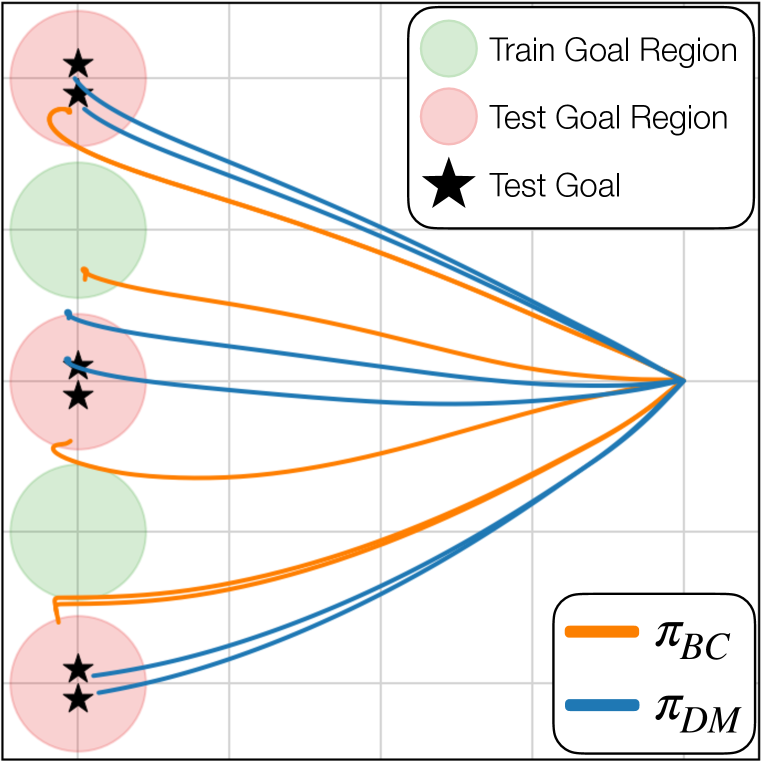
Generalization. We aim to investigate if learning from the BC loss alone struggles at generalization (conditional) and examine if guiding the policy using the diffusion model loss yields improved generalization ability (joint). We collect trajectories of a PPO policy learning to navigate from $(5,3)$ to goals sampled around $(1,2)$ and $(1,4)$ (green) on a 5 $\times$ 5 map, as shown in Figure 4(a). Given these expert trajectories, we learn a policy $\pi_{BC}$ to optimize Eq. 1 and another policy $\pi_{DM}$ to optimize Eq. 5. Then, we evaluate the two policies by sampling goals around $(1,1)$, $(1,3)$, and $(1,5)$ (red), which are unseen during training and require the ability to generalize. Visualized trajectories of the two policies in Figure 4(a) show that $\pi_{BC}$ (orange) fails to generalize to unseen goals, whereas $\pi_{DM}$ (blue) can generalize (i.e., extrapolate) to some extent. This verifies our motivation to augment BC with the diffusion model loss.

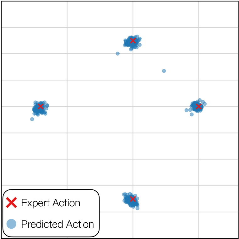
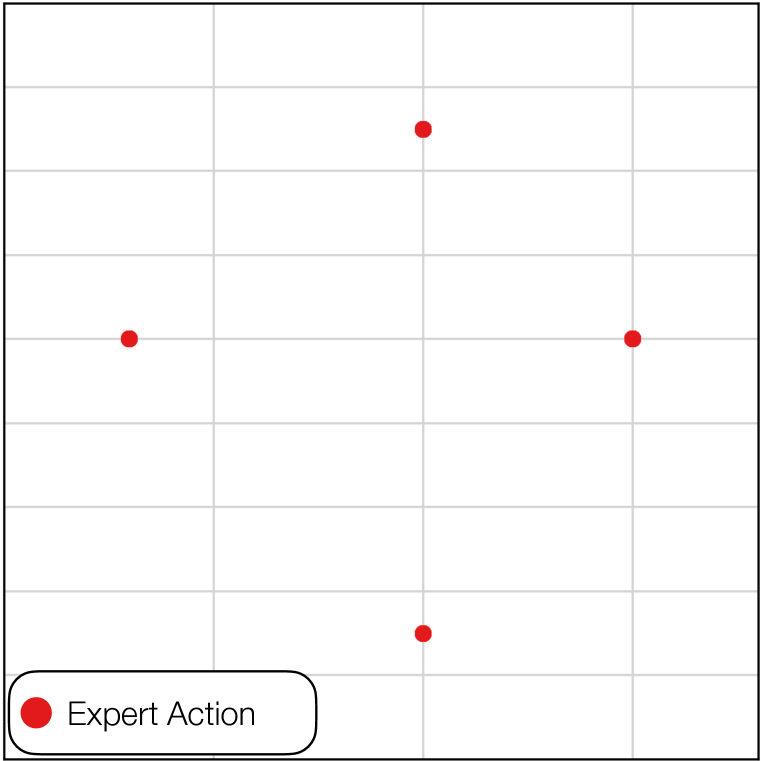
Manifold overfitting. We aim to examine if modeling the joint probability is difficult when observed high-dimensional data lies on a low-dimensional manifold (i.e., manifold overfitting). We collect trajectories from a script policy that executes actions $(0.5,0)$, $(0,0.5)$, $(-0.7,0)$, and $(0,-0.7)$ (red crosses in Figure 4(b)), each for 40 consecutive time steps, resulting the green spiral trajectories visualized in Figure 4(c).

Given these expert demonstrations, we learn a policy $\pi_{BC}$ to optimize Eq. 1, and another policy $\pi_{DM}$ to optimize Eq. 5 with a diffusion model trained on the expert distribution. Figure 4(b) shows that the diffusion model struggles at modeling such expert action distribution with a lower intrinsic dimension. As a result, Figure 4(c) show that the trajectories of $\pi_{DM}$ (blue) deviates from the expert trajectories (green) as the diffusion model cannot provide effective loss. On the other hand, the trajectories of $\pi_{BC}$ (orange) are able to closely follow the expert’s and result in a superior success rate. This verifies our motivation to complement modeling the joint probability with modeling the conditional probability (i.e., BC).

5.5 Generalization Experiments in FetchPick

Table 2: FetchPick Generalization Experimental Result. We report the performance of our proposed framework DBC and the baselines regarding the mean and the standard deviation of the success rate with different levels of noise injected into the initial state and goal locations in FetchPick, evaluated over three random seeds.

Method	Noise Level
	1	1.25	1.5	1.75	2
BC	92.4% $\pm$ 8.5%	91.6% $\pm$ 5.8%	85.5% $\pm$ 6.3%	77.6% $\pm$ 7.1%	67.4% $\pm$ 8.2%
Implicit BC	83.1% $\pm$ 3.1%	69.4% $\pm$ 7.3%	51.6% $\pm$ 4.2%	36.5% $\pm$ 4.7%	23.6% $\pm$ 3.0%
Diffusion Policy	90.0% $\pm$ 3.5%	83.9% $\pm$ 3.4%	72.3% $\pm$ 6.8%	64.1% $\pm$ 7.1%	58.2% $\pm$ 8.2%
DBC (Ours)	99.5% $\pm$ 0.5%	97.5% $\pm$ 1.9%	91.5% $\pm$ 3.3%	83.3% $\pm$ 4.8%	73.5% $\pm$ 6.8%

This section further investigates the generalization capabilities of the policies learned by our proposed framework and the baselines. To this end, we evaluate the policies by injecting different noise levels to both the initial state and goal location in FetchPick. Specifically, we parameterize the noise by scaling the 2D sampling regions for the block and goal locations in both environments. We expect all the methods to perform worse with higher noise levels, while the performance drop of the methods with better generalization ability is less significant. In this experiment, we set the coefficient $\lambda$ of DBC to $0.1$ in FetchPick. The results are presented in Table 2 for FetchPick.

Overall Performance. Our proposed framework DBC consistently outperforms all the baselines with different noise levels, indicating the superiority of DBC when different levels of generalization are required.

Performance Drop with Increased Noise Level. In FetchPick, DBC experiences a performance drop of $26.1\%$ when the noise level increase from $1$ to $2$. However, BC and Implicit BC demonstrate a performance drop of $27.0\%$ and $71.6\%$, respectively. Notably, Diffusion Policy initially performs poorly at a noise level of $1$ but demonstrates its robustness with a performance drop of only $35.3\%$ when the noise level increases to $2$. This demonstrates that our proposed framework not only generalizes better but also exhibits greater robustness to noise compared to the baselines.

5.6 Comparing Different Generative Models

Our proposed framework employs a diffusion model (DM) to model the joint probability of expert state-action pairs and utilizes it to guide policy learning. To justify our choice, we explore using other popular generative models to replace the diffusion model in Maze. We consider energy-based models (EBMs) (Du and Mordatch, 2019; Song and Kingma, 2021), variational autoencoder (VAEs) (Kingma and Welling, 2014), and generative adversarial networks (GANs) (Goodfellow et al., 2014). Each generative model learns to model expert state-action pairs. To guide policy learning, given a predicted state-action pair $(s,\hat{a})$ we use the estimated energy of an EBM, the reconstruction error of a VAE, and the discriminator output of a GAN to optimize a policy with or without the BC loss.

Table 3 compares using different generative models to model the expert distribution and guide policy learning. All the generative model-guide policies can be improved by adding the BC loss, justifying our motivation to complement modeling the joint probability with modeling the conditional probability. With or without the BC loss, the diffusion model-guided policy achieves the best performance compared to other generative models. Specifically, DM outperforms the second-best baseline GAN by 24.8% improvement without BC and by 2.4% with BC, which verifies our choice of the generative model.

Training details of learning generative models and utilizing them to guide policy learning can be found in Section G.4. We report the results on Maze in the main paper because, in the absence of the BC loss, the Maze environment performs reasonably well, unlike FetchPick, which performs poorly. The results on FetchPick can be found in Section H.1

5.7 Ablation Study

Table 3: Generative Models. We compare using different generative models to model the expert distribution and guide policy learning in Maze.

Method	without BC	with BC
BC	N/A	92.1% $\pm$ 3.6%
EBM	20.3% $\pm$ 11.8%	92.5% $\pm$ 3.0%
VAE	53.1% $\pm$ 8.7%	92.7% $\pm$ 2.7%
GAN	54.8% $\pm$ 4.4%	93.0% $\pm$ 3.5%
DM	79.6% $\pm$ 9.6%	95.4% $\pm$ 1.7%

Figure 5: Effect of the Diffusion Model Loss Coefficient $\lambda$. We experiment with different values of $\lambda$ in FetchPick, each evaluated over three random seeds.

5.7.1 Effect of the Diffusion Model Loss Coefficient $\lambda$

We examine the impact of varying the coefficient of the diffusion model loss $\lambda$ in Eq. 6 in FetchPick. The result presented in Figure 3 shows that $\lambda=0.5$ yields the best performance of $97.5\%$. A higher or lower $\lambda$ leads to worse performance. For instance, when $\lambda$ is 0 (only BC), the success rate is $91.7\%$, and the performance drops to $51.46\%$ when $\lambda$ is 10. This result demonstrates that modeling the conditional probability ($\mathcal{L}_{\text{BC}}$) and the joint probability ($\mathcal{L}_{\text{DM}}$) can complement each other.

5.7.2 Effect of the Normalization Term

We aim to investigate whether normalizing the diffusion model loss $\mathcal{L}_{\text{DM}}$ with the expert diffusion model loss $\mathcal{L}_{\text{diff}}^{\text{expert}}$ yields improved performance. We train a variant of DBC where only $\mathcal{L}_{\text{diff}}^{\text{agent}}$ in Eq. 3 instead of $\mathcal{L}_{\text{DM}}$ in Eq. 5 is used to augment BC. For instance, the unnormalized variant performs worse than DBC in the Maze environment, where the average success rate is $94\%$ and $95\%$, respectively. This justifies the effectiveness of the proposed normalization term $\mathcal{L}_{\text{diff}}^{\text{expert}}$ in $\mathcal{L}_{\text{DM}}$. We find consistent results in all of the environments except AntReach, and comprehensive results can be found in Table 8 of  Section H.2

6 Conclusion

We propose an imitation learning framework that benefits from modeling both the conditional probability $p(a|s)$ and the joint probability $p(s,a)$ of the expert distribution. Our proposed diffusion model-augmented behavioral cloning (DBC) employs a diffusion model trained to model expert behaviors and learns a policy to optimize both the BC loss and our proposed diffusion model loss. Specifically, the BC loss captures the conditional probability $p(a|s)$ from expert state-action pairs, which directly guides the policy to replicate the expert’s action. On the other hand, the diffusion model loss models the joint distribution of expert state-action pairs $p(s,a)$, which provides an evaluation of how well the predicted action aligned with the expert distribution. DBC outperforms baselines or achieves competitive performance in various continuous control tasks in navigation, robot arm manipulation, dexterous manipulation, and locomotion. We design additional experiments to verify the limitations of modeling either the conditional probability or the joint probability of the expert distribution as well as compare different generative models. Ablation studies investigate the effect of hyperparameters and justify the effectiveness of our design choices. The limitations and the broader impacts can be found in the Appendix.

Appendix

List of Tables

1. 1 Experimental Result. We report the mean and the standard deviation of success rate (Maze, FetchPick, HandRotate, AntReach) and return (Cheetah, Walker), evaluated over three random seeds. Our proposed method (DBC) outperforms or performs competitively against the best baseline over all environments.
2. 2 FetchPick Generalization Experimental Result. We report the performance of our proposed framework DBC and the baselines regarding the mean and the standard deviation of the success rate with different levels of noise injected into the initial state and goal locations in FetchPick, evaluated over three random seeds.
3. 5.7 Ablation Study
4. 4 Expert distribution modeling with diffusion models trained with different noise levels.
5. 5 Model Architectures.
6. 6 Hyperparameters.
7. H.1 Comparing Different Generative Models in FetchPick
8. 9 Maze Dataset Size Experimental Result. We report the mean and the standard deviation of the success rate of different dataset sizes of Maze. The results show that our proposed method DBC performs competitively against the Diffusion Policy and outperforms the other baselines across different dataset sizes.

List of Figures

1. 1 Denoising Diffusion Probabilistic Model (DDPM). Latent variables $x_{1},...,x_{N}$ are produced from the data point $x_{0}$ via the forward diffusion process, i.e., gradually adding noises to the latent variables. The diffusion model $\phi$ learns to reverse the diffusion process by denoising the noisy data to reconstruct the original data point $x_{0}$.
2. 2 Diffusion Model-Augmented Behavioral Cloning. Our proposed method DBC augments behavioral cloning (BC) by employing a diffusion model. (a) Learning a Diffusion Model: the diffusion model $\phi$ learns to model the distribution of concatenated state-action pairs sampled from the demonstration dataset $D$. It learns to reverse the diffusion process (i.e., denoise) by optimizing $\mathcal{L}_{\text{diff}}$ in Eq. 2. (b) Learning a Policy with the Learned Diffusion Model: we propose a diffusion model objective $\mathcal{L}_{\text{DM}}$ for policy learning and jointly optimize it with the BC objective $\mathcal{L}_{\text{BC}}$. Specifically, $\mathcal{L}_{\text{DM}}$ is computed based on processing a sampled state-action pair $(s,a)$ and a state-action pair $(s,\hat{a})$ with the action $\hat{a}$ predicted by the policy $\pi$ with $\mathcal{L}_{\text{diff}}$.
3. 3 Environments & Tasks. (a) Maze: A point-mass agent (green) in a 2D maze learns to navigate from its start location to a goal location (red). (b) FetchPick: The robot arm manipulation tasks employ a 7-DoF Fetch robotics arm to pick up an object (yellow cube) from the table and move it to a target location (red). (c) HandRotate: This dexterous manipulation task requires a Shadow Dexterous Hand to in-hand rotate a block to a target orientation. (d)-(e) Cheetah and Walker: These locomotion tasks require learning agents to walk as fast as possible while maintaining their balance. (f) AntReach: This task combines locomotion and navigation, instructing an ant robot with four legs to reach a goal location while maintaining balance.
4. (a) Maze
5. (b) FetchPick
6. (c) HandRotate
7. (d) Cheetah
8. (e) Walker
9. (f) AntReach
10. 4 Comparing Modeling Conditional Probability and Joint Probability. (a) Generalization. We collect expert trajectories from a PPO policy learning to navigate to goals sampled from the green regions. Then, we learn a policy $\pi_{BC}$ to optimize $\mathcal{L}_{\text{BC}}$, and another policy $\pi_{DM}$ to optimize $\mathcal{L}_{\text{DM}}$ with a diffusion model trained on the expert distribution. We evaluate the two policies by sampling goals from the red regions, which requires the ability to generalize. $\pi_{BC}$ (orange) struggles at generalizing to unseen goals, whereas $\pi_{DM}$ (blue) can generalize (i.e., extrapolate) to some extent. (b)-(c) Manifold overfitting. We collect the green spiral trajectories from a script policy, whose actions are visualized as red crosses. We then train and evaluate $\pi_{BC}$ and $\pi_{DM}$. The trajectories of $\pi_{BC}$ (orange) can closely follow the expert trajectories (green), while the trajectories of $\pi_{DM}$ (blue) deviates from expert’s. This is because the diffusion model struggles at modeling such expert action distribution with a lower intrinsic dimension, which can be observed from incorrectly predicted actions (blue dots) produced by the diffusion model.
11. (a)
12. (b)
13. (c)
14. 5 Effect of the Diffusion Model Loss Coefficient $\lambda$.
15. 6 Training Loss Curve. We report the $\mathcal{L}_{\text{BC}}$ loss (green) curve and $\mathcal{L}_{\text{DM}}$ loss (blue) curve of three different training conditions: (a) update with $\mathcal{L}_{\text{BC}}$ solely ($\pi_{BC}$), (b) update with $\mathcal{L}_{\text{DM}}$ ($\pi_{DM}$), and (c) our proposed DBC ($\pi_{DBC}$). It is shown that our proposed DBC can effectively optimize both $\mathcal{L}_{\text{BC}}$ and $\mathcal{L}_{\text{DM}}$, demonstrating the compatibility of the two losses, which justifies the proposed combination of the two losses.
16. (a)
17. (b)
18. (c)
19. 7 Comparing Modeling Conditional Probability and Joint Probability. (a) Expert actions. (b) Expert actions with injected noise. (c) Generated actions by the diffusion model. (d) Rollout trajectories.
20. (a)
21. (b)
22. (c)
23. (d)
24. 8 Qualitative Results
25. 9 Learning Progress.
26. (a) Maze
27. (b) FetchPick
28. (c) HandRotate
29. (d) Cheetah
30. (e) Walker
31. (f) AntReach
32. 10 Visualized Gradient Field
33. (a) Maze Layout
34. (b) Learned Gradient Field

Appendix A Detailed Algorithm

Our proposed framework DBC is detailed in Algorithm 1. The algorithm consists of two parts. (1) Learning a diffusion model: The diffusion model $\phi$ learns to model the distribution of concatenated state-action pairs sampled from the demonstration dataset $D$. It learns to reverse the diffusion process (i.e., denoise) by optimizing $\mathcal{L}_{\text{diff}}$. (2) Learning a policy with the learned diffusion model: We propose a diffusion model objective $\mathcal{L}_{\text{DM}}$ for policy learning and jointly optimize it with the BC objective $\mathcal{L}_{\text{BC}}$. Specifically, $\mathcal{L}_{\text{DM}}$ is computed based on processing a sampled state-action pair $(s,a)$ and a state-action pair $(s,\hat{a})$ with the action $\hat{a}$ predicted by the policy $\pi$ with $\mathcal{L}_{\text{diff}}$.

Algorithm 1 Diffusion Model-Augmented Behavioral Cloning (DBC)

Input: Expert’s Demonstration Dataset $D$
Output: Policy $\pi$.

1:   // Learning a diffusion model $\phi$

2:  Randomly initialize a diffusion model $\phi$

3:  for each diffusion model iteration do

4:     Sample $(s,a)$ from $D$

5:     Sample noise level $n$ from $\{0,...,N\}$

6:     Update $\phi$ using $L_{\text{diff}}$ from Eq. 2

7:  end for

8:  // Learning a policy $\pi$ with the learned diffusion model $\phi$

9:  Randomly initialize a policy $\pi$

10:  for each policy iteration do

11:     Sample $(s,a)$ from $D$

12:     Predict an action $\hat{a}$ using $\pi$ from $s$: $\hat{a}\sim\pi(s)$

13:     Compute the BC loss $L_{\text{BC}}$ using Eq. 1

14:     Sample noise level $n$ from $\{0,...,N\}$

15:     Compute the agent diffusion loss $L_{\text{diff}}^{\text{agent}}$ with $(s,\hat{a})$ using Eq. 3

16:     Compute the expert diffusion loss $L_{\text{diff}}^{\text{expert}}$ with $(s,a)$ using Eq. 4

17:     Compute the diffusion model loss $L_{\text{DM}}$ using Eq. 5

18:     Update $\pi$ using the total loss $L_{\text{total}}$ from Eq. 6

19:  end for

20:  return $\pi$

Appendix B Further Discussion on Combining $\mathcal{L}_{\text{BC}}$ and $\mathcal{L}_{\text{DM}}$

B.1 the difference and the compatibility between $\mathcal{L}_{\text{BC}}$ and $\mathcal{L}_{\text{DM}}$

Since we propose to combine $\mathcal{L}_{\text{DM}}$ (modeling the joint probability $p(s,a)$) and $\mathcal{L}_{\text{BC}}$ (modeling the conditional action probability $p(a|s)$) as illustrated in Section 4.3, in the following paragraph, we will explain the difference between them and the compatibility of combing them. From a theoretical perspective, the joint probability $p(s,a)$, which is modeled by minimizing $\mathcal{L}_{\text{DM}}$, can be represented as the product of the marginal state probability and the conditional action probability using the Bayes Rules, i.e., $p(s,a)=p(s)p(a|s)$. We consider learning an expert demonstration dataset $D$, with a distribution of states sampled from an unknown distribution. Therefore, modeling $p(s)$ is important. In short, $\mathcal{L}_{\text{DM}}$ takes $p(s)$ into account to model the joint distribution while $\mathcal{L}_{\text{BC}}$ optimizes $p(a|s)$ directly.

(a)

(b)

(c)

Figure 6: Training Loss Curve. We report the $\mathcal{L}_{\text{BC}}$ loss (green) curve and $\mathcal{L}_{\text{DM}}$ loss (blue) curve of three different training conditions: (a) update with $\mathcal{L}_{\text{BC}}$ solely ($\pi_{BC}$), (b) update with $\mathcal{L}_{\text{DM}}$ ($\pi_{DM}$), and (c) our proposed DBC ($\pi_{DBC}$). It is shown that our proposed DBC can effectively optimize both $\mathcal{L}_{\text{BC}}$ and $\mathcal{L}_{\text{DM}}$, demonstrating the compatibility of the two losses, which justifies the proposed combination of the two losses.

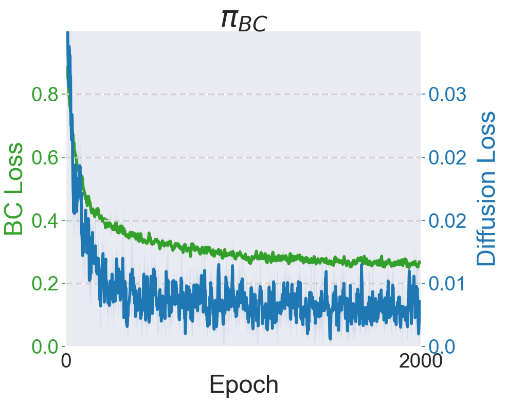
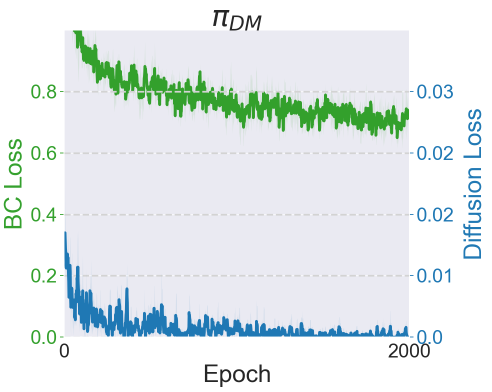
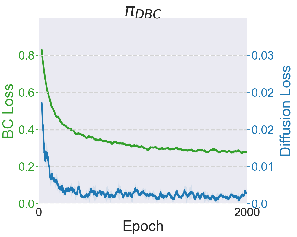
Observing that despite their difference, when $\pi$ converges to $\pi^{E}$, both $\mathcal{L}_{\text{BC}}$ and $\mathcal{L}_{\text{DM}}$ converge to 0, indicating that these two losses are not conflicting. Moreover, our experimental results show that optimizing a combination of these two losses leads to the best performance, compared to solely optimizing each of them.  Table 1 shows that DBC ($\mathcal{L}_{\text{BC}}+\mathcal{L}_{\text{DM}}$) outperforms BC ($\mathcal{L}_{\text{BC}}$) and Table 3 shows that optimizing $\mathcal{L}_{\text{BC}}+\mathcal{L}_{\text{DM}}$ outperforms solely optimizing $\mathcal{L}_{\text{DM}}$.

As shown in  Figure 6, even BC only optimizes $\mathcal{L}_{\text{BC}}$, $\mathcal{L}_{\text{DM}}$ also reduces. However, $\mathcal{L}_{\text{DM}}$ of BC converges to a higher value ($0.0056$), compared to only optimizing $\mathcal{L}_{\text{DM}}$, where $\pi_{DM}$ achieves a $\mathcal{L}_{\text{DM}}$ value of $0.00020$. On the other hand, our proposed DBC can effectively optimize both $\mathcal{L}_{\text{BC}}$ and $\mathcal{L}_{\text{DM}}$, demonstrating the compatibility of the two losses, which justifies the proposed combination of the two losses.

B.2 Relation to F-Divergence

To provide theoretical motivation for our method, we show that optimizing the BC loss can be approximated to optimizing the forward Kullback–Leibler (KL) divergence while optimizing the diffusion model loss can be approximated to optimizing the reverse KL divergence.

First, as shown by Ke et al. [2020], a policy minimizing the KL divergence of the distribution of an expert policy $\pi^{E}$ can be represented as $\hat{\pi}=-\mathbb{E}_{s\sim\rho_{\pi^{E^{\prime}}},a\sim\pi^{E}}[log(\pi(a|s))]$, which is equivalent to the BC objective with the use of a cross-entropy loss. Accordingly, minimizing $\mathcal{L}_{\text{BC}}$ ( Eq. 1) is equal to minimizing the forward KL divergence between the expert distribution and the agent one.

Next, we show how the diffusion model loss can be approximated to optimize the reverse KL divergence in the following. As shown in [J Ho, 2020], the noise prediction objective can optimize the variational bound on negative log probability $\mathbb{E}_{(s,a)\sim D}[-\log\rho_{\pi^{E}}(s,a)]$. In Eq. 3, our diffusion loss $\mathcal{L}_{\text{diff}}^{\text{agent}}$ takes the states $s$ sampled from the dataset $D$ and actions $\hat{a}$ predicted by the policy $\pi$. Therefore, given a pre-trained diffusion model that captures the approximation of expert distribution $\rho_{\pi^{E^{\prime}}}$, we can do the following derivation for the variational bound:

$$\mathbb{E}_{s\sim D,\hat{a}\sim\pi}[-\log\rho_{\pi^{E^{\prime}}}(s,\hat{a})]$$ (7)

$$=\iint[-\rho_{\pi}(s,\hat{a})\log\rho_{\pi^{E^{\prime}}}(s,\hat{a})]\,ds\,d\hat{a}$$

$$=\iint[-\rho_{\pi}(s,\hat{a})\log\rho_{\pi^{E^{\prime}}}(s,\hat{a})+\rho_{\pi}(s,\hat{a})\log\rho_{\pi}(s,\hat{a})-\rho_{\pi}(s,\hat{a})\log\rho_{\pi}(s,\hat{a})]\,ds\,d\hat{a}$$

$$=\iint\rho_{\pi}(s,\hat{a})[\log\rho_{\pi}(s,\hat{a})-\log\rho_{\pi^{E^{\prime}}}(s,\hat{a})]\,ds\,d\hat{a}+\iint-\rho_{\pi}(s,\hat{a})\log\rho_{\pi}(s,\hat{a})\,ds\,d\hat{a}$$

$$=\mathrm{D_{RKL}}(\rho_{\pi^{E^{\prime}}}(s,\hat{a}),\rho_{\pi}(s,\hat{a}))+\mathcal{H}(\rho_{\pi})$$

$$\geq\mathrm{D_{RKL}}(\rho_{\pi^{E^{\prime}}}(s,\hat{a}),\rho_{\pi}(s,\hat{a})),$$

where $\rho_{\pi^{E^{\prime}}}$ and $\rho_{\pi}$ represent the distribution of the estimated expert and the agent state-action pairs respectively, $\mathcal{H}(\rho_{\pi})$ represents the entropy of $\rho_{\pi}$, and $\mathrm{D_{RKL}}(\rho_{\pi^{E^{\prime}}},\rho_{\pi})$ represents the reverse KL divergence of $\rho_{\pi^{E^{\prime}}}$ and $\rho_{\pi}$. As a result, we can minimize the reverse KL divergence between the estimated expert distribution and the agent distribution by optimizing the diffusion loss.

As shown by Ke et al. [2020], the forward KL divergence promotes mode coverage at the cost of occasionally generating poor samples. In contrast, optimizing the reverse KL helps generate high-quality samples at the cost of sacrificing modes. Therefore, these two losses exhibit complementary attributes. Therefore, our DBC combines the BC loss and the proposed diffusion model loss to take advantage of both objectives.

Appendix C Alleviating Manifold Overfitting by Noise Injection

In section Section 5.4, we show that while our diffusion model loss can enhance the generalization ability of the derived policy, the diffusion models may suffer from manifold overfitting during training and, therefore, need to cooperate with the BC objective. Another branch of machine learning research dealing with overfitting problems is noise injection. As shown in Feng et al. [2021], noise injection regularization has shown promising results that resolve the overfitting problem on image generation tasks. In this section, we evaluate if noise injection can resolve the manifold overfitting directly.

C.1 Modeling Expert Distribution

We first verify if noisy injection can help diffusion models capture the expert distribution of the spiral dataset, where the diffusion models fail as shown in Section 5.4. We extensively evaluate diffusion models trained with various levels of noise added to the expert actions. Then, we calculate the average MSE distance between expert actions and the reconstruction of the trained diffusion models, which indicates how well diffusion models capture the expert distribution. We report the result in Table 4.

We observe that applying a noise level of less than 0.02 results in similar MSE distances compared to the result without noise injection (0.0213). The above result indicates that noise injection does not bring an advantage to expert distribution modeling regarding the MSE distance, and the discrepancy between the learned and expert distributions still exists.

Table 4: Expert distribution modeling with diffusion models trained with different noise levels.

Noise level	0	0.002	0.005	0.01	0.02	0.05	0.1
MSE Distance	0.0213	0.0217	0.0248	0.0218	0.0235	0.0330	0.0507

C.2 Guide Policy Learning

In order to examine if the noise-injected diffusion model is better guidance for policy, we further investigate the performance of using the learned diffusion models to guide policy learning. Specifically, we train policies to optimize the diffusion model loss $\mathcal{L}_{\text{DM}}$ provided by either the diffusion model learning from a noise level of 0 or the diffusion model learning from a noise level of 0.01, dubbed $\pi_{\text{DM-0.01}}$.

(a)

(b)

(c)

(d)

Figure 7: Comparing Modeling Conditional Probability and Joint Probability. (a) Expert actions. (b) Expert actions with injected noise. (c) Generated actions by the diffusion model. (d) Rollout trajectories.

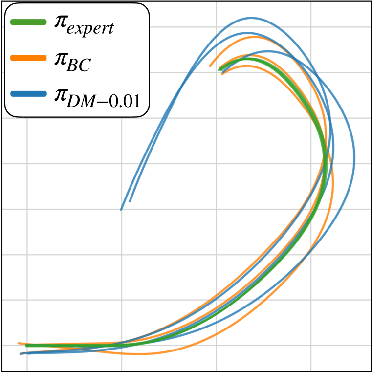
We evaluate the performance of the policies by rolling out each policy and calculating the distance between the end location of the policy and the expert end location. A policy rollout is considered successful if the distance is not greater than 0.1.

In Figure 7, we visualize the expert actions, noise-injected expert actions, generated actions by the diffusion model trained with 0.01 noise level, and the rollout trajectories of the derived policy. The result suggests that the diffusion model learning from expert distribution added with a preferable magnitude noise can better guide policy learning, achieving a success rate of 32%, outperforming the original diffusion model that suffers more from the manifold overfitting with a success rate of 12%. Yet, directly learning to model the conditional probability (i.e., $\pi_{\text{BC}}$) achieves a much higher success rate of 85%. This result verifies the advantage of modeling the conditional probability on this task, which motivates us to incorporate $\mathcal{L}_{\text{BC}}$ in our proposed learning objective instead of solely optimizing $\mathcal{L}_{\text{DM}}$.

Appendix D Comparing to Data Augmentation

To further explore the usage of diffusion models for improving behavioral cloning, we evaluate a straightforward idea: can diffusion models generate informative samples that enhance the performance of BC?

We leverage the diffusion model learning from an expert dataset to generate state-action pairs as a data augmentation method. Specifically, we use 18525 state-action pairs from the Maze dataset to train a diffusion model and then generate 18525 samples with the trained diffusion model. We combine the real and generated state-action pairs and then learn a BC policy. The policy with data augmentation performs 2.06% better than the one without data augmentation, where the improvement is within a standard deviation and lower than our DBC. Therefore, the above results justify the effectiveness of using the diffusion model as a loss source instead of using it for data augmentation.

Appendix E Environment & Task Details

E.1 Maze

Description. A point-maze agent in a 2D maze learns to navigate from its start location to a goal location by iteratively predicting its x and y acceleration. The 6D states include the agent’s two-dimensional current location and velocity, and the goal location. The start and the goal locations are randomized when an episode is initialized.

Evaluation. We evaluate the agents with $100$ episodes and three random seeds and compare our method with the baselines regarding the average success rate and episode lengths, representing the effectiveness and efficiency of the policy learned by different methods. An episode terminates when the maximum episode length of $400$ is reached.

Expert Dataset. The expert dataset consists of the $100$ demonstrations with $18,525$ transitions provided by Lee et al. [2021].

E.2 FetchPick

Description. FetchPick requires a 7-DoF robot arm to pick up an object from the table and move it to a target location. Following the environment setups of Lee et al. [2021], a 16D state representation consists of the angles of the robot joints, the robot arm poses relative to the object, and goal locations. The first three dimensions of the action indicate the desired relative position at the next time step. The fourth dimension of action specifies the distance between the two fingers of the gripper.

Evaluation. We evaluate the agents with $100$ episodes and three random seeds and compare our method with the baselines regarding the average success rate and episode lengths. An episode terminates when the agent completes the task or the maximum episode length is reached, which is set to $50$ for FetchPick.

Expert Dataset. The expert dataset of FetchPick consists of $303$ trajectories ($10k$ transitions) provided by Lee et al. [2021].

E.3 HandRotate

Description. HandRotate Plappert et al. [2018] requires a 24-DoF Shadow Dexterous Hand to in-hand rotate a block to a target orientation. The 68D state representation consists of the joint angles and velocities of the hand, object poses, and the target rotation. The 20D action indicates the position control of the 20 joints, which can be controlled independently. HandRotate is extremely challenging due to its high dimensional state and action spaces. We adapt the experimental setup used in  Plappert et al. [2018] and  Lee et al. [2021], where the rotation is restricted to the z-axis and the possible initial and target z rotations are set within $[-\frac{\pi}{12},\frac{\pi}{12}]$ and $[\frac{\pi}{3},\frac{2\pi}{3}]$, respectively.

Evaluation. We evaluate the agents with $100$ episodes and three random seeds and compare our method with the baselines regarding the average success rate and episode lengths. An episode terminates when the agent completes the goal or the maximum episode length of $50$ is reached.

Expert Dataset. To collect expert demonstrations, we train a SAC Haarnoja et al. [2018] policy using dense rewards for $10M$ environment steps. The dense reward given at each time step $t$ is $R(s_{t},a_{t})=d_{t}-d_{t+1}$, where $d_{t}$ and $d_{t+1}$ represent the angles (in radian) between current and the desired block orientations before and after taking the actions. Following the training stage, the SAC expert policy achieves a success rate of 59.48%. Subsequently, we collect $515$ successful trajectories ($10k$ transitions) from this policy to form our expert dataset for HandRotate.

E.4 Cheetah

Description. The Cheetah is a 2D robot with 17 states, indicating the status of each joint. The goal of this task is to exert torque on the joints to control the robot to walk toward x-direction. The agent would grant positive rewards for forward movement and negative rewards for backward movement.

Evaluation. We evaluate each learned policy with $30$ episodes and three random seeds and compare our method with the baselines regarding the average returns of episodes. The return of an episode is accumulated from all the time steps of an episode. An episode terminates when the agent is unhealthy (i.e., ill conditions predefined in the environment) or the maximum episode length ($1000$) is reached.

Expert Dataset. The expert dataset consists of $5$ trajectories with $5k$ state-action pairs provided by Kostrikov [2018].

E.5 Walker

Description. Walker requires an agent to walk toward x-coordinate as fast as possible while maintaining its balance. The 17D state consists of angles of joints, angular velocities of joints, and velocities of the x and z-coordinate of the top. The 6D action specifies the torques to be applied on each joint of the walker avatar.

Evaluation. We evaluate each learned policy with $30$ episodes and three random seeds and compare our method with the baselines regarding the average returns of episodes. The return of an episode is accumulated from all the time steps of an episode. An episode terminates when the agent is unhealthy (i.e., ill conditions predefined in the environment) or the maximum episode length ($1000$) is reached.

Expert Dataset. The expert dataset consists of $5$ trajectories with $5k$ state-action pairs provided by Kostrikov [2018].

E.6 AntReach

Description.

In the AntReach, the task involves an ant robot with four legs aiming to reach a randomly generated goal on a half-circle with a 5-meter radius centered around the ant. The 42D state includes joint angles, velocities, and the relative position of the goal to the ant.

There is no noise added to the ant’s initial pose during training. However, random noise is introduced during the evaluation, which requires the policies to generalize to unseen states.

The AntReach is a 3D robot with four legs, each consisting of two links. The goal of this task is to control the four legs to move the ant toward the goal.

Evaluation. We evaluate the agents with $100$ episodes and three random seeds and compare our method with the baselines regarding the average success rate and episode lengths. An episode terminates when the agent completes the goal or the maximum episode length of $50$ is reached.

Expert Dataset. The expert dataset comprises 500 trajectories with 25k state-action pairs provided by Lee et al. [2021].

Appendix F Model Architecture

Table 5: Model Architectures. We report the architectures used for all the methods on all the tasks.

Method	Models	Component	Maze	FetchPick	HandRotate	Cheetah	Walker	AntReach
BC	Policy $\pi$	# Layers	4	3	3	3	3	3
		Input Dim.	6	16	68	17	17	42
		Hidden Dim.	256	750	512	256	1024	1024
		Output Dim.	2	4	20	6	6	8
Implicit BC	Policy $\pi$	# Layers	2	2	2	3	2	2
		Input Dim.	8	20	88	23	23	50
		Hidden Dim.	1024	1024	512	512	1024	1200
		Output Dim.	1	1	1	1	1	1
Diffusion Policy	Policy $\pi$	# Layers	5	5	5	5	5	5
		Input Dim.	8	20	88	23	23	42
		Hidden Dim.	256	1200	2100	1200	1200	1200
		Output Dim.	2	4	20	6	6	8
DBC	DM $\phi$	# Layers	5	5	5	5	5	5
		Input Dim.	8	20	88	23	23	50
		Hidden Dim.	128	1024	2048	1024	1024	1024
		Output Dim.	8	20	88	23	23	50
	Policy $\pi$	# Layers	4	3	3	3	3	3
		Input Dim.	6	16	68	17	17	42
		Hidden Dim.	256	750	512	256	1024	1024
		Output Dim.	2	4	20	6	6	8

This section describes the model architectures used for all the experiments. Section F.1 presents the model architectures of BC, Implicit BC, Diffusion Policy, and our proposed framework DBC. Section F.2 details the model architectures of the EBM, VAE, and GAN used for the experiment comparing different generative models.

F.1 Model Architecture of BC, Implicit BC, Diffusion Policy, and DBC

We compare our DBC with three baselines (BC, Implicit BC, and Diffusion Policy) on various tasks in Section 5.3. We detail the model architectures for all the methods on all the tasks in Table 5. Note that all the models, the policy of BC, the energy-based model of Implicit BC, the conditional diffusion model of Diffusion Policy, the policy and the diffusion model of DBC, are parameterized by a multilayer perceptron (MLP). We report the implementation details for each method as follows.

BC. The non-linear activation function is a hyperbolic tangent for all the BC policies. We experiment with BC policies with more parameters, which tend to severely overfit expert datasets, resulting in worse performance.

Implicit BC. The non-linear activation function is ReLU for all energy-based models of Implicit BC. We empirically find that Implicit BC prefers shallow architectures in our tasks, so we set the number of layers to $2$ for the energy-based models.

Diffusion Policy. The non-linear activation function is ReLU for all the policies of Diffusion Policy. We empirically find that Diffusion Policy performs better with a deeper architecture. Therefore, we set the number of layers to $5$ for the policy. In most cases, we use a Diffusion Policy with more parameters than the total parameters of DBC consisting of the policy and the diffusion model.

DBC. The non-linear activation function is ReLU for the diffusion models and is a hyperbolic tangent for the policies. We apply batch normalization and dropout layers with a $0.2$ ratio for the diffusion models on FetchPick.

F.2 Model Architecture of EBM, VAE, and GAN

We compare different generative models (i.e., EBM, VAE, and GAN) on Maze in Section 5.6, and we report the model architectures used for the experiment in this section.

Energy-Based Model. An energy-based model (EBM) consists of $5$ linear layers with ReLU activation. The EBM takes a concatenated state-action pair with a dimension of $8$ as input; the output is a $1$-dimensional vector representing the estimated energy values of the state-action pair. The size of the hidden dimensions is $128$.

Variational Autoencoder. The architecture of a variational autoencoder consists of an encoder and a decoder. The inputs of the encoder are a concatenated state-action pair, and the outputs are the predicted mean and variance, which parameterize a Gaussian distribution. We apply the reparameterization trick [Kingma and Welling, 2014], sample features from the predicted Gaussian distribution, and use the decoder to produce the reconstructed state-action pair. The encoder and the decoder both consist of $5$ linear layers with LeakyReLU Xu et al. [2020] activation. The size of the hidden dimensions is $128$. That said, the encoder maps an $8$-dimensional state-action pair to two $128$-dimensional vectors (i.e., mean and variance), and the decoder maps a sampled $128$-dimensional vector back to an $8$-dimensional reconstructed state-action pair.

Generative Adversarial Network. The architecture of the generative adversarial network consists of a generator and a discriminator. The generator is the policy model that predicts an action from a given state, whose input dimension is $6$ and output dimension is $2$. On the other hand, the discriminator learns to distinguish the expert state-action pairs $(s,a)$ from the state-action pairs produced by the generator $(s,\hat{a})$. Therefore, the input dimension of the discriminator is $8$, and the output is a scalar representing the probability of the state-action pair being "real." The generator and the discriminator both consist of three linear layers with ReLU activation, and the size of the hidden dimensions is $256$.

Appendix G Training and Inference Details

We describe the details of training and performing inference in this section, including computation resources and hyperparameters.

G.1 Computation Resource

We conducted all the experiments on the following three workstations:

• M1: ASUS WS880T workstation with an Intel Xeon W-2255 (10C/20T, 19.25M, 4.5GHz) 48-Lane CPU, 64GB memory, an NVIDIA RTX 3080 Ti GPU, and an NVIDIA RTX 3090 Ti GPU

• M2: ASUS WS880T workstation with an Intel Xeon W-2255 (10C/20T, 19.25M, 4.5GHz) 48-Lane CPU, 64GB memory, an NVIDIA RTX 3080 Ti GPU, and an NVIDIA RTX 3090 Ti GPU

• M3: ASUS WS880T workstation with an Intel Xeon W-2255 (10C/20T, 19.25M, 4.5GHz) 48-Lane CPU, 64GB memory, and two NVIDIA RTX 3080 Ti GPUs

G.2 Hyperparamters

We report the hyperparameters used for all the methods on all the tasks in Table 6. We use the Adam optimizer Kingma and Ba [2015] for all the methods on all the tasks and use linear learning rate decay for all policy models.

Table 6: Hyperparameters. This table reports the hyperparameters used for all the methods on all the tasks. Note that our proposed framework (DBC) consists of two learning modules, the diffusion model and the policy, and therefore their hyperparameters are reported separately.

Method	Hyperparameter	Maze	FetchPick	HandRotate	Cheetah	Walker	AntReach
BC	Learning Rate	5e-5	5e-6	1e-4	1e-4	1e-4	1e-2
	Batch Size	128	128	128	128	128	128
	# Epochs	2000	5000	5000	1000	1000	30000
Implicit BC	Learning Rate	1e-4	5e-6	1e-4	1e-4	1e-4	5e-5
	Batch Size	128	512	128	128	128	128
	# Epochs	10000	15000	15000	10000	10000	30000
Diffusion Policy	Learning Rate	2e-4	1e-5	1e-5	1e-4	1e-4	1e-5
	Batch Size	128	128	128	128	128	128
	# Epochs	20000	15000	30000	10000	10000	30000
DBC (Ours)	Diffusion Model Learning rate	1e-4	1e-3	3e-5	2e-4	2e-4	2e-4
	Diffusion Model Batch Size	128	128	128	128	128	1024
	Diffusion Model # Epochs	8000	10000	10000	8000	8000	20000
	Policy Learning Rate	5e-5	5e-6	1e-4	1e-4	1e-4	0.006
	Policy Batch Size	128	128	128	128	128	128
	Policy # Epochs	2000	5000	5000	1000	1000	10000
	$\lambda$	30	0.1	10	0.2	0.2	1

G.3 Inference Details

This section describes how each method infers an action $\hat{a}$ given a state $s$.

BC & DBC. The policy models of BC and DBC can directly predict an action given a state, i.e., $\hat{a}\sim\pi(s)$, and are therefore more efficient during inference as described in Section 5.3.

Implicit BC. The energy-based model (EBM) of Implicit BC learns to predict an estimated energy value for a state-action pair during training. To generate a predicted $\hat{a}$ given a state $s$ during inference, it requires a procedure to sample and optimize actions. We follow Florence et al. [2022] and implement a derivative-free optimization algorithm to perform inference.

The algorithm first randomly samples $N_{s}$ vectors from the action space as candidates. The EBM then produces the estimated energy value of each candidate action and applies the Softmax function on the estimated energy values to produce a $N_{s}$-dimensional probability. Then, it samples candidate actions according to the above probability and adds noise to them to generate another $N_{s}$ candidates for the next iteration. The above procedure iterates $N_{iter}$ times. Finally, the action with maximum probability in the last iteration is selected as the predicted action $\hat{a}$. In our experiments, $N_{s}$ is set to $1000$ and $N_{iter}$ is set to $3$.

Diffusion Policy. Diffusion Policy learns a conditional diffusion model as a policy and produces an action from sampled noise vectors conditioning on the given state during inference. We follow Pearce et al. [2023], Chi et al. [2023] and adopt Denoising Diffusion Probabilistic Models (DDPMs) J Ho [2020] for the diffusion models. Once learned, the diffusion policy $\pi$ can "denoise" a noise sampled from a Gaussian distribution $\mathcal{N}(0,1)$ given a state $s$ and yield a predicted action $\hat{a}$ using the following equation:

$$a_{n-1}=\frac{1}{\sqrt{\alpha_{n}}}(a_{n}-\frac{1-\alpha_{n}}{\sqrt{1-\bar{\alpha}_{n}}}\pi(s,a_{n},n))+\sigma_{n}z,$$ (8)

where $\alpha_{n}$, $\bar{\alpha}_{n}$, and $\sigma_{n}$ are schedule parameters, $n$ is the current time step of the reverse diffusion process, and $z\sim\mathcal{N}(0,1)$ is a random vector. The above denoising process iterates $N$ times to produce a predicted action $a_{0}$ from a sampled noise $a_{N}\sim\mathcal{N}(0,1)$. The number of total diffusion steps $N$ is $100$ in our experiment, which is the same for the diffusion model in DBC.

G.4 Comparing Different Generative Models

Our proposed framework employs a diffusion model (DM) to model the joint probability of expert state-action pairs and utilizes it to guide policy learning. To justify our choice of generative models, we explore using other popular generative models to replace the diffusion model in Maze. Specifically, we consider energy-based models (EBMs) [Du and Mordatch, 2019, Song and Kingma, 2021], variational autoencoders (VAEs) [Kingma and Welling, 2014], and generative adversarial networks (GANs) Goodfellow et al. [2014]. Each generative model learns to model the joint distribution of expert state-action pairs. For fair comparisons, all the policy models learning from learned generative models consists of $3$ linear layers with ReLU activation, where the hidden dimension is $256$. All the policies are trained for $2000$ epochs using the Adam optimizer [Kingma and Ba, 2015], and a linear learning rate decay is applied for EBMs and VAEs.

G.4.1 Energy-Based Model

Model Learning. Energy-based models (EBMs) learn to model the joint distribution of the expert state-action pairs by predicting an estimated energy value for a state-action pair $(s,a)$. The EBM aims to assign low energy value to the real expert state-action pairs while high energy otherwise. Therefore, the predicted energy value can be used to evaluate how well a state-action pair $(s,a)$ fits the distribution of the expert state-action pair distribution.

To train the EBM, we generate $N_{neg}$ random actions as negative samples for each expert state-action pair as proposed in Florence et al. [2022]. The objective of the EBM $E_{\phi}$ is the InfoNCE loss Oord et al. [2018]:

$$\mathcal{L}_{\text{InfoNCE}}=\frac{e^{-E_{\phi}(s,a)}}{e^{-E_{\phi}(s,a)}+\Sigma_{i=1}^{N_{neg}}e^{-E_{\phi}(s,\tilde{a}_{i})}},$$ (9)

where $(s,a)$ indicates an expert state-action pair, $\tilde{a}_{i}$ indicates the sampled random action, and $N_{neg}$ is set to $64$ in our experiments. The EBM learns to separate the expert state-action pairs from the negative samples by optimizing the above InfoNCE loss.

The EBM is trained for $8000$ epochs with the Adam optimizer [Kingma and Ba, 2015], with a batch size of $128$ and an initial learning rate of $0.0005$. We apply learning rate decay by $0.99$ for every $100$ epoch.

Guiding Policy Learning. To guide a policy $\pi$ to learn, we design an EBM loss $\mathcal{L}_{\text{EBM}}=E_{\phi}(s,\hat{a})$, where $\hat{a}$ indicates the predicted action produced by the policy. The above EBM loss regularizes the policy to generate actions with low energy values, which encourage the predicted state-action pair $(s,\hat{a})$ to fit the modeled expert state-action pair distribution. The policy learning from this EBM loss $\mathcal{L}_{\text{EBM}}$ achieves a success rate of $49.09\%$ in Maze as reported in Table 3.

We also experiment with combining this EBM loss $\mathcal{L}_{\text{EBM}}$ with the $\mathcal{L}_{\text{BC}}$ loss. The policy optimizes $\mathcal{L}_{\text{BC}}+\lambda_{\text{EBM}}\mathcal{L}_{\text{EBM}}$, where $\lambda_{\text{EBM}}$ is set to $0.1$. Optimizing this combined loss yields a success rate of $80.00\%$ in Maze as reported in Table 3.

G.4.2 Variational Autoencoder

Model Learning. Variational autoencoders (VAEs) model the joint distribution of the expert data by learning to reconstruct expert state-action pairs $(s,a)$. Once the VAE is learned, how well a state-action pair fits the expert distribution can be reflected in the reconstruction loss.

The objective of training a VAE is as follows:

$$\mathcal{L}_{\text{vae}}={||\hat{x}-x||}^{2}+D_{\text{KL}}(\mathcal{N}(\mu_{x},\sigma_{x})||\mathcal{N}(0,1)),$$ (10)

where $x$ is the latent variable, i.e., the concatenated state-action pair $x=[s,a]$, and $\hat{x}$ is the reconstruction of $x$, i.e., the reconstructed state-action pair. The first term is the reconstruction loss, while the second term encourages aligning the data distribution with a normal distribution $\mathcal{N}(0,1)$, where $\mu_{x}$ and $\sigma_{x}$ are the predicted mean and standard deviation given $x$.

The VAE is trained for $100k$ update iterations with the Adam optimizer [Kingma and Ba, 2015], with a batch size of $128$ and an initial learning rate of $0.0001$. We apply learning rate decay by $0.5$ for every $5k$ epoch.

Guiding Policy Learning. To guide a policy $\pi$ to learn, we design a VAE loss $\mathcal{L}_{\text{VAE}}=max(\mathcal{L}_{\text{vae}}^{\text{agent}}-\mathcal{L}_{\text{vae}}^{\text{expert}},0)$, similar to Eq. 5. This loss forces the policy to predict an action, together with the state, that can be well reconstructed with the learned VAE. The policy learning from this VAE loss $\mathcal{L}_{\text{VAE}}$ achieves a success rate of $48.47\%$ in Maze as reported in Table 3.

We also experiment with combining this VAE loss $\mathcal{L}_{\text{VAE}}$ with the $\mathcal{L}_{\text{BC}}$ loss. The policy optimizes $\mathcal{L}_{\text{BC}}+\lambda_{\text{VAE}}\mathcal{L}_{\text{VAE}}$, where $\lambda_{\text{VAE}}$ is set to $1$. Optimizing this combined loss yields a success rate of $82.31\%$ in Maze as reported in Table 3.

G.4.3 Generative Adversarial Network

Adversarial Model Learning & Policy Learning. Generative adversarial networks (GANs) model the joint distribution of expert data with a generator and a discriminator. The generator aims to synthesize a predicted action $\hat{a}$ given a state $s$. On the other hand, the discriminator aims to identify expert the state-action pair $(s,a)$ from the predicted one $(s,\hat{a})$. Therefore, a learned discriminator can evaluate how well a state-action pair fits the expert distribution.

While it is possible to learn a GAN separately and utilize the discriminator to guide policy learning, we let the policy $\pi$ be the generator directly and optimize the policy with the discriminator iteratively. We hypothesize that a learned discriminator may be too selective for policy training from scratch, so we learn the policy $\pi$ with the discriminator $D$ to improve the policy and the discriminator simultaneously.

The objective of training the discriminator $D$ is as follows:

$$\mathcal{L}_{\text{disc}}=BCE(D(s,a),1)+BCE(D(s,\hat{a}),0)=-log(D(s,a))-log(1-D(s,\hat{a})),$$ (11)

where $\hat{a}=\pi(s)$ is the predicted action, and $BCE$ is the binary cross entropy loss. The binary label $(0,1)$ indicates whether or not the state-action pair sampled from the expert data. The generator and the discriminator are both updated by Adam optimizers using a $0.00005$ learning rate.

To learn a policy (i.e., generator), we design the following GAN loss:

$$\mathcal{L}_{\text{GAN}}=BCE(D(s,\hat{a}),1)=-log(D(s,\hat{a})).$$ (12)

The above GAN loss guides the policy to generate state-action pairs that fit the joint distribution of the expert data. The policy learning from this GAN loss $\mathcal{L}_{\text{GAN}}$ achieves a success rate of $50.29\%$ in Maze as reported in Table 3.

We also experiment with combining this GAN loss $\mathcal{L}_{\text{GAN}}$ with the $\mathcal{L}_{\text{BC}}$ loss. The policy optimizes $\mathcal{L}_{\text{BC}}+\lambda_{\text{GAN}}\mathcal{L}_{\text{GAN}}$, where $\lambda_{\text{GAN}}$ is set to $0.2$. Optimizing this combined loss yields a success rate of $71.64\%$ in Maze as reported in Table 3.

Appendix H Extended Ablation Study

H.1 Comparing Different Generative Models in FetchPick

Same as in Section 5.6, where we compare using different generative models, including energy-based models (EBMs) [Du and Mordatch, 2019, Song and Kingma, 2021], variational autoencoder (VAEs) [Kingma and Welling, 2014], and generative adversarial networks (GANs) [Goodfellow et al., 2014], to model the expert distribution and guide policy learning in Maze, we conduct the same examination in FetchPick in this subsection.

Table 8 shows that all the generative model-guide policies can be improved by adding the BC loss, justifying our motivation to complement modeling the joint probability with modeling the conditional probability. With BC loss, the diffusion model-guided policy achieves the best performance compared to other generative models, verifying our choice of the generative model. Training details of learning generative models and utilizing them to guide policy learning can be found in Section G.4.

Table 7: Generative Models. We compare using different generative models to model the expert distribution and guide policy learning in FetchPick.

Method	without BC	with BC
BC	N/A	91.6% $\pm$ 5.8%
EBM	5.5% $\pm$ 7.0%	73.7% $\pm$ 14.2%
VAE	0.7% $\pm$ 0.8%	64.2% $\pm$ 6.7%
GAN	41.8% $\pm$ 24.9%	75.0% $\pm$ 9.7%
DM	14.2% $\pm$ 16.2%	97.0% $\pm$ 1.4%

Table 8: Effect of the Normalization Term. To investigate the effectiveness of the normalization term, we evaluate a variant of DBC where only $\mathcal{L}_{\text{diff}}^{\text{agent}}$ in Eq. 3 instead of $\mathcal{L}_{\text{DM}}$ in Eq. 5 is used.

Environment	$\mathcal{L}_{\text{diff}}^{\text{agent}}$	$\mathcal{L}_{\text{DM}}$
Maze	94.7% $\pm$ 1.9%	95.4% $\pm$ 1.7%
FetchPick	96.6% $\pm$ 1.7%	96.9% $\pm$ 1.7%
HandRotate	59.4% $\pm$ 2.1%	60.1% $\pm$ 4.4%
AntReach	77.4% $\pm$ 4.5%	76.5% $\pm$ 3.7%
Cheetah	4821.4 $\pm$ 124.0	4909.5 $\pm$ 73.0
Walker	6976.4 $\pm$ 76.1	7034.6 $\pm$ 33.7

H.2 Comprehensive Experiment on Effect of the Normalization Term

We aim to investigate whether normalizing the diffusion model loss $\mathcal{L}_{\text{DM}}$ with the expert diffusion model loss $\mathcal{L}_{\text{diff}}^{\text{expert}}$ yields improved performance. We train a variant of DBC where only $\mathcal{L}_{\text{diff}}^{\text{agent}}$ in Eq. 3 instead of $\mathcal{L}_{\text{DM}}$ in Eq. 5 is used to augment BC. Comprehensive results in Table 8 show that the performances improve after adding the expert loss normalization term in all of the environments except AntReach, verifying our choice.

Appendix I Qualitative Results and Additional Analysis

This section provides more detailed analyses of our proposed framework and the baselines. We present the qualitative results in Section I.1. Then, we analyze the learning progress of goal-directed tasks during inference in Section I.2.

I.1 Qualitative Results

Rendered videos of the policies learned by our proposed framework and the baselines can be found at https://nturobotlearninglab.github.io/dbc. A screenshot of the rendered videos on the web page is presented in Figure 8.

Figure 8: Qualitative Results. Rendered videos of the policies learned by our proposed framework and the baselines can be found at https://nturobotlearninglab.github.io/dbc.

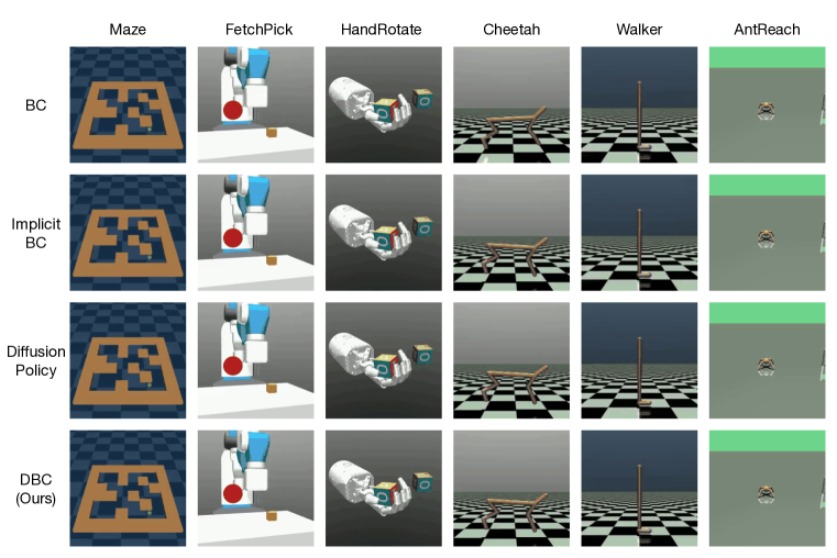
I.2 Learning Progress Analysis

(a) Maze

(b) FetchPick

(c) HandRotate

(d) Cheetah

(e) Walker

(f) AntReach

Figure 9: Learning Progress. We evaluate the baselines and our proposed method DBC and its variants during the learning process. Since Implicit BC (green) and Diffusion Policy (brown) take significantly longer to converge, we set a higher number of training epochs for these two methods, and hence their learning curves are notably longer than BC (orange) and DBC (blue). Our method demonstrates superior learning efficiency over the baselines.

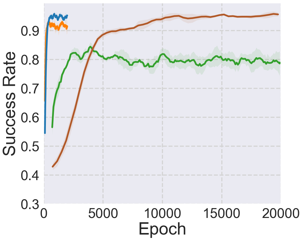
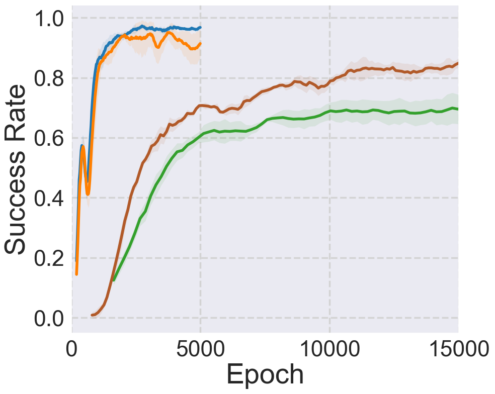
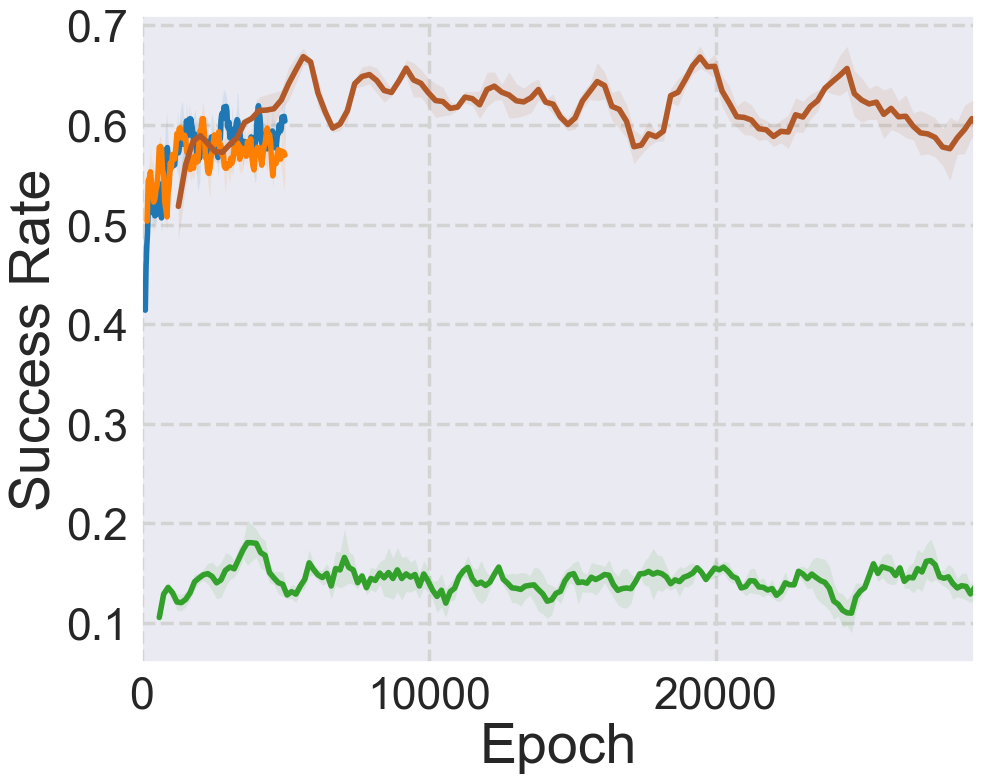
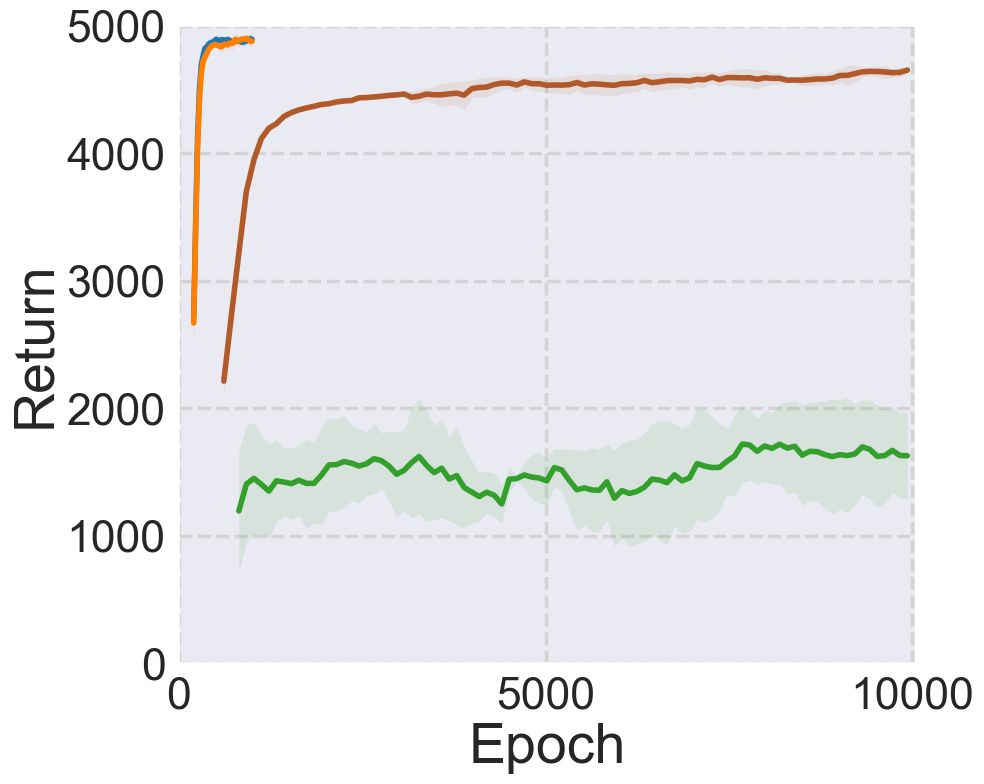
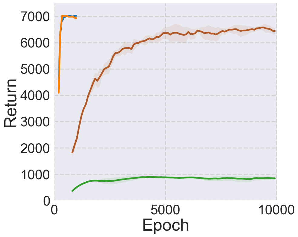
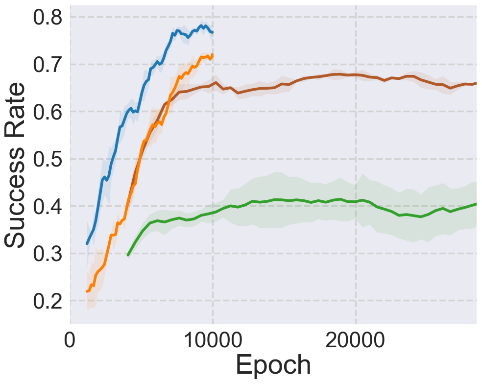
In this section, we analyze the learning progress of all the methods on all the tasks. The training curves are presented in Figure 9. Our proposed framework (DBC) not only achieves the best-converged performance but also converges at a rate comparable to BC, the fast-converging baseline, demonstrating its learning efficiency.

Since Implicit BC and Diffusion Policy take significantly longer to converge, we set a higher number of training epochs for these two methods (see Table 6), and hence their learning curves are notably longer than BC and DBC.

Note that we make sure the numbers of training epochs for Implicit BC and Diffusion Policy are not less than the total number of training epochs for learning both the diffusion model and the policy in DBC. This forecloses the possibility of the superior performance of DBC coming from learning with a higher total number of training epochs.

Appendix J On the Theoretical Motivation for Guiding Policy Learning with Diffusion Model

This section further elaborates on the technical motivation for leveraging diffusion models for imitation learning. Specifically, we aim to learn a diffusion model to model the joint distribution of expert state-action pairs. Then, we propose to utilize this learned diffusion model to augment a BC policy that aims to imitate expert behaviors.

We consider the distribution of expert state-action pairs as the real data distribution $q_{x}$ in learning a diffusion model. Following this setup, $x_{0}$ represents an original expert state-action pair $(s,a)$ and $q(x_{n}|x_{n-1})$ represents the forward diffusion process, which gradually adds Gaussian noise to the data in each timestep $n=1,...,N$ until $x_{N}$ becomes an isotropic gaussian distribution. On the other hand, the reverse diffusion process is defined as $\phi(x_{n-1}|x_{n}):=\mathcal{N}(x_{n-1};\mu_{\theta}(x_{n},n),\Sigma_{\theta}(x_{n},n))$, where $\theta$ denotes the learnable parameters of the diffusion model $\phi$, as illustrated in Figure 1.

Our key idea is to use the proposed diffusion model loss $\mathcal{L}_{\text{DM}}$ in Eq. 5 as an estimate of how well a predicted state-action pair $(s,\hat{a})$ fits the expert state-action pair distribution, as described in Section 4.2.2. In the following derivation, we will show that by optimizing this diffusion model loss $\mathcal{L}_{\text{DM}}$, we maximize the lower bound of the agent data’s probability under the derived expert distribution and hence bring the agent policy $\pi$ closer to the expert policy $\pi^{E}$, which is the goal of imitation learning.

As depicted in  Luo [2022], one can conceptualize diffusion models, including DDPM  [J Ho, 2020] adopted in this work, as a hierarchical variational autoencoder [Kingma and Welling, 2014], which maximizes the likelihood $p(x)$ of observed data points $x$. Therefore, similar to hierarchical variational autoencoders, diffusion models can optimize the Evidence Lower Bound (ELBO) by minimizing the KL divergence $D_{KL}(q(x_{n-1}|x_{n},x_{0})||\phi(x_{n-1}|x_{n}))$. Consequently, this can be viewed as minimizing the KL divergence to fit the distribution of the predicted state-action pairs $(s,\hat{a})$ to the distribution of expert state-action pairs.

According to Bayes’ theorem and the properties of Markov chains, the forward diffusion process $q(x_{n-1}|x_{n},x_{0})$ follows:

$$q(x_{n-1}|x_{n},x_{0})\sim\mathcal{N}(x_{n-1}; \underbrace{\frac{\sqrt{\alpha_{n}}(1-\bar{\alpha}_{n-1})x_{n}+\sqrt{\bar{\alpha}_{n-1}}(1-\alpha_{n})x_{0}}{1-\bar{\alpha_{n}}}}{\mu_{q}(x_{n},x_{0})},$$ (13)

$$\underbrace{\frac{(1-\alpha_{n})(1-\bar{\alpha}_{n-1})}{1-\bar{\alpha}_{n}}}{\Sigma_{q}(n)}).$$

The variation term $\Sigma_{q}(n)$ in the above equation can be written as $\sigma^{2}_{q}(n)I$, where $\sigma^{2}_{q}(n)=\displaystyle\frac{(1-\alpha_{n})(1-\bar{\alpha}_{n-1})}{1-\bar{\alpha}_{n}}$. Therefore, minimizing the KL divergence is equivalent to minimizing the gap between the mean values of the two distributions:

$$\mathop{\arg\min}_{\theta}D_{KL}(q(x_{n-1}|x_{n},x_{0})||\phi(x_{n-1}|x_{n}))$$ (14)

$$=\mathop{\arg\min}_{\theta}D_{KL}(\mathcal{N}(x_{n-1};\mu_{q},\Sigma_{q}(n))||\mathcal{N}(x_{n-1};\mu_{\theta},\Sigma_{q}(n)))$$

$$=\mathop{\arg\min}_{\theta}\frac{1}{2\sigma^{2}_{q}(n)}[||\mu_{\theta}-\mu_{q}||^{2}_{2}],$$

where $\mu_{q}$ represents the denoising transition mean and $\mu_{\theta}$ represents the approximated denoising transition mean by the model.

Different implementations adopt different forms to model $\mu_{\theta}$. Specifically, for DDPMs adopted in this work, the true denoising transition means $\mu_{q}(x_{n},x_{0})$ derived above can be rewritten as:

$$\mu_{q}(x_{n},x_{0})=\frac{1}{\sqrt{\alpha_{n}}}(x_{n}-\frac{1-\alpha_{n}}{\sqrt{1-\bar{\alpha}_{n}}}\epsilon_{0}),$$ (15)

which is referenced from Eq. 11 in J Ho [2020]. Hence, we can set our approximate denoising transition mean $\mu_{\theta}$ in the same form as the true denoising transition mean:

$$\mu_{\theta}(x_{n},n)=\frac{1}{\sqrt{\alpha_{n}}}(x_{n}-\frac{1-\alpha_{n}}{\sqrt{1-\bar{\alpha}_{n}}}\hat{\epsilon_{\theta}}(x_{n},n)),$$ (16)

as illustrated in Popov et al. [2022].  Song et al. [2021] further shows that the entire diffusion model formulation can be revised to view continuous stochastic differential equations (SDEs) as a forward diffusion. It points out that the reverse process is also an SDE, which can be computed by estimating a score function $\nabla_{x}\log p_{t}(x)$ at each denoising time step. The idea of representing a distribution by modeling its score function is introduced in Song and Ermon [2019]. The fundamental concept is to model the gradient of the log probability density function $\nabla_{x}\log p_{t}(x)$, a quantity commonly referred to as the (Stein) score function. Such score-based models are not required to have a tractable normalizing constant and can be directly acquired through score matching. The measure of this score function determines the optimal path to take in the space of the data distribution to maximize the log probability under the derived real distribution.

(a) Maze Layout

(b) Learned Gradient Field

Figure 10: Visualized Gradient Field. (a) Maze Layout: The layout of the medium maze used for Maze. (b) Learned Gradient Field: We visualize the Maze expert demonstration as a distribution of points by their first two dimensions in gray. The points that cluster densely have a high probability, and vice versa. Once a diffusion model is well-trained, it can move randomly sampled points to the area with high probability by predicting gradients (blue arrows). Accordingly, the estimate $p(s,a)$ of joint distribution modeling can serve as guidance for policy learning, as proposed in this work.

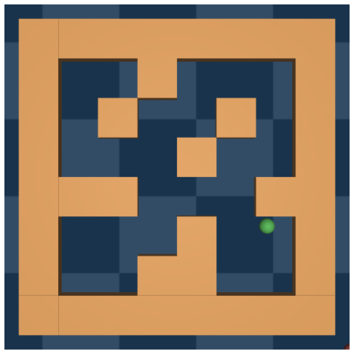
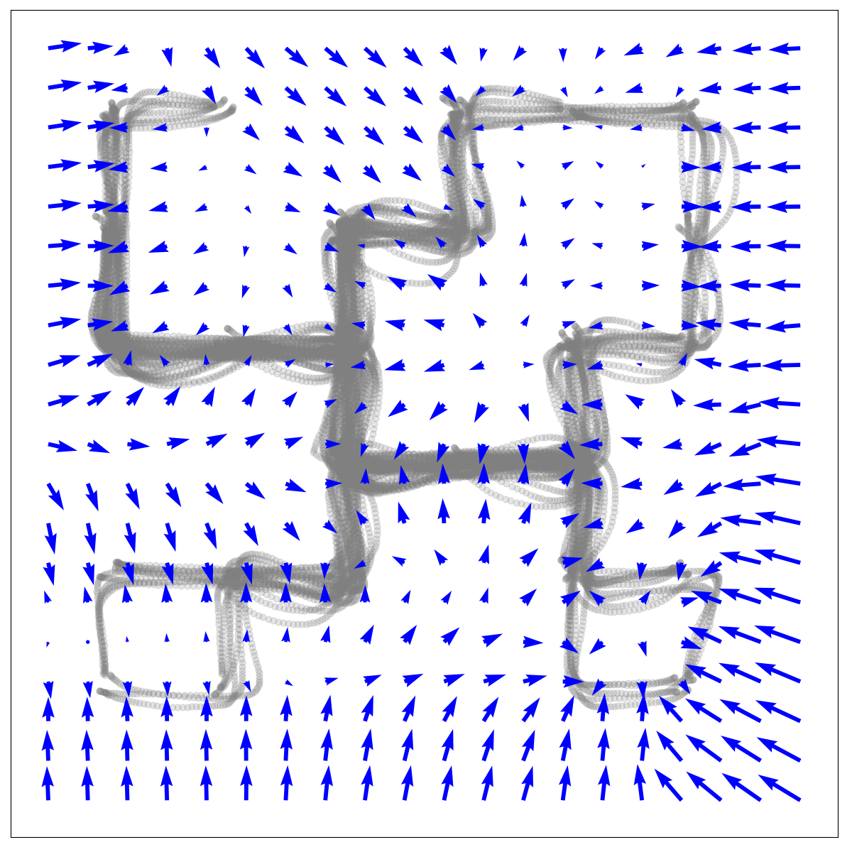
As shown in Figure 10(b), we visualized the learned gradient field of a diffusion model, which learns to model the expert state-action pairs in Maze. Once trained, this diffusion model can guide a policy with predicted gradients (blue arrows) to move to areas with high probability, as proposed in our work.

Essentially, by moving in the opposite direction of the source noise, which is added to a data point $x_{t}$ to corrupt it, the data point is “denoised”; hence the log probability is maximized. This is supported by the fact that modeling the score function is the same as modeling the negative of the source noise. This perspective of the diffusion model is dubbed diffusion SDE. Moreover, Popov et al. [2022] prove that Eq. 16 is diffusion SDE’s maximum likelihood SDE solver. Hence, the corresponding divergence optimization problem can be rewritten as:

$$\mathop{\arg\min}_{\theta}D_{KL}(q(x_{n-1}|x_{n},x_{0})||\phi(x_{n-1}|x_{n}))$$ (17)

$$=\mathop{\arg\min}_{\theta}\frac{1}{2\sigma^{2}_{q}(n)}\frac{(1-\alpha_{n})^{2}}{(1-\bar{\alpha}_{n})\alpha_{n}}[||\hat{\epsilon}_{\theta}(x_{n},n)-\epsilon_{0}||^{2}_{2}],$$

where $\epsilon_{\theta}$ is a function approximator aim to predict $\epsilon$ from $x$. As the coefficients can be omitted during optimization, we yield the learning objective $\mathcal{L}_{\text{diff}}$ as stated in in Eq. 2:

$$\mathcal{L}_{\text{diff}}(s,a,\phi)=\mathbb{E}_{n\sim N,(s,a)\sim D}\{{||\hat{\epsilon}(s,a,n)-\epsilon(n)||}^{2}\}$$ (18)

$$=\mathbb{E}_{n\sim N,(s,a)\sim D}\{{||\phi(s,a,\epsilon(n))-\epsilon(n)||}^{2}\}.$$

The above derivation motivates our proposed framework that augments a BC policy by using the diffusion model to provide guidance that captures the joint probability of expert state-action pairs. Based on the above derivation, minimizing the proposed diffusion model loss (i.e., learning to denoise) is equivalent to finding the optimal path to take in the data space to maximize the log probability. To be more accurate, when the learner policy predicts an action that obtains a lower $\mathcal{L}_{\text{diff}}$, it means that the predicted action $\hat{a}$, together with the given state $s$, fits better with the expert distribution.

Accordingly, by minimizing our proposed diffusion loss, the policy is encouraged to imitate the expert policy. To further alleviate the impact of rarely-seen state-action pairs $(s,a)$, we propose to compute the above diffusion loss for both expert data $(s,a)$ and predicted data $(s,\hat{a})$ and yield $\mathcal{L}_{\text{diff}}^{\text{expert}}$ and $\mathcal{L}_{\text{diff}}^{\text{agent}}$, respectively. Therefore, we propose to augment BC with this objective: $\mathcal{L}_{\text{DM}}=\mathbb{E}_{(s,a)\sim D,\hat{a}\sim\pi(s)}\{max(\mathcal{L}_{\text{diff}}^{\text{agent}}-\mathcal{L}_{\text{diff}}^{\text{expert}},0)\}.$

Appendix K Limitations

This section discusses the limitations of our proposed framework.

• Since this work aims to learn from demonstrations without interacting with environments, our proposed framework in its current form is only designed to learn from expert trajectories and cannot learn from trajectories produced by the learner policy. Extending our method to incorporate agent data can potentially allow for improvement when interacting environments are possible, which is left for future work.

• The key insight of our work is to allow the learner policy to benefit from both modeling the conditional and joint probability of expert state-action distributions. To this end, we propose to optimize both the BC loss and the proposed diffusion model loss. To balance the importance of the two losses, we introduce a coefficient $\lambda$ as an additional hyperparameter. While the ablation study conducted in Maze shows that the performance of our proposed framework is robust to $\lambda$, this can potentially increase the difficulty of searching for optimal hyperparameters when applying our proposed framework to a new application.

Table 9: Maze Dataset Size Experimental Result. We report the mean and the standard deviation of the success rate of different dataset sizes of Maze. The results show that our proposed method DBC performs competitively against the Diffusion Policy and outperforms the other baselines across different dataset sizes.

Method	Dataset Size
	25%	50%	75%	100%
BC	49.8% $\pm$ 4.6%	71.9% $\pm$ 4.9%	81.7% $\pm$ 5.2%	92.1% $\pm$ 3.6%
Implicit BC	51.9% $\pm$ 3.7%	65.9% $\pm$ 5.1%	71.1% $\pm$ 5.0%	78.3% $\pm$ 6.0%
Diffusion Policy	72.7% $\pm$ 9.2%	83.7% $\pm$ 3.1%	88.4% $\pm$ 4.5%	95.5% $\pm$ 1.9%
DBC (Ours)	71.2% $\pm$ 3.9%	83.9% $\pm$ 3.2%	93.1% $\pm$ 2.6%	95.4% $\pm$ 1.7%

Appendix L Broader Impacts

This work proposes Diffusion Model-Augmented Behavioral Cloning, a novel imitation learning framework that aims to increase the ability of autonomous learning agents (e.g., robots, game AI agents) to acquire skills by imitating demonstrations provided by experts (e.g., humans). However, it is crucial to acknowledge that our proposed framework, by design, inherits any biases exhibited by the expert demonstrators. These biases can manifest as sub-optimal, unsafe, or even discriminatory behaviors. To address this concern, ongoing research endeavors to mitigate bias and promote fairness in machine learning hold promise in alleviating these issues. Moreover, research works that enhance learning agents’ ability to imitate experts, such as this work, can pose a threat to job security. Nevertheless, in sum, we firmly believe that our proposed framework can offer tremendous advantages in terms of enhancing the quality of human life and automating laborious, arduous, or perilous tasks that pose risks to humans, which far outweigh the challenges and potential issues.

Appendix M Dataset Size

We conducted experiments in the Maze environment using 0.25, 0.5, and 0.75 fractions of the original dataset size. We used the same set of hyperparameters for each method as reported in Section G.2. The results in Table 9 show that our proposed method DBC performs competitively against the Diffusion Policy and outperforms the other baselines across different dataset sizes. The BC baseline demonstrates a noticeable drop in performance as the dataset size decreases, and the Implicit BC baseline consistently exhibits inferior performance as the dataset size decreases. The results demonstrate that our proposed framework and Diffusion Policy exhibit greater robustness to dataset size compared to BC and Implicit BC.

References

- Mnih et al. [2015] Volodymyr Mnih, Koray Kavukcuoglu, David Silver, Andrei A Rusu, Joel Veness, Marc G Bellemare, Alex Graves, Martin Riedmiller, Andreas K Fidjeland, Georg Ostrovski, et al. Human-level control through deep reinforcement learning. Nature, 2015.
- Lillicrap et al. [2016] Timothy P. Lillicrap, Jonathan J. Hunt, Alexander Pritzel, Nicolas Heess, Tom Erez, Yuval Tassa, David Silver, and Daan Wierstra. Continuous control with deep reinforcement learning. In International Conference on Learning Representations, 2016.
- Arulkumaran et al. [2017] Kai Arulkumaran, Marc Peter Deisenroth, Miles Brundage, and Anil Anthony Bharath. Deep reinforcement learning: A brief survey. IEEE Signal Processing Magazine, 2017.
- Christiano et al. [2017] Paul F Christiano, Jan Leike, Tom Brown, Miljan Martic, Shane Legg, and Dario Amodei. Deep reinforcement learning from human preferences. In Advances in Neural Information Processing Systems, 2017.
- Leike et al. [2018] Jan Leike, David Krueger, Tom Everitt, Miljan Martic, Vishal Maini, and Shane Legg. Scalable agent alignment via reward modeling: a research direction. arXiv preprint arXiv:1811.07871, 2018.
- Lee et al. [2019] Youngwoon Lee, Shao-Hua Sun, Sriram Somasundaram, Edward S. Hu, and Joseph J. Lim. Composing complex skills by learning transition policies. In Proceedings of International Conference on Learning Representations, 2019.
- Garcıa and Fernández [2015] Javier Garcıa and Fernando Fernández. A comprehensive survey on safe reinforcement learning. Journal of Machine Learning Research, 2015.
- Levine et al. [2020] Sergey Levine, Aviral Kumar, George Tucker, and Justin Fu. Offline reinforcement learning: Tutorial, review, and perspectives on open problems. arXiv preprint arXiv:2005.01643, 2020.
- Schaal [1997] Stefan Schaal. Learning from demonstration. In Advances in Neural Information Processing Systems, 1997.
- Osa et al. [2018] Takayuki Osa, Joni Pajarinen, Gerhard Neumann, J Andrew Bagnell, Pieter Abbeel, Jan Peters, et al. An algorithmic perspective on imitation learning. Foundations and Trends® in Robotics, 2018.
- Ho and Ermon [2016] Jonathan Ho and Stefano Ermon. Generative adversarial imitation learning. In Advances in Neural Information Processing Systems, 2016.
- Zolna et al. [2021] Konrad Zolna, Scott Reed, Alexander Novikov, Sergio Gomez Colmenarejo, David Budden, Serkan Cabi, Misha Denil, Nando de Freitas, and Ziyu Wang. Task-relevant adversarial imitation learning. In Conference on Robot Learning, 2021.
- Kostrikov et al. [2019] Ilya Kostrikov, Kumar Krishna Agrawal, Debidatta Dwibedi, Sergey Levine, and Jonathan Tompson. Discriminator-actor-critic: Addressing sample inefficiency and reward bias in adversarial imitation learning. In International Conference on Learning Representations, 2019.
- Ng and Russell [2000] Andrew Y. Ng and Stuart J. Russell. Algorithms for inverse reinforcement learning. In International Conference on Machine Learning, 2000.
- Abbeel and Ng [2004] Pieter Abbeel and Andrew Y Ng. Apprenticeship learning via inverse reinforcement learning. In International Conference on Machine Learning, 2004.
- Pomerleau [1989] Dean A Pomerleau. Alvinn: An autonomous land vehicle in a neural network. In Advances in Neural Information Processing Systems, 1989.
- Bain and Sammut [1995] Michael Bain and Claude Sammut. A framework for behavioural cloning. In Machine Intelligence 15, 1995.
- Nguyen et al. [2023] Tung Nguyen, Qinqing Zheng, and Aditya Grover. Reliable conditioning of behavioral cloning for offline reinforcement learning. arXiv preprint arXiv:2210.05158, 2023.
- Bishop and Nasrabadi [2006] Christopher M Bishop and Nasser M Nasrabadi. Pattern recognition and machine learning. Springer, 2006.
- Fisch et al. [2013] Dominik Fisch, Edgar Kalkowski, and Bernhard Sick. Knowledge fusion for probabilistic generative classifiers with data mining applications. IEEE Transactions on Knowledge and Data Engineering, 2013.
- Wu et al. [2021] Qitian Wu, Rui Gao, and Hongyuan Zha. Bridging explicit and implicit deep generative models via neural stein estimators. In Neural Information Processing Systems, 2021.
- Loaiza-Ganem et al. [2022] Gabriel Loaiza-Ganem, Brendan Leigh Ross, Jesse C Cresswell, and Anthony L Caterini. Diagnosing and fixing manifold overfitting in deep generative models. Transactions on Machine Learning Research, 2022.
- Zhao et al. [2023] Tony Z Zhao, Vikash Kumar, Sergey Levine, and Chelsea Finn. Learning fine-grained bimanual manipulation with low-cost hardware. arXiv preprint arXiv:2304.13705, 2023.
- Ly and Akhloufi [2020] Abdoulaye O Ly and Moulay Akhloufi. Learning to drive by imitation: An overview of deep behavior cloning methods. IEEE Transactions on Intelligent Vehicles, 2020.
- Harmer et al. [2018] Jack Harmer, Linus Gisslén, Jorge del Val, Henrik Holst, Joakim Bergdahl, Tom Olsson, Kristoffer Sjöö, and Magnus Nordin. Imitation learning with concurrent actions in 3d games. In IEEE Conference on Computational Intelligence and Games, 2018.
- Torabi et al. [2018] Faraz Torabi, Garrett Warnell, and Peter Stone. Behavioral cloning from observation. In International Joint Conference on Artificial Intelligence, 2018.
- Ross et al. [2011] Stéphane Ross, Geoffrey Gordon, and Drew Bagnell. A reduction of imitation learning and structured prediction to no-regret online learning. In International Conference on Artificial Intelligence and Statistics, 2011.
- Florence et al. [2022] Pete Florence, Corey Lynch, Andy Zeng, Oscar A Ramirez, Ayzaan Wahid, Laura Downs, Adrian Wong, Johnny Lee, Igor Mordatch, and Jonathan Tompson. Implicit behavioral cloning. In Conference on Robot Learning, 2022.
- Torabi et al. [2019] Faraz Torabi, Garrett Warnell, and Peter Stone. Generative adversarial imitation from observation. In International Conference on Machine Learning, 2019.
- Jena et al. [2021] Rohit Jena, Changliu Liu, and Katia Sycara. Augmenting gail with bc for sample efficient imitation learning. In Conference on Robot Learning, pages 80–90. PMLR, 2021.
- Goodfellow et al. [2014] Ian Goodfellow, Jean Pouget-Abadie, Mehdi Mirza, Bing Xu, David Warde-Farley, Sherjil Ozair, Aaron Courville, and Yoshua Bengio. Generative adversarial nets. In Advances in Neural Information Processing Systems, 2014.
- Chen et al. [2020] Minshuo Chen, Yizhou Wang, Tianyi Liu, Zhuoran Yang, Xingguo Li, Zhaoran Wang, and Tuo Zhao. On computation and generalization of generative adversarial imitation learning. In International Conference on Learning Representations, 2020.
- Fu et al. [2018] Justin Fu, Katie Luo, and Sergey Levine. Learning robust rewards with adverserial inverse reinforcement learning. In International Conference on Learning Representations, 2018.
- Lee et al. [2021] Youngwoon Lee, Andrew Szot, Shao-Hua Sun, and Joseph J. Lim. Generalizable imitation learning from observation via inferring goal proximity. In Neural Information Processing Systems, 2021.
- Pearce et al. [2023] Tim Pearce, Tabish Rashid, Anssi Kanervisto, David Bignell, Mingfei Sun, Raluca Georgescu, Sergio Valcarcel Macua, Shan Zheng Tan, Ida Momennejad, Katja Hofmann, and Sam Devlin. Imitating human behaviour with diffusion models. In International Conference on Learning Representations, 2023.
- Chi et al. [2023] Cheng Chi, Siyuan Feng, Yilun Du, Zhenjia Xu, Eric Cousineau, Benjamin Burchfiel, and Shuran Song. Diffusion policy: Visuomotor policy learning via action diffusion. In Robotics: Science and Systems, 2023.
- Reuss et al. [2023] Moritz Reuss, Maximilian Li, Xiaogang Jia, and Rudolf Lioutikov. Goal-conditioned imitation learning using score-based diffusion policies. arXiv preprint arXiv:2304.02532, 2023.
- Codevilla et al. [2019] Felipe Codevilla, Eder Santana, Antonio M López, and Adrien Gaidon. Exploring the limitations of behavior cloning for autonomous driving. In International Conference on Computer Vision, 2019.
- Wang et al. [2022] Lingguang Wang, Carlos Fernandez, and Christoph Stiller. High-level decision making for automated highway driving via behavior cloning. IEEE Transactions on Intelligent Vehicles, 2022.
- Ganapathi et al. [2022] Aditya Ganapathi, Pete Florence, Jake Varley, Kaylee Burns, Ken Goldberg, and Andy Zeng. Implicit kinematic policies: Unifying joint and cartesian action spaces in end-to-end robot learning. In International Conference on Robotics and Automation, 2022.
- Du and Mordatch [2019] Yilun Du and Igor Mordatch. Implicit generation and modeling with energy based models. In Neural Information Processing Systems, 2019.
- Song and Kingma [2021] Yang Song and Diederik P Kingma. How to train your energy-based models. arXiv preprint arXiv:2101.03288, 2021.
- Kingma and Welling [2014] Diederik P Kingma and Max Welling. Auto-encoding variational bayes. In International Conference on Learning Representations, 2014.
- Rezende and Mohamed [2015] Danilo Rezende and Shakir Mohamed. Variational inference with normalizing flows. In International Conference on Machine Learning, 2015.
- Dinh et al. [2017] Laurent Dinh, Jascha Sohl-Dickstein, and Samy Bengio. Density estimation using real NVP. In International Conference on Learning Representations, 2017.
- Sohl-Dickstein et al. [2015] Jascha Sohl-Dickstein, Eric Weiss, Niru Maheswaranathan, and Surya Ganguli. Deep unsupervised learning using nonequilibrium thermodynamics. In International Conference on Machine Learning, 2015.
- Nichol and Dhariwal [2021] Alexander Quinn Nichol and Prafulla Dhariwal. Improved denoising diffusion probabilistic models. In International Conference on Machine Learning, 2021.
- Dhariwal and Nichol [2021] Prafulla Dhariwal and Alexander Nichol. Diffusion models beat gans on image synthesis. In Neural Information Processing Systems, 2021.
- Ko et al. [2023] Po-Chen Ko, Jiayuan Mao, Yilun Du, Shao-Hua Sun, and Joshua B. Tenenbaum. Learning to act from actionless videos through dense correspondences. arXiv preprint arXiv:2310.08576, 2023.
- J Ho [2020] A Jain J Ho. Denoising diffusion probabilistic models. In Advances in Neural Information Processing Systems, 2020.
- Fu et al. [2020] Justin Fu, Aviral Kumar, Ofir Nachum, George Tucker, and Sergey Levine. D4rl: Datasets for deep data-driven reinforcement learning. arXiv preprint arXiv:2004.07219, 2020.
- Plappert et al. [2018] Matthias Plappert, Marcin Andrychowicz, Alex Ray, Bob McGrew, Bowen Baker, Glenn Powell, Jonas Schneider, Josh Tobin, Maciek Chociej, Peter Welinder, et al. Multi-goal reinforcement learning: Challenging robotics environments and request for research. arXiv preprint arXiv:1802.09464, 2018.
- Haarnoja et al. [2018] Tuomas Haarnoja, Aurick Zhou, Pieter Abbeel, and Sergey Levine. Soft actor-critic: Off-policy maximum entropy deep reinforcement learning with a stochastic actor. In Proceedings of International Conference on Machine Learning, 2018.
- Brockman et al. [2016] Greg Brockman, Vicki Cheung, Ludwig Pettersson, Jonas Schneider, John Schulman, Jie Tang, and Wojciech Zaremba. Openai gym, 2016.
- Kostrikov [2018] Ilya Kostrikov. Pytorch implementations of reinforcement learning algorithms. https://github.com/ikostrikov/pytorch-a2c-ppo-acktr-gail, 2018.
- Ke et al. [2020] Liyiming Ke, Sanjiban Choudhury, Matt Barnes, Wen Sun, Gilwoo Lee, and Siddhartha Srinivasa. Imitation learning as f-divergence minimization. In International Workshop on the Algorithmic Foundations of Robotics, 2020.
- Feng et al. [2021] Ruili Feng, Deli Zhao, and Zheng-Jun Zha. Understanding noise injection in gans. In international conference on machine learning, pages 3284–3293. PMLR, 2021.
- Xu et al. [2020] Jin Xu, Zishan Li, Bowen Du, Miaomiao Zhang, and Jing Liu. Reluplex made more practical: Leaky relu. In IEEE Symposium on Computers and Communications, 2020.
- Kingma and Ba [2015] Diederik P Kingma and Jimmy Ba. Adam: A method for stochastic optimization. In Proceedings of International Conference on Learning Representations, 2015.
- Oord et al. [2018] Aaron van den Oord, Yazhe Li, and Oriol Vinyals. Representation learning with contrastive predictive coding. arXiv preprint arXiv:1807.03748, 2018.
- Luo [2022] Calvin Luo. Understanding diffusion models: A unified perspective. arXiv preprint arXiv:2208.11970, 2022.
- Popov et al. [2022] Vadim Popov, Ivan Vovk, Vladimir Gogoryan, Tasnima Sadekova, Mikhail Kudinov, and Jiansheng Wei. Diffusion-based voice conversion with fast maximum likelihood sampling scheme. In International Conference on Learning Representations, 2022.
- Song et al. [2021] Yang Song, Jascha Sohl-Dickstein, Diederik P Kingma, Abhishek Kumar, Stefano Ermon, and Ben Poole. Score-based generative modeling through stochastic differential equations. In International Conference on Learning Representations, 2021.
- Song and Ermon [2019] Yang Song and Stefano Ermon. Generative modeling by estimating gradients of the data distribution. In Neural Information Processing Systems, 2019.