Vacuum Entanglement Harvesting in the Ising Model

Abstract

The low-energy states of quantum many body systems, such as spin chains, are entangled. Using tensor network computations, we demonstrate a protocol that distills Bell pairs out of the ground state of the prototypical transverse-field Ising model. We explore the behavior of rate of entanglement distillation in various phases, and possible optimizations of the protocol. Finally, we comment on the protocol as we approach quantum criticality defining a continuum field theory.

I Introduction

Continuum quantum field theories (qfts) are the cornerstone for our current understanding of the standard model of particle physics. Motivated by experiments, traditional studies of qfts had focused on calculating the phases of ground states through local order parameters, spectral quantities of low lying excitations, interaction coupling constants, etc. More recently, there has been considerable interest in understanding the connection of qfts to quantum information science. This has motivated physicists to consider entanglement properties of qft [1]. While it has been known for a long time that bounded energy states of qfts display long-distance entanglement [2, 3, 4, 5, 6, 7, 8, 9, 10], recently the focus has turned to understanding the entanglement in interacting quantum many body systems [11, *[Seereview][andreferencestherein.]RevModPhys.80.517]. The nature [13, 14] and the dynamics [15, 16] of this entanglement has been extensively studied in a limited class of systems. Entanglement properties of ground states can also help identify new types of phases of matter, based on topological order that are difficult to understand using local order parameters [17]. Entanglement has also been shown to be key to understanding the success of tensor network algorithms for quantum many body systems [18].

While entanglement structure has been well established to be important in gaining insight into quantum systems with extensive degrees of freedom, such as qfts, one can ask whether this entanglement can be used to carry out useful tasks? Many quantum information protocols, such as communication [19] and teleportation [20], rely on a supply of entangled Bell pairs. The idea of extracting Bell pairs from the vacuum of a qft was pioneered in Refs. [21, 22, 23, 24]. In particular, these early works demonstrated that two qubits can be entangled by coupling them to quantum fields, even in a spacelike separated region of spacetime. Further works have analyzed entanglement harvesting from thermal states [25, 26, 27], from coherent scalar field states [28], and from the electromagnetic vacuum using hydrogen-like atoms [29]; and investigated dependence of entanglement harvesting on switching protocols [30], on the detector gaps in relation to the mass of the field [31], on other detector properties [30, 32, 33] and on the spacetime structure [34, 35].

While these studies have demonstrated the entanglement in physical states of qfts can indeed be exploited for quantum information tasks [21, 24, 23, 22], they are formulated in the continuum and most limit themselves to perturbation theory. For a fundamental understanding of the phenomena and for wider applicability, a nonperturbative analysis is desirable. A powerful tool to study nonperturbative aspects of qft is the use of lattice field theory, where the qft is seen as the description of the long-distance limit of a quantum theory defined on a discrete spacetime (or spatial) lattice at its quantum critical point. Currently, the only way to do computations with 4d lattice field theory is with Monte Carlo (mc) methods, but the inherent nonequilibrium nature of the entanglement harvesting protocols means that even the lattice mc methods fail with severe sign problems. An alternative approach to conventional lattice field theory and its simulation is needed.

In this work, we take a first step towards a nonperturbative study of entanglement harvesting in qft using lattice field theory. The question we are interested in this work is: can one distill Bell pairs out of the ground state of a relativistic qft, and, if so, at what rate? In other words, how can two parties—conventionally called Alice and Bob—do cooperative quantum tasks using the vacuum? As discussed above, this is a difficult question to probe quantitatively directly in the continuum for relativistic qfts. However, in low dimensions, the quantum systems whose second-order critical points are described by the continuum qfts allow the use of tensor network techniques in a study of entanglement and their real-time dynamics. More specifically, we focus on one of the simplest lattice field theories, the one-dimensional Transverse Field Ising Model (tfim), and analyze a simple protocol for the distillation of Bell pairs out of the ground state (or vacuum) of the theory using tensor networks.

The number of entangled Bell pairs which can be extracted from a system can be thought of as a measure of entanglement, called the “entanglement of distillation” [36], which is however difficult to compute. It has been shown that entanglement negativity [37] gives an upper bound to distillable entanglement, and thus can be a useful proxy for it. Gaussian states have been used to compute negativities in free (bosonic and fermionic) lattice field theories [38, 39, 40, 41, 42] and study their continuum limits [43, 44, 45]. However, these methods do not work for interacting field theories. In 1+1 dimensions, conformal field theory (cft) methods have been used to compute negativities [46, 41, 47, 48, 49, 42], and even the realtime dynamics after local quenches in some cases [50, 51, 52]. However, the computation of the negativity between two finite and disjoint intervals, which is the one relevant to us, is still difficult in general.

On the other hand, given a quantum state represented as a matrix product states (mps), the entanglement negativity between two disjoint regions can be computed efficiently. Therefore, for low-dimensional (1d or 2d) systems, tensor networks provide a powerful method for computing entanglement negativity, which we exploit in this work.

This paper is organized as follows. In Section II, we provide a brief pedagogical summary of the basic concepts related to entanglement negativity and entanglement harvesting. In Section III, we define entanglement negativity of the ground state of the tfim and investigate its behavior across the phase transition. In Section IV, we introduce a simple protocol for entanglement harvesting from a quantum spin chain and study the protocol in the thermodynamic limit, and describe our results for the tfim. We present our conclusions in Section V. We explain a few technical details in the appendices. Appendix A is a pedagogical introduction to the use of reduced density matrices to single quantum systems; Appendix B analyzes the role of permutation symmetry in studying density matrices describing systems drawn from an ensemble; and Appendix C discusses the use of reduced density matrices for a thermodynamic system where ergodicity is broken. Appendix D describes the mps ansatz and its implementation in our work, and in Appendix E, results from some exact calculations are compared against those obtained using the Density Matrix Renormalization Group (dmrg). Finally, Appendix F describes our parameterization of maximally entangled 2-qubit states.

II Entanglement Negativity

There are several quantities in quantum mechanics that allow us to assess the quantum nature of the physical system. The most well known example is entanglement. If we consider some quantum system $S$ in a pure state, but focus only on some subsystem $A$ so that we only have access to information within $A$, then we can learn how $A$ is entangled with $S$ through the reduced density matrix $\rho^{\rm r}_{A}$. For example, the von Neumann entropy

$$S_{A}\ =\ -\mathrm{Tr}_{A}\left(\rho^{\rm r}_{A}\ln\rho^{\rm r}_{A}\right),$$ (1)

is nonzero if $A$ is entangled with the remaining system and, thus, contrary to classical expectations, we will find $A$ to be in a mixed state, even though the density matrix $\rho$ of the full system $S$ describing a pure state has vanishing von Neumann entropy.

If instead of a single subsystem we consider two subsystems $A$ and $B$ inside some bigger quantum system $S$, the situation is more complex. As before, let us assume the full system $S$ is in some pure state so that the density matrix $\rho$ of the full system has a vanishing von Neumann entropy. For a generic quantum many body state, the combined subsystem $A$ and $B$ will be in a mixed state and entangled with the rest of the system. This means that reduced density matrix $\rho^{\rm r}_{AB}$ will, in general, be characterized by a nonzero von Neumann entropy. For such mixed states, the easiest way to detect entanglement between $A$ and $B$ is by using an “entanglement witness,” an operator that is positive semidefinite when restricted to unentangled states, but not in general. (See Ref. [36] and references therein.) One such class of operators arises from the positive maps on one subsystem (say $A$) but that are not positive on the entire system when combined with the identity operation on the other subsystem. These are called positive but not completely positive maps.

A convenient entanglement witness in this class is the hermiticity and trace-preserving ‘partial transpose’ [53]. It is easiest to define this operator using a direct-product basis for the joint state of the subsystems $A$ and $B$, i.e., a basis using states $\mathclose{\,\mathopen{|}\mathord{ab}\mathclose{\rangle}}\equiv{\mathclose{\,\mathopen{|}\mathord{a}\mathclose{\rangle}}}_{A}\otimes{\mathclose{\,\mathopen{|}\mathord{b}\mathclose{\rangle}}}_{B}$, built out of any orthonormal basis, $\{{\mathclose{\,\mathopen{|}\mathord{a}\mathclose{\rangle}}}_{A}\}$ and $\{{\mathclose{\,\mathopen{|}\mathord{b}\mathclose{\rangle}}}_{B}\}$, for the Hilbert spaces of subsystems $A$ and $B$ respectively. Then we can express the reduced density in terms of its components $\rho^{ab}_{a^{\prime}b^{\prime}}$ as

$$\rho_{AB} \equiv\sum_{\begin{subarray}{c}a,b\\ a^{\prime},b^{\prime}\end{subarray}}\rho^{ab}_{a^{\prime}b^{\prime}}\mathclose{\,\mathopen{|}\mathord{ab}\mathclose{\rangle}}\mathopen{\mathopen{\langle}\mathord{a^{\prime}b^{\prime}}\mathclose{|}\,},$$ (2)

which is clearly an operator in the direct product space of $A$ and $B$. The hermiticity, positivity, and trace-preserving ‘partial transpose’ operator can then be defined as $(T_{A}\otimes I_{B})$ whose action on $\rho_{AB}$ is defined as

$$\rho_{AB}^{T_{A}}\equiv(T_{A}\otimes\mathbb{I}_{B})\ \rho_{AB}\equiv\sum_{\begin{subarray}{c}a,b\\ a^{\prime},b^{\prime}\end{subarray}}\rho^{a^{\prime}b}_{ab^{\prime}}\mathclose{\,\mathopen{|}\mathord{ab}\mathclose{\rangle}}\mathopen{\mathopen{\langle}\mathord{a^{\prime}b^{\prime}}\mathclose{|}\,}\,.$$ (3)

Note that though the partial transpose operation depends on the basis chosen, the operations defined with respect to different orthonormal bases for each of the subsystems are all unitarily equivalent, and so $\rho_{AB}^{T_{A}}$ has the same eigenvalue spectrum in all bases. In particular the trace norm

$$\mathopen{||}\rho^{T_{A}}_{AB}\mathclose{||}_{1}\equiv\operatorname{Tr}\sqrt{(\rho^{T_{A}}_{AB})^{\dagger}\rho^{T_{A}}_{AB}}$$ (4)

is basis independent. Further, it is easy to verify that $\mathopen{||}\rho^{T_{B}}_{AB}\mathclose{||}_{1}=\mathopen{||}\rho^{T_{A}}_{AB}\mathclose{||}_{1}$.

Entanglement negativity ${\cal N}(\rho_{AB})$ between two subsystems $A$ and $B$ characterized by the density matrix $\rho_{AB}$ is then defined as the sum over all negative eigenvalues of $\rho_{AB}^{T_{A}}$ [37], which can be conveniently computed through the relation

$${\cal N}(\rho_{AB})\equiv\frac{\mathopen{||}\rho^{T_{A}}_{AB}\mathclose{||}_{1}-1}{2}.$$ (5)

The logarithmic negativity is then defined through the relation

$$E_{N}(\rho)\equiv\log_{2}(\mathopen{||}\rho^{T_{A}}\mathclose{||}_{1})=\log_{2}(2{\cal N}+1).$$ (6)

Any density matrix $\rho_{AB}$ with a positive-semidefinite partial transpose has ${\cal N}(\rho_{AB})=0$ and the system $AB$ is said to be in a positive-semidefinite partial transpose (ppt) state. Otherwise, ${\cal N}(\rho)>0$, and we say that $AB$ is in a negative partial transpose (npt) state.

The importance of entanglement negativity arises from the fact that separability (i.e., lack of quantum entanglement) implies ppt, therefore all npt states are entangled. The converse is not generally true. It can be shown that ${\cal N}(\rho_{AB})=0$ is a necessary and sufficient condition for the state to be separable only when the Hilbert space dimension of the two subsystems are $2\times 2$ or $2\times 3$  [54]. In other words, for general Hilbert space dimensions there are states with ${\cal N}(\rho_{AB})=0$, which are nonetheless entangled.

Quantum entanglement is a resource than can be used to carry out a variety of tasks not possible with access to classical correlations alone [19]. However, not all entangled states are equally useful. In fact, most quantum algorithms rely on the availability of maximally entangled qubits, which are called Bell states. Entanglement harvesting is a method or a protocol for extracting Bell states from the quantum system $S$. For example, suppose Alice and Bob are two observers who have access only to their own subsytems $A$ and $B$ within the full system $S$. They can perform local measurements on their own subsystems by acting with local completely positive maps on their subsystem. As explained in Appendix A, the reduced density matrix $\rho_{AB}$ contains all the information accessible to Alice and Bob, and any question they can ask about the system can be formulated in terms of $\rho_{AB}$. Let us further assume Alice and Bob can communicate with each other classically about the results of their measurements. The set of all local operations that Alice and Bob can make, possibly dependent on results communicated by the other, is collectively referred to as Local Operations and Classical Communicaton (locc). An important property of locc operations is that though they can increase the classical correlations between the subsystems, they cannot increase quantum entanglement between them.

A natural question one may ask is, given many independent copies of subsystem $AB$, each in the same mixed entangled state $\rho_{AB}$, can one observer who has access only to $A$ (Alice) and another observer who has access only to $B$ (Bob) produce pure Bell pairs using only locc operations. If this can be done, then the state $\rho_{AB}$ is called distillable. Schematically we can write this distillation process through the equation

$$\underbrace{\bigotimes_{n}\rho_{AB}}_{n\text{ copies}}\xrightarrow{\text{distillation}}\underbrace{\bigotimes_{m}\frac{1}{\sqrt{2}}\left(\mathclose{\,\mathopen{|}\mathord{\uparrow\downarrow}\mathclose{\rangle}}-\mathclose{\,\mathopen{|}\mathord{\downarrow\uparrow}\mathclose{\rangle}}\right)}_{m\text{ copies}}\otimes\underbrace{\rho_{\rm discarded}}_{n-m\text{\ discards}},$$ (7)

where $\bigotimes_{n}\rho$ means a direct product of $n$ copies of $\rho$. We will discuss a particular distillation protocol later in Section IV.2. It has been shown that ppt states are not distillable [57]. Using this idea, we can define “entanglement of distillation” as the expected asymptotic number ($\lim_{n\to\infty}m/n$) of Bell pairs that can be distilled per copy of the initial system [37]. It can be shown that the logarithmic negativity $E_{N}(\rho)$, defined in Eq. 6, is an upper bound on the entanglement of distillation .

The question we are interested in this work is: can one distill Bell pairs out of the ground state of a relativistic qft, and, if so, at what rate? In other words, how can Alice and Bob do cooperative quantum tasks using the vacuum? This is a difficult question to probe quantiatively, since ground states of relativistic qfts are not easily accessible beyond perturbation theory. Further, any protocol of distillation of Bell pairs requires studying realtime dynamics, which cannot be studied for lattice field theories with typical mc methods. However, continuum qft arise near a second-order critical point of quantum spin chains, and this allows us to use tensor network techniques to study entanglement and realtime dynamics of low-dimensional continuum qfts. In this work we focus on the simplest lattice field theory, the tfim, and analyze a simple protocol for the distillation of Bell pairs out of the ground state (or vacuum) of the theory. The study of entanglement negativity in the ground state is a natural starting point of our discussion, which we consider in the next section.

III Entanglement Negativity in the ground state of the Ising model

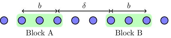
Figure 1: We compute the entanglement negativity ${\cal N}(b,\delta)$ for two blocks $A$ and $B$ consisting of $b$ sites each and separated by $\delta$ sites.

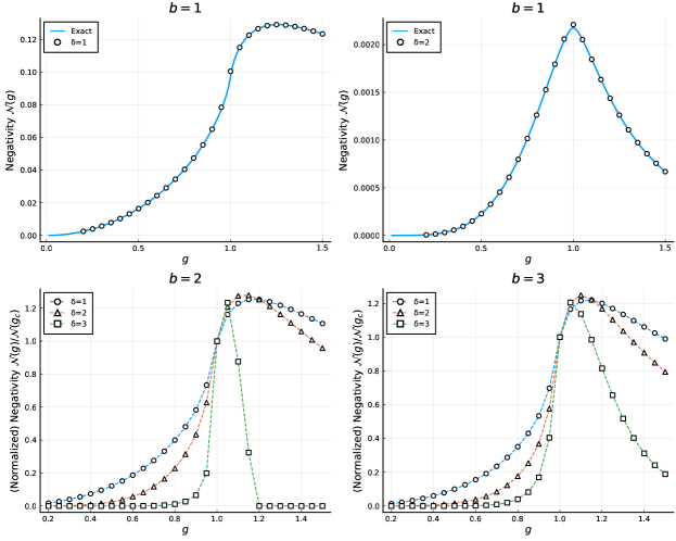
Figure 2: Entanglement negativity for lattice length $L=64$, blocksizes $b=1,2,3$ and seperations $\delta=1,2,3$ as function of the coupling $g$. The Top row shows results for $b=1$. The top-left plot shows nearest-neighbor negativity ($\delta=1$) and the top-right plot shows next-to-nearest neighbor negativity ($\delta=2$). (Negativity for $\delta=3$ is zero for $b=1$.) Since the negativities with $b=1$ can be computed exactly for the tfim (see Appendix E), we also show the exact results as thick solid lines. Bottom row: The left panel shows blocksize of $b=2$ while the right panel shows $b=3$ for various block separations $\delta=1,2,3$. Note that here we normalize the curves by $\mathcal{N}(g=1.0)$ to fit the various separations in the same figure. In all these cases (except $b=1,\delta=2$), we find that the maximum negativity is achieved slightly to the right of the critical point.

The lattice system of interest in our work is a one dimensional open chain of $L$ quantum spin-half particles interacting with the Hamiltonian which is the well known tfim [*[Seereview][andreferencestherein.]Stinchcombe_1973]. We label the sites of the spin chain as $i=1,2,...,L$ so that the Hamiltonian is given by

$$H=-\sum_{i=1}^{L-1}Z_{i}Z_{i+1}-g\sum_{i=1}^{L}X_{i},$$ (8)

where $X_{i},Y_{i},Z_{i}$ are the usual Pauli sigma matrices associated to the site $i$ and $g$ is the coupling to the transverse field. Note that the spin chain has open boundary conditions (obc). In the thermodynamic limit $(L\rightarrow\infty$) this model is known to have a second-order quantum phase transition at $g=1$ between an ordered phase ($g<1$) and a disordered phase ($g>1$). The local order parameter of the theory is the expectation value $\langle Z_{i}\rangle$ of the $z$-component of the quantum spin, and is related to the $\mathbb{Z}_{2}$ Ising symmetry of $H$ with the generator

$$Q=\prod_{i=1}^{L}X_{i}.$$ (9)

The ground state of the Hamiltonian Eq. 8 can be written as

$$\mathclose{\,\mathopen{|}\mathord{\Omega(g)}\mathclose{\rangle}}\ =\ \sum_{\sigma_{1},\dotsc,\sigma_{L}}\Psi(\sigma_{1},\sigma_{2},...,\sigma_{L})\ |\sigma_{1}\sigma_{2}\cdots\sigma_{L}\rangle$$ (10)

where $\sigma_{i}$ label some suitable eigenvalues of the local quantum spins. For example at extremely large $g$, the transverse-field term dominates and the (unique) ground state is just a product state of local eigenstates of $X_{i}$:

$$\mathclose{\,\mathopen{|}\mathord{\Omega(g\to\infty)}\mathclose{\rangle}}=\mathclose{\,\mathopen{|}\mathord{\rightarrow\cdots\rightarrow}\mathclose{\rangle}},$$ (11)

where $\mathclose{\,\mathopen{|}\mathord{\rightarrow}\mathclose{\rangle}}$ is the local eigenstate of $X$ with eigenvalue $1$. At the other extreme, when $g=0$, the ground state is doubly degenerate and the two basis states of this degenerate subspace can be chosen to be

$$\mathclose{\,\mathopen{|}\mathord{\Omega(0)^{+}}\mathclose{\rangle}} =\mathclose{\,\mathopen{|}\mathord{\uparrow\cdots\uparrow}\mathclose{\rangle}},$$ (12)

$$\mathclose{\,\mathopen{|}\mathord{\Omega(0)^{-}}\mathclose{\rangle}} =\mathclose{\,\mathopen{|}\mathord{\downarrow\cdots\downarrow}\mathclose{\rangle}}.$$ (13)

Note that $Q|{\Omega(0)^{+}}\rangle=\mathclose{\,\mathopen{|}\mathord{\Omega(0)^{-}}\mathclose{\rangle}}$. At some intermediate coupling the ground state is more complicated but can still be solved exactly for any value of the coupling $g$ [60]. Such a calculation uses the nonlocal Jordan-Wigner transformation to map the model into a free fermion model which can then be used to compute the ground state. For $g<1$, the ground state is doubly degenerate due to spontaneous symmetry breaking. Since we are interested in harvesting the entanglement of the ground state, we need to pick one of the two states in Eq. 13. To ensure that we always work with $|\Omega^{+}\rangle$ when $g<0$, we add a small pinning field at the boundary in our numerical calculations. Adding this pinning field then defines the ground state uniquely for all values of the coupling $g$.

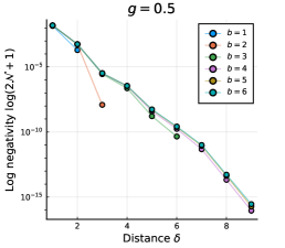
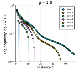
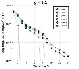
Figure 3: Sudden death of entanglement in the transverse field Ising model for various values of $g$. The various lines show the entanglement negativity as a function of the separation $\delta$ for different block sizes $b$. For small $b$, the negativity drops quickly to zero beyond some separation $\delta_{\text{max}}(b)$. As we increase the block size, $\delta_{\text{max}}$ becomes larger and we can separate the regions further while still having nonzero negativity. As we approach larger $b$, the decay is exponential with $\delta$, as expected from the literature. For $g<1$, the decay seems to be described roughly by an exponential function with a small wiggle. For $g\geq 1$ we notice that the wiggles turn into smoother oscillations.

Our goal is to compute the entanglement negativity of the ground state between two spatial regions $A$ and $B$ in the tfim as we discussed in the previous section. To define the negativity, we first note that the Hilbert space $\mathcal{H}$ of the full system $S$ factorizes into a tensor product of the local Hilbert spaces $\mathcal{H}_{i}$ at each lattice site $i\in S$, such that $\mathcal{H}=\otimes_{i\in S}\mathcal{H}_{i}$. We can identify two nonoverlapping set of sites, one of which belongs to $A$ (Alice) and the other to $B$ (Bob) and call the rest of the sites as $C$. The spins in each of the regions $A$ and $B$ will be assumed to be spatially connected but the two regions will be separated from each other. In Fig. 1 we show an illustration of such regions, where each region ($A$ or $B$) consists of $b$ sites and the two regions are separated by $\delta$ sites. We can express the ground state Eq. 10 as

$$\mathclose{\,\mathopen{|}\mathord{\Omega(g)}\mathclose{\rangle}}\ =\ \sum_{\sigma^{A},\sigma^{B},\sigma^{C}}\Psi(\sigma^{A},\sigma^{B},\sigma^{C})|\sigma^{A},\sigma^{B},\sigma^{C}\rangle$$ (14)

where $\sigma^{A},\sigma^{B},\sigma^{C}$ denote the collective spins in regions A,B,C, respectively. For example, $\sigma^{A}$ labels one of $2^{b}$ spin configurations within the region A and so on. The reduced density matrix of the subsystems $A\cup B$ can then be defined as

$$\rho^{\rm r}_{AB}=\operatorname{Tr}_{C}\rho\,.$$ (15)

where trace is over all spin degrees of freedom $\sigma^{C}$ in the region C that do not belong to either $A$ or $B$, and

$$\rho=|\Omega(g)\rangle\langle\Omega(g)|\,.$$ (16)

It is then possible to compute the entanglement negativity ${\cal N}(b,\delta;g)$ using Eq. 5 and understand how it depends on the block size, $b$ (assumed same for both), the separation between the blocks, $\delta$, and the coupling $g$ (See Fig. 1). Since our calculations are performed on a finite lattice with obc, we expect ${\cal N}(b,\delta;g)$ will also depend on the lattice size $L$ and where the two regions $A$ and $B$ are located with respect to the boundaries. To minimize such boundary contributions, we place $A$ and $B$ symmetrically on either side of the center of the quantum spin chain. Although the tfim can be solved exactly, it is difficult to compute ${\cal N}(b,\delta;g)$ analytically. For this reason, we use mps for our calculations. Some of the details of how our calculations are performed is explained in Appendix D.

In Fig. 2, we show the behaviour of the negativity ${\cal N}(b,\delta;g)$ as defined in Eq. 6 as a function of the coupling $g$ for a few values of seperation $\delta$ and block sizes $b$. For the block size $b=1$, we also compare against the exact results, explained briefly in Appendix E. At both extremes, $g=0$ and $g\to\infty$, the ground state is described by a product state and therefore the negativity vanishes as seen in our plots. It is well known that several entanglement measures display a qualitative change across a phase transition [61, 62]. The next-to-nearest-neighbor $b=1,\delta=2$ negativity ${\cal N}(1,2;g)$ shows a clear peak at the critical point $g=1$. However, the other negativities are not maximized exactly at the critical point, but for slightly larger $g$. From the point of view of this work, therefore, we would like the spin-chain to be close to criticality to extract the maximum amount of entanglement. For a condensed-matter system we can experimentally tune $g$ close to a transition, while for discussing continuum qft, we need to take the continuum limit which also arises close to the critical point. Unfortunately, the tensor network computations become difficult when correlation length diverges. Therefore, we choose a range of values around $g=g_{c}$ to perform our computations of the harvesting protocol.

The long distance physics of quantum many-body systems is described by quantum field theories. For critical systems, an analysis of negativity in conformal quantum field theories [65, 49, 48] shows that the logarithmic negativity $E_{N}$ decays exponentially: $E_{N}(b,\delta;g)\sim\exp(-c\,\delta/b)$ for some exponent $c$ and large enough $\delta$ and $b$ with $\delta/b$ finite. However, this negativity suddenly drops to zero as we increase the separation $\delta$, keeping $b$ and $g$ fixed, beyond some finite $\delta=\delta_{\text{max}}$ [*[Seereview][andreferencestherein]doi:10.1126/science.1167343]. We show our results for the exponential decay and this drop (called the sudden death of entanglement) in Fig. 3. For extracting negativities out of a finite spin system, this means that the separation is bounded by $\delta_{\text{max}}$. To take the continuum limit of our protocol, we would therefore have to increase both block sizes $b$ and separation $\delta$ while keeping $\delta/b$ fixed. Larger $b$ makes both the time-evolution and negativity computations harder. For this prototypical study, we set $b=1$ and hence are limited to $\delta=1$.

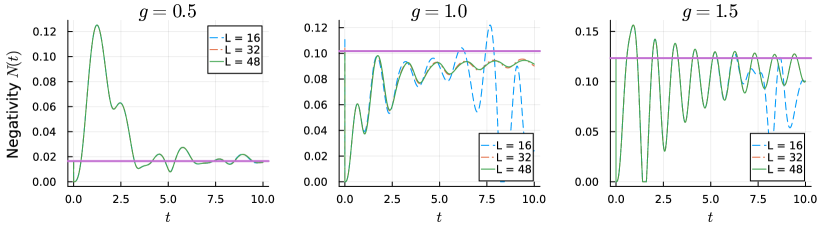
Figure 4: Here we show the time evolution of two-point negativity ${\cal N}_{1}(t)$ as a function of $t$ for various lattice sizes at different values of the coupling $g$, corresponding to $g=0.5$ (left,ordered), $g=1$ (center,critical) and $g=2$ (right,disordered) phases. The units of negativity are such that a bell-pair has negativity $\mathcal{N}=1$. The time is in units of inverse energy. We perform time evolution in steps of $\epsilon=0.01$ and perform $5000$ time steps. The solid horizontal line is the negativity ${\cal N}_{0}$ of the ground state of the tfim which is also the negativity obtained from $\rho^{R}_{0}$ after the first swap into the register $\alpha=0$. After this initial swap, we start measuring ${\cal N}_{1}(t)$ obtained from $\tilde{\rho}^{R}_{1}$ and so this negativity immediately drops to zero because at $t=0$ the spins were just swapped into the system. Then the negativity begins to grow as the state evolves according to the Hamiltonian of the the tfim. We note that there is a well-defined thermodynamic limit which is reached with $L=32$ in the range of times shown. Finite size effects cause fluctuations in the thermodynamic curve at large times, which are clearly visible in the $g=1.0$ and $g=1.5$ plots. In the thermodynamic limit, after a long time, the negativity ${\cal N}_{1}(t)$ goes back to its equilibrium value of ${\cal N}_{0}$ as expected. Fortunately, we can optimize the extracted negativity by using the first peak instead of the equilibrium value ${\cal N}_{0}$ which occurs at short times. For this we can work with smaller system sizes and in our work we use $L=16$ in all of our calculations.

IV Entanglement Harvesting Protocol

We now explain the protocol that we use to harvest entanglement from the spin chain of the tfim into two registers one of which is with Alice and the other with Bob. Each of these registers contains $N$ sets of $b$ quantum spins, the same size as $\sigma^{A}$ and $\sigma^{B}$, that are local to Alice or Bob. Let us label each set of $b$-spins as ${s^{A}}_{i}$ and $s^{B}_{i}$ where $i=0,1,2...,N-1$. The goal of our protocol is to create an entangled state of these two registers containing $2bN$ spins, by allowing them to temporarily interact with the spins $\sigma^{A}$ and $\sigma^{B}$ in the spin-chain of the tfim. These interactions can be viewed as discrete operations performed by Alice and Bob on the spin-chain and their registers. One particularly easy operation that Alice can perform is the unitary process $U^{A}_{\alpha}$ that ‘swaps’ the $b$ spins ${s^{A}}_{\alpha}$ that she has, with the $b$ spins $\sigma^{A}$ in the tfim. This process can be defined through the relation

$$U^{A}_{\alpha} |s^{A}_{1},..s^{A}_{\alpha},..s^{A}_{N}\rangle\otimes|s^{B}_{1},..s^{B}_{N}\rangle\otimes|\sigma^{A},\sigma^{B},\sigma^{C}\rangle$$

$$=|s^{A}_{1},..\sigma^{A},..s^{A}_{N}\alpha\rangle\otimes|s^{B}_{1},..s^{B}_{N}\rangle\otimes|s^{A},\sigma^{B},\sigma^{C}\rangle$$ (17)

Note that the Hilbert space basis now involves not only the spins of the tfim, but also those in the two registers, each with $bN$ spins. At the end of the swap process the wave function of the combined system $\psi(s^{A}_{1},..s^{A}_{\alpha},..;s^{B}_{1},..;\sigma^{A},\sigma^{B},\sigma^{C})$ changes to $\psi(s^{A}_{1},..\sigma^{A},..;s^{B}_{1},..;s^{A}_{\alpha},\sigma^{B},\sigma^{C})$ which means that if the wavefunction is written as a matrix in the product basis, the swap simply transposes the matrix in the relevant indices. Bob can perform a similar measurement through the process $U^{B}_{\alpha}$ which swaps $s^{B}_{\alpha}$ and $\sigma^{B}$. The two swaps commute: $U^{A}_{\alpha}U^{B}_{\alpha}=U^{B}_{\alpha}U^{A}_{\alpha}$.

In order to distill entanglement from the spin-chain into the registers, in our protocol Alice and Bob both begin with un-entangled spins in their registers and perform the swap $U^{A}_{0}U^{B}_{0}$ between their region of the spin-chain and the $\alpha=0$ set of $b$-spins of their registers. After the swap they allow the spin-chain to evolve according the Hamiltonian of tfim (i.e., without further interaction with the registers) for some time and again perform the swap, except this time they swap their respective regions of the spin chain with the $\alpha=1$ set of $b$-spins of their registers. This process continues and in general, at the $\alpha$th step, they perform the swap $U^{A}_{\alpha}U^{B}_{\alpha}$ between their region of the spin-chain and the $\alpha$th set of $b$-spins of their registers. The entanglement properties that are distilled from the spin-chain can be studied using the reduced density matrix of the registers $\rho^{R}_{\alpha}$ after swapping the $\alpha$th set of $b$-spins in the registers. Note that $\rho^{R}_{\alpha}$ is a $2^{2b(\alpha+1)}\times 2^{2b(\alpha+1)}$ matrix. As we explain below, it is useful to discard the $\alpha=0$ spins of the registers (trace over them) and define $\tilde{\rho}^{R}_{\alpha}$ which is a $2^{2b\alpha}\times 2^{2b\alpha}$ matrix.

IV.1 Results: Single step

As mentioned earler, the amount of entanglement that can be distilled out of the registers is bounded by the logarithmic negativity of $\tilde{\rho}^{R}_{\alpha}$, but we can build up this negativity by making $\alpha$ large (i.e., repeat the swap process several times). However, the timings when the swaps are performed can also play a role. In order to understand how to efficiently build up the negativity in the registers, we now study how it builds up in the spin-chain as it evolves following a swap. To this end, we study the simple case of $b=1$ and $\delta=1$. We begin with the spin-chain in the ground state of the tfim and perform the first swap ($U^{A}_{0}U^{B}_{0}$) at time $t=0$. Let us define ${\cal N}_{0}$, as the negativity obtained from $\rho^{R}_{0}$ after this swap. This is the negativity between the swapped spins in the ground state of the tfim. After this initial swap let us allow the spin-chain to evolve according to Eq. 8 for a time $t$ before performing the second swap ($U^{A}_{1}U^{B}_{1}$). After this second swap we can compute the density matrix $\tilde{\rho}^{R}_{1}(t)$, and the associated negativity ${\cal N}_{1}(t)$ as discussed in Section II. In Fig. 4, we plot the time evolution of ${\cal N}_{1}(t)$ in the three phases as a function of the system size $L$. Note that ${\cal N}_{1}(t)$ vanishes at $t=0$ since the spins swapped into the spin chain have not yet had the time to evolve, but then begins to build up. Further, it is described by a well defined function of $t$ in the thermodynamic limit, which starts at the origin as expected and approaches ${\cal N}_{0}$ in the limit $t\rightarrow\infty$. At intermediate times it oscillates and reaches a maximum at some $t=t_{\rm min}(g)$, where ${\cal N}_{1}(t_{\rm min})>{\cal N}_{0}$ in both the ordered and disordered phases.

$g=0.5,L=16$
1.000	0.708	0.710	0.713	0.715
	1.000	0.999	0.997	0.994
		1.000	0.999	0.997
			1.000	0.999
				1.000

$g=0.75,L=16$
1.000	0.710	0.720	0.727	0.728
	1.000	0.997	0.990	0.981
		1.000	0.997	0.991
			1.000	0.998
				1.000

$g=1.25,L=16$
1.000	0.700	0.760	0.768	0.760
	1.000	0.988	0.984	0.988
		1.000	1.000	1.000
			1.000	1.000
				1.000

$g=1.5,L=16$
1.000	0.700	0.766	0.751	0.741
	1.000	0.990	0.994	0.996
		1.000	0.999	0.998
			1.000	1.000
				1.000

Table 1: Fidelity $F(\bar{\rho}_{i},\bar{\rho}_{j})$ between different $\bar{\rho}_{i}$’s where $i=0,1,2,3,4$. Each $\bar{\rho}_{i}$ is a $4\times 4$ matrix of the $i$th spin-pair obtained by tracing $\rho^{R}_{\alpha=4}$ over the remaining spin-pairs.

$g=0.50,\ L=16$
$\alpha$	$f_{R,S}$	$f_{R,P}$	$f_{S,SP}$	$\tilde{f}_{R,S}$	$\tilde{f}_{R,P}$	$\tilde{f}_{S,SP}$
0	1.000	1.000	1.000	-	-	-
1	0.923	0.991	0.969	1.000	1.000	1.000
2	0.922	0.989	0.974	1.000	0.996	0.996
3	0.929	0.988	0.978	0.999	0.994	0.996
4	0.935	0.989	0.982	0.998	0.994	0.996

$g=0.75,\ L=16$
$\alpha$	$f_{R,S}$	$f_{R,P}$	$f_{S,SP}$	$\tilde{f}_{R,S}$	$\tilde{f}_{R,P}$	$\tilde{f}_{S,SP}$
0	1.000	1.000	1.000	-	-	-
1	0.925	0.986	0.960	1.000	1.000	1.000
2	0.923	0.983	0.970	0.999	0.994	0.995
3	0.928	0.983	0.978	0.996	0.992	0.996
4	0.933	0.985	0.984	0.993	0.992	0.997

$g=1.25,\ L=16$
$\alpha$	$f_{R,S}$	$f_{R,P}$	$f_{S,SP}$	$\tilde{f}_{R,S}$	$\tilde{f}_{R,P}$	$\tilde{f}_{S,SP}$
0	1.000	1.000	1.000	-	-	-
1	0.926	0.983	0.949	1.000	1.000	1.000
2	0.920	0.979	0.971	0.991	0.991	0.996
3	0.922	0.978	0.983	0.986	0.988	0.997
4	0.926	0.977	0.988	0.983	0.985	0.997

$g=1.50,\ L=16$
$\alpha$	$f_{R,S}$	$f_{R,P}$	$f_{S,SP}$	$\tilde{f}_{R,S}$	$\tilde{f}_{R,P}$	$\tilde{f}_{S,SP}$
0	1.000	1.000	1.000	-	-	-
1	0.924	0.985	0.950	1.000	1.000	1.000
2	0.916	0.977	0.973	0.987	0.987	0.996
3	0.915	0.973	0.983	0.982	0.982	0.995
4	0.917	0.970	0.988	0.978	0.977	0.996

Table 2: Comparison of various density matrices discussed in the text using Fidelity $f_{X,Y}=f(\rho^{X}_{\alpha},\rho^{Y}_{\alpha})$ and $\tilde{f}_{X,Y}=f(\tilde{\rho}^{X}_{\alpha},\tilde{\rho}^{Y}_{\alpha})$, defined using the relation Eq. 23.

$g=0.5,\ L=16$
$\alpha$	$E_{1}$	$E_{2}$	$E_{3}$	$\tilde{E}_{2}$	$\tilde{E}_{3}$
0	0.05	0.05	0.05	-	-
1	0.03	0.07	0.00	0.03	0.03
2	0.03	0.07	0.00	0.04	0.03
3	0.03	0.07	0.00	0.04	0.03
4	0.05	0.07	0.01	0.05	0.03

$g=0.75,\ L=16$
$\alpha$	$E_{1}$	$E_{2}$	$E_{3}$	$\tilde{E}_{2}$	$\tilde{E}_{3}$
0	0.12	0.12	0.12	-	-
1	0.08	0.14	0.00	0.08	0.08
2	0.08	0.14	-0.00	0.09	0.07
3	0.11	0.14	0.00	0.11	0.08
4	0.15	0.14	0.01	0.12	0.09

$g=1.25,\ L=16$
$\alpha$	$E_{1}$	$E_{2}$	$E_{3}$	$\tilde{E}_{2}$	$\tilde{E}_{3}$
0	0.33	0.33	0.33	-	-
1	0.21	0.29	0.00	0.21	0.21
2	0.27	0.30	-0.00	0.26	0.23
3	0.29	0.31	0.02	0.28	0.24
4	0.27	0.31	0.06	0.28	0.25

$g=1.5,\ L=16$
$\alpha$	$E_{1}$	$E_{2}$	$E_{3}$	$\tilde{E}_{2}$	$\tilde{E}_{3}$
0	0.32	0.32	0.32	-	-
1	0.28	0.32	-0.00	0.28	0.28
2	0.34	0.34	0.01	0.33	0.30
3	0.32	0.35	0.07	0.34	0.31
4	0.31	0.35	0.11	0.35	0.31

Table 3: The log-negativity defined through $E_{1}=E_{N}(\bar{\rho}^{R}_{\alpha})$, $E_{2}=E_{N}(\rho^{R}_{\alpha})/(\alpha+1)$, $E_{3}=E_{N}(\bar{\rho}^{S}_{\alpha})$, $\tilde{E}_{2}=E_{N}(\tilde{\rho}^{R}_{\alpha})/\alpha$, $\tilde{E}_{3}=E_{N}(\bar{\tilde{\rho}}^{S}_{\alpha})$ where $E_{N}(\rho)$ was defined in Eq. 6. Note that $\tilde{E}_{1}\equiv E_{N}(\bar{\tilde{\rho}}^{R}_{\alpha})=E_{1}$ by definition.

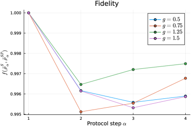
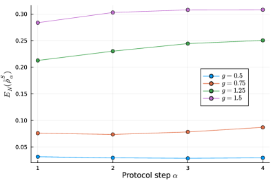
Figure 5: The plot the fidelity per spin-pair $f(\tilde{\rho}^{S}_{\alpha},\tilde{\rho}^{SP}_{\alpha})$ (left), and the negativity $E_{N}(\bar{\tilde{\rho}}^{S}_{\alpha})$ as a function of the number of spin-pairs extracted. Left panel: Data is given in Table 2 under $\tilde{f}_{S,SP}$. This figure shows that the symmetrized state is close to a product state. Right panel: $\tilde{E}_{3}$ in Table 3.

IV.2 Results: Multiple steps

Having investigated the rise of entanglement in the register after the first swap, we now construct a protocol to build up entanglement in the registers as a function of $\alpha$. Since ${\cal N}_{1}(t)$, defined in the previous section, is maximized when $t=t_{\rm min}(g)$, we choose to perform the $\alpha$th swap at the times $t_{\alpha}=\alpha t_{\rm min}(g)$ for each value of $g$. We can then compute both the density matrices $\rho^{R}_{\alpha}$ and $\tilde{\rho}^{R}_{\alpha}$ to study how the entanglement depends on $\alpha$.

Any protocol to extract entanglement from the registers will need access to the density matrix $\rho^{R}_{\alpha}$. Unfortunately, there is no practical way to measure the density matrix of a single quantum system without destroying the state. Measurement of density matrices are, however, possible with access to an infinite number of independent identical systems. In fact to use the distillation protocol defined in Eq. 7, we already assume the quantum state of the register to be in a direct product of independent and identical quantum systems, each of size $b$ spin-pairs. This means we would ideally like to have

$$\rho^{R}_{\alpha}=\ \underbrace{\bar{\rho}\otimes\bar{\rho}\otimes...\otimes\bar{\rho}}_{(\alpha+1)\text{ copies}},$$ (18)

where $\bar{\rho}$ is a $2b\times 2b$ matrix whose properties can be used to practically to extract entanglement especially when $\alpha$ is large. This form implies two results: first, all the $\alpha+1$ $b$ spin pairs are in an identical state, and second, they are independent so that $\rho_{\alpha}^{R}$ is a direct product. To check the first, we compute $\bar{\rho}^{R}_{i},i=0,1,2,..,\alpha$ as the $2^{2b}\times 2^{2b}$ matrix of the $i$th $b$ spin-pair obtained by tracing $\rho^{R}_{\alpha}$ over the remaining spin-pairs and check how similar $\bar{\rho}^{R}_{i},i=0,1,2,..,\alpha$ are to each other. One way to check this is to compute the fidelity $F(\bar{\rho}^{R}_{i},\bar{\rho}^{R}_{j})$ between these matrices where the Fidelity is defined through the expression

$$F(\rho_{i},\rho_{j})\ =\ \Big{(}\mathrm{tr}\Big{[}\sqrt{\sqrt{\rho_{i}}\rho_{j}\sqrt{\rho}_{i}}\Big{]}\Big{)}^{2}.$$ (19)

If the two density matrices are similar, then this quantity will be close to one. Second we need to check if $\rho^{R}_{\alpha}$ is indeed the same as density matrix constructed as

$$\rho^{P}_{\alpha}=\ \bar{\rho}^{R}_{0}\otimes\bar{\rho}^{R}_{1}...\otimes\bar{\rho}^{R}_{\alpha}.$$ (20)

We can again do this by computing the Fidelity $F(\rho^{R}_{\alpha},\rho^{P}_{\alpha})$ and making sure that it is close to one.

Finally, if we do not distinguish between the $\alpha+1$ $b$ spin pairs in our distillation protocol, we can choose to consider a symmetrized density matrix $\rho^{S}_{\alpha}$ as discussed in Appendix B. Due to the quantum de Finniti theorem [69, 70], this symmetrized density matrix is known to take the form

$$\rho^{S}_{\alpha}\ =\ \underbrace{\bar{\rho}\otimes\bar{\rho}\otimes...\otimes\bar{\rho}}_{(\alpha+1)\text{ copies}},$$ (21)

in the limit $\alpha\rightarrow\infty$. Here $\bar{\rho}$ is a $2^{2b}\times 2^{2b}$ density matrix of $b$ spin-pairs, while $\rho^{R}_{\alpha}$ was a $2^{2b(\alpha+1)}\times 2^{2b(\alpha+1)}$ matrix. When $\alpha$ is not infinite we do not expect $\rho^{S}_{\alpha}$ to be of the form Eq. 21 but we can again ask how close to it do we get. As in the case of $\rho^{R}_{\alpha}$, we can again compute $\bar{\rho}^{S}_{i},i=0,1,...,\alpha$. But since $\rho^{S}_{\alpha}$ is symmetrized we will find $\bar{\rho}^{S}_{0}=\bar{\rho}^{S}_{1}=...=\bar{\rho}^{S}_{\alpha}$. We can also construct

$$\rho^{SP}_{\alpha}=\ \underbrace{\bar{\rho}^{S}_{\alpha}\otimes\bar{\rho}^{S}_{\alpha}...\otimes\bar{\rho}^{S}_{\alpha}}_{(\alpha+1)\text{ copies}}$$ (22)

and compare it with $\rho^{S}_{\alpha}$ for various $\alpha$’s. Note that we defined $\rho^{P}_{\alpha}$, $\rho^{S}_{\alpha}$, $\rho^{SP}_{\alpha}$ starting from $\rho^{R}_{\alpha}$. We can similarly define $\tilde{\rho}^{P}_{\alpha}$, $\tilde{\rho}^{S}_{\alpha}$, $\tilde{\rho}^{SP}_{\alpha}$ starting from $\tilde{\rho}^{R}_{\alpha},\alpha=1,2,..$ which is obtained from $\rho^{R}_{\alpha}$ by tracing over the zeroth $b$ spin-pair (i.e., $\tilde{\rho}^{R}_{0}=1$). Note that $\tilde{\rho}^{R}_{\alpha}$ will be a $2^{2b\alpha}\times 2^{2b\alpha}$ matrix. We will see below that $\tilde{\rho}^{R}_{\alpha}$ and $\tilde{\rho}^{S}_{\alpha}$ are closer to the form described by Eq. 18 and Eq. 21 with $\alpha$-copies than $\rho^{R}_{\alpha}$ and $\rho^{S}_{\alpha}$.

In our work we choose $b=1$, $\delta=1$, $L=16$ and assume we have up to $N=5$ spin-pairs in the register. Thus we can compute the sequence of density matrices $\rho^{R}_{\alpha},\alpha=0,1,2,3,4$ of sizes $4^{(\alpha+1)}\times 4^{(\alpha+1)}$. For $\alpha=4$ we can compute $\bar{\rho}^{R}_{i},i=0,1,2,3,4$ which are $4\times 4$ matrices. In Table 1 we show the results for $F(\bar{\rho}_{i},\bar{\rho}_{j})$ at $g=0.5,1.0$ and $1.5$. Based on these results we note that $\bar{\rho}^{R}_{0}$, obtained after the first swap, is quite different from the remaining. The other four density matrices are very similar. This suggests that it may be better to trace over $\alpha=0$ spin-pairs and focus on $\tilde{\rho}^{R}_{\alpha}$.

$g=0.5,\ L=16$
$i$	$F_{m}$	$\theta$	$\phi$	$\beta$
0	$0.52$	$0.79$	$0.00$	$1.57$
1	$0.51$	$0.72$	$0.34$	$-0.60$
2	$0.51$	$0.73$	$0.32$	$-0.43$
3	$0.51$	$0.74$	$0.30$	$-0.19$
4	$0.52$	$0.75$	$0.28$	$0.00$
5	$0.52$	$0.75$	$0.27$	$0.13$
6	$0.53$	$0.75$	$0.27$	$0.20$

$g=0.75,\ L=16$
$i$	$F_{m}$	$\theta$	$\phi$	$\beta$
0	$0.54$	$0.79$	$0.00$	$1.57$
1	$0.52$	$0.66$	$0.46$	$-0.44$
2	$0.53$	$0.69$	$0.42$	$-0.14$
3	$0.54$	$0.71$	$0.38$	$0.11$
4	$0.55$	$0.71$	$0.37$	$0.24$
5	$0.56$	$0.71$	$0.36$	$0.28$

$g=1.25,\ L=16$
$i$	$F_{m}$	$\theta$	$\phi$	$\beta$
0	$0.26$	$0.00$	$0.79$	$0.01$
1	$0.58$	$0.60$	$0.54$	$0.07$
2	$0.60$	$0.65$	$0.48$	$0.36$
3	$0.61$	$0.65$	$0.47$	$0.39$
4	$0.60$	$0.65$	$0.48$	$0.36$

$g=1.5,\ L=16$
$i$	$F_{m}$	$\theta$	$\phi$	$\beta$
0	$0.62$	$0.79$	$0.00$	$-1.57$
1	$0.61$	$0.59$	$0.55$	$0.28$
2	$0.63$	$0.64$	$0.49$	$0.49$
3	$0.62$	$0.63$	$0.50$	$0.44$
4	$0.62$	$0.63$	$0.51$	$0.41$

Table 4: The maximum singlet fraction $F_{m}$ of $i$-th extracted spin pair computed using $\bar{\rho}^{R}_{i}$. In each case we also give the angles to the closest maximally entangled state, parameterized through Eq. 60.

$g=0.5$, $L=16$
	keeping zeroth spin				dropping zeroth spin
$\alpha$	$F_{m}$	$\theta$	$\phi$	$\beta$	$F_{m}$	$\theta$	$\phi$	$\beta$
0	$0.52$	$0.79$	$0.00$	$1.57$	-	-	-	-
1	$0.48$	$0.77$	$0.19$	$-1.43$	$0.51$	$0.72$	$0.34$	$-0.60$
2	$0.48$	$0.75$	$0.26$	$-0.81$	$0.51$	$0.72$	$0.33$	$-0.52$
3	$0.49$	$0.75$	$0.26$	$-0.43$	$0.51$	$0.73$	$0.32$	$-0.41$
4	$0.49$	$0.75$	$0.25$	$-0.24$	$0.51$	$0.73$	$0.31$	$-0.30$

$g=0.75$, $L=16$
	keeping zeroth spin				dropping zeroth spin
$\alpha$	$F_{m}$	$\theta$	$\phi$	$\beta$	$F_{m}$	$\theta$	$\phi$	$\beta$
0	$0.54$	$0.79$	$0.00$	$1.57$	-	-	-	-
1	$0.47$	$0.75$	$0.26$	$-1.51$	$0.52$	$0.66$	$0.46$	$-0.44$
2	$0.46$	$0.70$	$0.39$	$-0.62$	$0.52$	$0.67$	$0.44$	$-0.29$
3	$0.48$	$0.72$	$0.34$	$-0.05$	$0.53$	$0.68$	$0.42$	$-0.15$
4	$0.49$	$0.73$	$0.33$	$0.09$	$0.53$	$0.69$	$0.41$	$-0.04$

$g=1.25$, $L=16$
	keeping zeroth spin				dropping zeroth spin
$\alpha$	$F_{m}$	$\theta$	$\phi$	$\beta$	$F_{m}$	$\theta$	$\phi$	$\beta$
0	$0.26$	$0.00$	$0.79$	$0.01$	-	-	-	-
1	$0.43$	$0.75$	$0.26$	$-1.72$	$0.58$	$0.60$	$0.54$	$0.07$
2	$0.45$	$0.64$	$0.50$	$0.49$	$0.59$	$0.62$	$0.52$	$0.22$
3	$0.49$	$0.64$	$0.49$	$0.44$	$0.59$	$0.63$	$0.50$	$0.28$
4	$0.51$	$0.64$	$0.49$	$0.41$	$0.59$	$0.64$	$0.50$	$0.30$

$g=1.5$, $L=16$
	keeping zeroth spin				dropping zeroth spin
$\alpha$	$F_{m}$	$\theta$	$\phi$	$\beta$	$F_{m}$	$\theta$	$\phi$	$\beta$
0	$0.62$	$0.79$	$0.00$	$1.57$	-	-	-	-
1	$0.43$	$0.66$	$0.46$	$0.96$	$0.61$	$0.59$	$0.55$	$0.28$
2	$0.49$	$0.61$	$0.53$	$0.65$	$0.62$	$0.61$	$0.52$	$0.39$
3	$0.52$	$0.61$	$0.53$	$0.56$	$0.62$	$0.62$	$0.52$	$0.41$
4	$0.54$	$0.61$	$0.53$	$0.52$	$0.62$	$0.62$	$0.52$	$0.41$

Table 5: The maximum singlet fraction $F_{m}$ computed using $\bar{\rho}^{S}_{\alpha}$ and the closest maximally entangled state, parameterized as in Eq. 60. Similarly $\tilde{F}_{m}$ refers to the maximal singlet fraction computed using $\bar{\tilde{\rho}}^{S}_{\alpha}$ where the zeroth spin-pair was ignored. Note that all unentangled states have $f\leq 0.5$ [71], the actual entanglement negativities are presented in Table 3.

In Table 2 we compare the matrices $\rho^{R}_{\alpha}$, $\rho^{P}_{\alpha}$, $\rho^{S}_{\alpha}$ and $\rho^{SP}_{\alpha}$. Since these are density matrices involving different number of spin-pairs, instead of using the fidelity defined in Eq. 19, we define the fidelity per spin-pair using the $k$th root of the Fidelity defined as

$$f(\rho,\rho^{\prime})=(F(\rho,\rho^{\prime}))^{1/k}$$ (23)

where $k$ labels the number of spin-pairs that the density matrices $\rho$ and $\rho^{\prime}$ describe. We notice again that dropping the zeroth spin-pair is very helpful and $\tilde{\rho}^{R}_{\alpha}$ is well described by a product state and symmetrization helps improve things. In Fig. 5 we plot the fidelity $f(\tilde{\rho}^{S}_{\alpha},\tilde{\rho}^{SP}_{\alpha})$ and the logarithmic negativity $E_{N}(\bar{\tilde{\rho}}^{S}_{\alpha})$ as a function of $\alpha$.

As described in Appendix B, most distillation protocols only have access to the symmetrized part of the density matrix of spin-pairs extracted at different times. While the different spin-pairs can be entangled to roughly the same extent, they can be aligned in different directions. In such situations the symmetrized density matrix is likely to be less entangled and can even be unentangled. This can be seen in our results in Table 3, where we compute the logarithmic negativity extracted from $\bar{\rho}^{R}_{\alpha}$, $\rho^{R}_{\alpha}$ and $\bar{\rho}^{S}_{\alpha}$. Note that while $E_{N}(\bar{\rho}^{R}_{1})$ and $E_{N}(\rho^{R}_{1})/2$ are non-zero, $E_{N}(\bar{\rho}^{S}_{1})$ vanishes. This means that though the zeroth spin-pair and the first spin-pair are both entangled, symmetrization kills this entanglement, suggesting that both spin-pairs are entangled but aligned differently. We discuss this issue of alignment more clearly in Appendix F by defining the maximal singlet fraction $F_{m}(\rho)$ for a given density matrix $\rho$ and explain how we can use it to construct the density matrix $\rho^{A}$ that is aligned properly. So instead of symmetrizing $\rho^{R}_{\alpha}$ it may actually be necessary to symmetrize $\rho^{A}_{\alpha}$ while constructing $\rho^{S}_{\alpha}$. Let us explore if this is necessary in our case.

In order to study how the various extracted spin-pairs are aligned, in Table 4 we compute the singlet fraction $F_{m}$ of each extracted spin-pair using $\bar{\rho}^{R}_{i},i=0,1,2,3,4$ obtained from $\rho^{R}_{\alpha=4}$. We also compute the nearest corresponding maximal Bell-state using three angles $\theta$, $\phi$ and $\beta$ as defined in Eq. 60. Note that although $F_{m}$ is roughly the same for all the five spin-pairs, the closest maximally entangled state for the zeroth pair is aligned very differently than the remaining pairs which are more closely aligned. This is the reason that in Table 3, while $E_{N}(\bar{\rho}^{R}_{0})$ and $E_{N}(\bar{\rho}^{R}_{1})$ are non-zero showing these spin-pairs are entangled, $E_{N}(\bar{\rho}^{S}_{1})$ vanished since symmetrization killed the negativity. This is again consistent with our previous observation that it is best to discard the zeroth spin-pair. The importance of dropping the zeroth spin-pair is also visible in Table 5, where we compute the maximal singlet fraction $F_{m}$ for each spin pair obtained from the symmetrized density matrix, $\bar{\rho}^{S}_{\alpha}$ and compare it with $\bar{\tilde{\rho}}^{S}_{\alpha}$ where the zeroth spin pair is dropped. When we keep the zeroth spin-pair during the symmetrization procedure, $F_{m}$ initially drops and then slowly begins to build back as more and more aligned spin-pairs are added to the register. On the other hand if we ignore the zeroth spin-pair, $F_{m}$ changes only slightly as the spin-pairs accumulate in the register. This suggests that we do not need to explicitly align the spin pairs in our protocol if we ignore the zeroth spin pair.

V Conclusions

We have studied the dynamics of entanglement in the ground state of the one-dimensional tfim, in particular, how the entanglement recovers after it is externally set to zero. We find that the entanglement rebounds and oscillates, asymptotically reaching its ground-state value at long times. This allows us to repeatedly extract this entanglement into a register—and the extracted entanglement can be optimized by choosing the interval between extractions to be equal to the time of the first rebound peak. Finally, we find that the pairs extracted near this peak of each rebound are almost aligned, and can be used in a standard protocol to distill Bell pairs.

In this first study, we could only look at single spin-pairs separated by a distance of one lattice spacing in a one dimensional spin chain. Further work is necessary to see how the results generalize to the interesting case of blocks of spins-pairs and separations that are a non-zero fraction of the correlation length. We can then connect the results with entanglement extraction from continuum quantum field theory that emerges as one approaches the critical point at $g=1$. Numerically, this requires both large block sizes $b$ and separations $\delta$ with $\delta/b$ kept fixed.

An important feature of this approach to entanglement harvesting protocol is its feasibility on near-term analog and digital quantum devices. For example, Ising-like interactions can be natively generated on cold-atom simulators based on Rydberg atoms [72], and local entangling operations between qubits have been demonstrated [73]. It would be interesting to explore whether this simple protocol can be implemented on quantum hardware to generate Bell pairs from the vacuum of a spin chain.

Appendix A Density Matrices

In this section we review some well known ideas about density matrices, to help a reader who may not be familiar with them. First we note that it is always possible to reformulate everything in quantum mechanics using the concept of a density matrix $\rho$ of a quantum state. For example, given a normalized state $|\psi\rangle$ in the Hilbert space of a quantum system, we can construct the density matrix $\rho\equiv|\psi\rangle\langle\psi|$. It is then easy to see that the operator $|\psi\rangle\to\hat{O}|\psi\rangle$ can be implemented directly on the density matrix as $\rho\to\hat{O}\rho\hat{O}^{\dagger}$. Moreover, the probability that observable $\hat{O}$ takes the value $o$ in a projective measurement is given by

$$\sum_{\psi^{o}_{i}}|\langle\psi|\psi^{o}_{i}\rangle|^{2}\equiv\operatorname{Tr}\rho P^{o}\,,$$ (24)

where $\{|\psi^{o}_{i}\rangle\}$ is a basis for the eigen-subspace of $\hat{O}$ with eigenvalue $o$ and $P^{o}\equiv\sum_{\psi^{o}_{i}}|\psi^{o}_{i}\rangle\langle\psi^{o}_{i}|$ is the projector into this eigen-subspace. In addition, in this case, the posterior state conditioned on the observation is given by $\rho P^{o}/\operatorname{Tr}\rho P^{o}$. In other words, all properties of a pure state in the Hilbert space of a quantum system can be studied using the density matrix.

When we are dealing with subsystems of quantum systems, it is more economical to introduce the concept of a density matrix, since pure states would require us to consider the entire quantum system. If we are only interested in the subsystem, which could be much smaller than the entire quantum system, then we can treat the subsystem as a quantum system in a mixed state described by a density matrix. We can define the density matrix of the entire system as the full density matrix, while the density matrix of the subsystem as the reduced density matrix obtained as the partial trace of the full density matrix over the Hilbert space complementary to the subsystem.

The equivalence of the two pictures—dealing with the density matrix of the entire subsystem or the reduceded density matrix of only the subsystem of interest—is most easily explained by the notion of an effective density matrix, which also generalizes the concept of the reduced density matrix. Here we explain this idea, as motivated in Casini et al. [77, Section 3.2], but generalized to be more appropriate for our work. The idea of an effective density matrix arises from the fact that a subsystem is associated with a set of observables that act only on it, and thus with an algebra of a subset of operators $\{\hat{O}\}$ of interest, all of which are invariant under an unitary group of transformations $\{U\}$ of the complementary subsystems:

$$U\hat{O}U^{\dagger}=\hat{O}\qquad$$ (25)

for all $U$ and $\hat{O}$. Then, for any density matrix $\rho$,

$$\operatorname{Tr}\hat{O}\rho =\Big{\langle}\operatorname{Tr}\big{(}U\ \hat{O}\ U^{\dagger}\rho\big{)}\Big{\rangle}_{U}\ =\ \operatorname{Tr}\hat{O}\rho^{e}\,,$$ (26)

where $\langle\ \dots\ \rangle_{U}$ represents the mean over all unitary transformations in the group and

$$\rho^{e}=\Big{\langle}U^{\dagger}\rho\ U\Big{\rangle}_{U}\,.$$ (27)

is the effective density matrix given as the ‘singlet’ projection of $\rho$ under the unitary group. Stated in words, if we only have access to operators that are invariant under the unitary group, then Eq. 26 means that we have access only to this projection of $\rho$ and so we can replace it by $\rho^{e}$ in all calculations. Note that we can choose the mean in Eq. (27) to be over a group invariant measure, so that evolution of $\rho$ by any unitary $\hat{V}\in\{U\}$, such that $\rho\to V\ \rho V^{\dagger}$, will leave $\rho^{e}$ unchanged since

$$\langle U^{\dagger}\hat{V}\rho\hat{V}^{\dagger}U\rangle_{U}\ =\ \rho_{e}.$$ (28)

Because of this, projection of $\rho$ to $\rho^{e}$ commutes with any evolution of the form $\prod_{i}\hat{U}_{i}$, where each $\hat{U}_{i}$ is either an element of $\{U\}$, or commutes with all of them. In our example, this means that $\rho^{e}$ is not changed by evolutions that act independently on the subsystem of interest and its complement.

We can connect the concept of an effective density matrix to the standard idea of the reduced density matrix by considering the Hilbert space of the full system $S$ as a direct product of two subsystems $A$ and $C$. Let us write the operators and density matrices in a direct product basis. Thus $\rho\equiv\sum_{aa^{\prime},cc^{\prime}}\rho_{ac;a^{\prime}c^{\prime}}(|a\rangle\otimes|c\rangle)(\langle a^{\prime}|\otimes\rangle c^{\prime}|)$. Then the standard definition of the reduced density matrix for the first subsystem given by

$$\rho^{r}_{A}\ =\ \sum_{aa^{\prime},c}\rho_{ac;a^{\prime}c}|a\rangle\langle a^{\prime}|$$ (29)

On the other hand we can define the first subsystem as associated with observables of the form $(\hat{O}\otimes\hat{I})$, all of which are invariant under the unitary group $(I\otimes U)$. It is then easy to see that

$$\Big{\langle}\ (I\otimes U)^{\dagger}\ (|a\rangle\otimes|c\rangle) (\langle a^{\prime}|\otimes\rangle c^{\prime}|)\ (I\otimes U)\ \Big{\rangle}_{U}$$

$$=\ \delta_{cc^{\prime}}\ (|a\rangle\otimes|c\rangle)(\langle a^{\prime}|\otimes\rangle c^{\prime}|)$$ (30)

From this we obtain

$$\rho^{e}\ =\ \langle(I\otimes U)^{\dagger}\ \rho\ (I\otimes U)\rangle_{U}\ =\ \rho^{r}_{A}\otimes I.$$ (31)

The condition for the reduction to commute with the evolution, then, means that we need the evolution to be a product of evolutions acting on the two systems independently, i.e., there is no interaction between the two subsystems.

Appendix B Permutation Symmetric Density Matrix

Consider the Hilbert space of the register of spins that Alice and Bob have. Let us label the basis states of this space as $\bigotimes_{i=0,\ldots,N-1}|s_{i}\rangle$, where $s_{i}$ stands for $2b$ spins. Now, we study the permutation symmetric version of an $n$-subsystem operator on this space. For this we consider operators $O_{n}$ that act nontrivially only on the first $n$ subsystems. Let us define an operator

$$O^{S,m}_{n}\equiv\Big{\langle}{\cal P}_{m}O_{n}{\cal P}^{\dagger}_{m}\Big{\rangle}_{{\cal P}_{m}}$$ (32)

where ${\cal P}_{m}$ is an element of the group of permutation operators that permute the first $m\geq n$, $2b$ spins. Using the arguments of Appendix A we can see that the operators $O^{S,m}_{n}$ can only access to the reduced density matrix $\rho^{r}_{m}$ where all subsystems beyond the $m^{\rm th}$ have been traced over. Furthermore, because of the permutation symmetry, not even the whole reduced density matrix is accessible, but only the effective density matrix

$$\rho^{S}_{m}=\Big{\langle}{\cal P}_{m}^{\dagger}\rho_{m}{\cal P}_{m}\Big{\rangle}_{{\cal P}_{m}}.$$ (33)

Given any set of operators $\{O_{n}\}$, the same density matrices $\rho^{S}_{m}$ suffice to give not only the mean values of $O_{n}$ over the permutation group, but also other permutation invariant functions such as their variances and all higher cumulants over the permutation group, and hence the entire joint distribution of any commuting subset of them.

The matrices $\rho^{S}_{m}$ for $n\leq m\leq N$ form a sequence of permutation symmetric density matrices such that $\rho^{S}_{m}$ is the partial trace of $\rho^{S}_{m+1}$ by construction. When $N$ is strictly infinite, by the quantum de Finetti theorem [69, 70], we can write $\rho^{S}_{m}$ as an average over direct product of single system subsystems, i.e.,

$$\rho^{S}_{m}\ =\ \int d\rho\ p(\rho)\ \bigotimes_{m}\rho$$ (34)

for all $m$, where $p(\rho)$ is some probability density of density matrices $\rho$ of one subsystem, and $\bigotimes_{m}\rho$ stands for the direct product of $m$ copies of $\rho$. As a final step, note that if the variance of every $O_{n}$ over the permutation group of size $m$ vanishes as $m\to\infty$, as is required if the subsystems are generated by a process whose correlations are finite, then $p(\rho)=\delta(\rho-\bar{\rho})$ for some $\bar{\rho}$. In this case, $\bar{\rho}$ is the partial trace of $\rho^{S}_{m}$ over all but one subsystem, which can also be calculated as the average single subsystem reduced density matrix. Note that $\bar{\rho}$ does not depend on $m$ due to the properties of $\rho^{S}_{m}$.

Appendix C Reduced Density Matrix in the Broken Phase

The idea of a reduced density matrix in a broken phase of a physical system requires some thought since in this case the system develops long range correlations, which implies that the probability density $p(\rho)$ defined in Eq. 34 is no longer a single delta function and is a sum (or integral) over delta functions representing every ground state. As we discussed in Appendix A, the notion of a reduced density matrix arises from the locality of operators that we wish to compute. In the thermodynamic limit, we implicitly consider quantities that are averaged over the whole system. This is why even if the operator we are interested in is defined only over a local region, the notion of a reduced density matrix over that region alone can become subtle.

To understand this further consider a system whose Hilbert space factorizes into an infinite number of identical local Hilbert spaces in the sense described in Appendix B. Consider now an operator $O$ that acts only within each local Hilbert space and let $O_{R}$ be the operator that acts on another identical local Hilbert space obtained by a translation $R$. Then we can define the concept of a mean operator $\langle O\rangle_{R}$ as an average over all $O$ over all the local Hilbert spaces. If this infinite system is described by a density matrix $\rho$ then the quantum de Finneti theorem [69, 70] says that

$$\operatorname{Tr}\rho\,(\langle O\rangle_{R})^{n}\ =\ \int d\rho^{\prime}p(\rho^{\prime})\operatorname{Tr}(\bigotimes_{R}\rho^{\prime})(\langle O\rangle_{R})^{n}.$$ (35)

Stated differently, since the left-hand side is invariant under the permuting the regions $R$, we can use the arguments in Appendix B to replace $\rho$ by $\rho^{S}$ and use Eq. (34) to further write

$$\rho^{S}=\int d\rho^{\prime}p(\rho^{\prime})\left(\bigotimes_{R}\rho^{\prime}\right)\,,$$ (36)

which allows us to obtain the $p(\rho^{\prime})$ from $\rho$. Thus, Eq. 36 does allow us to calculate the ensemble distribution of any operator as long as the operator of interest is of of the form $\langle O\rangle_{R}$. When $p(\rho^{\prime})=\delta(\rho^{\prime}-\rho^{r})$ where $\rho^{r}$ is the reduced density matrix of each of the local region then we can use the usual notion of the reduced density matrix to compute our observables.

Since we are interested in the negativity of a bipartite reduced density matrix obtained by tracing out the rest of the degrees of freedom on a thermodynamic system as discussed in Section II, we are assuming $p(\rho^{\prime})=\delta(\rho^{\prime}-\rho^{r})$ implicitly. This is correct in the symmetric phase where there is no long range order. On the other hand in the presence of long range order, cluster decomposition fails and $p(\rho^{\prime})$ is not a delta function that depends on a single reduced density matrix. So a more careful definition of negativity is necessary that expresses it entirely in terms of operators of the form $(\langle O\rangle_{R})^{n}$ in Eq. 35. Instead, we follow an alternate route: since the broken phase of the tfim describes two ground states we expect

$$p(\rho^{\prime})=\frac{1}{2}\Big{(}\delta(\rho^{\prime}-\rho^{r}_{+})+\delta(\rho^{\prime}-\rho^{r}_{-})\Big{)}$$ (37)

So it is natural to study the negativity using the idea of a reduced density matrices in each of the sectors. Furthermore, the two sectors are related by the Ising symmetry, and hence are expected to give the same results. So, we can choose to study any one of these sectors, and this can be achieved by pinning a boundary spin using a parallel field, thus breaking the degeneracy. In a finite volume, there is no exact symmetry breaking—the two ground states will mix and their energies will be different. The magnitude of the boundary field needs to be much larger than the ground-state splitting, but much less than the energy of the first excitation above them. Since as the volume increases, the energy of ground-states splitting approaches zero exponentially, i.e., much faster than the lowest excitation energy, the boundary spin can be made arbitrarily small in the limit. This is analogous to the standard technique of taking the infinite volume limit with a fixed parallel field, which is then taken to zero; instead of trying to take the infinite volume limit at zero field. With degeneracy thus removed, and cluster decomposition restored, we can define $\rho^{\rm red}$ as usual by partial trace.

Appendix D Matrix Product States

Figure 6: The mps ansatz for our $(L+2N)$-spin system which include spins in the chain labeled as $\sigma_{i},i=1,2...,L$ and $N$ spins in Alice’s register $R_{A}$ (labeled $s^{A}_{i},i=0,..,N-1$) and $N$ spins in the Bob’s register $R_{B}$ (labeled $s^{B}_{i},i=0,..,N-1$). Alice’s register is placed next to the Alice’s spin $\sigma_{i_{A}}$, and Bob’s register is placed next to Bob’s spin $\sigma_{i_{B}}$. We choose to place the registers close to the respective spins to minimize the spread of entanglement when we perform the swaps. The spins in the spin chain are shown in green and the registers are shown in blue. Each node is a tensor, and each leg represents an index for the tensor. Legs which connect two tensors together represent indices which are summed over.

We perform calculations using the variational approximation that the ground state of our system can be represented as a matrix product state (mps). For an $L$-site system, an mps is an ansatz for the many-body wavefunction of the form

$$|\psi\rangle=\sum_{\sigma_{1},\dotsc,\sigma_{L}}\operatorname{Tr}M_{1}^{\sigma_{1}}M_{2}^{\sigma_{2}}\cdots M_{L}^{\sigma_{L}}|\sigma_{1}\sigma_{2}\cdots\sigma_{L}\rangle$$ (38)

where the $\sigma_{i}$ label an orthogonal basis for the local Hilbert space at site $i$, and each $M_{i}^{\sigma_{n}}$ is a matrix of dimensions $m_{i}\times m_{i+1}$. For arbitrary bond dimensions $m_{i}$, any state can be written in this form. However, for ground states of local gapped one-dimensional systems, it has been rigorously shown that mps provides an efficient approximation with a small bond dimensions [78]. This fact, combined with efficient algorithms such as dmrg [79, 80], which perform a variational search for the ground state within the mps space, gives a powerful suite of tools to study one-dimensional gapped systems. The algorithm optimizes the bond dimensions $m_{i}$ during the search. All our mps computations were performed using ITensor [75, 74].

When we study entanglement harvesting we introduce the Alice’s register $R^{A}$ and Bob’s register $R^{B}$ into the spin chain. Since we choose to work with $b=1$, our system consists not only of the spin-chain with $L$ sites but also two registers $R^{A}$ and $R^{B}$ each consisting of $N$ spins. To make an mps ansatz for the wavefunction of this combined system, we need to place all the $L+2N$ spins that belong to the spin-chain and the two registers in a single chain. To make sure that the interactions stay as local as possible, we insert Alice’s register $R_{A}$ to the right of Alice’s spin located at $i_{A}$ in the chain, and Bob’s register $R_{B}$ to the right of Bob’s spin located at $i_{B}$ as shown in Fig. 6, the two spins located at $i_{A}$ and $i_{B}$ being separated by $\delta$. The insertions of registers naturally extends the $L$-site mps to an $(L+2N)$-site mps

$$\cdots M^{\sigma^{A}}_{i_{A}}\cdots M^{\sigma^{B}}_{i_{B}}\cdots$$ (39)

$$\mapsto\cdots M^{\sigma^{A}}_{i_{A}}\prod_{j=0}^{N-1}A^{s^{A}_{j}}_{j}\cdots M^{\sigma^{B}}_{i_{B}}\ \prod_{k=0}^{N-1}B^{s^{B}_{k}}_{k}\ \cdots$$ (40)

where the newly inserted tensors $A^{s^{A}_{j}}$ and $B^{s^{B}_{k}}$ have initial bond dimensions $m_{A}\times m_{A}$ or $m_{B}\times m_{B}$ where $m_{A}$ and $m_{B}$ are bond dimensions on the original link of the spin-chain joining sites $(i_{A},i_{A}+1)$ and $(i_{B},i_{B}+1)$ respectively and are initially set to

$$A^{\sigma^{A}_{i}}_{m,m^{\prime}} =\delta_{\sigma^{A}_{i},\uparrow}\delta_{m,m^{\prime}},\qquad B^{\sigma^{B}_{i}}_{m,m^{\prime}} =\delta_{\sigma^{B}_{i},\uparrow}\delta_{m,m^{\prime}}.$$ (42)

For register size $N$, this implies that the interactions are always between spins at most $N+1$ sites apart. This ensures that, for small register sizes, the interactions are local and the mps ansatz is applicable as we time-evolve the system. The bond dimensions of the various tensors are allowed to change with time evolution.

Our computation proceeds as follows. We begin with the $L+2N$-site mps and use dmrg to find the ground state of the tfim. Therefore, if the ground state of the $L$-site Ising chain is $|\Omega(g)\rangle$, then our initial state is given by

$$|\psi^{-}(0)\rangle=|\Omega(g)\rangle\ \ |\!\uparrow\rangle^{\otimes N}_{\text{A}}\ |\!\uparrow\rangle^{\otimes N}_{\text{B}}.$$ (43)

In our protocol both Alice and Bob exchange one spin from the spin-chain into their registers during every measurement. This means we apply a swap gate as a unitary time evolution operator defined in Eq. 17 between $\sigma^{A}\leftrightarrow s^{A}_{0}$ and $\sigma^{B}\leftrightarrow s^{B}_{0}$ to create the state $|\psi^{+}(0)\rangle=U^{A}_{0}U^{B}_{0}|\psi^{-}(0)\rangle$. Then we let the state $|\psi^{+}(0)\rangle$ evolve under the Ising model Hamiltonian (which only acts on the $L$ sites in the spin chain, leaving the registers untouched), for a time interval $t_{\rm min}(g)$ as discussed in Section IV

$$|\psi^{-}(1)\rangle\ =\ e^{-iHt_{\rm min}(g)}|\psi^{+}(0)\rangle,$$ (44)

and then apply a swap gate defined in Eq. 17 between $\sigma^{A}\leftrightarrow s^{A}_{1}$ and $\sigma^{B}\leftrightarrow s^{B}_{1}$ to create the state $|\psi^{+}(1)\rangle=U^{A}_{1}U^{B}_{1}|\psi^{-}(1)\rangle$. We repeat this process and obtain the state $|\psi^{+}(\alpha)\rangle$ after applying the swap gate between $\sigma^{A}\leftrightarrow s^{A}_{\alpha}$ and $\sigma^{B}\leftrightarrow s^{B}_{\alpha}$ after $\alpha+1$ swaps, where the swaps are done at times $\alpha t_{\rm min}(g)$. The density matrix $\rho^{R}_{\alpha}$ is then computed using the relation

$$\rho^{R}_{\alpha}\ =\ \mathrm{Tr}(|\psi^{+}(\alpha)\rangle\langle\psi^{+}(\alpha)|)$$ (45)

where the trace is over the Hilbert space of the $L$ spins that belong to the spin-chain. We perform the time evolution using a second-order Trotterization scheme.

In the broken phase of the tfim (i.e., $g<1.0$), the ground state is doubly degenerate when $L\rightarrow\infty$. However since all of our calculations are performed for a finite value of $L$, there is a unique ground state, which can be considered as a symmetric superposition of the two ferromagnetic ground states. Thus, the $\mathbb{Z}_{2}$ order parameter $\langle Z_{i}\rangle$ at the site $i$ on the spin-chain will be zero for the true finite volume ground state. However, we would like to obtain results with one of the states which smoothly goes to one of the ground states in the infinite volume limit. Such a state should have a non-zero $\langle Z_{i}\rangle$ in the broken phase.

Since dmrg is a variational optimization algorithm, we can force it to find one of the ferromagnetic ground state by using a small pinning field at the boundary, and additionally biasing the initial state to be close to, say, all up spins. Therefore, for dmrg, we use the Hamiltonian

$$H=-\sum_{i=1}^{L-1}Z_{i}Z_{i+1}-g\sum_{i=1}^{L}X_{i}-h_{\text{pin}}(Z_{1}+Z_{L}),$$ (46)

and set $h_{\text{pin}}=0.01$. We find this to be sufficient to obtain the correct state for the values of $g,L$ considered in this work. For example, in Fig. 7, we show the expectation values $\langle Z_{i}\rangle$ obtained using the pinning field for $L=64$, as well as the exact results (Appendix E) obtained in the thermodynamic limit as the pinning field is removed. The order parameter $\langle Z_{i}\rangle$ shows the expected behavior as we tune $g$ through the phase transition, dropping sharply to zero at the phase transition. For $L=16$ considered in the calculations of the protocol, we find similar behaviour, although there are strong finite volume effects near the critical point ($g\gtrsim 0.75$) in the broken phase.

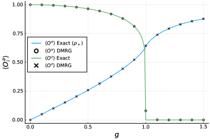
Figure 7: The expectation values $\langle O_{i}^{z}\rangle\equiv\langle Z_{i}\rangle$ and $\langle O_{i}^{x}\rangle\equiv\langle X_{i}\rangle$ as a function of $g$ where $i$ is chosen to the site at the center of the lattice. The exact result using the density matrix $\rho$, as discussed in Appendix E, is shown as a solid line. The markers show the results obtained using dmrg with a pinning field on a lattice with $L=64$.

Appendix E Exact Results in the tfim

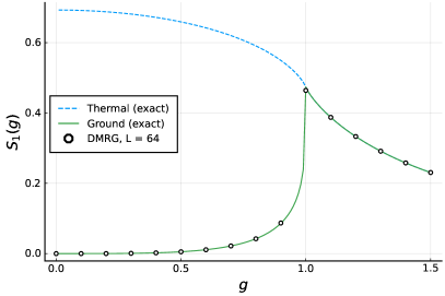
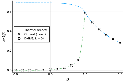
Figure 8: On the left panel, we show the single-site von Neumann entropy as a function of the coupling $g$ computed using the reduced density matrix $\rho^{r}_{i}$ of the ground state of the tfim, where $i$ is chosen to the site at the center of the lattice. As explained in the text, $\rho^{r}_{i}$ can be computed exactly using $\rho$ (solid line) or $\rho_{\rm th}$ (dashed line). The calculations using mps with $L=64$ are also shown as circles. On right panel, we show the two-site entanglement entropy as a function of $g$ computed using the reduced density matrix $\rho^{r}_{ij}$ of the ground state of the tfim, where $i,j$ are nearest neighbor sites at the center of the lattice. Again $\rho^{r}_{ij}$ can be computed using $\rho$ or $\rho_{\rm th}$. The exact answer obtained using $\rho_{\rm th}$ is known and is shown as the dashed line. The exact answer is not known for the ground state with a pinning field in the broken phase, but our answer obtained using mps is shown as circles.

In this section we wish to point out some subtleties in the calculation in the broken phase. First note that in our calculations we have assumed that the ground state of the Ising model is unique for all values of $g$ and $\rho$ is the density matrix for this unique ground state. However, as discussed in Section III and Appendix D, in the broken phase the ground state is doubly degenerate and we have to make a choice. We do this by introducing a small pinning field, taking the thermodynamic limit and then removing the pinning field. Thus, in our calculations $\rho$ corresponds to a single ground state density matrix for all values of $g$. In contrast one may in principle compute $\rho_{\rm th}$ to denote the thermal density matrix at zero temperature, which is different from $\rho$ in the broken phase since it is a density matrix of a mixed state with equal probabilities of being in both ground states. We want to be sure that the results we obtain using our mps approach in a finite volume with a small pinning field is from $\rho$ rather than $\rho_{\rm th}$. To confirm this, in this appendix we show our results for the von-Neumann entropy obtained from one-site and two-site reduced density matrices $\rho^{r}_{i}$ and $\rho^{r}_{ij}$ which are different depending on whether we use the $\rho$ or $\rho_{\rm th}$ to compute them and compare these results with exact results our dmrg calculations. For the tfim defined in Eq. 8 the expectation values

$$C^{a}=\mathrm{Tr}(\rho O^{a}_{i}),\ \ c^{a}=\mathrm{Tr}(\rho_{\rm th}O^{a}_{i}),$$ (47)

where $O^{x}_{i}=X_{i}$, $O^{y}_{i}=Y_{i}$ and $O^{z}_{i}=Z_{i}$, can be computed exactly. One can show that

$$C^{x} =\frac{1}{\pi}\int_{0}^{\pi}\!\!\!d\phi\ \frac{(g+\cos\phi)}{(\sin\phi)^{2}+(g+\cos\phi)^{2}},$$ (48)

$$C^{z} =\begin{cases}0&g\geq 1,\\ (1-g^{2})^{1/8}&g<1,\end{cases}$$ (49)

whereas $c^{x}=C^{x}$ and $c^{z}=0$. Thus, we see that $C^{z}$ is different in the broken phase. This difference affects the single-site density matrix, which is given by either

$$\rho^{r}_{i} =\frac{1}{2}(\mathbb{I}+C^{x}\sigma^{x}+C^{z}\sigma^{z})$$ (50)

or a similar expression where the $C$’s are replaced by $c$’s depending on whether we use $\rho$ or $\rho_{\rm th}$ in computing the coefficients. In the left plot of Fig. 8, we show how the single site von-Neumann entropy obtained using $S(g)=Tr(\rho_{i}^{r}\ln(\rho^{r}_{i}))$ differs from $\rho$ and $\rho_{\rm th}$. The difference is only present in the broken phase $g<1$. Our dmrg results agree with those calculated using $\rho$.

In the right plot of Fig. 8, we plot the two-site von Neumann entropy obtained from the two site reduced density matrix $\rho^{r}_{ij}$ where $|i-j|=1$ and $i,j$ are chosen at the center of the lattice to minimize finite size effects. We again notice that the difference between calculating $\rho^{r}_{ij}$ using $\rho$ or $\rho_{\rm th}$ in the broken phase ($g<1$) and our dmrg results agree with those calculated using $\rho$. The exact results shown were computed using the formula known in the literature [61], where

$$\rho^{r}_{ij} =\frac{1}{4}\textstyle\sum_{\mu,\nu}\ C^{\mu\nu}_{ij}\sigma^{\mu}\otimes\sigma^{\nu}.$$ (51)

where the two point correlation functions

$$C^{ab}_{ij}=\mathrm{Tr}(\rho O^{a}_{i}O^{b}_{j}),$$ (52)

have been computed using the density matrix $\rho$. We use a similar expression to compute the thermal reduced density matrix, but $C^{\mu\nu}_{ij}$ are replaced by $c^{\mu\nu}_{ij}$ computed using $\rho_{\rm th}$ instead of $\rho$. In Eq. 51 we allow $\mu,\nu=0,\dotsc,3$ and $\sigma^{0}=\mathbb{I}$ and $\sigma^{i},i=1,2,3$ are the Pauli matrices. Note that the correlation functions $C^{\mu\nu}_{ij}$ and $c^{\mu\nu}_{ij}$ depend only on $|i-j|$ and are symmetric under the exchange $a\leftrightarrow b$. The diagonal ones can be evaluated exactly in terms of the function $G(r)$ given by

$$G(r)=\frac{1}{\pi}\int_{0}^{\pi}\!\!\!\!d\phi\ \frac{(\cos(\phi r)(g+\cos\phi)-\sin(\phi r)\sin\phi}{\sqrt{(\sin\phi)^{2}+(g+\cos\phi)^{2}}}.$$ (53)

In particular we can show

$$C^{xx}_{ij} =C_{i}^{x}C_{j}^{x}-G(i-j)G(j-i)$$ (54)

$$C^{yy}_{ij} =\det{\tilde{\mathsf{G}}}^{[r]}$$ (55)

$$C^{zz}_{ij} =\det{\mathsf{G}}^{[r]}.$$ (56)

where we have defined $r\times r$ matrices ${\mathsf{G}}^{[r]}$ and ${\tilde{\mathsf{G}}}^{[r]}$ as

$${\mathsf{G}}_{a,b}^{[r]}=G(a-b-1)$$ (57)

$${\tilde{\mathsf{G}}}_{a,b}^{[r]}=G(a-b+1).$$ (58)

In the notation above, $a,b=1,\dotsc,r$ and $r=|i-j|$ represents the distance between the sites. Note further that $C^{00}_{ij}=1$, $C^{0a}_{ij}=C^{a}_{i}=C^{a}_{j}$ and $C^{xy}_{ij}=C^{yz}_{ij}=0$. The mixed correlation function $C^{xz}_{ij}\neq 0$ in the broken phase and unfortunately it is not easy to obtain this function analytically. Further $C^{ab}_{ij}=c^{ab}_{ij}$ in all cases except for the fact that $c^{xz}_{ij}=0$ for all values of $g$ unlike $C^{xz}_{ij}$ . Therefore, calculations for the reduced density matrix $\rho^{r}_{ij}$, will differ between the thermal ensemble and the fixed ground state with a pinning field. In our calculations we compute $C^{xz}_{ij}$ using dmrg and plug it into the expressions in Eq. 51, but use analytical expressions for all other correlation functions.

In Fig. 2 we showed our results for the two-site entanglement negativity ${\cal N}(\rho^{r}_{ij})$ (with $b=1$) that we obtained using dmrg and compared it with the exact results computed in Ref. [61]. We also observed that the negativity did not depend on whether we used $\rho$ or $\rho_{\rm th}$ in our calculations. We later discovered the reason for this is that the partial transpose of $\rho^{r}_{ij}$ required during the calculation of the ${\cal N}(\rho^{r}_{ij})$ simply corresponds to setting $C^{yy}_{ij}\mapsto-C^{yy}_{ij}$ (or $c^{yy}_{ij}\mapsto-c^{yy}_{ij}$. This leads to only one negative eigenvalue of the partial transpose which is also the negativity, and is given by

$${\cal N}(\rho^{r}_{ij})=\frac{1}{4}(1-C^{xx}_{ij}+C^{yy}_{ij}-C^{zz}_{ij}).$$ (59)

Since this is independent of $C^{z}$ as well as $C^{xz}_{ij}$, the negativity is the same for both the thermal and the single ground state density matrices. In other words, the two-point negativity is the same for both $\rho_{+}$ and $\rho_{\mathrm{th}}$, even though the von Neumann entropy is different in the broken phase.

Appendix F Aligning Density Matrices

A maximally entangled 2-qubit state can be constructed as

$$\mathclose{\,\mathopen{|}\mathord{\theta,\phi,\beta}\mathclose{\rangle}}=(R^{\dagger}_{\theta,\phi,\beta}\otimes R_{\theta,\phi,\beta})(\mathclose{\,\mathopen{|}\mathord{\uparrow}\mathclose{\rangle}}\otimes\mathclose{\,\mathopen{|}\mathord{\downarrow}\mathclose{\rangle}}-\mathclose{\,\mathopen{|}\mathord{\downarrow}\mathclose{\rangle}}\otimes\mathclose{\,\mathopen{|}\mathord{\uparrow}\mathclose{\rangle}})\,,$$ (60)

where the $SU(2)$ rotation matrix is parameterized as

$$R_{\theta,\phi,\beta} =\begin{pmatrix}e^{i\phi}\cos\theta&-ie^{i\beta}\sin\theta\\ -ie^{-i\beta}\sin\theta&e^{-i\phi}\cos\theta\end{pmatrix}\,,$$ (61)

Hence, we see that two density matrices can be maximally entangled but their average can be less entangled because these density matrices are aligned differently. This can lead to a loss of entanglement in the symmetrization step we discussed earlier in Appendix B. A way to check how close a density matrix $\rho$ is to a maximally entangled state is to measure the maximal singlet fraction $F_{m}(\rho)=\mathopen{\mathopen{\langle}\mathord{\theta,\phi,\beta}\mathclose{|}\,}\rho\mathclose{\,\mathopen{|}\mathord{\theta,\phi,\beta}\mathclose{\rangle}}$ [81], which is nothing but the maximal fidelity of the given density matrix to any maximally entangled state Bennett et al. [82].

Note that since the diagonal subgroup of $U(2)\otimes U(2)$ leaves the singlet invariant, we can use $I\otimes R_{\theta,\phi,\beta}^{2}$ instead of $R_{\theta,\phi,\beta}^{\dagger}\otimes R_{\theta,\phi,\beta}$. In addition to the periodicities in $\theta\to\theta+\pi$, $\phi\to\phi+2\pi$, and $\beta\to\beta+2\pi$, the rotation matrix $R_{\theta,\phi,\beta}^{2}$ has the following properties:

$$R_{\theta,\phi,\beta}^{2} =-R_{\theta+\pi/2,\phi,\beta}^{2}$$

$$=R_{-\theta,\phi,\beta+\pi}^{2}$$

$$=R_{\theta,\phi+\pi,\beta+\pi}^{2}\,.$$ (62)

Since the phase of the state is irrelevant in this calculation, the region $\theta\in[0,\pi/4\mathclose{[}$, $\phi\in\mathopen{]}-\pi/2,\pi/2]$, $\beta\in\mathopen{]}-\pi,\pi]$ contains all the independent maximally entangled density matrices. Thus, the fidelity can be numerically maximized within this domain.

Given a density matrix $\rho$ and the rotation angles $\theta,\phi,\beta$ that maximises the singlet fraction $F_{m}(\rho)$, we can construct a new aligned density matrix $\rho^{A}=U^{\dagger}_{A}\rho U_{A}$ such that the rotation angles $\theta=0,\phi=0,\beta=0$ maximizes its singlet fraction. These aligned density matrices can then be used while symmetrizing the density matrix.

References

- Witten [2018] E. Witten, APS medal for exceptional achievement in research: Invited article on entanglement properties of quantum field theory, Rev. Mod. Phys. 90, 045003 (2018).
- Reeh and Schlieder [1961] H. Reeh and S. Schlieder, Bemerkungen zur Unitäräquivalentz von lorentzvarianten Feldern, Nuovo Cimento 22, 1051 (1961).
- Schlieder [1965] S. Schlieder, Some remarks about the localization of states in a quantum field theory, Communications in Mathematical Physics 1, 265 (1965).
- Unruh [1976] W. G. Unruh, Notes on black-hole evaporation, Phys. Rev. D 14, 870 (1976).
- Summers and Werner [1985] S. J. Summers and R. Werner, The vacuum violates Bell’s inequalities, Physics Letters A 110, 257 (1985).
- Summers and Werner [1987a] S. J. Summers and R. Werner, Bell’s inequalities and quantum field theory. I. General setting, Journal of Mathematical Physics 28, 2440 (1987a).
- Summers and Werner [1987b] S. J. Summers and R. Werner, Bell’s inequalities and quantum field theory. II. Bell’s inequalities are maximally violated in the vacuum, Journal of Mathematical Physics 28, 2448 (1987b).
- Redhead [1995] M. Redhead, More ado about nothing, Foundations of Physics 25, 123 (1995).
- Redhead and Wagner [1998] M. L. G. Redhead and F. Wagner, Unified treatment of EPR and Bell arguments in algebraic quantum field theory, Foundations of Physics Letters 11, 111 (1998).
- Clifton et al. [1998] R. Clifton, D. V. Feldman, H. Halvorson, M. L. G. Redhead, and A. Wilce, Superentangled states, Phys. Rev. A 58, 135 (1998).
- Cardy [2008] J. L. Cardy, Entanglement entropy in extended quantum systems, Eur. Phys. J. B 64, 321 (2008).
- Amico et al. [2008] L. Amico, R. Fazio, A. Osterloh, and V. Vedral, Entanglement in many-body systems, Rev. Mod. Phys. 80, 517 (2008).
- Kitaev and Preskill [2006] A. Kitaev and J. Preskill, Topological entanglement entropy, Phys. Rev. Lett. 96, 110404 (2006).
- Levin and Wen [2006] M. Levin and X.-G. Wen, Detecting topological order in a ground state wave function, Phys. Rev. Lett. 96, 110405 (2006).
- Calabrese and Cardy [2005] P. Calabrese and J. Cardy, Evolution of entanglement entropy in one-dimensional systems, Journal of Statistical Mechanics: Theory and Experiment 2005, P04010 (2005).
- Ho and Abanin [2017] W. W. Ho and D. A. Abanin, Entanglement dynamics in quantum many-body systems, Phys. Rev. B 95, 094302 (2017).
- Wen [1990] X. G. Wen, Topological order in rigid states, Int. J. Mod. Phys. B 4, 239 (1990).
- Cirac et al. [2020] I. Cirac, D. Perez-Garcia, N. Schuch, and F. Verstraete, Matrix Product States and Projected Entangled Pair States: Concepts, symmetries, and theorems (2020), arXiv:2011.12127 [cond-mat, physics:hep-th, physics:quant-ph] .
- Nielsen and Chuang [2000] M. A. Nielsen and I. L. Chuang, Quantum Computation and Quantum Information (Cambridge University Press, 2000).
- Bennett et al. [1993] C. H. Bennett, G. Brassard, C. Crépeau, R. Jozsa, A. Peres, and W. K. Wootters, Teleporting an unknown quantum state via dual classical and Einstein-Podolsky-Rosen channels, Physical Review Letters 70, 1895 (1993).
- Valentini [1991] A. Valentini, Non-local correlations in quantum electrodynamics, Physics Letters A 153, 321 (1991).
- Reznik et al. [2005] B. Reznik, A. Retzker, and J. Silman, Violating Bell’s inequalities in vacuum, Phys. Rev. A 71, 042104 (2005).
- Reznik [2003] B. Reznik, Entanglement from the vacuum, Foundations of Physics 33, 167 (2003).
- Reznik [2000] B. Reznik, Distillation of vacuum entanglement to EPR pairs (2000), arXiv:quant-ph/0008006 .
- Brown [2013] E. G. Brown, Thermal amplification of field-correlation harvesting, Physical Review A 88, 062336 (2013).
- Braun [2005] D. Braun, Entanglement from thermal blackbody radiation, Physical Review A 72, 062324 (2005).
- Braun [2002] D. Braun, Creation of Entanglement by Interaction with a Common Heat Bath, Physical Review Letters 89, 277901 (2002).
- Simidzija and Martín-Martínez [2017] P. Simidzija and E. Martín-Martínez, Nonperturbative analysis of entanglement harvesting from coherent field states, Physical Review D 96, 065008 (2017).
- Pozas-Kerstjens and Martín-Martínez [2016] A. Pozas-Kerstjens and E. Martín-Martínez, Entanglement harvesting from the electromagnetic vacuum with hydrogenlike atoms, Physical Review D 94, 064074 (2016).
- Pozas-Kerstjens and Martín-Martínez [2015] A. Pozas-Kerstjens and E. Martín-Martínez, Harvesting correlations from the quantum vacuum, Physical Review D 92, 064042 (2015).
- Maeso-García et al. [2022] H. Maeso-García, T. R. Perche, and E. Martín-Martínez, Entanglement harvesting: Detector gap and field mass optimization, Physical Review D 106, 045014 (2022).
- Salton et al. [2015] G. Salton, R. B. Mann, and N. C. Menicucci, Acceleration-assisted entanglement harvesting and rangefinding, New Journal of Physics 17, 035001 (2015).
- Sachs et al. [2017] A. Sachs, R. B. Mann, and E. Martín-Martínez, Entanglement harvesting and divergences in quadratic Unruh-DeWitt detector pairs, Physical Review D 96, 085012 (2017).
- Steeg and Menicucci [2009] G. V. Steeg and N. C. Menicucci, Entangling power of an expanding universe, Physical Review D 79, 044027 (2009).
- Martín-Martínez et al. [2016] E. Martín-Martínez, A. R. H. Smith, and D. R. Terno, Spacetime structure and vacuum entanglement, Physical Review D 93, 044001 (2016).
- Gühne and Tóth [2009] O. Gühne and G. Tóth, Entanglement detection, Physics Reports 474, 1 (2009).
- Vidal and Werner [2002] G. Vidal and R. F. Werner, Computable measure of entanglement, Physical Review A 65, 032314 (2002).
- Shapourian et al. [2017] H. Shapourian, K. Shiozaki, and S. Ryu, Partial time-reversal transformation and entanglement negativity in fermionic systems, Physical Review B 95, 165101 (2017).
- Shapourian and Ryu [2019] H. Shapourian and S. Ryu, Finite-temperature entanglement negativity of free fermions, Journal of Statistical Mechanics: Theory and Experiment 2019, 043106 (2019).
- Cornfeld et al. [2019] E. Cornfeld, E. Sela, and M. Goldstein, Measuring Fermionic Entanglement: Entropy, Negativity, and Spin Structure, Physical Review A 99, 062309 (2019), arXiv:1808.04471 .
- Chang and Wen [2016] P.-Y. Chang and X. Wen, Entanglement negativity in free-fermion systems: An overlap matrix approach, Physical Review B 93, 195140 (2016).
- Audenaert et al. [2002] K. Audenaert, J. Eisert, M. B. Plenio, and R. F. Werner, Entanglement Properties of the Harmonic Chain, Physical Review A 66, 042327 (2002), arXiv:quant-ph/0205025 .
- Klco and Savage [2021a] N. Klco and M. J. Savage, Geometric quantum information structure in quantum fields and their lattice simulation, Phys. Rev. D 103, 065007 (2021a).
- Klco and Savage [2021b] N. Klco and M. J. Savage, Entanglement spheres and a UV-IR connection in effective field theories (2021b), arXiv:2103.14999 [hep-th] .
- Klco et al. [2021] N. Klco, D. H. Beck, and M. J. Savage, Entanglement structures in quantum field theories: Negativity cores and bound entanglement in the vacuum (2021), arXiv:2110.10736 [quant-ph] .
- Ruggiero et al. [2016] P. Ruggiero, V. Alba, and P. Calabrese, Negativity spectrum of one-dimensional conformal field theories, Physical Review B 94, 195121 (2016), arXiv:1607.02992 .
- Calabrese et al. [2014] P. Calabrese, J. Cardy, and E. Tonni, Finite temperature entanglement negativity in conformal field theory, Journal of Physics A: Mathematical and Theoretical 48, 015006 (2014).
- Calabrese et al. [2013] P. Calabrese, L. Tagliacozzo, and E. Tonni, Entanglement negativity in the critical Ising chain, Journal of Statistical Mechanics: Theory and Experiment 2013, P05002 (2013).
- Calabrese et al. [2012] P. Calabrese, J. Cardy, and E. Tonni, Entanglement negativity in quantum field theory, Physical Review Letters 109, 130502 (2012), arXiv:1206.3092 .
- Wen et al. [2015] X. Wen, P.-Y. Chang, and S. Ryu, Entanglement negativity after a local quantum quench in conformal field theories, Physical Review B 92, 075109 (2015).
- Hoogeveen and Doyon [2015] M. Hoogeveen and B. Doyon, Entanglement negativity and entropy in non-equilibrium conformal field theory, Nuclear Physics B 898, 78 (2015).
- Eisler and Zimborás [2014] V. Eisler and Z. Zimborás, Entanglement negativity in the harmonic chain out of equilibrium, New Journal of Physics 16, 123020 (2014).
- Peres [1996] A. Peres, Separability criterion for density matrices, Phys. Rev. Lett. 77, 1413 (1996).
- Horodecki et al. [1995] R. Horodecki, P. Horodecki, and M. Horodecki, Violating Bell inequality by mixed spin-12 states: Necessary and sufficient condition, Physics Letters A 200, 340 (1995).
- Ha and Kye [2011] K.-C. Ha and S.-H. Kye, Entanglement witnesses arising from exposed positive linear maps, Open Systems & Information Dynamics 18, 323 (2011).
- Skowronek [2016] Ł. Skowronek, There is no direct generalization of positive partial transpose criterion to the three-by-three case, Journal of Mathematical Physics 57, 112201 (2016).
- Horodecki et al. [1998a] M. Horodecki, P. Horodecki, and R. Horodecki, Mixed-state entanglement and distillation: Is there a “bound” entanglement in nature?, Physical Review Letters 80, 5239 (1998a).
- Horodecki et al. [1999] P. Horodecki, M. Horodecki, and R. Horodecki, Bound entanglement can be activated, Phys. Rev. Lett. 82, 1056 (1999), arXiv:quant-ph/9806058 .
- Stinchcombe [1973] R. B. Stinchcombe, Ising model in a transverse field. I. basic theory, Journal of Physics C: Solid State Physics 6, 2459 (1973).
- Sachdev [2011] S. Sachdev, Quantum Phase Transitions, 2nd ed. (Cambridge University Press, 2011).
- Osborne and Nielsen [2002] T. J. Osborne and M. A. Nielsen, Entanglement in a simple quantum phase transition, Physical Review A 66, 032110 (2002), arXiv:quant-ph/0202162 .
- Osterloh et al. [2002] A. Osterloh, L. Amico, G. Falci, and R. Fazio, Scaling of entanglement close to a quantum phase transitions, Nature 416, 608 (2002), arXiv:quant-ph/0202029 .
- Roos [1970] H. Roos, Independence of local algebras in quantum field theory, Communications in Mathematical Physics 16, 238 (1970).
- Buchholz [1974] D. Buchholz, Product states for local algebras, Communications in Mathematical Physics 36, 287 (1974).
- Alba [2013] V. Alba, Entanglement negativity and conformal field theory: A Monte Carlo study, Journal of Statistical Mechanics: Theory and Experiment 2013, P05013 (2013).
- Yu and Eberly [2009] T. Yu and J. H. Eberly, Sudden death of entanglement, Science 323, 598 (2009).
- Bhattacharyya [1943] A. K. Bhattacharyya, On a measure of divergence between two statistical populations defined by their probability distributions, Bulletin of the Calcutta Mathematical Society 35, 99 (1943).
- Matusita [1971] K. Matusita, Some properties of affinity and applications, Annals of the Institute of Statistical Mathematics 23, 137 (1971).
- Hudson and Moody [1976] R. L. Hudson and G. R. Moody, Locally normal symmetric states and an analogue of de Finetti’s theorem, Zeitschrift für Wahrscheinlichkeitstheorie und verwandte Gebiete 33, 343 (1976).
- Caves et al. [2002] C. M. Caves, C. A. Fuchs, and R. Schack, Unknown quantum states: The quantum de Finetti representation, Journal of Mathematical Physics 43, 4537 (2002) [Erratum: ibid. 49, 019902 (2002)], arXiv:quant-ph/0104088 .
- Verstraete and Verschelde [2002] F. Verstraete and H. Verschelde, Fidelity of mixed states of two qubits, Phys. Rev. A 66, 022307 (2002), quant-ph/0203073 .
- Schauss [2018] P. Schauss, Quantum simulation of transverse Ising models with Rydberg atoms, Quantum Science and Technology 3, 023001 (2018).
- Semeghini et al. [2021] G. Semeghini, H. Levine, A. Keesling, S. Ebadi, T. T. Wang, D. Bluvstein, R. Verresen, H. Pichler, M. Kalinowski, R. Samajdar, A. Omran, S. Sachdev, A. Vishwanath, M. Greiner, V. Vuletić, and M. D. Lukin, Probing topological spin liquids on a programmable quantum simulator, Science 374, 1242 (2021).
- Fishman et al. [2022a] M. Fishman, S. R. White, and E. M. Stoudenmire, Codebase release 0.3 for ITensor, SciPost Phys. Codebases , 4 (2022a).
- Fishman et al. [2022b] M. Fishman, S. R. White, and E. M. Stoudenmire, The ITensor software library for tensor network calculations, SciPost Phys. Codebases , 4 (2022b).
- Brandt [1999] H. E. Brandt, Positive operator valued measure in quantum information processing, American Journal of Physics 67, 434 (1999).
- Casini et al. [2014] H. Casini, M. Huerta, and J. A. Rosabal, Remarks on entanglement entropy for gauge fields, Phys. Rev. D 89, 085012 (2014), arXiv:1312.1183 [hep-th] .
- Schollwöck [2011] U. Schollwöck, The density-matrix renormalization group in the age of matrix product states, Annals of Physics January 2011 Special Issue, 326, 96 (2011).
- White [1992] S. R. White, Density matrix formulation for quantum renormalization groups, Physical Review Letters 69, 2863 (1992).
- White [1993] S. R. White, Density-matrix algorithms for quantum renormalization groups, Physical Review B 48, 10345 (1993).
- Horodecki et al. [1998b] M. Horodecki, P. Horodecki, and R. Horodecki, General teleportation channel, singlet fraction and quasidistillation (1998b), arXiv:quant-ph/9807091 .
- Bennett et al. [1996] C. H. Bennett, D. P. DiVincenzo, J. A. Smolin, and W. K. Wootters, Mixed state entanglement and quantum error correction, Phys. Rev. A 54, 3824 (1996), arXiv:quant-ph/9604024 .