A DeepONet multi-fidelity approach for residual learning in reduced order modeling

Abstract

In the present work, we introduce a novel approach to enhance the precision of reduced order models by exploiting a multi-fidelity perspective and DeepONets. Reduced models provide a real-time numerical approximation by simplifying the original model. The error introduced by the such operation is usually neglected and sacrificed in order to reach a fast computation. We propose to couple the model reduction to a machine learning residual learning, such that the above-mentioned error can be learned by a neural network and inferred for new predictions. We emphasize that the framework maximizes the exploitation of high-fidelity information, using it for building the reduced order model and for learning the residual. In this work, we explore the integration of proper orthogonal decomposition (POD), and gappy POD for sensors data, with the recent DeepONet architecture. Numerical investigations for a parametric benchmark function and a nonlinear parametric Navier-Stokes problem are presented.

1 Introduction

Multi-fidelity (MF) methods emerged as a solution to deal with complex models, which usually need a high computational budget to be solved [58]. Such a framework aims to exploit not only the so-called high-fidelity information, but also the response of low-fidelity models in order to increase the accuracy of the prediction. This feature plays a fundamental role, especially for outer loop applications such as uncertainty propagation and optimization, since it allows to achieve good accuracy without requiring evaluating the high-fidelity model (typically expensive) at every iteration. Thus, its employment is widespread for optimization purposes, and among all the contributions in literature, we highlight the successful application to naval engineering problems [13, 12, 69], to multiple fidelities modeling [28], and in the presence of uncertainty [54]. All these cases, as well as many others, build the correlation between the different fidelities by involving Gaussian process regression (GPR). Another approach with nonlinear autoregressive schemes is described in [59, 62], whereas in [64] a possible extension for high-dimensional parameter spaces is investigated. Recently, an alternative to such a probabilistic framework is offered by neural networks, where the mapping between the low-fidelity model and the high-fidelity one is learned by the network during the training procedure [79, 51, 33]. Among the different types of architecture, DeepONet [44, 41] has been proposed to approximate operators and it has been successfully applied to MF problems in [45, 37]. It has also been successfully used to create a fast PDE-constrained optimization method in [73]. Another type of architecture that has been successfully applied to multi-fidelity data is the Bayesian neural network [50], resulting in a framework robust to noisy measurements. We also highlight the employment of multi-fidelity techniques for uncertainty quantification. We cite [35, 34] for a Bayesian framework capable to deal with model discrepancy using different fidelities, whereas we refer to [27] for an analysis of the trade-off between high- and low-fidelity data in a Monte Carlo estimation.

Reduced order modeling (ROM) [10, 19, 65] is a family of methods that aims at reducing the computational burden of evaluating complex models. Instead of combining data from heterogeneous models, ROM builds a simplified model, typically from some high-fidelity information. Also, in this case, the capabilities of ROM led to its diffusion in several industrial contexts [52, 69, 67], especially for optimization tasks [11, 3, 78, 70, 25, 22] or inverse problems [31, 38]. In the ROM community, proper orthogonal decomposition (POD) is one of the most employed methods to build the reduced model [60, 61, 7, 8, 9]. Given a limited set of high-fidelity data, POD is able to compute the reduced space of an arbitrary rank which optimally (in a least squares sense) represents the data. In the last years, its diffusion led to several variants including shifted POD [56, 63], weighted POD [18, 71], and gappy POD [26, 75, 17, 46]. This latter exploit a compressive sensing approach [14, 16, 40], in order to use only a few information at certain locations of the domain (sensors) to compute the approximation. A generalization of gappy POD can be found in [1], where linear stochastic estimation allows the reconstruction of the linear map between the available data and the system state by an $l_{2}$ minimization. A novel approach where such a relation between sensor data and the reduced state is approximated in a nonlinear way employing neural networks can be found in [53].

In the present contribution, we explore the possibility of coupling these two methodologies, MF and ROM, to enhance the accuracy of the model. ROM indeed creates a simplified model from a few high-fidelity data. Such approximation can be considered the low-fidelity model, because of the projection error introduced by the ROM. In this context, MF could be adopted in order to find the correlation between the original model and the ROM one, resulting in a more precise prediction. We can therefore exploit twice the collected high-fidelity data: initially, it is used to build the reduced model, then again during the computation of the MF relation. From this point of view, the proposed improvement does not need any additional high-fidelity evaluations. Here we take into consideration the POD with interpolation or the gappy POD as low-fidelity modeling techniques and the DeepONet to learn the residual. POD with interpolation [74, 68, 29, 24] is applied here for a completely data-driven approach, while gappy POD is used in order to make the pipeline applicable even for sensor data. The framework aims then to exploit the capability of POD models for linear prediction, adding the nonlinear term through the DeepONet, which can be viewed as a data-driven closure model. See [76] for another data-driven modelling approach to close ROMs, while for other recent works that propose nonlinear model order reduction, we cite [4, 2, 39, 66, 30, 49, 42].

The manuscript is organized as follows. In Section 2 we present the end-to-end numerical pipeline, with a focus on POD, gappy POD, and DeepONets. We continue in Section 3 by showing the numerical experiments, and finally we conclude with Section 4 by summarizing the results and drawing some future extensions.

2 Methods

This section is devoted to present the numerical methods used within the proposed approximation scheme, together with the methods used for comparison. We describe their integration in order to provide a global overview, then we discuss in the following sections the algorithmic details.

Proper orthogonal decomposition (POD) is a widespread technique providing a linear model order reduction, particularly suited to deal with parametric problems [65, 48, 20]. Such a representation is computationally very cheap to acquire, however, it suffers from the linear limitations of POD that may decrease its accuracy, especially when dealing with nonlinear problems.

We are interested in efficiently computing a parametric field $\mathbf{u}(\mu)$ with $\mathbf{u}:P\to\mathcal{V}$, where $P$ is the parametric space, $\mathcal{V}$ a generic norm equipped vector space with $\text{dim}(\mathcal{V})=n$. POD-based ROMs compute the approximation $\mathbf{u}_{\text{POD}}(\mu)$ such that:

$$\mathbf{u}_{\text{POD}}(\mu)\approx\mathbf{u}(\mu)=\mathbf{u}_{\text{POD}}(\mu)+\mathbf{r}(\mu),$$ (1)

where $\mathbf{r}:P\to\mathcal{V}$ is the projection error introduced by the model order reduction, which we assume here to be dependent on the parameter. In a classical POD framework, this residual $\mathbf{r}$ is usually neglected, due to its marginal contribution. In the present contribution, we aim instead to learn it by means of machine learning techniques, in order to improve the accuracy of the final prediction. Artificial neural networks (ANNs) can be used to model it, thanks to their general approximation capabilities, learning it by exploiting the snapshots already pre-computed to build the ROM. In particular, dealing with parametric problems, we exploit the DeepONet architecture to learn the residual. The light computational demand to infer the DeepONet enables a nonlinear but still real-time improvement of the POD model, at the cost of additional training during the offline phase.

The only input needed by the proposed methodology is the numerical solutions database $\{\mu_{i},\mathbf{u}(\mu_{i})\}_{i=1}^{N}$ computed by sampling the parameter space and exploiting any consolidated discretization method (e.g. finite element or finite volume method). These snapshots are combined in order to find the POD space, which can be used for intrusive or non-intrusive ROM. We explore in this contribution only the non-intrusive (data-driven) approach, while future works will study the application to POD-Galerkin contexts. We investigate two options for the non-intrusive ROM:

• POD with radial basis functions (POD-RBF) interpolation, which enables the prediction of new solutions (for new parameters) by means of the above-mentioned interpolation technique. In this case, the ROM takes as input the actual parameter providing as output the approximated solution.

• Gappy POD, which allows us to compute the approximated solution by providing only some sensor data thanks to a compressing strategy.

Once the ROM is built, we can exploit it to compute the low-fidelity representation of the original snapshots by passing the corresponding parameters (or sensor data). The high-fidelity and low-fidelity databases are then used to learn the difference between them through the DeepONet network with the final aim of generalizing such residual even to unseen parameters and improving the final prediction. It is important to note that typically the space $\mathcal{V}$ is obtained by discretizing a generic $\mathbb{R}^{d}$ space. Depending on the complexity of the equation to solve and on the target accuracy, this kind of space can exhibit a high number of degrees of freedom.

Approximating the error over such a high-dimensional space with a neural network leads to two major issues: i.) the number of the neurons in the last layer is equal to the number of degrees of freedom of the space $\mathcal{V}$, resulting in a model too large to treat; ii.) the parameter-to-error relation becomes too complex to be efficiently learned. Thus we extract the spatial coordinates of the degrees of freedom of $\mathcal{V}$. Since we know the error (the difference between the original snapshots and the POD predictions) in any of these coordinates, we can arrange the data in the format $\{(x_{i},\mu_{j},\mathbf{r}(\mu_{j})_{i})\,|\,x_{i}\in\mathcal{V}\subset\mathbb{R}^{d},\mu_{j}\in P,\mathbf{r}(\mu_{j})_{i}\in\mathbb{R}\}$ where $i=1,\dots,n$ and $j=1,\dots,N$, to isolate the spatial and parametric dependency of the error. We can use such a dataset to learn the scalar error $r_{\text{net}}:\mathbb{R}^{d}\times P\to\mathbb{R}$ given the parametric and spatial coordinates. In this way, the network maintains a limited number of output dimensions, improving the identification of spatial recurrent patterns. The loss function which is minimized during the training procedure is then:

$$\mathcal{L}=\frac{1}{N}\sum_{i=1}^{N}\|\mathbf{r}_{\text{NN}}(\mu_{i})+\mathbf{u}_{\text{POD}}(\mu_{i})-\mathbf{u}(\mu_{i})\|^{2},$$ (2)

where $\mathbf{r}_{\text{NN}}(\mu)$ is not the high-dimensional output of a single network evaluation, but the array containing the result of the network inference for any spatial coordinates belonging to the discretized space such that $\mathbf{r}_{\text{NN}}(\mu)\equiv\begin{bmatrix}r_{\text{net}}(x_{1},\mu)&r_{\text{net}}(x_{2},\mu)&\dots&r_{\text{net}}(x_{n},\mu)\end{bmatrix}$, where $x_{i}\in\mathbb{R}^{d}$ for $i=1,\dots,n$. In the case of gappy POD, it is important to note that the DeepONet takes as input the sensors data and not the actual parameters. We emphasize that the DeepONet training does not need any additional high-fidelity solutions besides those already collected for the POD space construction.

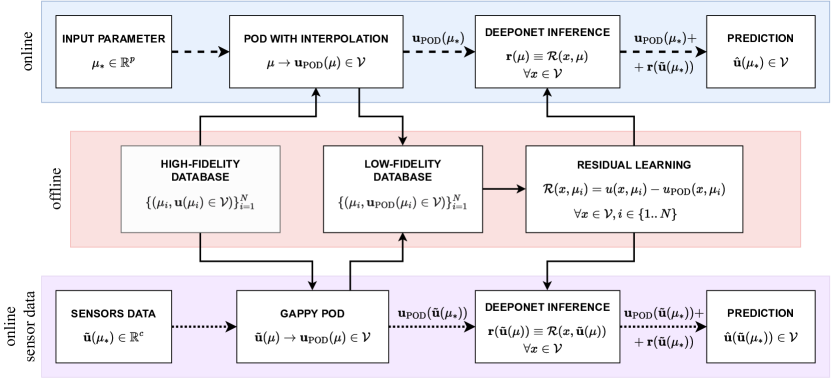
Figure 1: Scheme for the multi-fidelity POD framework. The arrows indicate the relationship between the different methods. In the blue box the dashed arrows indicate the online phase when the input parameter is provided. In the purple box the dotted arrows indicate the information flow if only sensor data are provided. The central red frame emphasizes the computationally expensive offline phase.

For the prediction of solutions for new parameters, the non-intrusive POD model and the DeepONet are finally queried, as sketched in Figure 1. POD returns the low-fidelity (linear) approximation by providing the test parameter or sensor data, while the neural network returns the nonlinear residual. In some sense, this pipeline aims to exploit the advantages of the consolidated POD model, but at the same time improves it by adding a nonlinear term. So it can be also seen as a closure model.

2.1 Proper Orthogonal Decomposition for low-fidelity modeling

POD is a consolidated technique widely used for model order reduction. In this section, we briefly introduce how to compute the POD modes, and we devote section 2.1.1 to present the gappy POD variant in detail.

The method consists of the computation of the optimal reduced basis to represent the parametric solution manifold through a linear projection. Let $u_{i}\in\mathbb{R}^{n}$ be the discrete solution corresponding to the $i$-th parameter, and $U=[u_{1},\dots,u_{N}]\in\mathbb{R}^{n\times N}$ be the snapshots matrix, whose columns are the solution vectors. We want to find a linear approximation such that:

$$u_{i}\approx\sum_{k=1}^{r}a_{i}^{k}\psi_{k},\qquad\text{ for }r\ll n,\text{ and for }i=1,\dots,N,$$ (3)

where $\psi_{i}\in\mathbb{R}^{n}$ are the vectors comprising the reduced basis, the so-called modes, and $a_{i}:=\begin{pmatrix}a_{i}^{1},a_{i}^{2},\dots,a_{i}^{r}\end{pmatrix}\in\mathbb{R}^{r}$ are the coordinates of the corresponding solution at the reduced level, called modal coefficients or latent variables. These reduced variables are obtained by a projection of the solution snapshots onto the modes.
The POD modes can be obtained from the matrix $U$ in different ways: by computing its singular value decomposition (SVD), or by decomposing its correlation matrix [72]. Moreover, all the modes have a corresponding singular value, which represents their energetic contribution. By arranging these modes in decreasing order (with respect to the singular values), we can express the original system with a hierarchical basis, from which we can discard the less meaningful modes. The energy criterion based on the singluar values decay reads as

$$\frac{\sum_{j=1}^{r}\sigma_{j}}{\sum_{j=1}^{N}\sigma_{j}}>\epsilon,$$ (4)

where $\sigma_{j}$ is the $j$-th singular value, and $\epsilon$ is a tolerance, usally set $\geq$0.99$$. In other words, by providing some samples of the solution manifold, POD is able to detect correlations between the data and reduce the dimensionality of these discrete solutions. This the approach becomes a fundamental tool for solving parametric partial differential equations (PDEs) in a many-query context, mainly due to the high-dimensional discrete spaces involved.

The POD space can be exploited in a Galerkin framework, by projecting the differential operators, or in a data-driven fashion by coupling it with an interpolation (or regression) technique. In this case, the database of reduced snapshots $\{\mu_{i},a_{i}\}_{i=1}^{N}$ is used as input to build the mapping $\mathcal{I}:P\to\mathbb{R}^{r}$ such that $\mathcal{I}(\mu_{i})=a_{i}$ for $i=1,\dots,N$, which is used for interpolating the modal coefficients for any new parameter. Depending on the chosen regression technique, the equality could not hold in principle, and we have $\mathcal{I}(\mu_{i})\approx a_{i}$. Finally, exploiting such a mapping, we have the possibility to query for the modal coefficients at any test parameter belonging to the space $P$ and finally exploit the POD modes to map back the approximated solution in the original high-dimensional space.

2.1.1 Gappy POD for sensors data

The main assumption for using gappy POD is to have access to only some sensor data. These sensors are placed at specific locations, given by the projection matrix, or point measurement matrix, $C\in\mathbb{R}^{c\times n}$, with $c\ll n$, which contains $1$ at measurements location and $0$ elsewhere. Using the canonical basis vectors of $\mathbb{R}^{n}$ it takes the following form

$$C=\begin{bmatrix}e_{\gamma_{1}}&e_{\gamma_{2}}&\cdots&e_{\gamma_{c}}\end{bmatrix}^{T},$$ (5)

for some indices $\gamma_{i}\in[1,\dots,n]$, with $i\in[1,\dots,c]$. The measurements $\tilde{u}_{*}\in\mathbb{R}^{c}$ of a generic full state vector $u_{*}\in\mathbb{R}^{n}$ are thus given by

$$\tilde{u}_{*}=Cu_{*}.$$ (6)

If we now consider a parametric framework we can collect the parameter–solution snapshot pairs $\{\mu_{i},u_{i}\}_{i=1}^{N}$, where $\mu_{i}\in P\subset\mathbb{R}^{p}$, and $u_{i}\in\mathbb{R}^{n}$ is the corresponding full state. We arrange the snapshots by column in $U$ as

$$U=\left[\begin{array}[]{cccc}|&|&|&|\\ u_{1}&u_{2}&\dots&u_{N}\\ |&|&|&|\end{array}\right].$$ (7)

We take the $r$-rank SVD of the snapshots matrix $U$ and compute the POD modes $\Psi_{r}$, so we can project the full states to their low-rank representation $a\in\mathbb{R}^{r\times N}$:

$$U=\Psi\Sigma V^{T}\approx\Psi_{r}\Sigma_{r}V_{r}^{T},\qquad U\approx\Psi_{r}a.$$ (8)

In the classical POD setting, where we deal with the full snapshots, we would just use the modal coefficients matrix $a$ to describe the solution manifold. For the gappy POD, instead, we have to consider the point measurement matrix. So, putting all together we have

$$\tilde{U}\approx(C\Psi_{r})a,$$ (9)

where $\tilde{U}$ is the matrix containing the sensors measurements $\{\tilde{u}_{i}\}_{i=1}^{N}$ arranged by columns, as done for the snapshots matrix. For a generic snapshot $\tilde{u}_{i}$ we have:

$$\tilde{u}_{i}\approx C\sum_{k=1}^{r}a_{i}^{k}\psi_{k},$$ (10)

where $\psi_{k}$ are the columns of $\Psi_{r}$, and $a_{i}^{k}$ are the modal coefficients, that is the $i$-th column of $a$. A possible solution to find the modal coefficients is to minimize the residual in a least-squares sense using the $L^{2}$ norm over the sensors locations which means considering the following quantity [15]

$$\int_{\text{supp}[\tilde{u}_{i}]}\left(\tilde{u}_{i}-\sum_{k=1}^{r}\tilde{a}_{i}^{k}\psi_{k}\right)^{2}.$$ (11)

There are many ways in the literature to select the locations of the sensors: optimal sensor locations that improve the condition number of $C\Psi$ [75, 47], which are robust to sensor noise, the sample maximal variance positions [77], or using information contained in secant vectors between data points [55], for example. In this work, we are going to use the sparse sensor placement optimization for reconstruction described in details in [47] and implemented in PySensors [21]. The main idea is to find $C$ that minimizes the reconstruction error using the modes $\Psi_{r}$ as in the following

$$C^{*}=\operatorname*{\arg\!\min}_{C}\|U-\Psi_{r}(C\Psi_{r})^{\dagger}\tilde{U}\|^{2}_{2},$$ (12)

where the symbol $\dagger$ stands for the Moore-Penrose pseudoinverse.

2.2 DeepONet for residual learning

DeepONet [44] is a neural network architecture able to learn nonlinear operators. Referring to the original work for all the details, we emphasize its architecture composed by two separate networks whose final outputs are multiplied to obtain the final DeepONet outcome. The two networks, called trunk and branch, can be any available architecture — e.g. convolutional network, graph network —. In this work we consider feedforward networks (FFNs). The networks are trained simultaneously during the learning loop: the input is indeed divided into two independent components, $x\in\mathbb{R}^{N_{x}}$ and $y\in\mathbb{R}^{N_{y}}$, which feed the two networks $NN_{x}$ and $NN_{y}$, respectively. The outputs $NN_{x}(x),NN_{y}(y)\in\mathbb{R}^{N_{p}}$ are finally multiplied to approximate the operator $\mathcal{G}$:

$$\mathcal{G}(x)(y)\approx\sum_{i=1}^{p}[NN_{x}(x)]_{i}[NN_{y}(y)]_{i}.$$ (13)

We underline that the choice of the two networks must satisfy the dimensional constraint: they have to produce outputs with the same number of components such that it is possible to compute their inner product. The scheme in Figure 2 graphically summarizes the structure of the DeepONet.

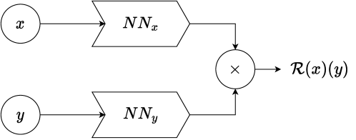
Figure 2: The DeepONet scheme.

In this work we adopt it to approximate the residual $\mathcal{R}(x)(\mu)=u(x,\mu)-u_{\text{POD}}(x,\mu)$ in a multi-fidelity approach. We can think at the mapping between the low-fidelity model (the POD/gappy POD) and the high-fidelity model as a parametric operator $\mathcal{R}(x)(\mu)$. This operator is numerically approximated by means of the DeepONet, using as dataset the low- and high-fidelity databases already computed. This architecture has demonstrated a great capability in fighting overfitting issues [44], allowing to generalize the residual even with a limited set of information.

3 Numerical results

In this section we present the numerical results obtained by applying the proposed numerical framework to a simple algebraic problem and to a Navier-Stokes problem in a 2D domain. We are going to compare the proposed method with the POD model, the gappy POD model, and with the pure deep learning approach by using DeepONet, aiming for a fair comparison with two state-of-the-art techniques for (linear and nonlinear) data-driven modeling. All the computations are performed using PyTorch [57] for the artificial neural networks, EZyRB [23] for the POD with interpolation and gappy POD calculations. To solve the Navier-Stokes equations with the finite element method we use FEniCS [43].

3.1 Algebraic parametric problem

The first test case is a simple benchmark problem inspired by [6]. The high-fidelity parametric function $f^{H}:\Omega\times P\to\mathbb{R}$ is defined as

$$f^{H}(x;\mu):=\frac{1}{2}(\mu_{1}x-2)^{2}\sin(12x-4)+\sin(\mu_{2}\cos(5x)),$$ (14)

where $x\in\Omega=[0,1]\subset\mathbb{R}$, and $\mu=(\mu_{1},\mu_{2})\in P=[2,15]\times[3,20]\subset\mathbb{R}^{2}$. The first step is to compute the function value in some points in order to build the high-fidelity database. We use different sampling strategies for the spatial and parametric domain:

• we collect $n=500$ equispaced samples $\{x_{i}^{s}\}_{i=1}^{n}$ in $\Omega$;

• we collect $36$ samples using the latin hypercube sampling, plus $4$ additional samples at the corners of the domain, for a total of $N=40$ points $\{\mu_{i}^{s}\}_{i=1}^{N}$ in $P$.

We thus compose the snapshots matrix, varying the parametric coordinates along the columns as follows:

$$\begin{bmatrix}f(x^{s}_{1},\mu^{s}_{1})&\dots&f(x^{s}_{1},\mu^{s}_{N})\\ \vdots&\ddots&\vdots\\ f(x^{s}_{n},\mu^{s}_{1})&\dots&f(x^{s}_{n},\mu^{s}_{N})\\ \end{bmatrix}\in\mathbb{R}^{n\times N}.$$ (15)

Regarding the residual learning, we use the DeepONet model structured as follows: the spatial network (branch) is composed by $2$ inner layers of $30$ neurons each, with the softplus activation function, which is the smooth version of the Rectifier Linear Unit (ReLU) [32]; the parametric network (trunk) counts $2$ inner layers with $30$ neurons and the softplus function. The output layer has $30$ neurons for both networks, without applying any additional function at this layer. The learning rate is equal to $0.005$, the $L^{2}-$regularization factor is $0.0001$.

We propose a comparison between the MF approach, POD, and DeepONet in terms of accuracy on test parameters with a fixed input database of solutions. We use different POD spaces in the comparison by selecting an increasing energetic threshold for the modes selection, aiming to analyze the difference in the error by varying the accuracy of the original POD model before getting improved by MFDeepONet. We emphasize that no preprocessing or data centering is performed on the snapshots matrix, resulting in the first mode representing a large amount of energy. This corresponds to the minimal tolerance ($0.99$) in the experiments below. Regarding the DeepONet architecture, we employ the one described above also to learn the target function without the MF setting, such that the network learns the actual unknown field instead of the residual. In this way, we want to investigate the benefit of using the two methodologies (POD and DeepONet) in a multi-fidelity fashion instead of only separately. We measure the relative error on an equispaced grid of $20\times 20$ parametric points.

POD with energy threshold 0.99.

For the POD model, we select an energy threshold $\epsilon=$0.99$$ corresponding to $N=1$ mode and radial basis function (RBF) interpolation to approximate the map between the parameters and the latent variables. The training for DeepONet and MFDeepONet lasts $10\,000$ epochs. Figure 3 shows a quantitative comparison of the three investigated techniques, presenting the relative error in the whole parametric domain, the high-fidelity samples, and the error distribution. The last plot (bottom right corner) graphically shows the technique which best performs in all the tested parameters.

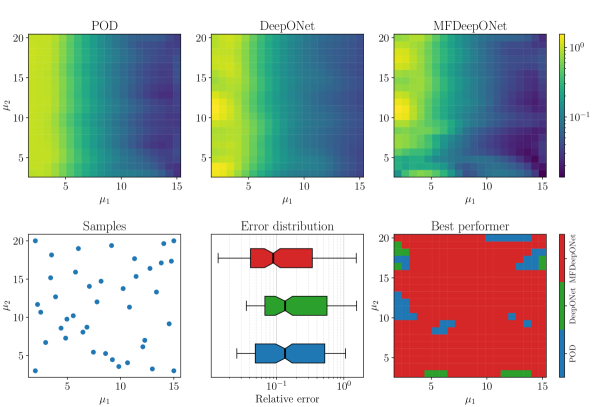
Figure 3: Comparison between POD ($0.99$ energy threshold), DeepONet, and multi-fidelity DeepONet. From top to bottom, we have the relative error in the parametric domain, the location of the high-fidelity samples in the parametric domain, the relative error distribution, and the best performers.

In this experiment, the proposed methodology outperforms both POD and DeepONet. The relative error distribution suggests that mixing the techniques helps in terms of accuracy. Indeed, even if the error shows a greater variance, the MFDeepONet is able on average to achieve the best precision among the tested methods, resulting the better approach in almost all the parametric domain. We can also note that a direct correlation between the samples location and the error distribution is not visible, confirming the DeepONet capabilities in terms of generalization and making the proposed framework effective also during the testing phase.

POD with energy threshold 0.999.

In this experiment, we replicate the previous settings with the exception of the new energy threshold for POD modes and a higher number of epochs for the machine learning models (DeepONet and MFDeepONet). Here we increase it to $\epsilon=$0.999$$ ($N=6$ modes), addressing a more accurate original model, and balancing it with longer training.

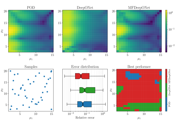
Figure 4: Comparison between POD ($0.999$ energy threshold), DeepONet, and multi-fidelity DeepONet. From top to bottom, we have the relative error in the parametric domain, the location of the high-fidelity samples in the parametric domain, the relative error distribution, and the best performers.

Figure 4 illustrates the error obtained after a $20\,000$ epochs training. The results of the previous experiments are confirmed, even if with a lower overall benefit. The error distribution in the parametric space illustrates again how the MF enhancement combines the original methods: the regions of the parametric space where the methods work better are merged using MFDeepONet, resulting in a globally more accurate model. However, using a more precise POD model (as low-fidelity) reduces the benefits of the MF approach, even with the higher number of epochs.

Gappy POD.

Here we propose the same experiments as before, this time in a sensor data scenario. Here we use $5$ sensor locations and a rank truncation equal to $10$. The involved neural networks are trained in this case for $50\,000$ epochs.

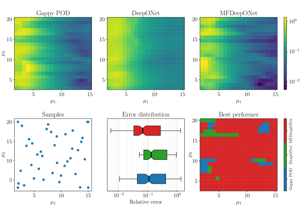
Figure 5: Comparison between gappy POD, DeepONet, and multi-fidelity DeepONet. From top to bottom, we have the relative error in the parametric domain, the location of the high-fidelity samples in the parametric domain, the relative error distribution, and the best performers.

Figure 5 summarizes the accuracy of the three tested methods, which are gappy POD, DeepONet, and MFDeepONet. The error distribution demonstrates that the multi-fidelity approach performs statistically better than the other methods. Looking at the competition between the techniques, we can also note that the multi-fidelity approach reaches the best accuracy in almost the whole parametric domain, even if at the boundaries there is a precision decrease. Such an issue could be mitigated by exploiting a better sampling strategy for the high-fidelity data.

The plots in Figure 6 provide the comparison in the spatial domain at four test parameters. The statistical results are confirmed in these examples, with the multi-fidelity approach that is able to predict most of the oscillations that the target function exhibits, contrarily to the single-fidelity approaches.

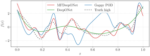
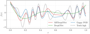
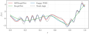
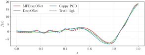
Figure 6: Examples of prediction using gappy POD, DeepONet and multi-fidelity DeepONet at different test parameters. Top left: $\mu=[4,8]$. Top right: $\mu=[3,16]$. Bottom left: $\mu=[5,18]$. Bottom right: $\mu=[8,11]$.

3.2 Navier Stokes problem

In the second numerical experiment, we test the accuracy of the proposed method for solving a parametric nonlinear PDE: the incompressible Navier-Stokes equation on a 2D domain. The numerical setting is inspired by [5].

Figure 7: Domain description.

We define the parametric vector field $u:\Omega\times P\to\mathbb{R}^{2}$ and the parametric scalar field $p:\Omega\times P\to\mathbb{R}$ such that:

$$\left\{\begin{array}[]{rll}\nu\Delta\mathbf{u}+(\mathbf{u}\cdot\nabla)\mathbf{u}+\nabla p&=0&\text{in}\,\Omega,\\ \nabla\cdot\mathbf{u}&=0&\text{in}\,\Omega,\\ \mathbf{u}&=\mu\bigl{\{}\frac{1}{2.25}(x_{1}-2)(5-x_{1}),0\bigr{\}}&\text{on}\,\Gamma_{\text{in}},\\ \mathbf{u}&=0&\text{on}\,\Gamma_{\text{wall}},\\ \nu\frac{\partial\mathbf{u}}{\partial\mathbf{n}}-p\mathbf{n}&=0&\text{on}\,\Gamma_{\text{out}},\\ \end{array}\right.$$ (16)

where $x=(x_{0},x_{1})\in\Omega\subset\mathbb{R}^{2}$ and $\mu\in P=[1,80]$. The L-shape spatial domain $\Omega$, together with the boundaries, is sketched in Figure 7. For this test case, the parametric solution is computed numerically by means of finite element discretization. The spatial domain has been tessellated into $1639$ non-overlapping elements, and for stability we apply the Taylor-Hood $P2-P1$ scheme. The high-fidelity dataset is composed of $20$ equispaced parametric samples in $P$, arranged in the snapshots matrix $U\in\mathbb{R}^{n\times N}$ with $N=20$ and $n=1639$.

The DeepONet structure for this problem is the following:

• the spatial network (branch) is composed by $3$ hidden layers of $50$ neurons each;

• the parameter network (trunk) is composed by $3$ hidden layers of $20$ neurons each.

Also in this case, the last layer of the networks has the same number of neurons, $20$. The activation function used in all the hidden layers is the Parametric ReLU (PReLU) [36], with the learning rate equal to $0.003$ and the $L^{2}-$regularization factor equal to $0.001$. The learning phase lasted $2.5\times 10^{4}$ epochs. The accuracy of the MF approach is compared to the gappy POD and to the standard DeepONet, with the same architecture (single-fidelity). The relative error is evaluated over $500$ testing points, randomly sampled in the parametric space.

POD with energy threshold 0.99.

As before, we start with a relatively poor POD model, using $N=1$ mode selected by the energetic criterion. RBF is employed also here to approximate the solution manifold at the reduced level. The number of epochs is fixed at $10\,000$ for the deep learning training.

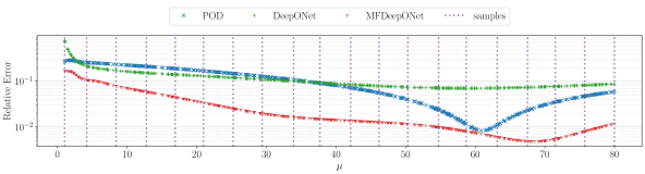
Figure 8: Comparison between POD (0.99 energy threshold), DeepONet, and multi-fidelity DeepONet in terms of relative error in the parametric domain. The vertical dotted lines indicate the location of the high-fidelity samples.

Figure 8 shows the plot of the mean relative error over the spatial domain for all the test parameters, reporting also the location of the samples in the parameter space. As for the previous experiment, the proposed technique is able to keep a higher precision in the entire domain, without showing a visible correlation between the location of the high-fidelity data and the error trend, demonstrating its robustness in terms of possible overfitting. Employing the DeepONet architecture to learn the residual (between the POD and high-fidelity models) rather than the target function results in a more efficient learning procedure, capable to ourperform the single-fidelity approaches in the entire parametric space here considered.

POD with energy threshold 0.999.

As for the previous test case, we repeat the same experiment with a more accurate POD model. Here we use $N=3$, raising the training time to $20\,000$ epochs.

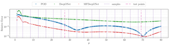
Figure 9: Comparison between POD (0.999 energy threshold), DeepONet, and multi-fidelity DeepONet in terms of relative error in the parametric domain. The vertical dotted lines indicate the location of the high-fidelity samples. The $2$ dashed vertical lines indicate the test parameters represented in Figures 10 and 11.

The trend showed in the previous investigations is confirmed, as depicted in Figure 9. The MFDeepONet method is able to produce a more accurate prediction in all the testing points, with no visible correlation with the training data. For a fair comparison, we also investigated the predicted field in the only point of the parametric domain where the MFDeepONet shows a slightly higher error with respect to the POD model (whereas the standard DeepONet performs poorly there).

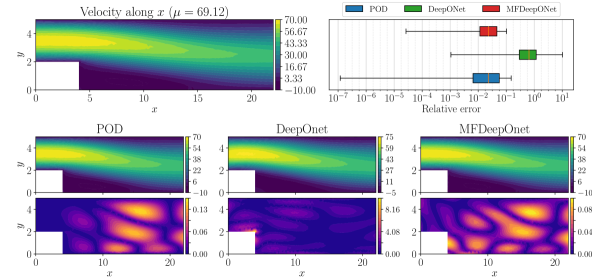
Figure 10: Representation over the spatial domain of the velocity (along $x$) in the Navier-Stokes testcase for $\mu=69.12$. The approximation computed by POD (0.999 energy threshold), DeepONet, and multi-fidelity DeepONet is shown at the bottom together with the relative error. The distribution of the error is summarized in the box plot.

Figure 10 shows the $x$-component of the velocity field for the parameter $\mu=69.12$ obtained by the three methods, with a statistical summary of the relative error. The MF approach shows here a smaller spatial variance, even if on average performs equally to the POD model. Looking instead at a different parametric coordinate (Figure 11), the benefits of the proposed approach become clear. The considerations regarding the variance of the error are still valid, but the solution for $\mu=39.95$ shows a remarkable improvement in the accuracy over the testing points.

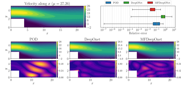
Figure 11: Representation over the spatial domain of the velocity (along $x$) in the Navier-Stokes testcase for $\mu=39.95$. The approximation computed by POD (0.999 energy threshold), DeepONet, and multi-fidelity DeepONet is shown at the bottom together with the relative error. The distribution of the error is summarized in the box plot.

Gappy POD.

The last numerical experiment focuses on the Navier-Stokes model, for which sensor data are used by the gappy POD for the low-fidelity approximation. Here we use $7$ sensor locations and a rank truncation equal to $8$. We trained the DeepONet and the MFDeepONet for $50\,000$ epochs.

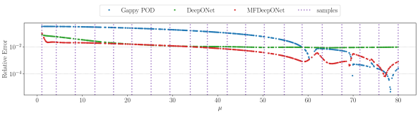
Figure 12: Comparison between gappy POD, DeepONet, and multi-fidelity DeepONet in terms of relative error in the parametric domain. The vertical dotted lines indicate the location of the high-fidelity samples.

Figure 12 reports the relative test error measured in all the test points. In this case, the standard DeepONet, is able to outperform the POD model in a large region of the parametric domain, with a relative error that remains close to $0.01$. Gappy POD is able to reach the best precision in a few test points, but also here the MF approach is the best compromise in terms of global accuracy, even if it is actually less precise than the POD model for high parameter values ($\mu>70$).

3.3 Summary discussion

This section is devoted to a summary discussion of the results obtained in the numerical investigations. For a fair comparison, we computed the mean relative test error for each method, reporting the accuracy for different neural networks training times. In addition to the previous tests, we show in Table 1 the results obtained by employing a POD space whose modes are selected with an energetic threshold of $\epsilon=$0.9999$$. The error charts for the missing cases, as well as some graphical representations of the parametric solutions, are reported in Appendix Appendix. The latter experiment aims to analyze the final accuracy when the low-fidelity POD is even more precise: the Mf approach is able to reach the best mean relative error, but its effectiveness is marginal, confirming the trend already defined in the previous tests. The combination of the POD model and DeepONet in the cascade fashion is able to reach the best accuracy in almost all the cases, but its improvement becomes marginal when the POD has good accuracy. Learning the residual however does not seem to affect the final outcome in a pejorative way, provided that the DeepONet is trained for a proper number of epochs. This is for sure a critical issue inherited by deep learning in general: we can indeed see that a longer training step does not always ensure better accuracy, producing instead over-fitting. On the practical side, the optimal settings of the network — e.g. training epochs, number of layers, type of activation function — need to be calibrated with a trial and error procedure or using more sophisticated approaches such as grid search. This calibration is out of the scope of this investigation where we want to formalize the novel framework, but surely sensitivity analysis regarding the hyper-parameters will be explored in future works. The generalization of the DeepONet, assisted also by the $L_{2}$-regularization imposed during the optimization, is able to improve accuracy over the entire parametric space, without showing a visible correlation between the location of the high-fidelity snapshots and the relative error spatial distribution.

To conclude, we highlight that the numerical experiments demonstrate a great improvement when the original POD model lacks accuracy, resulting in a great tool to treat problems where POD is not able to capture all the fluid characteristics, due to the complexity of the mathematical model or to the limited number of high-fidelity snapshots.

Table 1: The mean relative error computed in all the experiments. In bold the best results for each row.

		POD	DeepONet			MFDeepONet
			10k	20k	50k	10k	20k	50k
testcase #1	POD rank = 0.99	0.324	0.270	0.265	0.217	0.293	0.247	0.308
	POD rank = 0.999	0.203	0.270	0.265	0.217	0.196	0.193	0.127
	POD rank = 0.9999	0.098	0.270	0.265	0.217	0.093	0.104	0.178
testcase #2	POD rank = 0.99	0.105	0.116	0.068	0.072	0.030	0.022	0.030
	POD rank = 0.999	0.033	0.116	0.068	0.072	0.025	0.023	0.009
	POD rank = 0.9999	0.011	0.116	0.068	0.072	0.011	0.009	0.009

	Gappy POD	DeepONet			MFDeepONet
		10k	20k	50k	10k	20k	50k
testcase #1	0.260	0.419	0.380	0.278	0.218	0.217	0.197
testcase #2	0.135	0.035	0.033	0.017	0.029	0.010	0.009

4 Conclusions and future perspectives

In this work, we introduced a novel approach to enhance POD-based reduced order models thanks to a residual learning procedure by DeepONet. It operates by building from a limited set of data an initial low-fidelity approximation exploiting established reduced order modeling techniques. Then it learns the difference between this low-fidelity representation and the original model through the artificial neural networks, that will be inferred to predict the solution at unseen parameters. We emphasize that such an enhancement neither needs any additional evaluation of the original model nor the knowledge of the high-fidelity model, resulting in a generic data-driven improvement at a fixed computational budget. This framework has demonstrated its effectiveness in two different testcases: a univariate parametric function and a Navier-Stokes problem on a $2$-dimensional domain, showing a higher precision in both experiments with respect to the use of single-fidelities. We highlight that in these experiments the number of considered POD modes is voluntarily kept small, simulating a POD model with poor accuracy.

The present work illustrates the pipeline for POD and gappy POD for the construction of the low-fidelity model and the DeepONet architecture for residual learning. Due to its modularity, the framework is general, admitting in principle to replace the low-fidelity models with different ones. Possible future extensions should investigate adaptive samplings and sensor placement exploiting the proposed numerical framework.

Appendix

This section presents additional plots for the POD energy threshold equal to $0.9999$ case, for the algebraic function (Figure 13) and for the parametric Navier-Stokes problem (Figures 14 and 15).

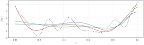
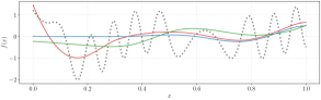
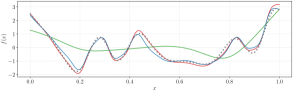
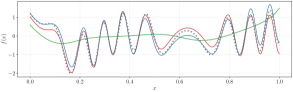
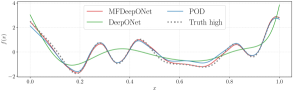
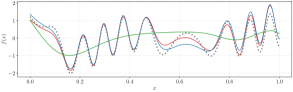
Figure 13: Predictions at two different test parameters using gappy POD, DeepONet, and multi-fidelity DeepONet with different configurations, varying the number of epochs and the POD energy threshold. The left column shows the results for $\mu=[4,8]$, while in the right one we have $\mu=[3,16]$. Top row: POD energy threshold equal to 0.99, $10000$ epochs. Center row: POD energy threshold equal to 0.999, $50000$ epochs. Bottom row: POD energy threshold equal to 0.9999, $50000$ epochs.

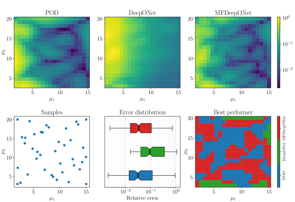
Figure 14: Comparison between POD ($0.9999$ energy threshold), DeepONet, and multi-fidelity DeepONet. From top to bottom we have the relative error in the parametric domain, the location of the high-fidelity samples in the parametric domain, the relative error distribution, and the best performers.

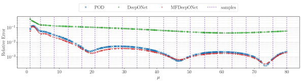
Figure 15: Comparison between POD (0.9999 energy threshold), DeepONet, and multi-fidelity DeepONet in terms of relative error in the parametric domain. The vertical dotted lines indicate the location of the high-fidelity samples.

References

- [1] R. J. Adrian. On the role of conditional averages in turbulence theory. In J. L. Zakin and G. K. Patterson, editors, Turbulence in Liquids: Proceedings of the 4th Biennial Symposium on Turbulence in Liquids, pages 323–332. University of Missouri–Rolla, 1975.
- [2] A. Alla and J. N. Kutz. Nonlinear model order reduction via dynamic mode decomposition. SIAM Journal on Scientific Computing, 39(5):B778–B796, 2017. doi:10.1137/16M105930.
- [3] D. Amsallem, M. Zahr, Y. Choi, and C. Farhat. Design optimization using hyper-reduced-order models. Structural and Multidisciplinary Optimization, 51(4):919–940, 2015. doi:10.1007/s00158-014-1183-y.
- [4] D. Amsallem, M. J. Zahr, and C. Farhat. Nonlinear model order reduction based on local reduced-order bases. International Journal for Numerical Methods in Engineering, 92(10):891–916, 2012. doi:10.1002/nme.4371.
- [5] F. Ballarin, A. Manzoni, A. Quarteroni, and G. Rozza. Supremizer stabilization of POD–Galerkin approximation of parametrized steady incompressible Navier–Stokes equations. International Journal for Numerical Methods in Engineering, 102(5):1136–1161, 2015. doi:10.1002/nme.4772.
- [6] T. Benamara, P. Breitkopf, I. Lepot, and C. Sainvitu. Multi-fidelity extension to non-intrusive proper orthogonal decomposition based surrogates. In Proceedings of the VII European Congress on Computational Methods in Applied Sciences and Engineering (ECCOMAS Congress 2016), pages 4129–4145, 2016.
- [7] P. Benner, S. Grivet-Talocia, A. Quarteroni, G. Rozza, W. H. A. Schilders, and L. M. Silveira, editors. Volume 1: System- and Data-Driven Methods and Algorithms. De Gruyter, Berlin, Boston, 2021. doi:10.1515/9783110498967.
- [8] P. Benner, S. Grivet-Talocia, A. Quarteroni, G. Rozza, W. H. A. Schilders, and L. M. Silveira, editors. Volume 2: Snapshot-Based Methods and Algorithms. De Gruyter, Berlin, Boston, 2021. doi:10.1515/9783110671490.
- [9] P. Benner, S. Grivet-Talocia, A. Quarteroni, G. Rozza, W. H. A. Schilders, and L. M. Silveira, editors. Volume 3: Applications. De Gruyter, Berlin, Boston, 2021. doi:10.1515/9783110499001.
- [10] P. Benner, M. Ohlberger, A. Patera, G. Rozza, and K. Urban. Model Reduction of Parametrized Systems, volume 17 of MS&A series. Springer, 2017.
- [11] P. Benner, E. Sachs, and S. Volkwein. Model order reduction for PDE constrained optimization. Trends in PDE constrained optimization, pages 303–326, 2014.
- [12] L. Bonfiglio, P. Perdikaris, S. Brizzolara, and G. Karniadakis. Multi-fidelity optimization of super-cavitating hydrofoils. Computer Methods in Applied Mechanics and Engineering, 332:63–85, 2018. doi:10.1016/j.cma.2017.12.009.
- [13] L. Bonfiglio, P. Perdikaris, G. Vernengo, J. S. de Medeiros, and G. Karniadakis. Improving SWATH Seakeeping Performance using Multi-Fidelity Gaussian Process and Bayesian Optimization. Journal of Ship Research, 62(4):223–240, 2018. doi:10.5957/JOSR.11170069.
- [14] I. Bright, G. Lin, and J. N. Kutz. Compressive sensing based machine learning strategy for characterizing the flow around a cylinder with limited pressure measurements. Physics of Fluids, 25(12):127102, 2013. doi:10.1063/1.4836815.
- [15] S. L. Brunton and J. N. Kutz. Data-Driven Science and Engineering: Machine Learning, Dynamical Systems, and Control. Cambridge University Press, 2019.
- [16] S. L. Brunton, J. H. Tu, I. Bright, and J. N. Kutz. Compressive sensing and low-rank libraries for classification of bifurcation regimes in nonlinear dynamical systems. SIAM Journal on Applied Dynamical Systems, 13(4):1716–1732, 2014. doi:10.1137/130949282.
- [17] T. Bui-Thanh, M. Damodaran, and K. Willcox. Aerodynamic data reconstruction and inverse design using proper orthogonal decomposition. AIAA journal, 42(8):1505–1516, 2004. doi:10.2514/1.2159.
- [18] G. Carere, M. Strazzullo, F. Ballarin, G. Rozza, and R. Stevenson. A weighted POD-reduction approach for parametrized PDE-constrained optimal control problems with random inputs and applications to environmental sciences. Computers & Mathematics with Applications, 102:261–276, 2021.
- [19] F. Chinesta, A. Huerta, G. Rozza, and K. Willcox. Model reduction methods. In E. Stein, R. de Borst, and T. J. R. Hughes, editors, Encyclopedia of Computational Mechanics, Second Edition, pages 1–36. John Wiley & Sons, Ltd., 2017.
- [20] E. Cueto, F. Chinesta, and A. Huerta. Model order reduction based on proper orthogonal decomposition. Separated Representations and PGD-Based Model Reduction: Fundamentals and Applications, pages 1–26, 2014.
- [21] B. M. de Silva, K. Manohar, E. Clark, B. W. Brunton, J. N. Kutz, and S. L. Brunton. PySensors: A Python package for sparse sensor placement. Journal of Open Source Software, 6(58):2828, 2021. doi:10.21105/joss.02828.
- [22] N. Demo, M. Tezzele, A. Mola, and G. Rozza. Hull Shape Design Optimization with Parameter Space and Model Reductions, and Self-Learning Mesh Morphing. Journal of Marine Science and Engineering, 9(2):185, 2021. doi:10.3390/jmse9020185.
- [23] N. Demo, M. Tezzele, and G. Rozza. EZyRB: Easy Reduced Basis method. The Journal of Open Source Software, 3(24):661, 2018. doi:10.21105/joss.00661.
- [24] N. Demo, M. Tezzele, and G. Rozza. A non-intrusive approach for reconstruction of POD modal coefficients through active subspaces. Comptes Rendus Mécanique de l’Académie des Sciences, 347(11):873–881, November 2019. doi:10.1016/j.crme.2019.11.012.
- [25] N. Demo, M. Tezzele, and G. Rozza. A Supervised Learning Approach Involving Active Subspaces for an Efficient Genetic Algorithm in High-Dimensional Optimization Problems. SIAM Journal on Scientific Computing, 43(3):B831–B853, 2021. doi:10.1137/20M1345219.
- [26] R. Everson and L. Sirovich. Karhunen–Loève procedure for gappy data. JOSA A, 12(8):1657–1664, 1995. doi:10.1364/JOSAA.12.001657.
- [27] I.-G. Farcas, B. Peherstorfer, T. Neckel, F. Jenko, and H.-J. Bungartz. Context-aware learning of hierarchies of low-fidelity models for multi-fidelity uncertainty quantification. arXiv preprint arXiv:2211.10835, 2022.
- [28] A. I. Forrester, A. Sóbester, and A. J. Keane. Multi-fidelity optimization via surrogate modelling. Proceedings of the Royal Society A: Mathematical, Physical and Engineering Sciences, 463(2088):3251–3269, 2007. doi:10.1098/rspa.2007.1900.
- [29] M. Gadalla, M. Cianferra, M. Tezzele, G. Stabile, A. Mola, and G. Rozza. On the comparison of LES data-driven reduced order approaches for hydroacoustic analysis. Computers & Fluids, 216:104819, 2021. doi:10.1016/j.compfluid.2020.104819.
- [30] R. Geelen, S. Wright, and K. Willcox. Operator inference for non-intrusive model reduction with quadratic manifolds. Computer Methods in Applied Mechanics and Engineering, 403:115717, 2023. doi:10.1016/j.cma.2022.115717.
- [31] O. Ghattas and K. Willcox. Learning physics-based models from data: perspectives from inverse problems and model reduction. Acta Numerica, 30:445–554, 2021. doi:10.1017/S0962492921000064.
- [32] X. Glorot, A. Bordes, and Y. Bengio. Deep sparse rectifier neural networks. In Proceedings of the fourteenth international conference on artificial intelligence and statistics, pages 315–323. JMLR Workshop and Conference Proceedings, 2011.
- [33] M. Guo, A. Manzoni, M. Amendt, P. Conti, and J. S. Hesthaven. Multi-fidelity regression using artificial neural networks: Efficient approximation of parameter-dependent output quantities. Computer Methods in Applied Mechanics and Engineering, 389:114378, 2022. doi:10.1016/j.cma.2021.114378.
- [34] J. Hart and B. v. B. Waanders. Hyper-differential sensitivity analysis with respect to model discrepancy: Calibration and optimal solution updating. arXiv preprint arXiv:2210.09044, 2022.
- [35] J. Hart and B. v. B. Waanders. Hyper-differential sensitivity analysis with respect to model discrepancy: mathematics and computation. arXiv preprint arXiv:2210.09037, 2022.
- [36] K. He, X. Zhang, S. Ren, and J. Sun. Delving deep into rectifiers: Surpassing human-level performance on imagenet classification. In Proceedings of the IEEE international conference on computer vision, pages 1026–1034, 2015.
- [37] A. A. Howard, M. Perego, G. E. Karniadakis, and P. Stinis. Multifidelity deep operator networks. arXiv preprint arXiv:2204.09157, 2022.
- [38] A. Ivagnes, N. Demo, and G. Rozza. Towards a machine learning pipeline in reduced order modelling for inverse problems: neural networks for boundary parametrization, dimensionality reduction and solution manifold approximation. arXiv preprint arXiv:2210.14764, 2022.
- [39] B. Kramer and K. E. Willcox. Nonlinear model order reduction via lifting transformations and proper orthogonal decomposition. AIAA Journal, 57(6):2297–2307, 2019. doi:10.2514/1.J057791.
- [40] J. N. Kutz, S. Sargsyan, and S. L. Brunton. Leveraging sparsity and compressive sensing for reduced order modeling. In P. Benner, M. Ohlberger, A. Patera, G. Rozza, and K. Urban, editors, Model Reduction of Parametrized Systems, volume 17 of MS&A, pages 301–315. Springer, Cham, 2017. doi:10.1007/978-3-319-58786-8\_19.
- [41] G. Lin, C. Moya, and Z. Zhang. B-deeponet: An enhanced bayesian deeponet for solving noisy parametric pdes using accelerated replica exchange sgld. Journal of Computational Physics, 473:111713, 2023.
- [42] C. Little and C. Farhat. Nonlinear Projection-Based Model Order Reduction in the Presence of Adaptive Mesh Refinement. In AIAA SCITECH 2023 Forum, 2023. doi:10.2514/6.2023-2682.
- [43] A. Logg, K.-A. Mardal, and G. Wells. Automated solution of differential equations by the finite element method: The FEniCS book, volume 84. Springer Science & Business Media, 2012.
- [44] L. Lu, P. Jin, G. Pang, Z. Zhang, and G. E. Karniadakis. Learning nonlinear operators via deeponet based on the universal approximation theorem of operators. Nature Machine Intelligence, 3(3):218–229, 2021.
- [45] L. Lu, R. Pestourie, S. G. Johnson, and G. Romano. Multifidelity deep neural operators for efficient learning of partial differential equations with application to fast inverse design of nanoscale heat transport. arXiv preprint arXiv:2204.06684, 2022.
- [46] L. Mainini and K. Willcox. Surrogate modeling approach to support real-time structural assessment and decision making. AIAA Journal, 53(6):1612–1626, 2015. doi:10.2514/1.J053464.
- [47] K. Manohar, B. W. Brunton, J. N. Kutz, and S. L. Brunton. Data-driven sparse sensor placement for reconstruction: Demonstrating the benefits of exploiting known patterns. IEEE Control Systems Magazine, 38(3):63–86, 2018. doi:10.1109/MCS.2018.2810460.
- [48] A. Manzoni, F. Negri, and A. Quarteroni. Dimensionality reduction of parameter-dependent problems through proper orthogonal decomposition. Annals of Mathematical Sciences and Applications, 1(2):341–377, 2016.
- [49] L. Meneghetti, N. Shah, M. Girfoglio, N. Demo, M. Tezzele, A. Lario, G. Stabile, and G. Rozza. A Deep Learning Approach to Improving Reduced Order Models. In G. Rozza, G. Stabile, and F. Ballarin, editors, Advanced Reduced Order Methods and Applications in Computational Fluid Dynamics, CS&E Series, chapter 20. SIAM Press, 2022. doi:10.1137/1.9781611977257.ch20.
- [50] X. Meng, H. Babaee, and G. E. Karniadakis. Multi-fidelity Bayesian neural networks: Algorithms and applications. Journal of Computational Physics, 438:110361, 2021. doi:10.1016/j.jcp.2021.110361.
- [51] X. Meng and G. E. Karniadakis. A composite neural network that learns from multi-fidelity data: Application to function approximation and inverse PDE problems. Journal of Computational Physics, 401:109020, 2020. doi:10.1016/j.jcp.2019.109020.
- [52] U. E. Morelli, P. Barral, P. Quintela, G. Rozza, and G. Stabile. A numerical approach for heat flux estimation in thin slabs continuous casting molds using data assimilation. International Journal for Numerical Methods in Engineering, 122(17):4541–4574, 2021.
- [53] N. J. Nair and A. Goza. Leveraging reduced-order models for state estimation using deep learning. Journal of Fluid Mechanics, 897, 2020. doi:10.1017/jfm.2020.409.
- [54] L. W. Ng and K. E. Willcox. Multifidelity approaches for optimization under uncertainty. International Journal for numerical methods in Engineering, 100(10):746–772, 2014. doi:10.1002/nme.4761.
- [55] S. E. Otto and C. W. Rowley. Inadequacy of linear methods for minimal sensor placement and feature selection in nonlinear systems: A new approach using secants. Journal of Nonlinear Science, 32(5):1–51, 2022. doi:10.1007/s00332-022-09806-9.
- [56] D. Papapicco, N. Demo, M. Girfoglio, G. Stabile, and G. Rozza. The neural network shifted-proper orthogonal decomposition: A machine learning approach for non-linear reduction of hyperbolic equations. Computer Methods in Applied Mechanics and Engineering, 392:114687, 2022. doi:10.1016/j.cma.2022.114687.
- [57] A. Paszke, S. Gross, F. Massa, A. Lerer, J. Bradbury, G. Chanan, T. Killeen, Z. Lin, N. Gimelshein, L. Antiga, A. Desmaison, A. Kopf, E. Yang, Z. DeVito, M. Raison, A. Tejani, S. Chilamkurthy, B. Steiner, L. Fang, J. Bai, and S. Chintala. PyTorch: An Imperative Style, High-Performance Deep Learning Library. In Advances in Neural Information Processing Systems 32, pages 8024–8035. Curran Associates, Inc., 2019.
- [58] B. Peherstorfer, K. E. Willcox, and M. Gunzburger. Survey of multifidelity methods in uncertainty propagation, inference, and optimization. SIAM Review, 60(3):550–591, 2018. doi:10.1137/16M1082469.
- [59] P. Perdikaris, M. Raissi, A. Damianou, N. D. Lawrence, and G. E. Karniadakis. Nonlinear information fusion algorithms for data-efficient multi-fidelity modelling. Proceedings of the Royal Society A, 473(2198):20160751, 2017. doi:10.1098/rspa.2016.0751.
- [60] F. Pichi, M. Strazzullo, F. Ballarin, and G. Rozza. Finite Element-Based Reduced Basis Method in Computational Fluid Dynamics. In G. Rozza, G. Stabile, and F. Ballarin, editors, Advanced Reduced Order Methods and Applications in Computational Fluid Dynamics, CS&E Series, chapter 2, pages 13–58. SIAM Press, 2022. doi:10.1137/1.9781611977257.ch2.
- [61] E. Qian, B. Kramer, B. Peherstorfer, and K. Willcox. Lift & learn: Physics-informed machine learning for large-scale nonlinear dynamical systems. Physica D: Nonlinear Phenomena, 406:132401, 2020. doi:10.1016/j.physd.2020.132401.
- [62] M. Raissi, P. Perdikaris, and G. E. Karniadakis. Inferring solutions of differential equations using noisy multi-fidelity data. Journal of Computational Physics, 335:736–746, 2017. doi:10.1016/j.jcp.2017.01.060.
- [63] J. Reiss, P. Schulze, J. Sesterhenn, and V. Mehrmann. The shifted proper orthogonal decomposition: A mode decomposition for multiple transport phenomena. SIAM Journal on Scientific Computing, 40(3):A1322–A1344, 2018.
- [64] F. Romor, M. Tezzele, M. Mrosek, C. Othmer, and G. Rozza. Multi-fidelity data fusion through parameter space reduction with applications to automotive engineering. International Journal for Numerical Methods in Engineering, 124(23):5293–5311, 2023. doi:10.1002/nme.7349.
- [65] G. Rozza, G. Stabile, and F. Ballarin. Advanced Reduced Order Methods and Applications in Computational Fluid Dynamics. Society for Industrial and Applied Mathematics, Philadelphia, PA, 2022. doi:10.1137/1.9781611977257.
- [66] O. San and R. Maulik. Neural network closures for nonlinear model order reduction. Advances in Computational Mathematics, 44:1717–1750, 2018. doi:10.1007/s10444-018-9590-z.
- [67] M. Tezzele, N. Demo, G. Stabile, A. Mola, and G. Rozza. Enhancing CFD predictions in shape design problems by model and parameter space reduction. Advanced Modeling and Simulation in Engineering Sciences, 7(40), 2020. doi:10.1186/s40323-020-00177-y.
- [68] M. Tezzele, N. Demo, G. Stabile, and G. Rozza. Nonintrusive Data-Driven Reduced Order Models in Computational Fluid Dynamics. In G. Rozza, G. Stabile, and F. Ballarin, editors, Advanced Reduced Order Methods and Applications in Computational Fluid Dynamics, CS&E Series, chapter 9. SIAM Press, 2022. doi:10.1137/1.9781611977257.ch9.
- [69] M. Tezzele, L. Fabris, M. Sidari, M. Sicchiero, and G. Rozza. A multi-fidelity approach coupling parameter space reduction and non-intrusive POD with application to structural optimization of passenger ship hulls. International Journal for Numerical Methods in Engineering, 124(5):1193–1210, 2023. doi:10.1002/nme.7159.
- [70] M. Tezzele, F. Salmoiraghi, A. Mola, and G. Rozza. Dimension reduction in heterogeneous parametric spaces with application to naval engineering shape design problems. Advanced Modeling and Simulation in Engineering Sciences, 5(1):25, Sep 2018. doi:10.1186/s40323-018-0118-3.
- [71] L. Venturi, F. Ballarin, and G. Rozza. A weighted POD method for elliptic PDEs with random inputs. Journal of Scientific Computing, 81(1):136–153, 2019. doi:10.1007/s10915-018-0830-7.
- [72] S. Volkwein. Proper orthogonal decomposition: Theory and reduced-order modelling. Lecture Notes, University of Konstanz, 4(4):1–29, 2013.
- [73] S. Wang, M. A. Bhouri, and P. Perdikaris. Fast PDE-constrained optimization via self-supervised operator learning. arXiv preprint arXiv:2110.13297, 2021.
- [74] Y. Wang, B. Yu, Z. Cao, W. Zou, and G. Yu. A comparative study of pod interpolation and pod projection methods for fast and accurate prediction of heat transfer problems. International Journal of Heat and Mass Transfer, 55(17-18):4827–4836, 2012. doi:10.1016/j.ijheatmasstransfer.2012.04.053.
- [75] K. Willcox. Unsteady flow sensing and estimation via the gappy proper orthogonal decomposition. Computers & fluids, 35(2):208–226, 2006. doi:10.1016/j.compfluid.2004.11.006.
- [76] X. Xie, M. Mohebujjaman, L. G. Rebholz, and T. Iliescu. Data-driven filtered reduced order modeling of fluid flows. SIAM Journal on Scientific Computing, 40(3):B834–B857, 2018. doi:10.1137/17M1145136.
- [77] B. Yildirim, C. Chryssostomidis, and G. Karniadakis. Efficient sensor placement for ocean measurements using low-dimensional concepts. Ocean Modelling, 27(3-4):160–173, 2009. doi:10.1016/j.ocemod.2009.01.001.
- [78] M. J. Zahr and C. Farhat. Progressive construction of a parametric reduced-order model for PDE-constrained optimization. International Journal for Numerical Methods in Engineering, 102(5):1111–1135, 2015. doi:10.1002/nme.4770.
- [79] X. Zhang, F. Xie, T. Ji, Z. Zhu, and Y. Zheng. Multi-fidelity deep neural network surrogate model for aerodynamic shape optimization. Computer Methods in Applied Mechanics and Engineering, 373:113485, 2021. doi:10.1016/j.cma.2020.113485.