A New Scheduler for URLLC in 5G NR IIoT Networks with Spatio-Temporal Traffic Correlations

Abstract

This paper explores the issue of enabling Ultra-Reliable Low-Latency Communications (URLLC) in view of the spatio-temporal correlations that characterize real 5th generation (5G) Industrial Internet of Things (IIoT) networks. In this context, we consider a common Standalone Non-Public Network (SNPN) architecture as promoted by the 5G Alliance for Connected Industries and Automation (5G-ACIA), and propose a new variant of the 5G NR semi-persistent scheduler (SPS) to deal with uplink traffic correlations. A benchmark solution with a “smart” scheduler (SSPS) is compared with a more realistic adaptive approach (ASPS) that requires the scheduler to estimate some unknown network parameters. We demonstrate via simulations that the 1-ms latency requirement for URLLC is fulfilled in both solutions, at the expense of some complexity introduced in the management of the traffic. Finally, we provide numerical guidelines to dimension IIoT networks as a function of the use case, the number of machines in the factory, and considering both periodic and aperiodic traffic.

I Introduction

The fourth Industrial Revolution (Industry 4.0) is driven by several 5th generation (5G) technologies such as Artificial Intelligence (AI) and robotics, and aims at improving the efficiency, security, and revenue of Industrial Internet of Things (IIoT) applications [1, 2]. For some IIoT processes, Ultra-Reliable Low-Latency Communications (URLLC) is required, i.e., network reliability up to 99.99999%, and end-to-end (E2E) latency below 1 ms [3, 4, 5].

From the network architecture point of view, the 3rd Generation Partnership Project (3GPP) introduces in Rel-16 (and future specifications) the paradigms of Standalone Non-Public Network (SNPN) and Public Network Interface Non-Public Network (PNI-NPN) to promote URLLC in IIoT scenarios [6, 7]. The 3GPP SNPN paradigm has also been explored by the 5G Alliance for Connected Industries and Automation (5G-ACIA) to recommend promising network architectures able to satisfy IIoT application requirements [8]. With regard to resource allocation, the 3GPP NR supports semi-persistent scheduler (SPS) in the uplink (UL) [9], in which the network pre-allocates radio resources, avoiding the need for the User Equipments (UEs) to receive uplink grants before transmission as in conventional grant-based scheduling. Many works have analyzed and demonstrated the potential of SPS to reduce the UL latency [10, 11, 12], also against some other contention-based solutions which prioritize latency at the expense of reliability [13, 14]. However, most of the prior art neglects the impact of the 5G protocol stack, thus considering the air latency instead of the more representative E2E latency, or introduces some assumptions in the traffic model. For example, in our previous contribution [15], we assumed that UEs in different machines generate packets simultaneously and according to pre-defined periodicity and size, thus neglecting the complexity of IIoT scenarios where different types of traffic may coexist.

To fill these gaps, in this paper we introduce a new, but more realistic, traffic model in which industrial machines and users activate and generate traffic, respectively, based on some specific temporal and spatial correlations. Based on that, we propose a new implementation of the SPS for IIoT networks based on a 5G-ACIA SNPN architecture, able to predict and exploit the temporal/spatial correlations of the traffic, and to pre-allocate resources accordingly. We consider two schemes: (1) the smart semi-persistent scheduler (SSPS) (our benchmark), in which a “smart” Next Generation NodeB (gNB) is assumed to have full knowledge of the system model; and (2) the adaptive semi-persistent scheduler (ASPS) in which the gNB implements a heuristic algorithm to estimate the system parameters for resource allocation. The performance of the proposed schemes is studied in terms of E2E latency against some baselines, as a function of the type of traffic (periodic or aperiodic), the offered traffic, the number of users, the bandwidth, and considering two IIoT use cases with different requirements. To do so, we develop a custom full-stack simulator implementing the 3GPP channel model proposed in [16], already tailored to IIoT environments [15], and model the total latency taking into account the time for the protocol and the control operations at the transmitter, data transmission and propagation, radio frequency (RF) processing at the receiver, and the delay introduced by the core network.

The rest of the paper is organized as follows. In Sec. II we describe our system model and simulator, in Sec. III we present our proposed SPS schemes for IIoT networks considering traffic correlations, in Sec. IV we introduce our system parameters and discuss the numerical results, and in Sec. V we conclude with suggestions for future research.

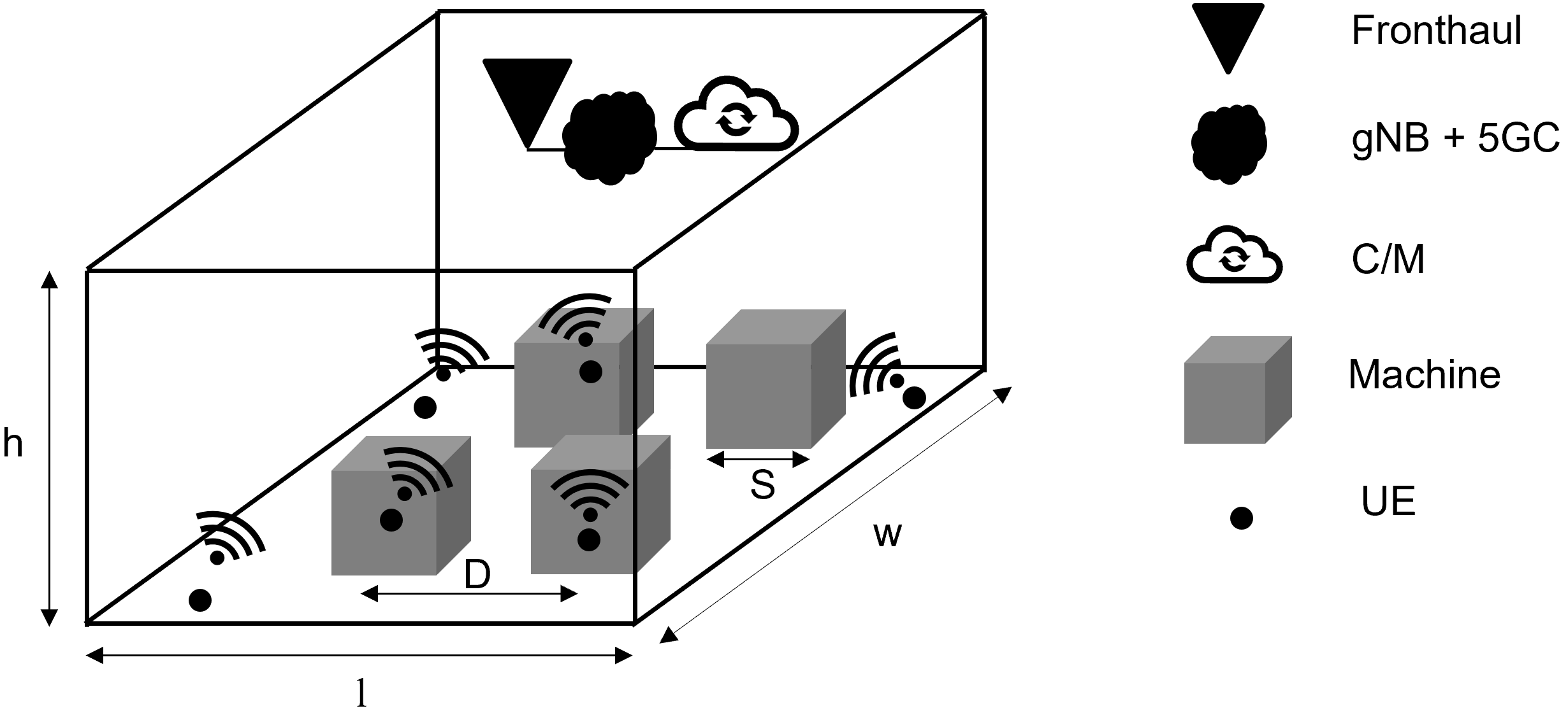
Figure 1: The baseline 5G-ACIA network architecture [8].

II End-to-End System Model

II-A Network Architecture

The reference scenario is a factory with “machines” (industrial assets in charge of different tasks), connected to an SNPN, which is a 5G remote and private network with a reserved Radio Access Network (RAN) and 5G Core (5GC). Our baseline SNPN architecture is designed according to the 5G-ACIA recommendation, as illustrated in Fig. 1, where the Controller/Master (C/M) is the IIoT central entity responsible for monitoring and controlling the machines from the 5GC.

II-B Deployment Model

The gNB and its fronthaul are located at the center of the ceiling of the factory, as shown in Fig. 1. The factory floor is modeled as a parallelepiped of length $l$, width $w$, and height $h$, as indicated in [17]. We consider $M$ machines, modeled as fixed cubes of size $S$, and deployed on the factory floor according to a uniform distribution ensuring a given inter-machine distance $D$ (evaluated from halfway across the lower base) and a minimum number of machines $M_{\rm min}$ (where both $D$ and $M_{\rm min}$ are input parameters of our simulator). Likewise, $N$ UEs are distributed following the same method, at a maximum height $S$, and can be placed onboard industrial machines, on top of walls, on metal slabs, or on robots. Inside the factory, several ”obstacles” may obstruct the communication between the UEs and the gNB.

II-C Channel Model

The channel is characterized based on the 3GPP Indoor Factory (InF) model for IIoT networks [16, Table 7.2-4] and is implemented as in our previous work  [15]. Specifically, the model suggests four InF scenarios, depending on the density of machines and the height of the UEs and of the gNB with respect to the ground. Then, the path loss depends on the condition of the channel (Line-of-Sight (LOS) or Non-Line-of-Sight (NLOS)), while the quality of the received signal is assessed in terms of the Signal-to-Noise-Ratio (SNR).

II-D Traffic Model

Unlike in previous work [15], the traffic is generated according to pre-defined IIoT-specific correlations. As such, the $M$ machines are organized in $n_{\rm lines}$ production lines, and each UE is associated with the nearest machine. When a machine in a production line activates, its UEs produce data traffic for an entire activation period of duration $\tau_{\rm on}$. The traffic model accounts for both temporal and spatial correlations. In principle, we investigate two different types of correlation:

• Inter-machine correlation, which refers to the way machines activate. When an event occurs, one machine per production line is activated. Then, machines in the same production line activate in sequence.

• Intra-machine correlation, which refers to the way UEs associated with each active machine generate data. After one machine per line is activated, the UEs associated with those machines activate too, each with probability p. Once active, each UE generates a flow of packets according to some statistics (e.g., in terms of the inter-packet interval and/or the packet size) for a whole $\tau_{\rm on}$. We consider periodic traffic, generated at constant periodicity $\tau$, or aperiodic traffic, in which the inter-data-burst interval changes according to a uniform random variable within the interval [$t_{\rm min}$, $t_{\rm max}$].

III 5G-NR Uplink Scheduler
with traffic correlations

The E2E latency is affected by the implementation of the 5G Uplink Scheduler (US), located at the gNB. After a brief overview on the baseline 5G NR SPS (Sec. III-A), in Sec. III-B we present our new SPS designs for correlated traffic.

III-A 5G NR SPS General Overview

Four messages are exchanged for the 5G NR scheduling: (1) each UE uses the Physical Uplink Control Channel (PUCCH) to ask the US for being scheduled; (2) the gNB communicates via the Physical Downlink Control Channel (PDCCH) to the UEs which resources can be used for transmission; (3) the UEs transmit their data blocks through the Physical Uplink Shared Channel (PUSCH); (4) the gNB provides the communication acknowledgment via Hybrid Automatic Repeat reQuest (HARQ). In the frequency domain, the overall bandwidth $B$ is split into $n_{\rm RB}$ Resource Blocks (RBs), each made of 12 Orthogonal Frequency Division Multiplexing (OFDM) subcarriers [18], where PUCCH, PDCCH and HARQ signals occupy one RB, whereas the number of RBs in the PUSCH depends on the modulation order, the number of mapped data blocks, and their size. On the contrary, the time domain is organized in OFDM symbols, where 7 OFDM symbols ($n_{\rm os}$) define a Scheduling Unit (SU): PUCCHs and PDCCHs occupy one SU each, while PUSCHs and HARQs form one SU, where one OFDM symbol is spent to switch from transmission to reception and vice versa under the assumption of half-duplex communication.

Every $T_{\rm IP}$, i.e., the inter-PUCCH time, each UE asks for resources by means of the PUCCH, after which the US employs one SU to process the request and allocate resources accordingly. With SPS, the US (1) estimates the times at which new data blocks will be generated until the next PUCCH opportunity; (2) allocates time/frequency resources based on the SU in which they will be served (where data blocks generated at $SU_{i}$ will be assigned to $SU_{i+1}$); and (3) notifies the UEs via the PDCCH, which takes another SU.

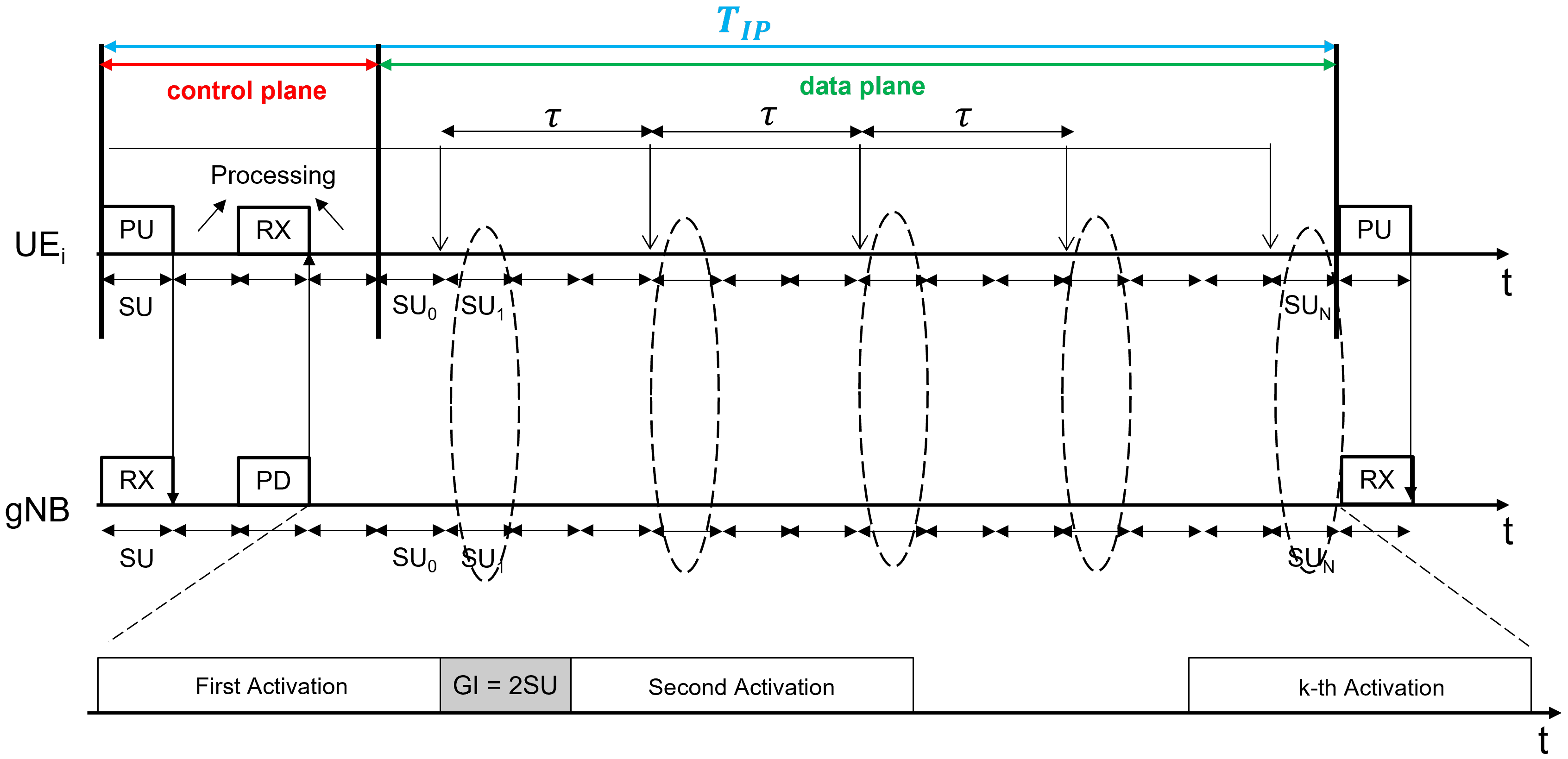
Figure 2: Timing diagram of the proposed SPS scheme for correlated traffic. The PUSCH opportunities are allocated to the $i$-th UE immediately after a new data block generation.

In our simulator, the US assigns resources according to the following criteria, in sequential order:

1. Earliest Deadline First (EDF), i.e., UEs’ requests that are closer to the 1-ms latency requirement are prioritized.

2. Fairness First (FF), i.e., UEs are served up to a given minimum level (the bucket size $B_{s}$), to promote fairness during transmission. This approach avoids that some UEs monopolize the channel at the expense of the others. If there are still resources available, the UEs’ requests beyond the bucket size are processed.

Notice that, when considering correlated traffic, at each PUCCH opportunity only a fraction of the machines in the factory is active, so only the UEs associated with those specific machines can send the PUCCH. Ideally, if the US knows the spatio-temporal statistics of the correlated traffic, it can schedule resources even without explicit scheduling requests from the UEs via the PUCCH, as we will propose to do in the following section.

III-B Proposed SPS for IIoT Correlated Traffic

In [15] we showed that SPS may be inefficient when the traffic is aperiodic, due to estimation errors in the US. In order to deal with traffic correlations, we introduce the following assumptions for aperiodic UEs.

• To avoid packet accumulation in the queue, and the possibility that packets are not transmitted on time before the UE is switched off, each UE can generate at most two packets during $\tau_{\rm on}$, as follows:

  • The first packet is generated randomly within the interval $\left[t_{\rm min},\,({t_{\rm min}+t_{\rm max}})/{2}\right]$.

  • The second packet is generated randomly within the interval [$t_{\rm min}$, $t_{\rm max}$], provided that it is within the UE’s activation period.

• The US schedules three SUs per activation period for each aperiodic UE: one SU at time $({t_{\rm min}+t_{\rm max}})/{2}$, and two SUs in the second-last and last resources of the current activation period, respectively.

• If many UEs have to send packets in the last two assigned SUs, more resources may be needed to complete their transmissions, which may involve using some of those already allocated in the following $\tau_{\rm on}$. Therefore, a guard interval (GI) of two SUs has been introduced in the data plane at the end of each activation period, to complete ongoing transmissions. The GI ensures that UEs’ transmissions in consecutive activation periods do not overlap, as depicted in Fig. 2. The effect of the GI affects the definition of $T_{\rm IP}$. In particular, we have that

  $$T_{\rm IP}=(\tau_{\rm on}+2\cdot\text{SU})\cdot n_{\rm on},$$ (1)

  where $n_{\rm on}$ is the number of activations during $T_{\rm IP}$, and is an input parameter which allows some machines to re-activate within the same $T_{\rm IP}$, especially when $M$ is small.

Based on the above assumptions, we propose two implementations of the SPS for correlated traffic.

III-B1 Smart semi-persistent scheduler (SSPS)

The “smart gNB” is fully aware of the E2E system model, including:

• the number of production lines ($n_{\rm lines}$) inside the factory;

• the number of machines ($M$) in each production line;

• both the number and the ID of the UEs associated with each machine;

• the type of traffic generated by the UEs (i.e., periodic or aperiodic), and the data block size;

• the activation period ($\tau_{\rm on}$) of the machines;

• the number of activations per $T_{\rm IP}$ ($n_{\rm on}$).

When the gNB receives the PUCCH requests from the active UEs, it can immediately identify the active machines, and those that will activate in the following $\tau_{\rm on}$. As such, the gNB can accurately predict the entire flow of activations, and schedule resources accordingly. SSPS introduces very strong assumptions at the gNB, which makes it a suitable approach for benchmarking the performance of more practical schemes.

III-B2 Adaptive semi-persistent scheduler (ASPS)

To consider a more realistic scenario, we assume that the gNB does not know a priori $\tau_{\rm on}$ and $n_{\rm on}$. Hence, the gNB implements an adaptive heuristic algorithm to estimate these missing parameters, as described in Algorithm 1. In particular, the gNB initially estimates $\hat{\tau}_{\rm on}$ and $\hat{n}_{\rm on}$ based on the values of $T_{\rm IP}$ and $n_{\rm lines}$ (known). Then, the value of $\hat{n}_{\rm on}$ is updated based on the ID of UEs sending scheduling requests in consecutive PUCCH opportunities, while the value of $\hat{\tau}_{\rm on}$ is updated based on the outcomes of previous resource allocations, that is based on the number of unused SUs in previous PUCCH opportunities.

Preliminary simulations show that a training phase of at least $3T_{\rm IP}$ is required to accurately learn $\hat{\tau}_{\rm on}$, thus to perform error-free scheduling, which has implications in terms of latency, as we will show in Sec. IV. Besides, during the training phase, some data blocks may be buffered, accumulating very long delays. For this reason, UEs adopt a dropping policy that allows queued packets to be discarded if they are not transmitted within the current activation period (GI included), thus promoting lower latency, at the cost of reduced reliability.

Algorithm 1 Adaptive semi-persistent scheduler (Sec. III-B2)

1:System Initialization

• $n_{\rm e}$: estimation cycle

• $\hat{\tau}_{\rm on}$: estimated activation period

• $\hat{n}_{\rm on}$: estimated number of activations

• $su_{\rm notx}$: list of SUs not used by UEs for data tx

• $t_{\rm notx}[i]$: instant of time corresponding to $su_{\rm notx}[i]$

• $su_{\rm tx}$: list of SUs used by UEs for data tx

• $t_{\rm tx}[i]$: instant of time corresponding to $su_{\rm tx}[i]$

2:Start

3:$n_{\rm e}=1$ $\rightarrow$ $\hat{\tau}_{\rm on}=T_{\rm IP}/{n_{\rm lines}}$ and $\hat{n}_{\rm on}={n_{\rm lines}}$

4:$n_{\rm e}=2$ $\rightarrow$ gNB recovers the activation period index ($k$) at $n_{\rm e}-1$ for UEs that sent the PUCCH at $n_{\rm e}$ $\rightarrow{\hat{n}}_{\rm on}=n_{\rm lines}+k-1$

5:Based on $\hat{n}_{\rm on}$ and $T_{\rm IP}$ $\rightarrow\hat{\tau}_{\rm on}$ even ($\hat{\tau}_{\rm on_{\rm ev}}$) or odd ($\hat{\tau}_{\rm on_{\rm od}}$)

6:gNB keeps track of $su_{\rm notx}$

7:if $\hat{\tau}_{\rm on_{\rm ev}}=\text{True}$ then

8:    $\hat{\tau}_{\rm on}=t_{\rm{\rm notx}}[0]+(n_{\rm e}-1)\,(n_{\rm os})$

9:else

10:    $\hat{\tau}_{\rm on}=t_{\rm{\rm notx}}[0]$

11:end if

12:$n_{\rm e}=3\rightarrow$ gNB keeps track of the new $su_{\rm notx}^{\rm(new)}$ and $su_{\rm tx}$

13:if $su_{\rm notx}^{\rm(new)}[0]=su_{\rm notx}[0]$ then

14:    $\hat{\tau}_{\rm on}=t_{\rm{notx}}[0]+(n_{\rm e}-1)\,(n_{\rm os})$

15:else

16:    for $i=1$ to lenght$(su_{\rm tx})$ do

17:        $\Delta=su_{\rm tx}[{i}]-su_{\rm tx}[i-1]$

18:        if $\Delta>\hat{\tau}_{\rm on}$ then

19:           $\hat{\tau}_{\rm on}^{\rm(new)}=\frac{\hat{\tau}_{\rm on}+t_{\rm tx}[i-1]}{2}$

20:           $\hat{\tau}_{\rm on}=\hat{\tau}_{\rm on}^{\rm(new)}+(n_{\rm e}-1)\,(n_{\rm os})$

21:        end if

22:    end for

23:end if

IV Performance Evaluation

In Sec. IV-C we compare the E2E latency, defined in Sec. IV-A, of different SPS schemes, based on the simulation parameters introduced in Sec. IV-B.

IV-A End-to-End Latency Analysis

In this work we evaluate the E2E latency experienced in the IIoT scenario referenced in Sec. II. The E2E latency for a single data burst (Service Data Unit (SDU) at the application layer) is computed as the time between the generation of the data burst at the UE and its reception at the C/M. Formally, the E2E latency $L$, is given by:

$$L=T_{\rm P}+T_{\rm RAN}+T_{\rm TX}+\tau_{\rm P}+T_{\rm FH}+\tau_{\rm FH}+T_{\rm gNB}+T_{\rm CN},$$ (2)

where $T_{\rm RAN}$ is the time between the generation of the data block (Packet Data Unit (PDU) at the physical layer) and its transmission over the channel, which depends on the scheduling algorithm, and on the system parameters. On the contrary, the other terms have constant values. Finally, we introduce the average E2E latency $\bar{L}$, averaged over the data blocks generated by the UEs within the simulation time $T_{S}$, and over the number of UEs.

IV-B Simulation Parameters

TABLE I: Simulation parameters.

Parameter	Description	Value
$f_{\rm c}$	Carrier frequency	3.5 GHz
$B$	Overall system bandwidth	{60,120} MHz
$\Delta f$	Subcarrier spacing	60 kHz
$SNR_{\rm th}$	SNR threshold	$-5$ dB
$T$	Noise temperature	290 K
$T_{\rm P}$	Delay to create data block	7 OFDM symbols
$T_{\rm TX}$	Data block transmission time	4 OFDM symbols
$\tau_{\rm P}$	Propagation time	0
$T_{{\rm FH}}$	Fronthaul delay	0.05 ms
$\tau_{\rm FH}$	FH-to-gNB propagation time	0
$T_{{\rm gNB}}$	gNB delay	7 OFDM symbols
$T_{\rm CN}$	5GC delay	0.1 ms
$T_{\rm S}$	Simulation time	10 s
$G_{\rm UE}=G_{\rm gNB}$	Antenna gain	0 dB
$P_{\rm TX,UL}$	UE (UL) transmit power	23 dBm
$P_{\rm TX,DL}$	gNB (DL) transmit power	30 dBm
$D$	Inter-machine distance	{5, 10} m
$S$	Side of the machines	{2, 3} m
$M_{\rm min}$	Min. number of machines	16
$l$	Length of the factory floor	{20, 50} m [8]
$w$	Width of the factory floor	{20, 10} m
$h$	Height of the factory floor	{4, 10} m
$H$	5G protocol stack header	72 bytes [19]
$B_{\rm s}$	Bucket size	40% of data burst
$p$	User activation probability	1

The simulation parameters are in Table I. We consider:

• Two use cases, defined by the 5G-ACIA: (1) augmented reality and (2) remote access and maintenance. According to the requirements in [17], and given their factory layouts, in (1) $n_{\rm lines}=4$, with four machines per line, while in (2) $n_{\rm lines}=2$, with eight machines per line.

• A subcarrier spacing of $\Delta_{f}=60$ kHz which, as observed in [15], offers lower latency compared to $\Delta_{f}=30$ kHz.

• Two values of the bandwidth, i.e., $B=$ 60 and 120 MHz, which lead to $n_{\rm RB}=$ 84 and 167 RBs, respectively.

We compare the performance of 5G NR SPS presented in Sec. III-A and deployed in [15] (referred to as baseline semi-persistent scheduler (BSPS) in the rest of the paper) with our extensions SSPS and ASPS for correlated traffic presented in Sec. III-B. Moreover, we analyze the performance of correlated traffic according to the model in Sec. II-D, for both periodic and aperiodic data, as a function of the per-user offered traffic $G$, i.e., the ratio between the data block size and the traffic periodicity.

IV-C Numerical Results

Impact of the SPS implementation. Tab. II compares the average E2E latency for BSPS, SSPS and ASPS, vs. the number of UEs $N$. We consider the augmented reality use case, $\tau_{\rm on}=$ 8 ms, $B=$ 60 MHz, and $n_{\rm on}=5$ (i.e., $T_{\rm IP}=$ 41.25 ms according to Eq. (1)). Active UEs generate periodic traffic with periodicity $\tau=2$ ms. We see that, for BSPS, $\overline{L}$ may grow indefinitely. This is due to the fact that the US can assign resources only to those UEs making scheduling requests via the PUCCH, while the others keep their data blocks in the queue, thus accumulating delays. On the other hand, SSPS and ASPS are designed to predict the spatio-temporal correlations of the traffic even without explicit PUCCH requests, and make faster scheduling decisions. While $\overline{L}\leq 1$ ms only for SSPS with $N<100$, and under the assumption that the gNB has complete information about the traffic statistics of machines and UEs, ASPS can still provide very low latency (up to $-97\%$ compared to BSPS), even though during the training phase the US may assign resources inaccurately, which implies that some data may remain in the queue and accumulate delays.

TABLE II: E2E latency vs. N, for different SPS implementations.

$N$	$\overline{L}_{\rm BSPS}$ [ms]	$\overline{L}_{\rm SSPS}$ [ms]	$\overline{L}_{\rm ASPS}$ [ms]
60	97.2	0.798	4.417
70	107.429	0.846	4.782
80	118.774	0.901	4.865
90	131.056	0.967	4.998
100	147.682	1.022	5.089

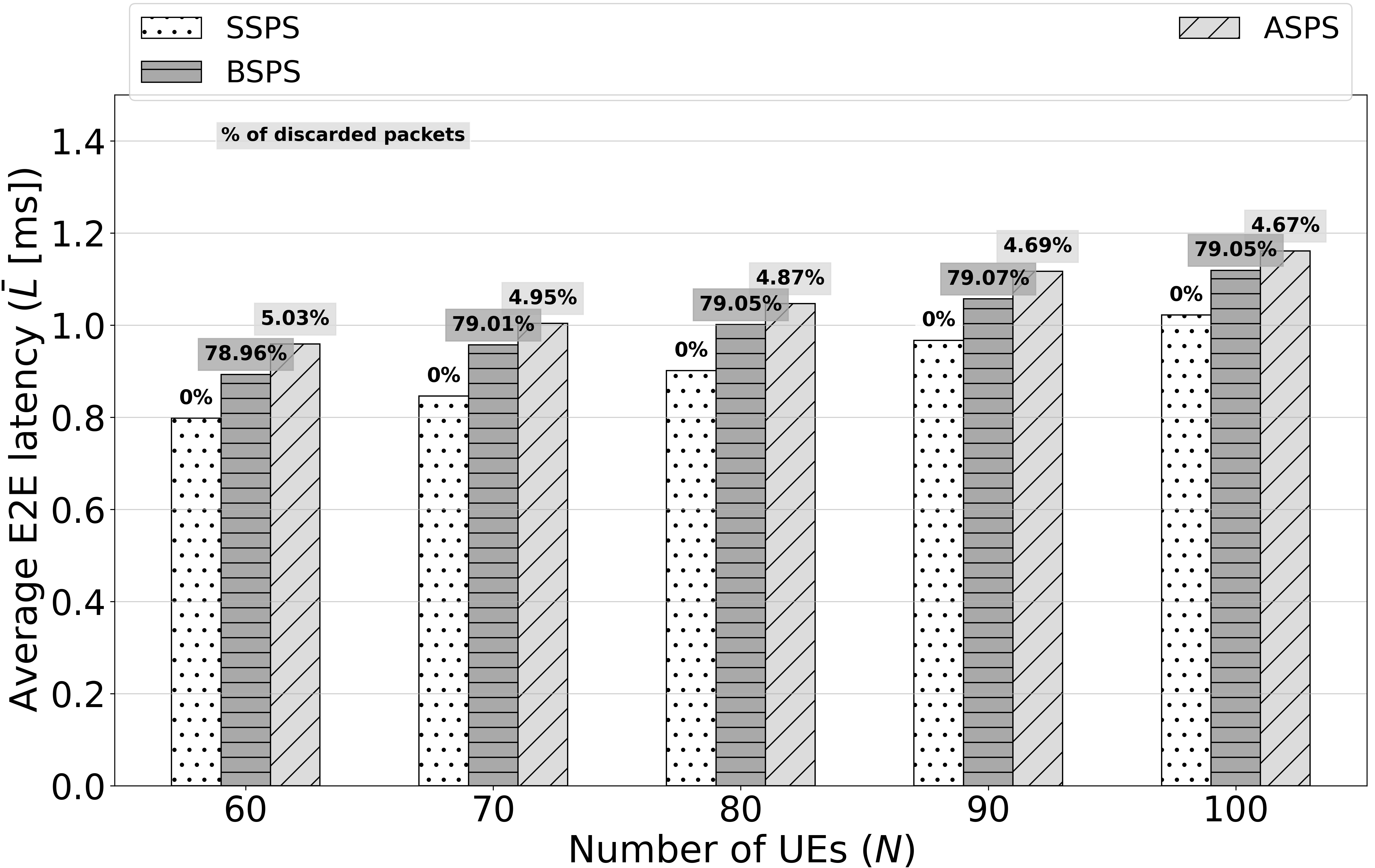
Figure 3: Average E2E latency vs. $N$, for BSPS, SSPS and ASPS with the dropping policy. We consider the augmented reality use case, $G=$ 2.75 Mbit/s, $\tau_{\rm on}=$ 8 ms, $n_{\rm on}=$ 5. Numbers on top of the bars are the packet loss ratios.

Impact of the dropping policy. In Fig. 3 we still evaluate the E2E latency for BSPS, SSPS and ASPS, but now we introduce the dropping policy as described in Sec. III-B2. While SSPS is designed to schedule resources with 100% accuracy, unscheduled packets in BSPS and ASPS will now be discarded if they are not transmitted within the UE’s activation period. The dropping policy is the result of a compromise between latency and reliability: for ASPS, we can see that $\overline{L}$ is up to 75% lower than the results in Tab. II (that do not include the dropping policy), and can satisfy the 1-ms latency requirement for URLLC as long as $N<70$, despite some packet loss. Notice that the latency for BSPS is not meaningful, as it comes with around 80% packet loss, which makes the system less congested: the (few) packets that will not be discarded because of the dropping policy are then transmitted with lower delay. As such, we can conclude that BSPS is totally unreliable for correlated traffic.

Impact of the use case and $G$. Fig. 4 shows the average E2E latency for SSPS and ASPS with the dropping policy, as a function of $G$ and of the use case. According to Eq. (1), and given that $n_{\rm on}$ is equal to the number of machines per production line, we have that for use case (1) (augmented reality) $T_{\rm IP}=33$ ms, while for use case (2) (remote access and maintenance) $T_{\rm IP}=66$ ms. As expected, the E2E latency increases with $G$ since the network is more congested. Also, the impact of the use case is remarkable: the number of machines (and, consequently, of UEs) that can be active simultaneously is proportional to $n_{\rm lines}$, and is higher for use case (1), meaning that each UE can be assigned fewer RBs on average. In these conditions, the 1-ms requirement for URLLC can always be satisfied for use case (2), while for (1) it should be $G\leq 4.25$ Mbit/s if SSPS or $G\leq 3.75$ Mbit/s if ASPS.

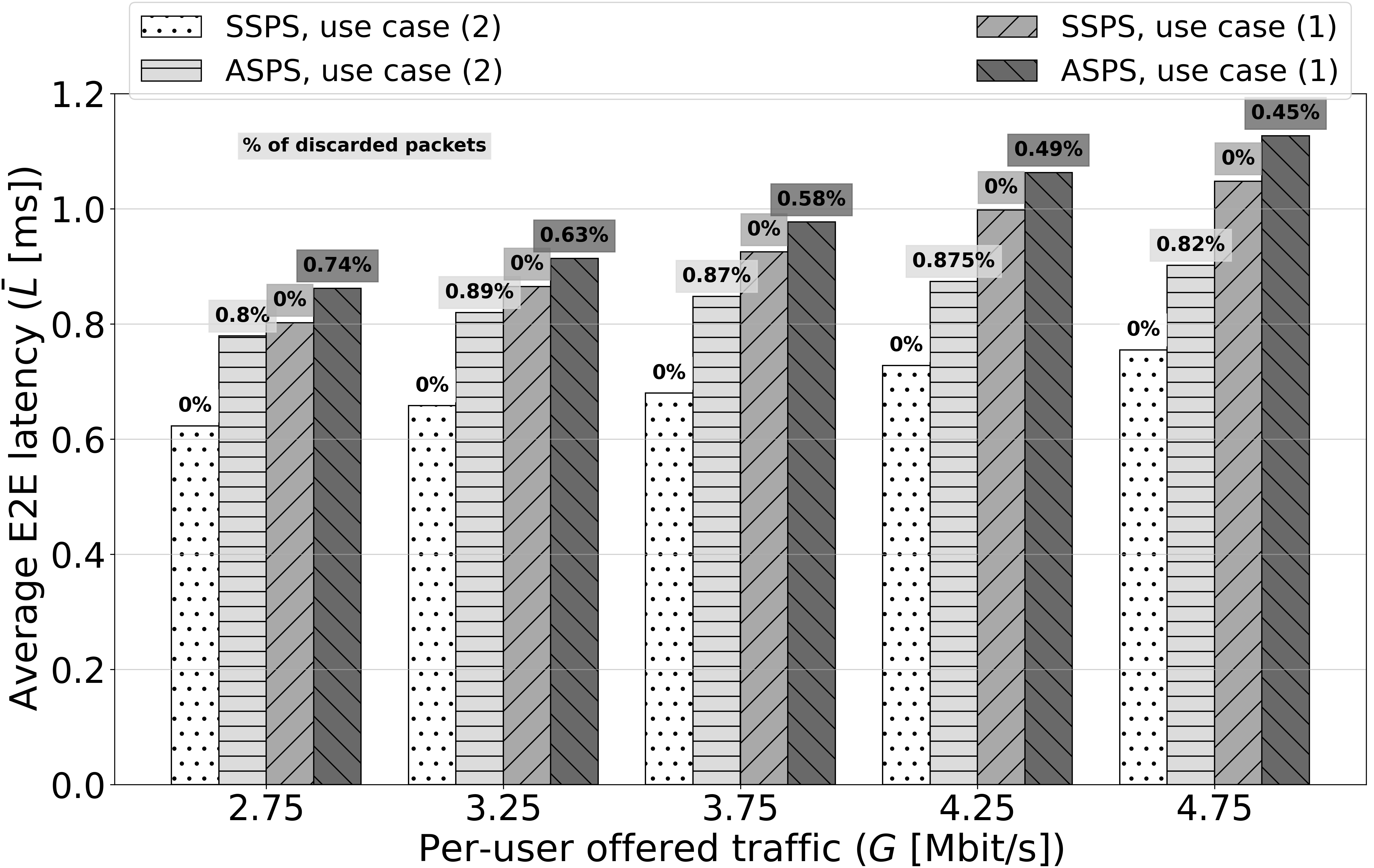
Figure 4: Average E2E latency vs. $G$ and the use case (where (1) is for augmented reality and (2) is for remote access and maintenance), for SSPS and ASPS with the dropping policy. We set $N=$ 60, $\tau_{\rm on}=$ 8 ms. Numbers on top of the bars are the packet loss ratios.

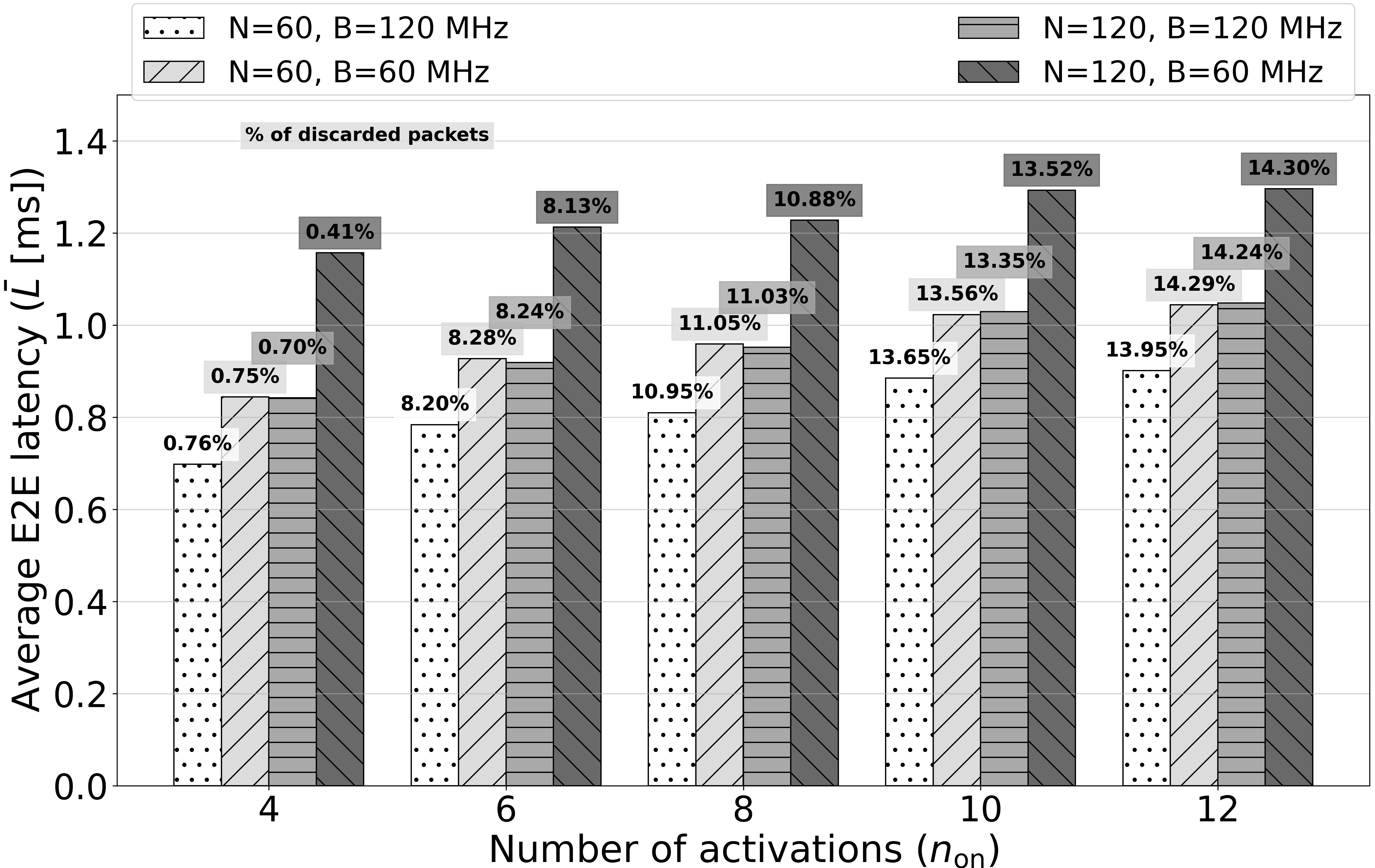
Figure 5: Average E2E latency vs. $n_{\rm on}$, $N$ and $B$ for ASPS with the dropping policy. We consider the augmented reality use case, $\tau_{\rm on}=$ 8 ms, $G=$ 2.75 Mbit/s. Numbers on top of the bars are the packet loss ratios.

Impact of the number of activations and $B$. Fig. 5 shows the average E2E latency for ASPS with the dropping policy, as a function of $n_{\rm on}$, $B$ and $N$, for the augmented reality use case and $G=$ 2.75 Mbit/s. We observe that $\overline{L}$ increases as $B$ decreases, proportionally with $N$. When $N=120$, the 1-ms URLLC latency requirement can never be achieved for $B=60$ MHz since $n_{\rm RB}$ is lower than $N$, or only when $n_{\rm on}\leq 8$ for $B=120$ MHz. When $N=60$, $\overline{L}$ is similar in both configurations, meaning that the impact of the bandwidth is negligible if the ratio between $N$ and $B$ is constant.

Moreover, $\overline{L}$ grows with the number of activations: at the beginning of the training, ASPS may underestimate $n_{\rm on}$, which implies that many data blocks would not be scheduled or, equivalently, some UEs will be assigned fewer RBs than expected, which would increase the transmission delay. Besides, the probability of underestimating ${n}_{\rm on}$ increases as the actual $n_{\rm on}$ increases, which explains the increasing trend of the packet loss in Fig. 5.

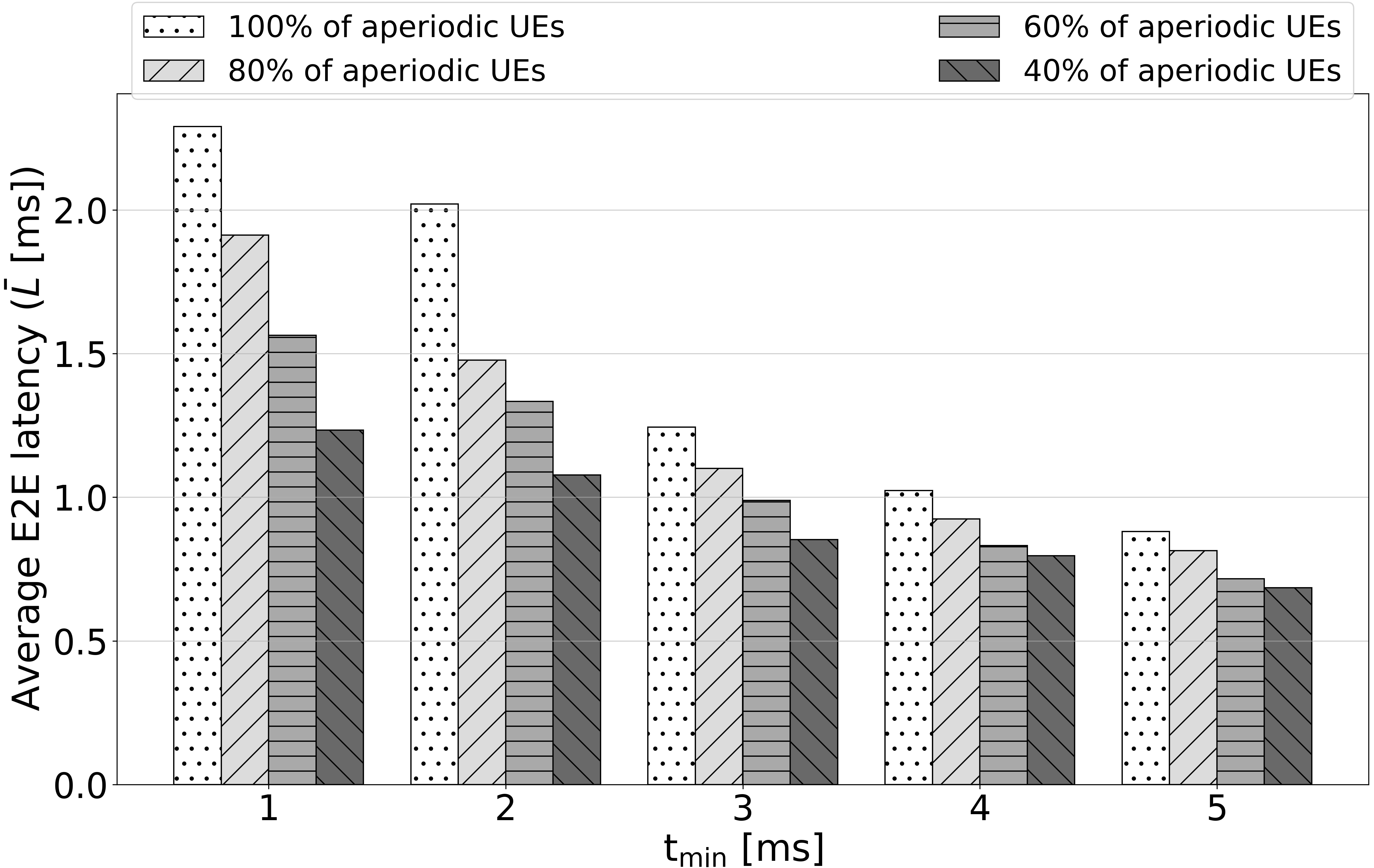
Figure 6: Average E2E latency vs. $t_{\rm min}$ and the percentage of aperiodic UEs for ASPS with the dropping policy. We set $N=$ 60, $\tau_{\rm on}=$ 8 ms, $B=$ 60 MHz, $G=$ 2.75 Mbit/s, $t_{\rm max}=$ 6 ms. Numbers on top of the bars are the packet loss ratios.

Impact of aperiodic traffic. Since the gNB has complete system information in SSPS, we explored the impact of aperiodic traffic on the E2E latency in the best case. The results are illustrated in Fig. 6 as a function of $t_{\rm min}$. We assume that $n_{\rm on}$ is equal to the number of production lines, and that {100%, 80%, 60%, 40%} of the UEs generate aperiodic traffic with $t_{\rm max}=6$ ms. We observe that $\overline{L}$ increases when $t_{\rm min}$ decreases because the traffic is more intense and the system is more congested. However, the 1-ms requirement for URLLC cannot be satisfied in most cases when introducing totally unpredictable aperiodic traffic: the requirement is met with 100% of aperiodic UEs only when $t_{\rm min}=5$ ms. This suggests that SPS (also in the best case of SSPS) is not always compatible with unpredictable traffic, even considering some degrees of correlation in the activation of machines and UEs, which motivates further studies towards more sophisticated (e.g., grant-free/distributed) scheduling methods [20].

V Conclusions

In this work we presented two new custom designs of the SPS (SSPS and ASPS, with the former that serves as a benchmark for the latter) that allocate resources in a 5G-ACIA SNPN architecture, considering IIoT-specific spatio-temporal traffic correlations. For both, we assessed the E2E latency vs. a baseline 5G NR scheduling implementation (BSPS), as a function of the bandwidth, the use case, the per-user offered traffic, and the number of UEs. Simulation results show that ASPS significantly outperforms BSPS, and can satisfy the 1-ms URLLC requirement in many configurations. However, for aperiodic traffic, no scheme can strictly support URLLC. As such, as part of our future work, we will explore the design of more advanced (learning-based) scheduling techniques to speed up the training of ASPS and achieve faster resource allocation, with considerations related to energy consumption.

VI Acknowledgment

This work has been carried out in the framework of the CNIT/WiLab-Huawei Joint Innovation Center.

It was also partially supported by the European Union under the Italian National Recovery and Resilience Plan (NRRP) of NextGenerationEU, partnership on “Telecommunications of the Future” (PE0000001 - program “RESTART”).

References

- [1] G. Aceto, V. Persico, and A. Pescapé, “A survey on information and communication technologies for industry 4.0: State-of-the-art, taxonomies, perspectives, and challenges,” IEEE Communications Surveys & Tutorials, vol. 21, no. 4, pp. 3467–3501, Fourthquarter 2019.
- [2] B. Bajic, A. Rikalovic, N. Suzic, and V. Piuri, “Industry 4.0 implementation challenges and opportunities: A managerial perspective,” IEEE Systems Journal, vol. 15, no. 1, pp. 546–559, Mar. 2021.
- [3] J. Ding, M. Nemati, C. Ranaweera, and J. Choi, “IoT Connectivity Technologies and Applications: A Survey,” IEEE Access, vol. 8, pp. 67 646–67 673, Apr. 2020.
- [4] 5G-ACIA, “5G for Industrial Internet of Things (IIoT): Capabilities, Features, and Potential,” ZVEI, November 2021.
- [5] M. Boban, M. Giordani, and M. Zorzi, “Predictive Quality of Service: The Next Frontier for Fully Autonomous Systems,” IEEE Network, vol. 35, no. 6, pp. 104–110, Nov./Dec. 2021.
- [6] 3GPP, “System architecture for the 5G System (Release 17),” Technical Report (TR) 23.501, 2021.
- [7] J. Ordonez-Lucena, J. F. Chavarria, L. M. Contreras, and A. Pastor, “The use of 5G Non-Public Networks to support Industry 4.0 scenarios,” in IEEE Conference on Standards for Communications and Networking (CSCN), 2019.
- [8] 5G-ACIA, “Integration of Industrial Ethernet Networks with 5G networks,” ZVEI, November 2019.
- [9] 3GPP, “NR; Medium Access Control (MAC) protocol specification (Release 15),” Technical Specification (TS) 38.321, 2019.
- [10] Y. Feng, A. Nirmalathas, and E. Wong, “A predictive semi-persistent scheduling scheme for low-latency applications in LTE and NR networks,” in IEEE International Conference on Communication (ICC), 2019.
- [11] Z. Arnjad, A. Sikora, B. Hilt, and J.-P. Lauffenburger, “Latency Reduction for Narrowband LTE with Semi-Persistent Scheduling,” in 4th International Symposium on Wireless Systems within the International Conferences on Intelligent Data Acquisition and Advanced Computing Systems (IDAACS-SWS), 2018.
- [12] A. Shahsin, A. Belogaev, A. Krasilov, and E. Khorov, “Adaptive Transmission Parameters Selection Algorithm for URLLC Traffic in Uplink,” in International Conference Engineering and Telecommunication (En&T), 2020.
- [13] T. Jacobsen, R. Abreu et al., “System level analysis of uplink grant-free transmission for URLLC,” in IEEE Global Communications Conference Workshops (GLOBECOM WKSHPS), 2017.
- [14] M. C. Lucas-Estañ, J. Gozalvez, and M. Sepulcre, “On the capacity of 5G NR grant-free scheduling with shared radio resources to support ultra-reliable and low-latency communications,” Sensors, vol. 19, no. 16, p. 3575, Aug. 2019.
- [15] G. Cuozzo, S. Cavallero, F. Pase, M. Giordani, J. Eichinger, C. Buratti, R. Verdone, and M. Zorzi, “Enabling URLLC in 5G NR IIoT Networks: A Full-Stack End-to-End Analysis,” in Joint European Conference on Networks and Communications & 6G Summit (EuCNC/6G Summit), 2022.
- [16] 3GPP, “Study on channel model for frequencies from 0.5 to 100 GHz (Release 16),” Technical Specification (TS) 38.901, 2019.
- [17] 5G-Clarity, “Use Case Specifications and Requirements,” ZVEI, March 2020.
- [18] E. Dahlman, S. Parkvall, and J. Skold, 5G NR: The Next Generation Wireless Access Technology. Elsevier Science, 2020.
- [19] ETSI, “Study on 5G NR User Equipment (UE) application layer data throughput performance,” Technical Report (TR) 137 901-5, 2020.
- [20] F. Pase, M. Giordani, G.Cuozzo, S.Cavallero, J. Eichinger, R. Verdone, and M. Zorzi, “Distributed Resource Allocation for URLLC in IIoT Scenarios: A Multi-Armed Bandit Approach,” IEEE Global Communications Conference Workshops (GLOBECOM WKSHPS), 2022.