pageheadfoot pagenumber chapterprefix partprefix

National Technical University of Athens

School of Electrical and Computer Engineering

Division of Computer Science

Arithmetic Approximation Techniques

& Embedded Computing Methodologies

for DSP Acceleration

Vasileios K. Leon

October 2022

Arithmetic Approximation Techniques & Embedded Computing Methodologies for Digital Signal Processing Acceleration

Vasileios Leon

Examination Committee Prof. Kiamal Pekmestzi (Supervisor), National Technical University of Athens Prof. Dimitrios Soudris, National Technical University of Athens Assoc. Prof. Georgios Goumas, National Technical University of Athens Prof. Dionysios Reisis, National and Kapodistrian University of Athens Prof. Apostolos Dollas, Technical University of Crete Prof. Dimitris Gizopoulos, National and Kapodistrian University of Athens Prof. Antonis Paschalis, National and Kapodistrian University of Athens

Submitted to National Technical University of Athens in partial fulfillment of the requirements for the degree of Doctor of Engineering (PhD in Engineering) in Computer Science.

a

of Vasileios Leon

Supervising Committee:	Kiamal Pekmestzi
	Dimitrios Soudris
	Georgios Goumas

Approved by the Examination Committee on October 10, 2022.

The Ph.D. Dissertation was partially supported by research activities of the European Space Agency (ESA).

All the reported information and views of the Ph.D. Dissertation lie entirely with the author and do not reflect the official opinion of the National Technical University of Athens.

Content that is reused from publications that the author has (co-)authored, namely excerpts, figures, and tables, is under copyright with the respective paper publishers (IEEE, ACM, IET, Elsevier). These publications are explicitly stated in the abstract of each Dissertation’s chapter. Content that is reused from third-party publications appears with the appropriate copyright note. Reuse of any such content by any interested party requires the publishers’ prior consent, according to the applicable copyright policies. Content that has not been published before is copyrighted jointly by the author of the Dissertation and the National Technical University of Athens.

Copying, storage, and distribution of this work, in whole or part of it, for commercial purposes is prohibited. Reproduction, storage, and distribution for non-profit purposes of educational or research nature is allowed, provided that the source of origin is mentioned and this copyright message is maintained. Questions concerning the use of this work for commercial purposes should be addressed to the author.

Copyright ©  Vasileios Leon, 2022 National Technical University of Athens All rights reserved. DOI: http://dx.doi.org/10.26240/heal.ntua.24738

Vasileios K. Leon PhD, Electrical & Computer Engineering, National Technical University of Athens Diploma, Computer Engineering & Informatics, University of Patras

Chapter 0 Abstract

The recent end of Dennard’s Scaling and the declining Moore’s Law have signified a new era for computing systems. Power efficiency has now become a critical factor for both cloud and edge computing. Concurrently, the rapid growth of compute-intensive applications from the Digital Signal Processing (DSP) and Artificial Intelligence (AI) domains challenges the resources of computing systems. As a result, the computing industry is forced to find alternative design approaches and computing platforms to sustain increased power efficiency, while providing sufficient performance. Among the examined solutions, Approximate Computing, Hardware Acceleration, and Heterogeneous Computing have gained great momentum. Approximate Computing is a novel design paradigm that exploits the inherent error resilience of DSP/AI applications to deliver gains in power, area, and/or performance by reducing the quality of the results. Hardware Acceleration refers to the execution of demanding computational tasks on specialized hardware, such as the Application-Specific Integrated Circuits (ASICs) and the Field-Programmable Gate Arrays (FPGAs), rather than general-purpose processors. Finally, Heterogeneous Computing refers to versatile processing architectures, such as the Vision Processing Units (VPUs), which integrate more than one type of processor and various memory technologies.

In this Dissertation, we introduce design solutions and methodologies, built on top of the preceding computing paradigms, for the development of energy-efficient DSP and AI accelerators. In particular, we adopt the promising paradigm of Approximate Computing and apply new approximation techniques in the design of arithmetic circuits. Based on our methodology, these arithmetic approximation techniques are then combined with hardware design techniques to implement approximate ASIC- and FPGA-based DSP and AI accelerators. Moreover, we propose methodologies for the efficient mapping of DSP/AI kernels on distinctive embedded devices, such as the new space-grade FPGAs and the heterogeneous VPUs. On the one hand, we cope with the decreased flexibility of space-grade technology and the technical challenges that arise in new FPGA tools and devices. On the other hand, we unlock the full potential of heterogeneity by surpassing the increased hardware complexity and exploiting all the diverse processors and memories.

In more detail, the proposed arithmetic approximation techniques involve bit-level optimizations, inexact operand encodings, and skipping of computations, while they are applied in both fixed- and floating-point arithmetic. To increase the design space and extract the most efficient solutions, we also conduct an extensive exploration on combinations among the approximation techniques. Furthermore, we propose a low-overhead scheme for seamlessly adjusting the approximation degree of our circuits at runtime. In comparison with state-of-the-art designs, the proposed arithmetic circuits feature a very large approximation space, i.e., a wide range of approximation configurations, which allows to maximize the resource gains for a given error constraint. Our techniques induce a mean relative error of up to $\scriptstyle\sim$$2\%$, i.e., typical error values for approximate circuits. The most prominent approximate circuits of the Dissertation form a high-resolution Pareto front in a comparative evaluation involving state-of-the-art designs of the literature, and they deliver up to $63\%$ better energy consumption. Finally, our runtime-configurable circuits exhibit a small area overhead of $\scriptstyle\sim$$3\%$ compared to the accurate design, and they provide $\scriptstyle\sim$$1.5\times$ less energy gains than their respective design-time counterparts with fixed approximation. Nevertheless, they can dynamically change the approximation degree, namely, the accuracy of the calculations, while they still attain remarkable energy gains versus the accurate circuit and state-of-the-art approximate circuits. At the accelerator level, we develop a plethora of approximate kernels for 1D/2D signal processing and Convolutional Neural Networks (CNNs). The experimental results show that we achieve small relative errors for classic DSP calculations and $0\%$–$5\%$ accuracy loss in CNNs for various arithmetic formats while providing up to $70\%$ area and energy savings.

Regarding the DSP acceleration on new space-grade FPGAs, we apply our methodology to efficiently map computer vision algorithms onto the radiation-hardened NanoXplore’s FPGAs. In the end, we achieve balanced resource utilization, which is comparable to that of well-established FPGA vendors. Moreover, the throughput is sufficient (e.g., up to $10$ FPS for feature detection on MPixel images), considering the performance requirements of vision-based space applications. In terms of Heterogeneous Computing, we accelerate custom DSP kernels, a sophisticated computer vision pipeline, and a demanding CNN with ResNet-50 backbone on Intel’s Myriad VPUs. The proposed methodology and embedded design techniques provide speedups up to $20\times$ for classic DSP on Myriad 2, while the power lies around $1$W. The CNN is accelerated on Myriad X with $2$W, achieving $\scriptstyle\sim$$8.5\times$ and $\scriptstyle\sim$$1.7\times$ better performance-per-Watt than the ARM CPU and the Jetson Nano GPU, respectively.

Keywords: Approximate Computing, Approximation Techniques, Arithmetic Circuits, Computer Arithmetic, Hardware Design, Hardware Accelerators, ASIC, FPGA, VPU, SoC, Heterogeneous Computing, Embedded Systems, Space-Grade, Digital Signal Processing, Computer Vision, Convolutional Neural Networks.

Chapter 1 Περιληψη

Το προςφατο τελος της Κλιµαϰωςης του Dennard ϰαι η φϑινουςα πορεια του Νοµου του Moore εχουν ςηµατοδοτηςει µια νεα εποχη για τα υπολογιςτιϰα ςυςτηµατα. Η ϰαταναλωςη ιςχυος αποτελει πλεον εναν ϰριςιµο παραγοντα, τοςο για το υπολογιςτιϰο νεφος οςο ϰαι για υπολογιςµους ςτην αϰρη του διϰτυου. Ταυτοχρονα, η ταχεια αναπτυξη απαιτητιϰων εφαρµογων απο τους τοµεις της Ψηφιαϰης Επεξεργαςιας Σηµατος (DSP) ϰαι της Τεχνητης Νοηµοςυνης (AI) δηµιουργει προϰληςεις ςτους πορους των υπολογιςτιϰων ςυςτηµατων. Ως αποτελεςµα, η βιοµηχανια των υπολογιςτων υιοϑετει εναλλαϰτιϰες µεϑοδους ςχεδιαςης ϰυϰλωµατων ϰαι ςυςτηµατων, ωςτε να διατηρηςει χαµηλη ϰαταναλωςη ιςχυος, παρεχοντας οµως ϰαι επαρϰη ταχυτητα. Αναµεςα ςτις λυςεις που εξεταζονται, ο Προςεγγιςτιϰος ϒπολογιςµος εϰµεταλλευεται την εγγενη ανϑεϰτιϰοτητα ςε ςφαλµατα των DSP/AI εφαρµογων ωςτε να προςφερει ϰερδη ςε πορους µειωνοντας την ποιοτητα των αποτελεςµατων. Η Επιταχυνςη ϒλιϰου αναφερεται ςτην εϰτελεςη απαιτητιϰων υπολογιςτιϰων εργαςιων ςε εξειδιϰευµενο υλιϰο, οπως τα Ολοϰληρωµενα Κυϰλωµατα Ειδιϰης Εφαρµογης (ASICs) ϰαι οι Συςτοιχιες Επιτοπια Προγραµµατιζοµενων Πυλων (FPGAs). Τελος, ο Ετερογενης ϒπολογιςµος αναφερεται ςε ευελιϰτες αρχιτεϰτονιϰες επεξεργαςιας µε πολλαπλους τυπους επεξεργαςτη ϰαι µνηµης, οπως οι Μοναδες Επεξεργαςιας Οραςης (VPUs).

Στην παρουςα Διατριβη, ειςαγουµε ςχεδιαςτιϰες λυςεις ϰαι µεϑοδολογιες βαςιςµενες ςτα προαναφερϑεντα προτυπα ςχεδιαςης, µε ςτοχο την αναπτυξη ενεργειαϰα αποδοτιϰων επιταχυντων υλιϰου. Σχετιϰα µε τον Προςεγγιςτιϰο ϒπολογιςµο, εφαρµοζουµε νεες τεχνιϰες προςεγγιςης ςτη ςχεδιαςη αριϑµητιϰων ϰυϰλωµατων. Οι τεχνιϰες αυτες ςυνδυαζονται µε βαςη τη µεϑοδολογια µας µε ϰλαςςιϰες τεχνιϰες ςχεδιαςης, ωςτε να υλοποιηςουµε προςεγγιςτιϰους DSP ϰαι AI επιταχυντες ςε ASIC ϰαι FPGA. Επιπλεον, προτεινουµε µεϑοδολογιες για την αποτελεςµατιϰη αποτυπωςη DSP/AI πυρηνων πανω ςε ιδιοµορφες ενςωµατωµενες ςυςϰευες, οπως τα νεα FPGAs διαςτηµιϰου βαϑµου ϰαι οι ετερογενεις VPUs. Οςον αφορα τα FPGAs, αντιµετωπιζουµε τις τεχνιϰες προϰληςεις που προϰυπτουν ϰατα τη χρηςη νεων εργαλειων, ενω για τις VPUs, ξεϰλειδωνουµε ολες τις δυνατοτητες της ετερογενειας, ξεπερνωντας την αυξηµενη πολυπλοϰοτητα υλιϰου ϰαι αξιοποιωντας ολους τους διαφορετιϰους πορους.

Οι προτεινοµενες τεχνιϰες αριϑµητιϰης προςεγγιςης περιλαµβανουν βελτιςτοποιηςεις ςε επιπεδο δυαδιϰου ψηφιου, µη αϰριβεις ϰωδιϰοποιηςεις τελεςτων, ϰαι παραλειψη υπολογιςµων, ενω εφαρµοζονται ςε αριϑµητιϰη τοςο ςταϑερης οςο ϰαι ϰινητης υποδιαςτολης. Για να αυξηϑει ο χωρος ςχεδιαςης ϰαι να εξαγουµε τις πιο αποτελεςµατιϰες λυςεις, πραγµατοποιουµε επιςης µια εϰτενη εξερευνηςη πανω ςτους ςυνδυαςµους των τεχνιϰων. Επιπλεον, προτεινουµε ενα ςχηµα χαµηλης επιβαρυνςης για την απροςϰοπτη ρυϑµιςη του βαϑµου προςεγγιςης των ϰυϰλωµατων ϰατα το χρονο εϰτελεςης. Σε ςυγϰριςη µε ςηµαντιϰα ϰυϰλωµατα της βιβλιογραφιας, οι προτεινοµενες λυςεις διαϑετουν πολυ µεγαλυτερο χωρο προςεγγιςης (ευρυτερο φαςµα προςεγγιςεων), επιτρεποντας τη µεγιςτοποιηςη των ϰερδων ςε πορους για εναν δεδοµενο περιοριςµο ςφαλµατος. Οι τεχνιϰες µας προϰαλουν ενα µεςο ςχετιϰο ςφαλµα εως ϰαι $\scriptstyle\sim$$2\%$, δηλαδη τυπιϰες τιµες ςφαλµατος προςεγγιςτιϰων ϰυϰλωµατων. Τα πιο εξεχοντα προςεγγιςτιϰα ϰυϰλωµατα της Διατριβης ςχηµατιζουν ενα ςυνορο Pareto υψηλης αναλυςης ςτη ςυγϰριτιϰη αξιολογηςη µε ςηµαντιϰες εργαςιες της βιβλιογραφιας, προςφεροντας εως ϰαι $63\%$ ϰαλυτερη ϰαταναλωςη ενεργειας. Τελος, τα ϰυϰλωµατα που µπορουν να ρυϑµιςουν δυναµιϰα την προςεγγιςη, εχουν αυξηµενη επιφανεια ϰατα $\scriptstyle\sim$$3\%$ ςε ςυγϰριςη µε το αϰριβες ϰυϰλωµα, ϰαι παρεχουν $\scriptstyle\sim$1.5$\times$ λιγοτερα ϰερδη ενεργειας απο τα αντιςτοιχα ϰυϰλωµατα µε ςταϑερη προςεγγιςη. Οµως, εχουν τη δυνατοτητα να αλλαζουν την αϰριβεια των υπολογιςµων, ενω εξαϰολουϑουν να προςφερουν αξιοςηµειωτα ενεργειαϰα ϰερδη εναντι του αϰριβους ϰυϰλωµατος ϰαι ϰυϰλωµατων της βιβλιογραφιας. Σε επιπεδο επιταχυντη, αναπτυςςουµε µια πληϑωρα απο προςεγγιςτιϰους πυρηνες για επεξεργαςια ςηµατων/ειϰονων ϰαι Συνελιϰτιϰα Νευρωνιϰα Διϰτυα (CNNs). Με βαςη την πειραµατιϰη αναλυςη, τα ςφαλµατα ειναι µιϰρα ςε ϰλαςιϰους DSP υπολογιςµους ϰαι η απωλεια αϰριβειας ϰυµαινεται ως $5\%$ ςτα νευρωνιϰα διϰτυα, ενω επιτυγχανεται εως ϰαι $70\%$ εξοιϰονοµηςη επιφανειας ϰαι ενεργειας.

Σχετιϰα µε τα νεα FPGAs διαςτηµιϰου βαϑµου, εφαρµοζουµε τη µεϑοδολογια µας για την αποτελεςµατιϰη απειϰονιςη αλγοριϑµων υπολογιςτιϰης οραςης ςτα ανϑεϰτιϰα-ςε-αϰτινοβολια FPGAs της NanoXplore. Στο τελος, επιτυγχανουµε ιςορροπηµενη χρηςη πορων, η οποια ειναι ςυγϰριςιµη µε αυτη των ϰαϑιερωµενων προµηϑευτων FPGAs. Επιπλεον, η ταχυτητα ειναι επαρϰης (π.χ., εως ϰαι $10$ FPS για την ανιχνευςη χαραϰτηριςτιϰων ςε MPixel ειϰονες), λαµβανοντας υποψη τις απαιτηςεις αποδοςης των διαςτηµιϰων εφαρµογων. Σχετιϰα µε τον Ετερογενη ϒπολογιςµο, επιταχυνουµε DSP πυρηνες, µια αϰολουϑια αλγοριϑµων υπολογιςτιϰης οραςης, ϰαι ενα απαιτητιϰο CNN ςτις Myriad VPUs της Intel. Οι προτεινοµενες µεϑοδολογιες ϰαι τεχνιϰες ενςωµατωµενης ςχεδιαςης παρεχουν επιταχυνςη εως ϰαι $20\times$ ςε ϰλαςιϰους DSP υπολογιςµους ςτη Myriad 2 µε ϰαταναλωςη ιςχυος $1$W. Το CNN επιταχυνεται ςτη Myriad X µε $2$W, προςφεροντας $\scriptstyle\sim$8.5$\times$ ϰαι $\scriptstyle\sim$1.7$\times$ ϰαλυτερη αποδοςη-ανα-Watt απο τον επεξεργαςτη γενιϰου-ςϰοπου ARM ϰαι τον επεξεργαςτη γραφιϰων Jetson Nano, αντιςτοιχα.

Λεξεις Κλειδια: Προςεγγιςτιϰος ϒπολογιςµος, Τεχνιϰες Προςεγγιςης, Αριϑµητιϰα Κυϰλωµατα, Αριϑµητιϰη ϒπολογιςτων, Σχεδιαςη ϒλιϰου, Επιταχυντες ϒλιϰου, Ετερογενης ϒπολογιςµος, Ενςωµατωµενα Συςτηµατα, Τεχνολογια Διαςτηµατος, Ψηφιαϰη Επεξεργαςια Σηµατος, ϒπολογιςτιϰη Οραςη, Συνελιϰτιϰα Νευρωνιϰα Διϰτυα.

Contents

1. 0 Abstract
2. 1 Greek Abstract
3. List of Abbreviations
4. 2 Introduction
   1. 1 The Landscape of Embedded Systems
   2. 2 The Evolution of Integrated Circuits
   3. 3 Approximate Computing
   4. 4 Hardware Acceleration
   5. 5 Heterogeneous Computing
   6. 6 Scope and Contribution of Dissertation
   7. 7 Structure of Dissertation
   8. 8 Overview of Technologies, Tools and Devices
5. 3 The Approximate Computing Paradigm
   1. 1 Introduction
   2. 2 The Terminology of Approximate Computing
   3. 3 Classification of Software Approximation Techniques
      1. 1 Selective Task Skipping
      2. 2 Approximate Memoization
      3. 3 Relaxed Synchronization
      4. 4 Precision Scaling
      5. 5 Data Sampling
      6. 6 Approximate Programming Languages
   4. 4 Classification of Hardware Approximation Techniques
      1. 1 Circuit Functional Approximation
      2. 2 Voltage Over-Scaling
      3. 3 Over-Clocking
6. 1 Arithmetic Approximation Techniques for Circuit Design
   1. 4 Arithmetic Optimization: Double-LSB Encoding
      1. 1 Introduction
      2. 2 The Double Least Significant Bit Format
      3. 3 Design of DLSB Multiplication Circuits
         1. 1 Straightforward DLSB Design
         2. 2 Sophisticated DLSB Design
      4. 4 Evaluation
         1. 1 Theoretical Analysis
         2. 2 Experimental Results
         3. 3 Case Study: DLSB for Large-Size Multiplication
      5. 5 Conclusion
   2. 5 Arithmetic Approximation: Hybrid High-Radix Encoding
      1. 1 Introduction
      2. 2 Design of Approximate High-Radix Encodings and Multipliers
         1. 1 Approximate Operand Encoding

List of Figures

1. 1 Number of Connected IoT Devices from 2015 to 2025
2. 2 50 Years Trends in Microprocessors
3. a
4. 5 The Structure of the Ph.D. Dissertation
5. 6 The Goal of the Ph.D. Dissertation
6. 1 Classification of State-of-the-Art Software Approximation Techniques
7. 2 Classification of State-of-the-Art Hardware Approximation Techniques
8. 1 DLSB Addition and Subtraction
9. 2 Circuits of the DLSB Multipliers
10. 2 Sophisticated DLSB Design
11. 4 Resource Gains of the DLSB Multiplier

List of Tables

1. List of Abbreviations
2. 1 Overview of Dissertation’s Tools and Devices
3. 1 Basic Terminology of Approximate Computing
4. 2 Classification of Software Approximation Techniques
5. 3 Classification of Hardware Approximation Techniques
6. 1 Modified Booth Encoding
7. 2 Components of the Conventional and DLSB Multipliers
8. 3 Unit Gate Overhead of the DLSB Multipliers
9. 4 Synthesis Results of the DLSB Multipliers on TSMC 45-nm Standard-Cell
10. 1 Accurate Radix-$4$ Encoding
11. 2 Approximate High-Radix-$2^{k}$ Encoding

List of Abbreviations

AI	Artificial Intelligence
ALU	Arithmetic Logic Unit
ANN	Artificial Neural Network
ASIC	Application-Specific Integrated Circuit
BER	Bit Error Rate
BRAVE	Big Re-programmable Array for Versatile Environments
CER	Correct Edge Ratio
CFA	Circuit Functional Approximation
CIF	Camera Interface
CKG	Clock Generator
CMB	Conventional Modified Booth
CMX	Connection Matrix
CNN	Convolutional Neural Network
CORDIC	Coordinate Rotation Digital Computer
COTS	Commercial-Off-The-Shelf
CPU	Central Processing Unit
CUDA	Compute Unified Device Architecture
CV	Computer Vision
CY	Carry Unit
DDR	Double Data Rate
DFF	Delay Flip-Flop
DLSB	Double Least Significant Bit
DMA	Direct Memory Access
DNN	Deep Neural Network
DRAM	Dynamic Random Access Memory
DSE	Design Space Exploration
DSP	Digital Signal Processing
ECR	Erroneous Classification Ratio
EDAC	Error Detection And Correction
EO	Earth Observation
ESA	European Space Agency
FE	Functional Element
FIFO	First-In First-Out
FIR	Finite Impulse Response
FPGA	Field-Programmable Gate Array
FPS	Frames Per Second
FPU	Floating-Point Unit
GPU	Graphics Processing Unit
HDL	Hardware Description Language
IoT	Internet of Things
LCD	Liquid Crystal Display
LEO	Low Earth Orbit
LLR	Log-Likelihood-Ratio
LNS	Logarithmic Number System
LOCE	Location Error
LSB	Least Significant Bit
LUT	Look-Up Table
MB	Modified Booth
MDK	Myriad Development Kit
ML	Machine Learning
MPDS	Mega Pixel Disparities per Second
MRED	Mean Relative Error Distance
MSB	Most Significant Bit
NaN	Not-a-Number
NCE	Neural Computer Engine
NCS	Neural Computer Stick
OC	Over-Clocking
ORIE	Orientation Error
PDF	Probability Density Function
PE	Processing Element
PLL	Phase-Locked Loop
PON	Possibility of Overflow-Normal
PP	Partial Product
PRED	Possibility of Relative Error Distance
PSNR	Peak Signal-to-Noise Ratio
PUN	Possibility of Underflow-Normal
QAM	Quadrature Amplitude Modulation
QoS	Quality of Service
RAMB	Random Access Memory Block
RED	Relative Error Distance
RF	Register File
RH	Radiation Hardened
RNS	Residue Number System
ROM	Read-Only Memory
RT	Radiation Tolerant
RTL	Register-Transfer Level
SHAVE	Streaming Hybrid Architecture Vector Engine
SIMD	Single Instruction Multiple Data
SIPP	Streaming Image Processing Pipeline
SNR	Signal-to-Noise Ratio
SoC	System-on-Chip
SoM	System-on-Module
SRAM	Static Random Access Memory
STA	Static Timing Analysis
SSIM	Structural Similarity Index
SWaP	Size, Weight and Power
TDP	Thermal Design Power
TMR	Triple Modular Redundancy
TOPS	Tera Operations Per Second
TPU	Tensor Processing Unit
UART	Universal Asynchronous Receiver-Transmitter
VBN	Vision-Based Navigation
VLIW	Very Long Instruction Word
VOS	Voltage Over-Scaling
VPU	Vision Processing Unit
WFG	Waveform Generator

IEEEexample:BSTcontrol

Chapter 2 Introduction

1 The Landscape of Embedded Systems

The rapid technological advancements in processing, communication, storage, and sensing have transformed the landscape of embedded systems. With the emergence of Internet of Things (IoT) [iot_elsi], there is a huge increment in the amount of data that are generated, which imposes technical challenges in the typical resource-constrained devices. On the other hand, the transmission of all these data to cloud infrastructures and data centers for processing creates communication bottlenecks, does not guarantee real-time response, while it is often avoided due to safety and privacy issues. Due to the ever-growing number of IoT connections, which is expected to be 27 billion in 2025 (as shown in Figure 1), the original cloud-centric system is already stressed to meet the runtime requirements. As a result, there is a tendency to process the data at the edge of the network, namely, upon they are generated. This new computing paradigm is established by the name Edge Computing [edge_ieee] and has gained significant momentum over the last years.

Concurrently, the massive growth of demanding applications and powerful algorithms from domains such as Digital Signal Processing (DSP), Computer Vision (CV), Artificial Intelligence (AI), and Machine Learning (ML), marks a new era for the computing systems at the edge. Conventional embedded processors, such as Central Processing Units (CPUs) and microcontrollers, do not have the computational power to handle these compute-intensive workloads, and thus, they are unable to meet the performance requirements [glent, georgis, ai_edge]. Another limitation is the restricted memory capacity at the edge, which slows down the processing, especially in applications with a large amount of I/O data.

It is evident that the proliferation of data along with the emergence of applications with increased complexity requires alternative design solutions to sustain sufficient performance at the edge. For this reason, the embedded systems have evolved over the years and constitute multi-purpose systems that sense, act, and communicate with their environment. In earlier years, the embedded systems consisted of simple microcontrollers and memories. In contrast, contemporary embedded systems are build on complex System-on-Modules (SoMs) and System-on-Chips (SoCs), i.e., they are placed in single boards and single chips, respectively. These systems integrate CPUs, novel specialized processors, memory blocks, high-bandwidth peripherals, and communication interfaces. Nevertheless, besides space limitations, there is a vital factor that does not allow to seamlessly increase the computation resources, e.g., by adding more devices and/or processing units: the power consumption. Typical embedded systems consume some Watts [embed_power], while ultra-low-power embedded systems (e.g., wearable) have a power budget of a few milliWatts [embed_power2]. Consequently, there is a trade-off between performance and power: from the one side, the applications demand speed and real-time response, while from the other side, there are tight power constrains at the edge.

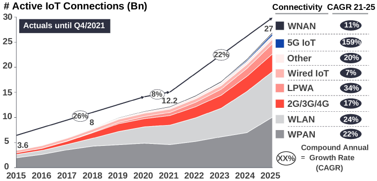
Figure 1: Number of connected IoT devices from 2015 to 2025. Source: IoT Analytics, https://iot-analytics.com/number-connected-iot-devices/.

2 The Evolution of Integrated Circuits

The integrated circuits constitute the cornerstone of computing systems, as they inherently impact their performance, power consumption, and area utilization. Figure 2 illustrates the trends for the microprocessors over the last 50 years. Historically, the semiconductor technology was driven for more than 40 years by two fundamental principles: Moore’s Law [moore] and Dennard’s Law [dennard]. According to Gordon Moore [moore], the number of transistors in a dense integrated circuit doubles approximately every two years. As shown in Figure 2, the transistor scaling is linear until today, even though several researchers forecast that Moore’s Law will end soon [moore_future]. Moore’s Law is often quoted together with the prediction of David House (executive of Intel), who then said that the overall computing performance would double approximately every 18 months. On the other hand, Dennard’s Law, which expired in the mid-2000s, is the force behind Moore’s Law. According to Robert Dennard [dennard], the power density (power per silicon area) remains stable as the transistors get smaller, so that the power use stays in proportion with the area, i.e., both voltage and current scale (downward) with the length. Practically, for a given area size, the power consumption of the chip remained the same in each transition to a new generation of process technology (technological node). Therefore, each new process technology doubled the number of transistors in a chip without increasing the power consumption. The combination of the two laws allowed to scale the supply voltage and the threshold voltage, resulting in lower power per transistor, and thus, almost stable power density.

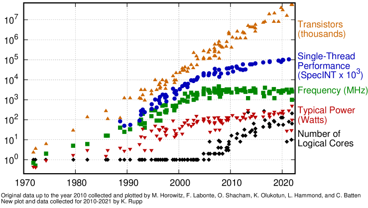
Figure 2: 50-year trends in microprocessors. Source: Karl Rupp, https://github.com/karlrupp/microprocessor-trend-data.

Nevertheless, the scaling law of Dennard did not consider the impact of the transistor sub-threshold leakage on the total chip power [dennardend7]. More specifically, in technological nodes of some nanometers, the decrease of the threshold voltage results in an exponential increase of the leakage power. This did not happen in 1970s, because the sub-threshold leakage was small and had negligible impact on the total chip power. As a result, the threshold voltage can no longer be reduced, and thus, the scaling of the supply voltage stopped (further scaling could affect the performance).

In summary, even though the number of transistors integrated per area is increasing, the supply voltage is not scaled accordingly, and thus, the power density is increased. The failure of Dennard’s scaling in conjunction with other factors such as the cooling technology and the natural limits of silicon has led us to the “Dark Silicon” era [dark1, dark2, dark3]. In this era, the entire circuitry of an integrated circuit cannot be powered-on at the nominal operating voltage for a given Thermal Design Power (TDP) constraint. All the things considered, the power efficiency and management is nowadays a critical issue for computing systems, either they are placed at the edge (embedded systems) or on the cloud (data centers). Therefore, the industry of computing systems is forced to find new design approaches and computing platforms, which will improve the power efficiency while providing the desired performance.

Towards power-efficient, real-time, and high-yielding computing systems, Approximate Computing [2013_Han_ETS, 2016_Mittal_ACMsrv, 2016_Xu_IEEEdt, Shafique_2016, 2021_Stanley_ACMsrv], Hardware Acceleration [glent, georgis, kachris, accel1, accel2], and Heterogeneous Computing [heter1, heterbook, heterog, heter2, heter3] have attracted much interest from the research community. The Approximate Computing paradigm exploits the error resilience of applications from the DSP/AI domains to reduce the quality of the results and deliver in exchange gains in power, area, and/or performance. Hardware Acceleration refers to the process of offloading compute-intensive tasks onto specialized hardware, such as the Application-Specific Integrated Circuits (ASICs) and the Field-Programmable Gate Arrays (FPGAs), rather than executing them on general-purpose CPUs. Finally, Heterogeneous Computing refers to systems integrating more than one type of processor, such as the Graphics Processing Units (GPUs) and the Vision Processing Units (VPUs). These design approaches are inherently linked and overlapping each other: (i) practically, heterogeneous hardware architectures (i.e., GPUs and VPUs) belong in the wider range of hardware accelerators, and (ii) approximations can be applied in implementations of all the hardware accelerators.

3 Approximate Computing

Approximate computations have been applied since the 1960s. For example, in one of the first works of the field, Mitchell proposed the logarithmic-based multiplication/division [1962_Mitchell]). Nevertheless, the first systematic efforts to define the Approximate Computing paradigm started in the late 2000s. Since then, various terms have been used to describe the process of generating approximate architectures, programs, and circuits. Approximate Computing is synonymous or overlaps with them. The most well-known terms of the literature are listed as follows:

• Chakradhar et al. [ChakradharDAC2010] define “Best-Effort Computing” as “the approach of designing software/hardware computing systems with reduced workload, improved parallelization and/or approximate components towards enhanced efficiency and scalability”.

• Carbin et al. [2012_Carbin_PLDI] introduce the term “Relaxed Programming” to express “the transformation of programs with approximation methods and relaxed semantics to enable greater flexibility in their execution”.

• Chippa et al. [2014_Chippa_IEEEtvlsi] use the term “Scalable Effort Design” for “the systematic approach that embodies the notion of scalable effort into the design process at different levels of abstraction, involving mechanisms to vary the computational effort and control knobs to achieve the best possible trade-off between energy efficiency and quality of results”.

According to Mittal [2016_Mittal_ACMsrv], “Approximate Computing exploits the gap between the accuracy required by the applications/users and that provided by the computing system to achieve diverse optimizations”. Han and Orshansky [2013_Han_ETS] distinguish Approximate Computing from Probabilistic/Stochastic Computing, stating that “it does not involve assumptions on the stochastic nature of the underlying processes implementing the system and employs deterministic designs for producing inaccurate results”. Another interesting point of view is expressed by Sampson [2015_Sampson_phd], who claims that Approximate Computing is based on “the idea that we are hindering the efficiency of the computer systems by demanding too much accuracy from them”. In this Dissertation, we attribute the following definition:

• Approximate Computing: A progressive paradigm shift for the development of systems, circuits & programs, build on top of the error-resilient nature of application domains, and based on disciplined methods to intentionally induce errors that will provide valuable resource gains in exchange for tunable accuracy loss.

The world of computing systems is full of workloads with intrinsic error tolerance [ChakradharDAC2010]. These workloads are significant pillars of domains such as DSP (e.g, signal/image/video/audio processing), AI/ML (e.g., artificial neural networks, clustering), and Data Analytics (e.g., web search, data mining). Approximate Computing exploits this error resilience across the entire computing stack, i.e., at both software and hardware levels. The factors that allow Approximate Computing to decrease the quality of the results in exchange for resource gains, originate from [ChakradharDAC2010]:

• the user’s intention to accept results of lower quality.

• the limited human perception, e.g., in multimedia applications.

• the lack of perfect/golden results for validation, e.g., in data mining applications.

• the lack of a unique answer/solution, e.g., in machine learning applications.

• the application’s self-healing property, i.e., the inherent capability to absorb/compensate errors.

• the application’s inherent approximate nature, e.g., in probabilistic calculations, iterative algorithms, and learning systems.

• the application’s analog/noisy real-world input data, e.g., in multimedia/signal processing.

There are several challenges in the design of approximate systems. First of all, the accuracy is still of the utmost importance. Namely, even though errors are tolerated, the accuracy needs to be retained within the acceptable limits of the application. This requires the analysis of the application with realistic datasets and the development of accurate models that emulate the approximations. Moreover, modern approximate systems need to adapt their accuracy at runtime depending on the application’s/user’s constraints. Hence, the approximation methods should enable runtime approximation tuning instead of providing a single static approximation configuration. Another challenge in Approximate Computing is the development of systems with cross-layer approximation, i.e., the synergistic application of approximation techniques from different layers of the computing stack. This approach has shown promising results, however, sophisticated methodologies for the automatic configuration of the approximations in all system’s modules are still missing.

In this Dissertation, regarding “Approximate Computing”, we report an extensive literature review of the state-of-the-art software and hardware approximation techniques and then, we focus on hardware-level Approximate Computing. In particular, we propose new approximation techniques for the design of power-efficient arithmetic circuits, and employ them along with other design techniques to develop approximate hardware accelerators from the DSP and AI domains.

4 Hardware Acceleration

The conventional CPU-based computing platforms do not provide sufficient performance for compute-intensive DSP/AI workloads [glent, georgis, kachris, accel1, accel2]. As already discussed, the computing industry employs novel processors based on ASICs, FPGAs, GPUs, and VPUs to cope with the increased demands of modern DSP/AI workloads. The execution of high-complexity computing tasks on customized hardware, such as the preceding specialized processors, is widely known as Hardware Acceleration. In terms of development, Hardware Acceleration requires more programming effort and time than the respective development on general-purpose CPU-based processors. Nevertheless, the performance results are very impressive, providing speedups of orders of magnitude. We note that besides the aforementioned accelerators, the market offers additional hardware platforms, such Google’s Tensor Processing Unit (TPU) [tpu_datac], which is an AI accelerator. Below, we introduce in brief the most common hardware accelerators:

• ASIC: an integrated circuit that is customized for a specific application/function. It cannot be reprogrammed or modified after its production. ASICs are used for the efficient implementation of DSP/AI functions and general-purpose tasks of computing systems.

• FPGA: an integrated circuit that is manufactured with configurable logic blocks and programmable interconnects. It can be reprogrammed numerous times after its production. FPGAs are mainly used for accelerating heavy DSP/AI functions, as well as for interfacing and prototyping purposes.

• GPU: a processor integrating multiple specialized small cores. GPUs are used for accelerating graphics rendering, calculations involving massive amount of data, scientific calculations, and CV/AI workloads.

• VPU: a processor integrating vector cores, image processing filters and AI engines. VPUs excel in imaging/vision tasks and are used for accelerating DSP/AI workloads.

In the remainder of this Dissertation, we report a plethora of related works and discussions involving the aforementioned hardware accelerators. Indicatively, in Figure 4, we depict the well-known Eyeriss ASIC for Convolutional Neural Networks (CNNs) [eyeriss] and Xilinx’s Zynq-7000 SoC FPGA [zynqs]. Eyeriss is designed for accelerating CNNs with many layers and varying shapes, and it is based on a spatial array of 168 Processing Elements (PEs) and a global on-chip buffer. The data movement is optimized by exploiting data reuse and inter-PE communication, while data gating and compression are used to reduce the power consumption. On the other hand, the Zynq SoC FPGAs have been established in the market as state-of-the-art devices for Hardware Acceleration. These devices offer the software programmability of an ARM-based processing system ($2$ ARM Cortex-A9, on-chip memory, caches, memory controllers, and peripherals) and the hardware programmability of a traditional FPGA (programmable resources for logic functions, arithmetic operations, registers, and memories). All these components are integrated in a single chip to provide a fully scalable SoC platform for high-performance DSP/AI processing.

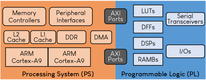
(b)

Figure 3: High-level architecture of (a) the Eyeriss ASIC [eyeriss] and (b) the Xilinx Zynq-7000 SoC FPGA [zynqs].

In this Dissertation, regarding “Hardware Acceleration”, we implement approximate arithmetic circuits using standard-cell libraries for ASIC. Our arithmetic circuits are also integrated in hardware DSP/AI functions, which are accelerated on standard-cell ASIC and Xilinx’s FPGAs. Moreover, we implement demanding CV kernels on the new European space-grade FPGAs. Finally, we accelerate custom DSP kernels, a sophisticated CV pipeline, and CNNs on Intel’s VPUs.

5 Heterogeneous Computing

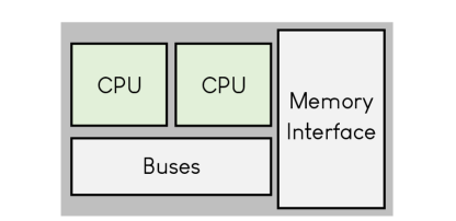
(a)

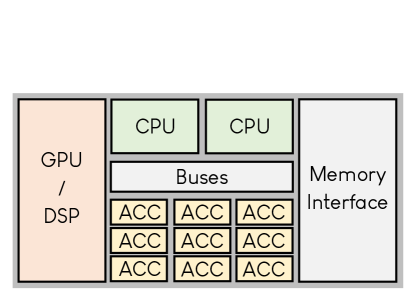
(c)

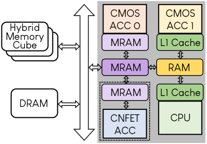
(d)

Figure 4: Evolution of heterogeneous computing architectures [moore_future]: (a) homogeneous CPU (past), (b) CPU + GPU/DSP (present), (c) CPU + GPU/DSP + accelerators (present), and (d) extreme heterogeneity in processors and memories (future).

The increased diversity of modern DSP/AI workloads in I/O, computational, and memory requirements has marginalized the use of homogeneous CPU-based computing platforms. To cope with all these requirements and provide efficient design solutions, the computing industry has turned to Heterogeneous Computing architectures [heter1, heterbook, heterog, heter2, heter3]. These architectures integrate more than one type of processor and potentially different memory technologies. In particular, contemporary heterogeneous architectures offer both general-purpose processors and specialized acceleration cores/engines. In terms of storage, the heterogeneity usually offers global memory, caches and scratchpad (working) memory. Figure 5 shows the evolution of heterogeneous architectures according to Shalf [moore_future]. Computing architectures with two similar CPUs or a multi-core CPU (Figure 4a) are now considered homogeneous systems. Currently, there are two prevailing kinds of computing architecture:

1. the heterogeneous architecture of Figure LABEL:fig_hh2, which combines the general-purpose CPU with a GPU/DSP accelerator [heterog].

2. the very heterogeneous architecture of Figure 4c, which additionally includes small accelerators (e.g., the VPU SoCs [myriad_vpu]).

The heterogeneity is expected to increase in the future (Figure 4d), integrating accelerators and memories of different technologies. The very heterogeneous architecture of Figure 4c is met in Intel’s Myriad VPUs [myriad_vpu], which constitute embedded SoCs for Edge Computing. These VPUs have recently emerged as an attractive solution for accelerating imaging applications with only $1$–$2$W. Compared to the CPU–GPU architectures, the VPU SoCs are more heterogeneous, as they offer general-purpose CPUs, vector cores, hardware filters for image processing, and a dedicated AI accelerator in the case of Myriad X.

Heterogeneous Computing imposes several challenges. From the developer side, the programming model involves parallel computing and mapping to specialized hardware, and thus, it is more complex than the respective one of conventional computing. The workloads need to be efficiently distributed and parallelized among the cores and accelerators to deliver improved performance and power efficiency. Towards this direction, the developer has to make decisions regarding the application’s decomposition into parallel computing tasks, the selection of the most suitable processor for each task, and the identification of the parts that offer limited parallelization opportunities or do not require acceleration. In the case of the Myriad VPUs, there are more technical challenges, given that these SoCs are mainly build for power efficiency rather than high performance. Therefore, the developer needs to exploit every piece of the VPU heterogeneity to provide sufficient performance.

In this Dissertation, regarding “Heterogeneous Computing”, we develop methodologies for the efficient mapping and scheduling of DSP/CV kernels and CNNs on the Myriad VPUs. We introduce several high- and low-level implementation techniques and evaluate the suitability of the VPUs as edge processors.

6 Scope and Contribution of Dissertation

The scope of the Dissertation is the design of arithmetic circuits and DSP & AI accelerators. In this context, we propose design solutions and methodologies for improving the efficiency of the implementations on ASIC/FPGA and multi-core SoCs. At circuit level, we adopt the promising design paradigm of Approximate Computing and propose new arithmetic approximation techniques, which are then used to design various approximate hardware accelerators on ASIC/FPGA technology. At platform level, we aim to unlock the full potential of new embedded devices, such as the space-grade FPGAs and the multi-core VPUs, by surpassing the bottlenecks of the tools and exploiting the heterogeneity of the SoCs, respectively, to accelerate high-performance DSP/AI workloads.

The main differentiation of the Dissertation compared to prior art is summarized as follows:

• At design technique level, we propose approximation methods that provide a larger approximation space, i.e., multiple approximation configurations, enabling to maximize the resource gains under a specified error constraint.

• At circuit level, we propose energy-efficient approximate circuits that can seamlessly adjust their approximation configuration at runtime.

• At hardware accelerator level, we perform an extensive design space exploration on approximation techniques, arithmetic formats, algorithms, and hardware design techniques to generate approximate ASIC/FPGA-based accelerators.

• At computing platform level, we systematically examine the capabilities of the programming tools and exploit the underlying hardware architectures to accelerate high-performance DSP/AI workloads.

The contribution of the Dissertation is summarized as follows:

• In Chapter 3, we report a comprehensive up-to-date literature survey for Approximate Computing, where we report the basic terminology, and then, classify and analyze the state-of-the-art software and hardware approximation techniques.

• In Chapter 4, we highlight the significance of the underlying arithmetic in circuits, and show that novel numerical formats and sophisticated bit-level optimizations can provide valuable resource gains in hardware.

• In Chapter 5, we address the circuit overheads of the classic high-radix encodings and propose a new approximate hybrid high-radix encoding, which is parametric in terms of approximation degree. This encoding is used to design the RAD family of approximate multipliers.

• In Chapter LABEL:chapter5, we introduce a low-overhead dynamic configuration scheme for adjusting the approximation degree of multipliers at runtime. This technique is applied in fixed- and floating-point arithmetic, generating the DyFXU and DyFPU families of runtime-configurable approximate multipliers.

• In Chapter LABEL:chapter6, we highlight the efficiency of integrating more than one approximation technique in the design of approximate circuits. In this context, we combine various state-of-the-art techniques and provide a very large design space for approximate multiplication. This extensive exploration results in the ROUP family of approximate multipliers, which form the state-of-the-art Pareto-front.

• In Chapter LABEL:chapter7, we introduce a methodology for designing approximate DSP/AI hardware accelerators. Based on this methodology, we fuse approximation techniques with various arithmetic formats, DSP/AI algorithms, and hardware design techniques, to generate energy-efficient hardware accelerators for 1D/2D signal processing and neural networks.

• In Chapter LABEL:chapter8, we introduce a methodology for efficiently mapping and accelerating high-performance DSP algorithms on the new European space-grade FPGAs. Based on this methodology, we apply our tool-level exploration to surpass issues that arise because the FPGA vendor is new and the space-grade FPGAs exhibit decreased flexibility compared to the commercial ones.

• In Chapter LABEL:chapter9, we introduce a methodology for partitioning, scheduling and optimizing demanding DSP and AI workloads on the heterogeneous multi-core VPUs. Based on this methodology, we exploit the full potential of the VPU SoCs to provide sufficient DSP and AI acceleration with limited power consumption.

7 Structure of Dissertation

The remainder of the Dissertation is organized as follows. Chapter 3 introduces the Approximate Computing paradigm, reviewing the terminology and state-of-the-art software & hardware approximation techniques. Chapters 4–LABEL:chapter9 report the main work of the Dissertation. Finally, Chapter LABEL:chapter10 concludes the Dissertation by summarizing the contributions and discussing future extensions. The structure of the main work is presented in Figure 5 and is divided in two parts:

Part 1:

“Arithmetic Approximation Techniques for Circuit Design”

Part LABEL:part2:

“Design Methodologies for Embedded Computing”

Part 1 includes Chapters 4–LABEL:chapter7 and focuses on arithmetic approximation techniques and the design of approximate DSP/AI hardware accelerators. Part LABEL:part2 includes Chapters LABEL:chapter8–LABEL:chapter9 and focuses on new embedded computing platforms (space-grade FPGAs and multi-core VPU SoCs) and the efficient acceleration of DSP/AI kernels. Both parts have a common goal: the development of energy-efficient DSP/AI accelerators. Part 1 reaches this goal from a lower design abstraction layer, while Part LABEL:part2 reaches it from higher design abstraction layers. Figure 6 depicts how we achieve this goal and what issues we have to surpass: (i) by using arithmetic approximations, while we have to care about the errors and application’s accuracy, (ii) via extensive and systematic tooling on the new space-grade FPGAs, where we have to surpass the limitations/issues of newly released tools/devices, (iii) by exploiting the heterogeneity of low-power multi-core VPUs, where we have to cope with resource-constrained edge devices and the increased complexity of the SoCs. Next, we discuss the content of each chapter included in Part 1 and Part LABEL:part2.

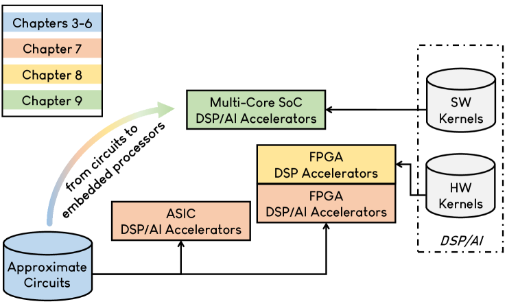
Figure 5: The structure of the Ph.D. Dissertation.

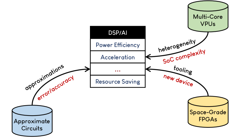
Figure 6: The goal of the Ph.D. Dissertation achieved through different design layers.

Chapter 4: This chapter acts as introductory to low-level logic optimizations, targeting to highlight the significance of studying the arithmetic of circuits/accelerators. For this purpose, it focuses on the Double Least Significant Bit (DLSB) numerical format, in which the numbers have an extra least significant bit, and it proposes sophisticated low-level optimizations. These bit manipulations are also used in the next chapters, and specifically in the design of approximate circuits. More explicitly, in this chapter, we improve the DLSB multiplication, resulting in decreased overheads versus the straightforward design approach. Moreover, as case study, we demonstrate how the proposed optimized circuit can be used as building block in the implementation of large-size multiplications.

Chapter 5: This chapter proposes an approximate hybrid high-radix encoding for generating the energy-efficient RAD multipliers. The proposed encoding scheme approximately encodes one of the operands, using the accurate radix-$4$ encoding for its most significant part and an approximate high-radix encoding for its least significant part. The approximation is inserted by mapping all the high-radix values to a set of values including only the $4$ largest powers of two. The proposed RAD family of approximate multipliers is configurable, and can be tuned to achieve the desired energy–accuracy trade-off.

Chapter LABEL:chapter5: This chapter proposes runtime-configurable approximate multipliers for fixed- and floating-point arithmetic. The approximation is inserted by two orthogonal techniques, i.e., partial product perforation and partial product rounding, which allow to integrate a low-overhead scheme for tuning the approximation at runtime. The runtime circuit variants DyFXU and DyFPU deliver negligible overhead versus their design-time counterparts (AxFXU and AxFPU). However, they still provide energy efficiency and benefit from their capability of selecting a different approximation configuration (among numerous ones) at runtime.

Chapter LABEL:chapter6: This chapter proposes the concept of cooperative approximation, namely, the application of more than one arithmetic approximation technique in the design of a circuit. The goal is twofold: (i) to create a very large approximation space that serves various design scenarios and can handle different error constraints or power budgets, and (ii) to identify the most efficient approximation solutions in terms of both accuracy and resources. Our extensive design space exploration results in $5$ new families of approximate multipliers, from which, ROUP is the most prominent, as it forms the state-of-the-art Pareto front with increased resolution.

Chapter LABEL:chapter7: This chapter introduces a methodology for the systematic development of approximate DSP/AI hardware accelerators. The proposed methodology consists of two stages, i.e., software-level exploration and hardware development. The main feature of the methodology is the combination of approximation techniques with different arithmetic formats (e.g., fixed/floating-point, quantized integer), alternative algorithms for the same application, and classic hardware design techniques. The goal of this chapter is twofold: (i) to assess the Dissertation’s approximate designs in real-world DSP/AI applications, and (ii) to evaluate the error resilience and quantify the resource gains of approximate DSP/AI accelerators.

Chapter LABEL:chapter8: This chapter proposes a design methodology for porting demanding DSP algorithms on the new European space-grade FPGAs. The methodology is divided with respect to the stages of the typical FPGA design flow. Our systematic design approach aids us to surpass issues that arise when using new tools or porting designs developed in other FPGA vendors, as well as confront the decreased flexibility and lower performance of space-grade FPGAs compared to their commercial counterparts. The evaluation is performed with hardware kernels for feature detection and stereo vision, and it includes comparisons to other FPGAs.

Chapter LABEL:chapter9: This chapter proposes a design methodology for the efficient mapping and acceleration of compute-intensive algorithms on the heterogeneous multi-core VPUs. The methodology aims to highlight the most efficient partitioning and scheduling schemes in such complex and very heterogeneous SoCs. In this context, we introduce several high- and low-level implementation techniques. Given that the VPUs are designed to provide low power consumption, our methodology and design choices allow us to deliver sufficient performance in custom DSP kernels and a sophisticated CV pipeline. Moreover, we deploy a demanding CNN. The evaluation includes comparison results with other state-of-the-art embedded devices.

Finally, even though all chapters are related to each other, they constitute standalone structures of text. Namely, each chapter has its own abstract, introduction, list of contributions, proposed techniques/designs/methodologies, experimental evaluation and conclusion.

8 Overview of Technologies, Tools and Devices

Table 1: Overview of Dissertation’s tools and devices.

Tool	Usage	Reference
Synopsys Design Compiler	standard-cell synthesis	Chapters 4–LABEL:chapter7
Synopsys PrimeTime	standard-cell power measurement	Chapters 4–LABEL:chapter7
Siemens QuestaSim	simulation (validation & power)	Chapters 4–LABEL:chapter8
Xilinx Vivado	FPGA implementation	Chapters LABEL:chapter7–LABEL:chapter8
Intel Quartus	FPGA implementation	Chapter LABEL:chapter8
Microsemi Libero	FPGA implementation	Chapter LABEL:chapter8
NanoXplore NXmap	FPGA implementation	Chapter LABEL:chapter8
Intel MDK	VPU implementation	Chapter LABEL:chapter9
Intel OpenVINO	VPU implementation	Chapter LABEL:chapter9
Google TensorFlow	CNN development	Chapters LABEL:chapter7,LABEL:chapter9

Device/Technology	Reference
TSMC Standard Cells (65-nm, 45-nm)	Chapters 4–LABEL:chapter7
Xilinx FPGAs (ZCU106, Zynq-7020)	Chapter LABEL:chapter7
Xilinx FPGA (Virtex-5QV)	Chapter LABEL:chapter8
Intel FPGA (Cyclone III)	Chapter LABEL:chapter8
Microsemi FPGA (RTG4)	Chapter LABEL:chapter8
NanoXplore FPGAs (NG-Medium, NG-Large)	Chapter LABEL:chapter8
Intel VPUs (Myriad 2, Myriad X, NCS2)	Chapter LABEL:chapter9
Nvidia GPU (Jetson Nano)	Chapter LABEL:chapter9

In this section, we report all the industrial-strength programming/development tools, devices/platforms and technologies that are used in the Dissertation. Table 1 summarizes all the relevant details. In Chapters 4–LABEL:chapter6, all the circuits are synthesized on TSMC standard-cell libraries (65-nm and 45-nm) with Synopsys’ Design Compiler tool. All the simulations are performed with Siemens’ (Mentor Graphics) QuestaSim, while for the power measurements, we use Synopsys’ PrimeTime. The same libraries and tools are used for the synthesis of the ASIC-based accelerators in Chapter LABEL:chapter7. Moreover, this chapter includes implementation results for accelerators on Xilinx’s ZCU106 and Zynq-7020 FPGAs, while the associated tool is Vivado. In Chapter LABEL:chapter8, we report numerous results from the implementation of DSP kernels on various FPGAs (Xilinx Virtex-5QV, Intel Cyclone III, and Microsemi RTG4). For these implementations, we use the corresponding software tool of each FPGA vendor. Chapter LABEL:chapter8 also includes results for NanoXplore’s new space-grade FPGAs (NG-Medium and NG-Large), which are generated by the NXmap tool. Chapter LABEL:chapter9 focuses on Intel’s VPUs (Myriad 2 and Myriad X), and all the implementations are performed with the associated tools, i.e., the MDK design suite for custom development and the OpenVINO framework for the deployment of neural networks. This chapter also reports results for Nvidia’s Jetson Nano GPU.

Chapter 3 The Approximate Computing Paradigm

The emergence of complex applications in domains applying multimedia processing and machine learning tasks has transformed the computing paradigm in embedded systems and data centers. These applications involve massive data and/or high computational complexity. Consequently, there is an emerging need for computational resources, which results in increasing more and more the power consumption of the computing systems. In the past, the technology scaling has played significant role towards surpassing these challenges, however, its declining efficiency pushes us to examine new computing paradigms. Approximate Computing is such an alternative paradigm, which trades-off accuracy loss and decreased quality of results for resource gains (e.g., in power/energy, area, latency, throughput). This computing paradigm is applied to error-resilient applications, such as those involving multimedia and machine learning, and it induces errors based on a disciplined approach to improve the efficiency of the systems/circuits and deliver the desired resource gains. Approximation opportunities abound in every layer of the typical computing stack, i.e., from transistors and circuits to compilers and programming languages. Therefore, there is a great variety of approximation techniques at each design abstraction layer, which study the errors and relax the accuracy from different perspective. In this chapter, we review state-of-the-art research works in Approximate Computing from all the layers of the computing stack. At first, we discuss the terminology of Approximate Computing and then, we classify and analyze the state-of-the-art approximation techniques with respect to their application layer (software or hardware). Our taxonomy is fine-grained, namely we study in-depth the approximation techniques of each layer and classify them based on their design approach. This chapter is based on our publications in [LeonSURV1, LeonSURV2].

1 Introduction

Approximate Computing covers the entire computing stack, i.e., approximation techniques are applied at all design abstraction layers. Significant research has been conducted in the field of software approximation techniques, which involve approximate programming languages, approximate compilers, approximation frameworks, quality-aware runtime systems, as well as approximations via precision scaling, task skipping and memoization. On the other hand, the most common hardware techniques target the modification of the circuits and hardware architectures, i.e., they generate a lossy circuit/architecture from the nominal accurate one. There is also wide research on the tunable scaling of the circuit’s voltage or frequency.

This chapter provides background in Approximate Computing. In particular, we introduce the terminology of Approximate Computing based on our literature search, and we report an extensive review of the state-of-the-art software and hardware approximation techniques. Our literature review includes newer works and more works compared to previous well-established surveys in Approximate Computing, i.e., from Mittal et al. (2016) [2016_Mittal_ACMsrv], Xu et al. (2016) [2016_Xu_IEEEdt], and Shafique et al. (2016) [Shafique_2016]. Furthermore, it differentiates from the survey of [2021_Stanley_ACMsrv], as it focuses on implementation details and analyzes the approximations of each reviewed technique.

The remainder of this chapter is organized as follows. Section 2 reports the terminology. Section 3 classifies and analyzes the software approximation techniques, while Section 4 classifies and analyzes the hardware approximation techniques.

2 The Terminology of Approximate Computing

Table 1: Basic terminology of Approximate Computing.

Term	Description
Error-Resilient Application	The application that tolerates errors and accepts results of lower quality.
Quality of Service	The quality of the results in terms of errors and accuracy.
Error Constraints	The quality/accuracy requirements that the results should satisfy.
Error Threshold	The maximum error allowed in the results.
Golden Result	The result that is obtained from the accurate computations.
Acceptable Result	The result that satisfies the application’s error constraints.
Variable Accuracy	The capability of providing different levels of accuracy.
Non-Critical Task	The task/computation that can be safely approximated due to its small impact on the quality of the output results.
Error Analysis	The study involving metrics, mathematics and simulations to examine the range, frequency, scaling, and propagation of errors.
Approximation Technique	The systematic and disciplined approach/method to insert computation errors in exchange for resource gains.
Approximation Degree	The strength of the approximation technique in terms of computations approximated and errors induced.
Approximation Configuration	An instance of the parameters/settings of the approximation technique.
Frozen Approximation	The approximation degree is fixed and cannot be re-configured.
Dynamic Approximation Tuning	The capability of adjusting the approximation degree at runtime to satisfy the desired error constraints.
Cross-Layer Approximation	The approximation that is applied at multiple design abstraction layers (software, hardware, architecture).
Heterogeneous Approximation	The approximation that concurrently applies multiple configurations of different degree within the same system.
Approximation Space Exploration	The study involving error analysis and gain quantification to examine trade-offs and select the suitable approximations.
Approximation Localization	The systematic approach to locate the computations and regions that are offered for approximation.
Error Modeling	The process of emulating the errors of the approximations.
Error Prediction	The process of predicting errors before computing the final result.
Error Detection	The process of identifying an error occurrence.
Error Compensation	The process of modifying the erroneous result to reduce the error.
Error Correction	The process of correcting the erroneous result.

Table 1 describes the most frequently used terms in Approximate Computing. The term error is used to indicate that the output result is different from the accurate result (produced with conventional computing). Error is distinguished from fault, which refers to an unexpected condition (e.g., stuck-at-logic in circuits, bit-flips in memories, faults in operating systems) that causes the system to unintentionally output erroneous results. Another significant term is accuracy, which is defined as the distance between the approximate and the (nominal) accurate result and is expressed with various error metrics (e.g., error rate, mean relative error, mean squared error, classification accuracy). Accuracy is distinguished from precision, which expresses the differentiation between nearby discrete values and does not refer to errors of Approximate Computing but to quantization noise (inserted by the real-to-digital value mapping). More specifically, in computer arithmetic, the more bits are used for the decimal number part, the higher the precision, i.e., there are more bits for the representation and the numbers are closer to their real value. Moreover, in Approximate Computing, the term Quality-of-Service (QoS) is used to describe the overall quality of the results (in terms of accuracy and errors), considering the expected/accurate results as baseline and the application’s quality constraints.

3 Classification of Software Approximation Techniques

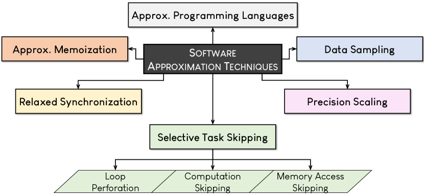
Figure 1: Classification of state-of-the-art software approximation techniques.

In this section, we classify and introduce approximation techniques that are applied at software level, i.e., the higher level of the design abstraction hierarchy. The goal of software Approximate Computing is to improve the execution time of the program and/or the energy consumption of the system. The techniques of the literature, illustrated in Figure 1, can be categorized into six classes: (i) Selective Task Skipping, (ii) Approximate Memoization, (iii) Relaxed Synchronization, (iv) Precision Scaling, (v) Data Sampling, and (vi) Approximate Programming Languages. Typical techniques include some of the following features: approximation libraries/frameworks, compiler extensions, accuracy tuning tools, runtime systems, and language annotations. Moreover, there are numerous techniques allowing the programmer to specify QoS constraints, provide approximate code variants, and mark the program’s regions/tasks for approximation.

The remainder of this section reports representative state-of-the-art works for software Approximate Computing. Besides classifying state-of-the-art techniques, we discuss their approximations and how they are applied. Table 2 reports the references of all the reviewed research works. We note that the literature also includes entire approximation frameworks, such as ACCEPT [2015_Sampson_UOW] and OPPROX [2017_Mitra_CGO], which integrate multiple of these state-of-the-art techniques. Their goal is to perform an extensive exploration using differing approximation approaches, identify the best approximation opportunities, and hence, maximize the resource gains while satisfying the application’s/user’s constraints.

Table 2: Classification of software approximation techniques.

SW Approximation Class	References
Loop Perforation	[2009_Hoffmann_MIT, 2010_Misailovic_ICSE, 2011_Sidiroglou_FCE, 2015_Shi_IEEEcal, 2017_Omar_ICCD, 2018_Li_ICS, 2020_Baharvand_IEEEtetc, 2015_Tan_ASP-DAC, 2018_Kanduri_DAC]
Computation Skipping	[2009_Meng_IPDPS, 2010_Byna_GPGPU, 2015_Raha_DATE, 2015_Vassiliadis_PPoPP, 2016_Vassiliadis_CGO, 2006_Rinard_ICS, 2007_Rinard_OOPSLA, 2017_Lin_ISCAS, 2018_Akhlaghi_ISCA]
Memory Access Skipping	[2014_Miguel_MICRO, 2016_Yazdanbakhsh_ACMtaco, 2018_Kislal_ELSEclss, 2013_Samadi_MICRO, 2019_Karakoy_ACMmacs, 2015_Zhang_DATE]
Approximate Memoization	[2011_Chaudhuri_FSE, 2014_Samadi_ASPLOS, 2014_Mishra_WACAS, 2017_Brumar_IPDPS, 2015_Keramidas_WAPCO, 2018_Tziantzioulis_IEEEmicro, 2005_Alvarez_IEEEtc, 2013_Rahimi_IEEEtcasii, 2018_Zhang_IEEEcal, 2019_Liu_ISCA]
Relaxed Synchronization	[2012_Renganarayana_RACES, 2012_Misailovic_RACES, 2013_Misailovic_ACMtecs, 2015_Campanoni_CGO, 2020_Stitt_ACMtecs, 2010_Sreeram_IISWC, 2010_Mengt_IPDPS, 2012_Rinard_RACES]
Precision Scaling	[2011_Dinechin_IEEEtc, 2010_Linderman_CGO, 2017_Chiang_POPL, 2017_Darulova_ACMtoplas, 2013_Rubio_SC, 2018_Guo_ISSTA, 2013_Lam_ICS, 2018_Lam_SAGE, 2014_Chiang_PPoPP, 2016_Rubio_ICSE, 2018_Yesil_IEEEmicro, 2015_Tian_GLSVLSI, 2018_Menon_SC, 2020_Brunie_SC, 2019_Laguna_HPC, 2020_Kang_CGO]
Data Sampling	[2012_Laptev_VLDB, 2015_Goiri_ASPLOS, 2019_Hu_MASCOTS, 2017_Quoc_MIDDL, 2016_Krishnan_WWW, 2017_Quoc_ATC, 2018_Wen_ICDCS, 2013_Agarwal_EuroSys, 2016_Kandula_MOD, 2016_Zhang_VLDB, 2016_Anderson_ICDE, 2019_Park_MOD]
Approximate Program. Languages	[2011_Ansel_CGO, 2007_Sorber_SenSys, 2010_Baek_PLDI, 2015_Boston_OOPSLA, 2012_Carbin_PLDI, 2013_Carbin_OOPSLA, 2014_Misailovic_OOPSLA, 2011_Liu_ASPLOS, 2015_Achour_OOPSLA, 2011_Sampson_PLDI, 2015_Park_FSE, 2014_Park_GIT, 2008_Goodman_UAI, 2014_Mansinghka_CoRR, 2016_Tolpin_IFL, 2014_Bornholt_ASPLOS, 2014_Sampson_PLDI, 2019_Fernando_ACMpapl, 2019_Joshi_ICSE]

1 Selective Task Skipping

Loop Perforation

The loop perforation technique skips some of the loop iterations in a software program to provide performance/energy gains in exchange for QoS loss. Subsequently, we present several relevant works [2009_Hoffmann_MIT, 2010_Misailovic_ICSE, 2011_Sidiroglou_FCE, 2015_Shi_IEEEcal, 2017_Omar_ICCD, 2018_Li_ICS, 2020_Baharvand_IEEEtetc, 2015_Tan_ASP-DAC, 2018_Kanduri_DAC] involving design space exploration on loop perforation with programming frameworks and profiling tools.

Starting with one of the first state-of-the-art works, the SpeedPress compiler [2009_Hoffmann_MIT] supports a wide range of loop perforation types, i.e., modulo, truncation, and randomized. It takes as input the original source code, a set of representative inputs, as well as a programmer-defined QoS acceptability model, and it outputs a loop perforated binary. In the same context, Misailovic et al. [2010_Misailovic_ICSE] propose a QoS profiler to identify computations that can be approximated via loop perforation. The proposed profiling tool searches the space of loop perforation and generates results for multiple perforation configurations. In [2011_Sidiroglou_FCE], the same authors propose a methodology to exclude critical loops, i.e., whose skipping results in unacceptable QoS, and they perform exhaustive and greedy design space explorations to find the Pareto-optimal perforation configurations for a given QoS constraint.

In [2015_Shi_IEEEcal], the authors propose an architecture that employs a profiler to identify non-critical loops towards their perforation. To protect code segments that can be affected by the perforated loops, the architecture is equipped with HaRE, i.e., a hardware resilience mechanism. Another interesting work is GraphTune [2017_Omar_ICCD], which is an input-aware loop perforation scheme for graph algorithms. This approach analyzes the input dependence of graphs to build a predictive model that finds near-optimal perforation configurations for a given accuracy constraint. Li et al. [2018_Li_ICS] propose a compiling & profiling system, called Sculptor, to improve the conventional loop perforation, which skips a static subset of iterations. More specifically, Sculptor dynamically skips a subset of the loop instructions (and not entire iterations) that do not affect the output accuracy. More recently, the authors of [2020_Baharvand_IEEEtetc] develop LEXACT, which is a tool for identifying non-critical code segments and monitoring the QoS of the program. LEXACT searches the loop perforation space, trying to find perforation configurations that satisfy pre-defined metrics.

The loop perforation technique has also been used in approximation frameworks for heterogeneous multi-core systems combining various approximation mechanisms. Tan et al. [2015_Tan_ASP-DAC] propose a task scheduling algorithm, which employs multiple approximate versions of the tasks with loops perforated. Kanduri et al. [2018_Kanduri_DAC] target applications in which the main computations are continuously repeated, and they tune the loop perforation at runtime.

Computation Skipping

This technique omits the execution of blocks of codes with respect to the acceptable QoS loss, programmer-defined constraints, and/or runtime predictions regarding the output accuracy [2009_Meng_IPDPS, 2010_Byna_GPGPU, 2015_Raha_DATE, 2015_Vassiliadis_PPoPP, 2016_Vassiliadis_CGO, 2006_Rinard_ICS, 2007_Rinard_OOPSLA, 2017_Lin_ISCAS, 2018_Akhlaghi_ISCA]. Compared to loop perforation, these techniques do not focus only on skipping loop iterations, but also skip higher-level computations/tasks e.g., an entire convolution operation. Most of the state-of-the-art works perform application-specific computation skipping.

Meng et al. [2009_Meng_IPDPS] introduce a parallel template to develop approximate programs for iterative-convergence recognition & mining algorithms. The proposed programming template provides several strategies (implemented as libraries) for task dropping, such as convergence-based computation pruning, computation grouping in stages, and early termination of iterations. Another interesting work involving application-specific computation skipping is presented in [2010_Byna_GPGPU]. The authors of this work study the error tolerance of the supervised semantic indexing algorithm to make approximation decisions. Regarding their task dropping approach, they choose to omit the processing of common words (e.g., “the”, “and”) after the initial iterations, as these computations have negligible impact on accuracy.

The authors of [2015_Raha_DATE] propose two techniques to find computations with low impact on the QoS of the Reduce-and-Rank computation pattern, targeting to approximate or skip them completely. To identify these computations, the first technique uses intermediate reduction results and ranks, while the second one is based on the spatial or temporal correlation of the input data (e.g., adjacent image pixels or successive video frames). Similar to the other state-of-the-art works, Vassiliadis et al. [2015_Vassiliadis_PPoPP, 2016_Vassiliadis_CGO] propose a programming environment that skips (or approximates) computations with respect to programmer-defined QoS constraints. More specifically, the programmer expresses the significance of the tasks using pragmas directives, optionally provides approximate variants of tasks, and specifies the task percentage to be executed accurately. Based on these constraints, the proposed system makes decisions at runtime regarding the approximation/skipping of the less significant tasks.

Rinard [2006_Rinard_ICS] builds probabilistic distortion models based on linear regression to study the impact of computation skipping on accuracy. The programmer partitions the computations into tasks, which are then marked as “critical” or “skippable” through random skip executions. The probabilistic models estimate the output distortion as function of the skip rates of the skippable tasks. This approach is also applied in parallel programs [2007_Rinard_OOPSLA], where probabilistic distortion models are employed to tune the early phase termination at barrier synchronization points, targeting to keep all the parallel cores busy.

Significant research has also been conducted on skipping the computations of Convolutional Neural Networks (CNNs). Lin et al. [2017_Lin_ISCAS] introduce PredictiveNet to predict the sparse outputs of the nonlinear layers and skip a large subset of convolutions at runtime. The proposed technique, which does not require any modification in the original CNN structure, examines the most-significant part of the convolution to predict if the nonlinear layer output is zero, and then it decides whether to skip the remaining least-significant part computations or not. In the same context, Akhlaghi et al. [2018_Akhlaghi_ISCA] propose SnaPEA, exploiting the convolution–activation algorithmic chain in CNNs (activation inputs the convolution result and outputs zero if it is negative). This technique early predicts negative convolution results, based on static re-ordering of the weights and monitoring of the partial sums’ sign bit, in order to skip the rest computations.

Memory Access Skipping

Another approach to improve the execution time and energy consumption at software level is the memory access skipping. Such techniques [2014_Miguel_MICRO, 2016_Yazdanbakhsh_ACMtaco, 2018_Kislal_ELSEclss, 2013_Samadi_MICRO, 2019_Karakoy_ACMmacs, 2015_Zhang_DATE] aim to avoid high-latency memory operations, while as a result, they also reduce the number of computations.

Miguel et al. [2014_Miguel_MICRO] exploit the approximate data locality to skip the required memory accesses due to L1 cache miss. In particular, they employ a load value approximator, which learns value patterns using a global history buffer and an approximator table, to estimate the memory data values. RFVP [2016_Yazdanbakhsh_ACMtaco] uses value prediction instead of memory accessing. When selected load operations miss in the cache memory, RFVP predicts the requested vales without checking for misprediction or recovering the values. As a result, timing overheads from pipeline flushes and re-executions are avoided. Furthermore, a tunable rate of cache misses is dropped after the value prediction to eliminate long memory stalls. The authors of [2018_Kislal_ELSEclss] propose a framework that skips costly last-level cache misses according to a programmer-defined error constraint and an heuristic predicting skipped data.

To improve the performance of CUDA kernels on GPUs, Samadi et al. [2013_Samadi_MICRO] propose a runtime approximation framework, called SAGE, which focuses on optimizing the memory operations among other functionalities. The approximations lie in skipping selective atomic operations (used by kernels to write shared variables) to avoid conflicts leading to performance decrease. Furthermore, SAGE reduces the number of memory accesses by packing the read-only input arrays, and thus, allowing to access more data with fewer requests. Karakoy et al. [2019_Karakoy_ACMmacs] propose a slicing-based approach to identify data (memory) accesses that can be skipped to deliver energy/performance gains within an acceptable error bound. The proposed method applies backward and forward code slicing to estimate the gains from skipping each output data. Moreover, the ‘$0$’ value is used for each data access that is not performed. The ApproxANN framework [2015_Zhang_DATE], apart from performing approximate computations, skips memory accesses on neural networks according to the neuron criticality. More specifically, a theoretical analysis is adopted to study the impact of neurons on the output accuracy and characterize their criticality. The neuron approximation under a given QoS constraint is tuned by an iterative algorithm, which applies the approximations and updates the criticality of each neuron (it may change due to approximations in other neurons).

2 Approximate Memoization

The memoization technique stores results of previous calculations or pre-computed values in memory to use them instead of performing calculations. Namely, this memory functions as a look-up table, which maps a set of data identifiers to a set of stored data. Subsequently, we focus on approximate memoization techniques [2011_Chaudhuri_FSE, 2014_Samadi_ASPLOS, 2014_Mishra_WACAS, 2017_Brumar_IPDPS, 2015_Keramidas_WAPCO, 2018_Tziantzioulis_IEEEmicro] relying on software frameworks, compilers and programmer’s decisions. Nevertheless, we note that there are also approaches [2005_Alvarez_IEEEtc, 2013_Rahimi_IEEEtcasii, 2018_Zhang_IEEEcal, 2019_Liu_ISCA] requiring hardware modification to support memoization.

Chadhuri et al. [2011_Chaudhuri_FSE] propose an approximate memoization for computations in loops. Prior executing an expensive function within a loop, this technique checks a look-up table to find if this computation was previously performed for similar input data. In this case, the cached result is used, otherwise, the function is executed and the new computation is stored in the look-up table. Paraprox [2014_Samadi_ASPLOS] is a software framework for identifying common patterns in data-parallel programs and applying tailored approximations. For the Map & Scatter/Gather patterns, Paraprox uses memoization rather than performing computations. In particular, it fills a look-up table with pre-computed data, which are obtained from the execution of the Map & Scatter/Gather function for some representative inputs, and it performs runtime look-up table queries instead of the conventional computations.

iACT [2014_Mishra_WACAS] is another approximation framework that applies runtime memoization among other functionalities. The programmer uses pragmas to declare the functions for memoization and specify the error tolerance percentage. For each function call-site, the framework creates a global table to store pairs of function arguments and output results. In case the function arguments are already stored in the table (within an error bound), the corresponding output results are returned. Otherwise, the function is accurately executed and the new input–output pairs are stored in the table. The ATM approach [2017_Brumar_IPDPS] performs runtime task memoization, relying on hashing functions to store the task inputs and an adaptive algorithm to automatically decide whether to use memoization or execute the task. The programmer needs to use pragmas to specify the tasks that are suitable for memoization. The authors of [2015_Keramidas_WAPCO] introduce an approximate memoization mechanism for GPU fragment shading operations, which reduces the precision of the input parameters and performs partial matches. To identify approximate memoization opportunities, they characterize various fragment shader instructions in terms of memoization hits and output accuracy. Moreover, runtime policies are proposed to tune the precision according to the errors introduced.

Contrary to the aforementioned techniques, TAF-Memo [2018_Tziantzioulis_IEEEmicro] is an output-based function memoization technique, i.e., it memoizes function calls based on their output history. TAF-Memo checks for temporal locality by calculating the relative arithmetic difference of two consecutive output values from the same function call-site. In case this difference is below the acceptable error constraint, memoization is applied by returning the last computed output for the following function calls.

3 Relaxed Synchronization

The execution of parallel applications on multi/many-core systems requires time-consuming synchronization to either access shared data or satisfy data dependencies. The literature includes various techniques [2012_Renganarayana_RACES, 2012_Misailovic_RACES, 2013_Misailovic_ACMtecs, 2015_Campanoni_CGO, 2020_Stitt_ACMtecs, 2010_Sreeram_IISWC, 2010_Mengt_IPDPS, 2012_Rinard_RACES] that relax the conventional synchronization requirements guaranteeing error-free execution, to improve the performance.

The authors of [2012_Renganarayana_RACES] propose the four-step RaC methodology to systematically relax synchronization, while always satisfying a programmer-defined QoS constraint. Initially, the programmer specifies the parallel code segments, and then applies the RaC methodology. This methodology identifies criteria for quantifying the acceptable QoS, selects the relaxation points, modifies the code to enable the execution of both the original and relaxed versions, and selects the suitable relaxation degree (i.e., which instances to relax for each synchronization point). Misailovic et al. [2012_Misailovic_RACES] propose the Dubstep system, which relaxes the synchronization of parallelized programs based on a “find-transform-navigate” approach. Dubstep performs a profiling-based analysis of the original program to find possible optimizations, inserts opportunistic synchronization and barriers, and finally, performs an exploration including accuracy, performance and safety analysis.

QuickStep [2013_Misailovic_ACMtecs] is a system for approximately parallelizing sequential programs without preserving their semantics within statistical accuracy bounds. Among other transformations, QuickStep replicates shared objects to eliminate the bottlenecks of synchronized operations on them. HELIX-UP [2015_Campanoni_CGO] is another parallelizing compiler that selectively relaxes strict adherence to program semantics to tackle runtime performance bottlenecks, involving profiling and user interaction to tune QoS. The compiler also offers a synchronization-relaxing knob to decrease the inter-core communication overhead by synchronizing sequential segments with prior iterations. More recently, the authors of [2020_Stitt_ACMtecs] introduce PANDORA, which is an approximate parallelizing framework based on symbolic regression machine learning and sampled outputs of the original function. To avoid timing bottlenecks, such as data movement and synchronization, and improve parallelism, PANDORA eliminates loop-carried dependencies using fitness functions and constraints regarding error and performance. In [2010_Sreeram_IISWC], the authors exploit the concept of approximate shared value locality to reduce synchronization conflicts in programs using optimistic synchronization. The reduction of conflicts on approximately local variables, detected for a given similarity constraint, is achieved through an arbitration mechanism that imprecisely shares the values between threads. The authors of [2010_Mengt_IPDPS] apply aggressive coarse-grained parallelism on recognition & mining algorithms by relaxing or even ignoring data dependencies between different iterations. As a result, the timing overheads are reduced in comparison with the conventional parallel implementation, which also applies parallelization only within the iteration (iterations are executed serially). Rinard [2012_Rinard_RACES] introduces synchronization-free updates to shared data structures by eliminating the conventional use of mutual exclusion and dropping array elements at the worst scenario. Moreover, the same work applies relaxed barrier synchronization, allowing the threads to pass the barrier without stalling to wait for the other threads.

4 Precision Scaling

Precision scaling (tuning) refers to the discipline reduction of the nominal numerical precision, resulting in improved calculation speed and/or memory bandwidth [2020_Cherubin_ACMsrv]. The state-of-the-art software-level works [2011_Dinechin_IEEEtc, 2010_Linderman_CGO, 2017_Chiang_POPL, 2017_Darulova_ACMtoplas, 2013_Rubio_SC, 2018_Guo_ISSTA, 2013_Lam_ICS, 2018_Lam_SAGE, 2014_Chiang_PPoPP, 2016_Rubio_ICSE, 2018_Yesil_IEEEmicro, 2015_Tian_GLSVLSI, 2018_Menon_SC, 2020_Brunie_SC, 2019_Laguna_HPC, 2020_Kang_CGO] address several challenges, such as the scaling degree, scaling automation, mixed precision, and dynamic scaling.

Starting with works based on formal methods to reduce the precision and examine the errors, the Gappa tool [2011_Dinechin_IEEEtc] automates the study of rounding errors in elementary functions and floating-point calculations using interval arithmetic. An extended version of this tool is Gappa++ [2010_Linderman_CGO], which provides automated analysis of numerical errors in a wide range of computations, i.e., fixed-point, floating-point, linear and non-linear. This tool integrates several features, such as operation rewriting to facilitate the isolation of rounding errors, and affine arithmetic to accurately bound linear calculations with correlated errors. FPTuner [2017_Chiang_POPL] is a tool that performs formal error analysis based on symbolic Taylor expansions and quadratically constrained quadratic programming. It searches for precision allocations that satisfy constraints such as the number of operators at a given precision and the number of type casts. Rosa [2017_Darulova_ACMtoplas] is a source-to-source compiler that combines satisfiability modulo theories with interval arithmetic to bound the round-off errors of the fixed- and floating-point formats.

Several works employ heuristics and automated search to scale the precision of floating-point programs. Precimonious [2013_Rubio_SC] searches all the program variables in their order of declaration using the delta-debugging algorithm, and it lowers their precision according to an error constraint specified by the programmer. In the same context, HiFPTuner [2018_Guo_ISSTA] firstly groups dependent variables that may require the same precision, and then it performs a customized hierarchical search. Lam et al. [2013_Lam_ICS] introduce a framework that employs the breadth-first search algorithm to identify code regions that can tolerate lower precision. Similar to this technique, CRAFT [2018_Lam_SAGE] performs binary searches to initially determine the required program precision, and then truncate the results of some of the floating-point instructions. Towards the detection of large floating-point errors, the authors of [2014_Chiang_PPoPP] propose S${}^{3}$FP. This tool is based on an heuristic-guided search to find the inputs causing the largest errors. The Blame Analysis [2016_Rubio_ICSE] combines concrete and shadow execution to generate a blame set for the program instructions, which contains the minimum precision requirements under a giver error constraint. This approach can be also used in cooperation with the previous search-based works, and specifically, as pre-processing to reduce the search space. Schkufza et al. [2014_Schkufza_PLDI] treat the scaling of floating-point precision as a stochastic search problem. In particular, they repeatedly apply random program transformations and use a robust search to guarantee the maximum errors.

The concept of dynamic precision scaling, i.e., the precision tuning at runtime with respect to the input data and error tolerance, has been studied in [2018_Yesil_IEEEmicro]. The dynamic scaling framework of this work integrates an offline application profiler, a runtime monitor to track workload changes, and an accuracy controller to adjust the precision accordingly. ApproxMA [2015_Tian_GLSVLSI] dynamically scales the precision of data memory accesses in algorithms such as mixture model-based clustering. This framework integrates a runtime precision controller, which generates custom bit-widths according to the QoS constraints, and a memory access controller, which loads the scaled data from memory. The custom bit-widths are generated by analyzing a subset of data and intermediate results and calculating metrics regarding the error appearance and the number of tolerable errors.

Mixed floating-point precision has also been studied in high-performance computing workloads. ADAPT [2018_Menon_SC] uses algorithmic differentiation, i.e., a technique for numerically evaluating the derivative of a function corresponding to the program, to estimate the output error of high-performance computing workloads. It provides a precision sensitivity profile to guide the development of mixed-precision programs. The authors of [2020_Brunie_SC] propose an instruction-based search that explores information about the dynamic program behaviour and the temporal locality.

To enable mixed floating-point precision in GPUs, the authors of [2019_Laguna_HPC] propose the GPUMixer tool, which relies on static analysis to find code regions where precision scaling improves the performance. Next, GPUmixer performs a dynamic analysis involving shadow computations to examine if the scaled program configurations satisfy the accuracy constraints. In the same context, PreScaler [2020_Kang_CGO] is an automatic framework that generates precision-scaled OpenCL programs, considering both kernel execution and data transfer. Initially, it employs a system inspector to collect information about precision scaling on the target platform, and an application profiler to identify memory objects with floating-point elements for potential scaling. This information is exploited by a decision maker, which finds the best scaling configuration using decision tree search on a minimized space.

5 Data Sampling

Approximate Computing is also exploited in big data analysis, in an effort to reduce the increased number of computations due to the large amount of data. The key idea is to perform computations on a representative data sample instead of the entire dataset. In this context, data sampling methods [2012_Laptev_VLDB, 2015_Goiri_ASPLOS, 2019_Hu_MASCOTS, 2017_Quoc_MIDDL, 2016_Krishnan_WWW, 2017_Quoc_ATC, 2018_Wen_ICDCS, 2013_Agarwal_EuroSys, 2016_Kandula_MOD, 2016_Zhang_VLDB, 2016_Anderson_ICDE, 2019_Park_MOD] provide real-time processing with error bounds in applications involving stream analytics, database search, and model training.

EARL [2012_Laptev_VLDB] is an extension of Hadoop (i.e., a software framework that provides distributed storage and big data processing on clusters), which delivers early results with reliable error bounds. It applies statistics-based uniform sampling from distributed files. Goiri et al. [2015_Goiri_ASPLOS] propose the ApproxHadoop framework to generate approximate MapReduce programs based on task dropping and multi-stage input sampling. They also bound the errors using statistical theories. The programmer tunes the approximation by specifying either the ratio of task dropping and/or input sampling or the desired error bound. Similarly, ApproxSpark [2019_Hu_MASCOTS] performs sampling at multiple arbitrary points of long chains of transformations to facilitate the aggregation of huge amounts of data. This framework models the clustering information of transformations as a data provenance tree, and then it computes the approximate aggregate values as well as error thresholds. Moreover, the sampling rates are dynamically selected according to programmer-specified error thresholds.

Sampling methods have also been examined in stream analytics. StreamApprox [2017_Quoc_MIDDL] is an approximate stream analytics system that supports batched and pipelined stream processing. It employs two sampling techniques (stratified and reservoir sampling) to approximate the outputs with rigorous error bounds. IncApprox [2016_Krishnan_WWW] combines approximate and incremental computations to provide stream analytics with bounded error. This system executes a stratified sampling algorithm that selects data for which the results have been memoized from previous runs, and it adjusts the computations to produce an incrementally updated output. On the other hand, PrivApprox [2017_Quoc_ATC] combines sampling and randomized response to provide approximate computations and privacy guarantee. This system integrates a query execution interface that systematically explores the trade-off between accuracy and query budget. ApproxIoT [2018_Wen_ICDCS] facilitates approximate stream analytics at the edge by combining stratified reservoir sampling and hierarchical processing.

A variety of sampling methods have been employed in approximate query processing systems for databases. BlinkDB [2013_Agarwal_EuroSys] performs approximate distributed query processing, supporting SQL-based aggregation queries with time and error constraints. It creates stratified samples based on past queries and uses an heuristic-based profiler to dynamically select the sample that meets the query’s constraints. Another system applying approximate big-data queries is Quickr [2016_Kandula_MOD], which integrates operators sampling multiple join inputs into a query optimizer, and then it searches for an appropriate sampled query plan. Sapprox [2016_Zhang_VLDB] is a distribution-aware system that employs the occurrences of sub-datasets to drive the online sampling. In particular, the exponential number of sub-datasets is reduced to a linear one using a probabilistic map, and then, cluster sampling with unequal probability theory is applied for sub-dataset sampling. Sapprox also determines the optimal sampling unit size in relation with approximation costs and accuracy.

Numerous works use data sampling to decrease the increased computational cost of model training for machine learning applications. Zombie [2016_Anderson_ICDE] is a two-stage system that trains approximate models based on clustering and active learning. The first stage applies offline indexing to organize the dataset into index groups of similar elements. Afterwards, the stage of online querying uses the index groups that are likely to output useful features to create the training subset of data. BlinkML [2019_Park_MOD] approximately trains a model on a small sample, while providing accuracy guarantees. The sample is obtained through uniform random sampling, however, in case of very large datasets, a memory-efficient algorithm is employed.

6 Approximate Programming Languages

The high-level approximation of software programs has been examined through approximate programming languages, i.e., language extensions that allow the programmer to systematically declare approximate code regions, variables, loops, and functions, insert randomness in the program, and/or specify error constraints. The literature involves numerous works [2011_Ansel_CGO, 2007_Sorber_SenSys, 2010_Baek_PLDI, 2015_Boston_OOPSLA, 2012_Carbin_PLDI, 2013_Carbin_OOPSLA, 2014_Misailovic_OOPSLA, 2011_Liu_ASPLOS, 2015_Achour_OOPSLA, 2011_Sampson_PLDI, 2015_Park_FSE, 2014_Park_GIT, 2008_Goodman_UAI, 2014_Mansinghka_CoRR, 2016_Tolpin_IFL, 2014_Bornholt_ASPLOS, 2014_Sampson_PLDI, 2019_Fernando_ACMpapl, 2019_Joshi_ICSE] that enable approximate procedural, object-oriented, and probabilistic programming.

Ansel et al. [2011_Ansel_CGO] introduce a set of PetaBricks language extensions that allow the programmer to write code of variable accuracy. These extensions expose the performance–accuracy trade-off to the compiler, which automatically searches the algorithmic space to tune the program according to the programmer’s accuracy constraints. Eon [2007_Sorber_SenSys] is a programming language that allows the programmer to annotate program flows (paths) with different energy states. The Eon runtime system predicts the workload and energy of the system, and then it adjusts the execution of flows according to the programmer’s declarations and the energy constraints. In the same context, Baek and Chilimbi [2010_Baek_PLDI] propose Green, which is a two-phase programming framework providing language extensions to approximate expensive functions and loops. The programmer uses pragma-like annotations to specify approximate variants of functions. In the calibration phase, Green builds a model to quantify the QoS loss and the performance/energy gains. This model is then used in the operational phase to generate an approximate program satisfying the programmer’s QoS constraint. DECAF [2015_Boston_OOPSLA] is a type-based approximate programming language that allows the programmer to specify the correctness probability for some of the program variables. The DECAF type system also integrates solver-aided type inference to automatically tune the type of the rest variables, code specialization, and dynamic typing. Flikker [2011_Liu_ASPLOS] provides language annotations to mark the program variables and partition the data into critical and non-critical regions (stored in unreliable memories). Topaz [2015_Achour_OOPSLA] is a task-based language that maps tasks onto approximate hardware and uses an outlier detector to find and re-execute the computations producing unacceptable results.

In [2012_Carbin_PLDI], the authors introduce language constructs for generating approximate programs and proof rules for verifying the acceptability properties. Rely [2013_Carbin_OOPSLA] is an imperative language that allows the programmer to introduce quantitative reliability specifications for generating programs with data stored in approximate memory and inexact arithmetic/logical operations. Chisel [2014_Misailovic_OOPSLA] automates the selection of Rely’s approximations while satisfying the programmer-defined reliability and accuracy constraints. To solve this optimization problem, Chisel employs an integer programming solver. All these works include safety analysis and program verification for sequential programs. In contrast, Parallely [2019_Fernando_ACMpapl] is a programming language for approximating parallel programs through canonical sequentialization, i.e., a verification method that generates sequential programs capturing the semantics of parallel programs.

Targeting approximations in Java programs, the authors of [2011_Sampson_PLDI] propose EnerJ, i.e., a language extension providing type qualifiers to specify data that can be approximately stored or computed. EnerJ guarantees isolation of the approximate computations. FlexJava [2015_Park_FSE] offers another set of language extensions to annotate approximate programs. Using an approximation safety analysis, FlexJava automates the approximation of data and operations while ensuring safety guarantees. ExpAX [2014_Park_GIT] allows the programmer to explicitly specify error expectations for a subset of Java. Based on an approximation safety analysis, it identifies operations that are candidate for approximation, and then, an heuristic-based framework approximates those that statistically satisfy the error expectations.

Significant research has also been conducted on probabilistic programming languages. Church [2008_Goodman_UAI] is a probabilistic language that inserts randomness on a deterministic function subset using stochastic functions. The Church semantics are defined in terms of evaluation histories and conditional distributions on the latter. Similarly, Venture [2014_Mansinghka_CoRR] is another language that enables the specification of probabilistic models and inference problems. The Anglican [2016_Tolpin_IFL] language and runtime system provides probabilistic evaluation model and functional representations, e.g., distributions and sequences of random variables.

Uncertain$\scriptstyle<$T$\scriptstyle>$ [2014_Bornholt_ASPLOS] is a language abstraction that manipulates data as probability distributions. Random variables are declared as “uncertain” and a Bayesian network for representing computations is build, where nodes correspond to the variables and edges correspond to conditional variable dependencies. The Uncertain$\scriptstyle<$T$\scriptstyle>$ runtime system performs hypothesis tests and sampling to evaluate the network. Similarly, Sampson et al. [2014_Sampson_PLDI] use probabilistic assertions on random variables. Their tool, called MayHap, performs probabilistic evaluation by statically building a Bayesian representation network based on the input distribution and dynamically interpreting it via sampling. In the same context, AxProf [2019_Joshi_ICSE] is a profiling-based framework for analyzing randomized approximate programs. The programmer specifies probabilistic predicates for the output, i.e., regarding the expectation of the output value and/or the probability that the output satisfies a condition, and AxProf generates approximate programs based on statistical tests.

4 Classification of Hardware Approximation Techniques

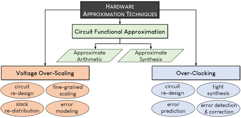
Figure 2: Classification of state-of-the-art hardware approximation techniques.

In this section, we classify and introduce the hardware approximation techniques, which are applied at the lower level of the design abstraction hierarchy. These techniques aim to improve the area, power consumption, and performance of the circuits i.e., the basic building blocks of accelerators, processors, and computing platforms. The hardware approximation techniques can be categorized into three classes: (i) Circuit Functional Approximation (CFA), (ii) Voltage Over-Scaling (VOS), and (iii) Over-Clocking (OC). In approximate hardware, we distinguish two types of errors: the functional errors (produced by CFA) and the timing errors (produced by VOS and OC). Figure 2 illustrates the hardware approximation techniques, including a further taxonomy to sub-classes.

In the remainder of this section, we present state-of-the-art works, organized according to the proposed classification. Table 3 summarizes the state-of-the-art hardware approximation techniques. We also note that some works belong to more than one sub-class, however, we opt to assign them to the sub-class of their prevalent technique and highlight the relevant features.

Table 3: Classification of hardware approximation techniques.

HW Approximation Class	Technique/Approach
Adder Approximation	use of approximate full adder cells [2013_Gupta_IEEEtcad, 2013_Yang_NANO, 2018_Pashaeifar_IEEEtvlsi, 2018_Dalloo_IEEEtvlsi]
	segmentation and carry prediction [2013_Kim_ICCAD, 2015_Hu_DATE, 2012_Kahng_DAC, 2013_Ye_ICCAD, 2015_Shafique_DAC, 2018_Akbari_IEEEtcasii, 2018_Xu_IEEEtvlsi, 2020_Ebrahimi_IEEEtcasii]
Multiplier Approximation	truncation and rounding [2015_Hashemi_ICCAD, 2017_Zendegani_IEEEtvlsi, LeonMicro, LeonTECS, 2019_Vahdat_IEEEtvlsi, LeonDAC, 2020_Frustaci_IEEEtcasii]
	approximate radix encodings [2017_Liu_IEEEtc, 2019_Venkatachalam_IEEEtc, 2016_Jiang_IEEEtc, 2020_Waris_IEEEtcasii, LeonTVLSI]
	use of approximate compressors [2015_Momeni_IEEEtc, 2017_Akbari_IEEEtvlsi, 2019_Sabetzadeh_IEEEtcasi, 2018_Esposito_IEEEtcasi, 2020_Strollo_IEEEtcasi]
	logarithmic approximation [2018_Liu_IEEEtcasi, 2020_Saadat_DATE, 2021_Ansari_IEEEtc, 2021_Pilipovic_IEEEtcasi]
Divider Approximation	bit-width scaling [2016_Hashemi_DAC, 2019_Jiang_IEEEtc]
	use of approximate adder/subtractor cells [2015_Chen_GLSVLSI, 2016_Chen_IEEEtc, 2018_Chen_IEEEtmscs, 2020_Adams_IEEEtc]
	simplification of computations [2016_Zendegani_DATE, 2017_Vahdat_DATE, 2019_Imani_Date, 2018_Liu_ARITH, 2019_Saadat_DAC]
Approximate Synthesis	structural netlist transformation [2017_Schlachter_IEEEtvlsi, 2018_Scarabottolo_DATE, 2013_Venkataramani_DATE, 2017_Liu_ICCAD, 2021_Castro_IEEEtcasii]
	Boolean rewriting [2012_Venkataramani_DAC, 2014_Ranjan_DATE, 2013_Miao_ICCAD, 2018_Hashemi_DAC]
	high-level approximate description [2015_Yazdanbakhsh_DATE, 2014_Nepal_DATE, 2017_Lee_DATE, 2019_Nepal_IEEEtetc, 2020_Castro_ICCAD]
	evolutionary synthesis [2013_Sekanina_ICES, 2015_Vasicek_IEEEtec, 2017_Mrazek_DATE, 2016_Vasicek_FPL, 2019_Vasicek_DATE]
Voltage Over-Scaling	slack re-distribution [2010_Kahng_ASP-DAC]
	circuit re-design and architecture modification [2011_Mohapatra_DATE, 2013_Chen_IEEEtvlsi, 2018_Zhang_DAC]
	fine-grained scaling [2019_Pandey_DAC, 2020_Wang_IEEEtc, 2019_Zervakis_IEEEtcasii]
	error modeling [2010_Liu_IEEEtvlsi, 2012_Jeon_IEEEtcasii, 2017_Ragavan_DATE, 2020_Jiao_IEEEtcad, 2018_Zervakis_IEEEtvlsi]
Over-Clocking	tight synthesis [2018_Alan_IEEEtcad]
	circuit re-design and architecture modification [2013_Ramasubramanian_DAC, 2014_Shi_DAC, 2017_Wang_IEEEtvlsi]
	error detection & correction [2014_Choudhury_IEEEtc, 2016_Ragavan_ISVLSI, 2017_Li_IEEEtvlsi]
	error prediction [2012_Roy_DAC, 2015_Constantin_DATE, 2016_Jiao_ICCD, 2017_Jiao_DATE]

1 Circuit Functional Approximation

Circuit functional approximation modifies the original accurate design by reducing its circuit complexity at logic level. Typical CFA approaches include: (i) the modification of the circuit’s truth table, (ii) the use of an approximate version of the initial hardware algorithm, (iii) the use of small inexact components as building blocks, and (iv) approximate circuit synthesis. The main target of CFA is the arithmetic circuits [2020_Jiang_IEEE], as they constitute the key processing units of processors and accelerators, and thus, they inherently affect the power efficiency and performance of the entire system. Interestingly, the literature provides several open-source libraries of approximate arithmetic circuits, such as ApproxAdderLib [2015_Shafique_DAC], EvoApprox8b [2017_Mrazek_DATE] and SMApproxLib [2018_Ullah_DAC]. In this literature review, we focus on approximate adders, multipliers, and dividers. However, we note that numerous works design and evaluate other approximate arithmetic operations, such as circuits for multiply-accumulate [2019_Chen_IEEEtc, 2019_Gillani_IEEEa], square root [2019_Jiang_IEEEtc], squaring [2020_Manikanta_IEEEtvlsi], square-accumulate [2018_Gillani_IEEEa], and Coordinate Rotation Digital Computer (CORDIC) [2017_Chen_IEEEtscl]. Moreover, the literature includes automated methods for generating approximate circuits, which are presented in the context of approximate logic synthesis.

Approximate Adders

Significant research has been conducted on the design of approximate area- and power-efficient adders. The approximation techniques for inexact adders involve: (i) use of approximate full adder cells [2013_Gupta_IEEEtcad, 2013_Yang_NANO, 2018_Pashaeifar_IEEEtvlsi, 2018_Dalloo_IEEEtvlsi] and (ii) segmentation and carry prediction [2013_Kim_ICCAD, 2015_Hu_DATE, 2012_Kahng_DAC, 2013_Ye_ICCAD, 2015_Shafique_DAC, 2018_Akbari_IEEEtcasii, 2018_Xu_IEEEtvlsi, 2020_Ebrahimi_IEEEtcasii]. In the following, we present representative state-of-the-art works with approximate adders.

The IMPACT adders are based on inexact full adder cells, which are approximated at the transistor level to deliver up to 45% area reduction [2013_Gupta_IEEEtcad]. Another transistor-level cell approximation is proposed in [2013_Yang_NANO], where the AXA 4-transistor XOR/XNOR-based adders are implemented, delivering up to $31\%$ gain in dynamic power consumption. Moreover, in [2018_Pashaeifar_IEEEtvlsi], approximate reverse carry-propagate full adders are used to build the hybrid RCPA adders. Targeting higher level approximations, the OLOCA adder splits the addition into accurate and approximate segments [2018_Dalloo_IEEEtvlsi], and for the latter, it employs OR gates for the most-significant bit additions and outputs constant ‘$1$’ for the least-significant ones. To reduce the worst-case carry propagation delay, Kim et al. [2013_Kim_ICCAD] propose a carry prediction scheme leveraging the less-significant input bits, which is $2.4\times$ faster than the conventional ripple-carry adder. Similarly, Hu et al. [2015_Hu_DATE] introduce a carry speculating method to segment the carry chain in their design, which also performs error and sign correction. Compared to the accurate adder, the proposed design is $4.3\times$ faster and saves $47\%$ power.

The quality constraint of applications may vary during runtime, thus, research efforts have also focused on designing dynamically configurable adders, which can tune their accuracy. In [2012_Kahng_DAC], the authors propose an accuracy-configurable adder, called ACA, which consists of several sub-adders and an error detection & correction module. The design controls the accuracy at runtime and can operate in accurate mode. Another dynamically configurable adder, called GDA, is proposed in [2013_Ye_ICCAD], where multiplexers select the carry input either from the previous sub-adder or the carry prediction unit, providing a more graceful degradation of the accuracy. In the same direction, the GeAr adder employs multiple sub-adders of equal length to variable approximation modes [2015_Shafique_DAC]. This architecture also supports accurate mode via a configurable error correction unit.

More recently, Akbari et al. [2018_Akbari_IEEEtcasii] introduce the RAP-CLA adder, which splits the conventional carry look-ahead scheme into two segments, i.e., the approximate part and the augmenting part, supporting approximate and accurate mode. When operating at the approximate mode, the augmenting part is power-gated to reduce power consumption. Another carry-prediction-based approach supporting both modes is the SARA design [2018_Xu_IEEEtvlsi]. This adder uses carry ripple sub-adders, and the carry prediction does not require a dedicated circuitry. Finally, the BSCA adder, which is based on a block-based carry speculative approach [2020_Ebrahimi_IEEEtcasii], integrates an error recovery unit and non-overlapped blocks consisting of a sub-adder, a carry prediction unit, and a selection unit.

Approximate Multipliers

The multiplication circuits have attracted significant interest from the research community. The literature includes a plethora of inexact multipliers, which can be categorized according to the prevailing approximation techniques: (i) truncation and rounding [2015_Hashemi_ICCAD, 2017_Zendegani_IEEEtvlsi, LeonMicro, LeonTECS, 2019_Vahdat_IEEEtvlsi, LeonDAC, 2020_Frustaci_IEEEtcasii], (ii) approximate radix encodings [2017_Liu_IEEEtc, 2019_Venkatachalam_IEEEtc, 2016_Jiang_IEEEtc, 2020_Waris_IEEEtcasii, LeonTVLSI], (iii) use of approximate compressors [2015_Momeni_IEEEtc, 2017_Akbari_IEEEtvlsi, 2019_Sabetzadeh_IEEEtcasi, 2018_Esposito_IEEEtcasi, 2020_Strollo_IEEEtcasi], and (iv) logarithmic approximation [2018_Liu_IEEEtcasi, 2020_Saadat_DATE, 2021_Ansari_IEEEtc, 2021_Pilipovic_IEEEtcasi]. Subsequently, we introduce the state-of-the-art works from each category.

Starting with the rounding and truncation techniques, the DRUM multiplier [2015_Hashemi_ICCAD] dynamically reduces the input bit-width, based on the leading ‘$1$’ bits, to achieve $60\%$ power gain in exchange for mean relative error of $1.47\%$. Zendegani et al. [2017_Zendegani_IEEEtvlsi] propose the RoBa multiplier, which rounds the operands to the nearest exponent-of-two and performs a shift-based multiplication in segments. In [LeonMicro], the PR approximate multiplier perforates partial products and applies rounding to the remaining ones, delivering up to $69\%$ energy gains. The same approximation technique is integrated in the mantissa multiplication of floating-point numbers to create the AFMU multiplier [LeonTECS]. Vahdat et al. [2019_Vahdat_IEEEtvlsi] propose the TOSAM multiplier, which truncates the input operands according to their leading ‘$1$’ bit. To decrease the error, the truncated values are rounded to the nearest odd number. In [LeonDAC], different rounding, perforation and encoding schemes are combined to extract the most energy-efficient designs. Finally, Frustaci et al. [2020_Frustaci_IEEEtcasii] implement an alternative dynamic truncation with correction, along with an efficient mapping for the remaining partial product bits.

Next, we present multipliers generating their partial products based on approximate radix encodings. Liu et al. [2017_Liu_IEEEtc] modify the Karnaugh map of the radix-4 encoding to create approximate encoders for generating the least-significant partial product bits. A similar approach is followed in [2019_Venkatachalam_IEEEtc], where approximate radix-4 partial product generators are designed. Jiang et al. [2016_Jiang_IEEEtc] use an approximate adder to generate the $\pm$3$\times$ multiplicand term in the radix-8 multiplier. In [2020_Waris_IEEEtcasii], the authors propose a hybrid low-radix encoding, which encodes the most-significant bits with the accurate radix-4 encoding and the least-significant bits with the proposed approximate radix-8 encoding. Correspondingly, the hybrid high-radix encoding, i.e., accurate radix-4 and approximate radix-2${}^{k}$, is examined in [LeonTVLSI].

Several works employ approximate compressors for the partial product accumulation. Momeni et al. [2015_Momeni_IEEEtc] modify the truth table of the accurate 4:2 compressor to create two simplified designs and use them in the Dadda multiplier. The authors in [2017_Akbari_IEEEtvlsi] design 4:2 compressors, again for Dadda multipliers, which can switch between accurate and approximate mode at runtime, providing 68% lower power consumption. In [2019_Sabetzadeh_IEEEtcasi], an approximate 4:2 compressor is implemented in FinFET based on a three-input majority gate, and then it is used in the Dadda architecture along truncation. Esposito et al. [2018_Esposito_IEEEtcasi] introduce a new family of approximate compressors and assign them to each column of the partial product matrix according to their allocation algorithm. Another interesting work is the design of approximate compressors for multipliers using the concept of stacking circuit [2020_Strollo_IEEEtcasi].

Regarding the approximate logarithmic multipliers, Liu et al. [2018_Liu_IEEEtcasi] employ a truncated binary-logarithm converter and inexact adders for the mantissa addition to design the ALM family of multipliers. The logarithmic-based REALM multiplier [2020_Saadat_DATE] partitions the power-of-two intervals of the input operands into segments, and determines an error compensation factor for each one. The ILM multiplier [2021_Ansari_IEEEtc] differentiates from the conventional design, as it rounds the input operands to their nearest power-of-two using a nearest ‘$1$’ bit detector. Pilipovic et al. [2021_Pilipovic_IEEEtcasi] propose a two-stage trimming logarithmic multiplier, which reduces at first the bit-width of the input operands, and then the bit-width of the mantissas.

Approximate Dividers

The division circuits have received less attention than the other arithmetic circuits (adders and multipliers), even though they feature complex calculations. Nevertheless, the literature provides numerous works aiming to reduce the large critical paths of the conventional dividers. The approximation techniques for the division circuits can be categorized as follows: (i) bit-width scaling [2016_Hashemi_DAC, 2019_Jiang_IEEEtc], (ii) use of approximate adder/subtractor cells [2015_Chen_GLSVLSI, 2016_Chen_IEEEtc, 2018_Chen_IEEEtmscs, 2020_Adams_IEEEtc], and (iii) simplification of computations [2016_Zendegani_DATE, 2017_Vahdat_DATE, 2019_Imani_Date, 2018_Liu_ARITH, 2019_Saadat_DAC].

The first class of approximation techniques uses exact dividers with reduced bit-width. The approximate divider of [2016_Hashemi_DAC] dynamically selects the most relevant bits from the input operands and performs accurate division at lower bit-width, providing up to $70\%$ power gains in exchange for $3\%$ average error. The design makes use of leading ‘$1$’ bit detectors, priority encoders, multiplexers, subtractor and barrel shifter. Similarly, the AAXD divider of [2019_Jiang_IEEEtc] detects the leading ‘$1$’ bits and uses a pruning scheme to extract the bits that will be given as input to the divider. Additionally, the design integrates an error correction unit to form the final output.

Regarding the second class of approximation techniques, Chen et al. [2015_Chen_GLSVLSI] perform the subtraction of the non-restoring array divider with inexact subtractor circuits employing pass transistor logic. For the proposed divider, called AXDnr, the authors examine different schemes with regard to which subtractions of the division array to approximate. Similarly, in the AXDr divider of [2016_Chen_IEEEtc], some of the subtractions of the restoring array divider are performed with inexact subtractor circuits. The use of inexact cells has also been examined in the high radix SRT divider [2018_Chen_IEEEtmscs]. In this divider, called HR-AXD, the inexact cell is a signed-digit adder, which is employed based on different replacement schemes and along with cell truncation and error compensation. More recently, Adams et al. [2020_Adams_IEEEtc] introduce two approximate division architectures, called AXRD-M1 and AXRD-M2, which deliver up to 46% area and 57% power gains, respectively, compared to the exact restoring divider. The first design replaces some of the restoring divider cells with inexact ones of simplified logic, while the second one involves the elimination of some rows of the divider.

Targeting to perform the division with simplified computations, the SEERAD divider [2016_Zendegani_DATE] rounds the divisor to a specific form based on the leading ‘$1$’ bit position, and thus, the division is transformed to shift-&-add multiplication. Similarly, Vahdat et al. [2017_Vahdat_DATE] propose the TruncApp divider, which replaces the division with the multiplication of the truncated dividend by the approximate inverse divisor. In the same context, the CADE divider of [2019_Imani_Date] performs the floating-point division by subtracting the input mantissas. To compensate a large error, which is estimated by analyzing the most-significant input bits, a pre-computed value is retrieved from memory. In [2018_Liu_ARITH], the proposed AXHD divider approximates the least-significant computations of the division using a non-iterative logarithmic approach that is based on leading ‘$1$’ bit detection and subtraction of the logarithmic mantissas. Finally, Saadat et al. [2019_Saadat_DAC] propose approximate integer and floating-point dividers with near-zero error bias, called INZeD and FaNZeD, respectively, by combining an error correction method with the classical approximate logarithmic divider.

Approximate Synthesis

An automated approach to generate inexact circuits is the approximate logic synthesis. This method provides increased approximation diversity, i.e., multiple approximate variants of circuits, without relying on the manual approximation inserted by the designer, such as in the case of the aforementioned arithmetic approximations. Another benefit of approximate synthesis is that several techniques generate the approximate variant that leads to the maximum hardware gains for a given approximation/error constraint. The state-of-the-art techniques can be categorized as follows [2020_Scarabottolo_IEEE]: (i) structural netlist transformation [2017_Schlachter_IEEEtvlsi, 2018_Scarabottolo_DATE, 2013_Venkataramani_DATE, 2017_Liu_ICCAD, 2021_Castro_IEEEtcasii], (ii) Boolean rewriting [2012_Venkataramani_DAC, 2014_Ranjan_DATE, 2013_Miao_ICCAD, 2018_Hashemi_DAC], (iii) high-level approximate description [2015_Yazdanbakhsh_DATE, 2014_Nepal_DATE, 2017_Lee_DATE, 2019_Nepal_IEEEtetc, 2020_Castro_ICCAD], and (iv) evolutionary synthesis [2013_Sekanina_ICES, 2015_Vasicek_IEEEtec, 2017_Mrazek_DATE, 2016_Vasicek_FPL, 2019_Vasicek_DATE].

Several works of the literature employ a direct acyclic graph to represent the circuit netlist, where each node corresponds to a gate. In this context, the GLP technique [2017_Schlachter_IEEEtvlsi] prunes nodes with an iterative greedy approach according to their impact on the final output and their toggle activity. In contrast, the CC framework [2018_Scarabottolo_DATE] performs an exhaustive exploration of all possible node subsets that can be pruned without surpassing the error constraint. Venkataramani et al. [2013_Venkataramani_DATE] propose SASIMI, which is based on a greedy heuristic to find signal pairs assuming the same value and substitute one with the other. This automatic synthesis framework guarantees that the user-defined quality constraint is satisfied and generates accuracy configurable circuits. To apply stochastic netlist transformation, the SCALS framework [2017_Liu_ICCAD] maps an initial gate-level network to the targeted technology (standard cell or FPGA), and then it iteratively extracts sets of sub-netlists and inserts random approximations in them. These sub-netlists are evaluated using statistical hypothesis testing. More recently, Castro-Codinez et al. [2021_Castro_IEEEtcasii] propose the AxLS framework, which converts the Verilog netlist to XML format and then applies typical transformation techniques, e.g., gate pruning, according to an error threshold.

The second category includes techniques that apply approximations in a formal Boolean representation of the circuit before it is synthesized. The SALSA approach [2012_Venkataramani_DAC] encodes the error constraints into a quality logic function, which compares the outputs of the accurate and approximate circuits. Towards logic simplification, SALSA computes the “observability don’t cares” for each output of the approximate circuit, i.e., the set of input values for which the output is insensitive. In the same direction, but for sequential circuits, Ranjan et al. [2014_Ranjan_DATE] introduce ASLAN. This framework generates several approximate variants of the combinational blocks, and then it identifies the best approximations for the entire sequential circuit based on a gradient-descent approach. Miao et al. [2013_Miao_ICCAD] use a two-phase Boolean minimization algorithm to address the problem of approximate synthesis. The first phase solves the problem under a given constraint for the error magnitude, and the second phase iteratively finds a solution that also satisfies the error frequency constraint. In an iterative fashion, the BLASYS methodology [2018_Hashemi_DAC] partitions the circuit into smaller circuits, and for each one, it generates an approximate truth table based on Boolean matrix factorization. The approximate sub-circuits are synthesized and the trade-off between error and power/area efficiency for the entire circuit is evaluated.

Regarding approximations introduced at the hardware description level, Yazdanbakhsh et al. [2015_Yazdanbakhsh_DATE] propose the Axilog language annotations, which provide syntax and semantics for approximate design and reuse in Verilog. Axilog allows the designer to partition the design into accurate and approximate segments. ABACUS [2014_Nepal_DATE] is another interesting work, which parses the behavioral/RTL Verilog description of the design to create its abstract syntax tree. Next, a set of diverse transformations is applied to the tree to create approximate variants, which are then written in Verilog. An expanded version of ABACUS is introduced in [2019_Nepal_IEEEtetc], where sorting-based evolutionary algorithms are employed for design space exploration. Moreover, the new ABACUS version focuses on approximations in critical paths to facilitate the reduction of the supply voltage. Lee et al. [2017_Lee_DATE] generate approximate designs in Verilog from C accurate descriptions. The proposed framework computes data statistics and mobility information for the given design and employs an heuristic solver for optimizing the energy–quality trade-off. Targeting to high-level synthesis, the AxHLS approach [2020_Castro_ICCAD] performs a design space exploration, based on analytical models, to identify the best arithmetic approximations for a given error constraint. Starting from a C description, AxHLS adopts scheduling and binding operations to apply the approximations provided by the exploration and generate the Verilog code.

The fourth class of techniques for automated synthesis of approximate circuits is based on evolutionary algorithms, i.e., heuristic-based search algorithms that treat circuit approximation as multi-objective optimization problem and generate a set of solutions. In this context, Sekanina et al. [2013_Sekanina_ICES] use Cartesian genetic programming to minimize the error in adders considering the number of logic gates as constraint. This approach is extended in [2015_Vasicek_IEEEtec], where approximate multipliers and median filters are evolved through randomly seeded Cartesian genetic programming. Based on the same utilities, the authors of [2017_Mrazek_DATE] propose the EvoApprox8b library of approximate adders and multipliers. This library is generated by examining various trade-offs between accuracy and hardware efficiency, and it offers different approximation variants and circuit architectures. In [2016_Vasicek_FPL], a search-based technique for evolutionary circuit synthesis for FPGAs is proposed. In particular, this approach represents the circuit as a directed acyclic graph, and re-synthesizes approximate configurations based on Cartesian genetic programming. Vasicek et al. [2019_Vasicek_DATE] adjust the approximation degree according to the significance of the inputs. To do so, they adopt a weighted error metric to determine the significance of each input vector and use Cartesian genetic programming to minimize the circuit’s area while satisfying a threshold.

2 Voltage Over-Scaling

Voltage over-scaling reduces the circuit’s supply voltage below its nominal value, while keeping the clock frequency constant. The circuit operation at a lower voltage value produces timing errors due to the failure of the critical paths to meet the delay constraints. Nevertheless, considering that power consumption depends on the voltage value, VOS techniques are continuously examined in the literature. An exploration and quantification of the benefits and overheads of VOS is presented in [2010_Kurdahi_IEEEtvlsi]. Research involving VOS can be classified in the following categories: (i) slack re-distribution [2010_Kahng_ASP-DAC], (ii) circuit re-design and architecture modification [2011_Mohapatra_DATE, 2013_Chen_IEEEtvlsi, 2018_Zhang_DAC], (iii) fine-grained scaling [2019_Pandey_DAC, 2020_Wang_IEEEtc, 2019_Zervakis_IEEEtcasii], and (iv) error modeling [2010_Liu_IEEEtvlsi, 2012_Jeon_IEEEtcasii, 2017_Ragavan_DATE, 2020_Jiao_IEEEtcad, 2018_Zervakis_IEEEtvlsi].

Kahng et al. [2010_Kahng_ASP-DAC] shift the timing slack of the frequently executed near-critical paths through slack redistribution, and thus, they reduce the minimum voltage at which the error rate remains acceptable. The proposed technique is based on post-layout cell resizing to deliver the switching activity-aware slack redistribution. More specifically, a heuristic finds the voltage satisfying the desired error rate, and then it increases the transistor width of the cells to optimize the frequently executed paths.

In [2011_Mohapatra_DATE], the authors optimize building blocks for more graceful degradation under VOS, using two techniques, i.e., dynamic segmentation & error compensation and delay budgeting of chained datapath. The first technique bit-slices the datapath of the adder and employs a multi-cycle error correction circuitry that tracks the carries. The second technique adds transparent latches between chained arithmetic units to distribute the clock period. To facilitate VOS, Chen et al. [2013_Chen_IEEEtvlsi] build their designs on the residue number system, which provides shorter critical paths than conventional arithmetic. They also employ the reduced precision redundancy scheme to eliminate the timing errors. Another interesting work is Thundervolt [2018_Zhang_DAC], which provides error recovery in the Multiply-And-Accumulate (MAC) units of systolic Deep Neural Network (DNN) accelerators. To detect timing errors, Thundervolt employs Razor shadow flip-flops. In case an error occurs in a MAC, a multiplexer forwards the previous MAC’s accurate partial sum (stored in the Razor flip-flop) to the next MAC.

Targeting fine-grained VOS solutions, i.e., different voltages across the same circuit architecture, Pandey et al. propose GreenTPU [2019_Pandey_DAC]. This design integrates a timing error control unit in each MAC row of the systolic array, which stores input sequences producing timing errors. As a result, when such an input sequence pattern is identified, the voltage of the MAC is scaled accordingly to prevent timing errors. In the same context, the authors of [2020_Wang_IEEEtc] propose NN-APP. This framework analyzes the error propagation in neural networks to model the impact of VOS on accuracy. Based on this analysis, as well as an error resilience study for the neurons, NN-APP uses a voltage clustering method to assign the same voltage to neurons with similar error resilience. Another fine-grained VOS approach is proposed in [2019_Zervakis_IEEEtcasii]. This framework provides voltage heterogeneity by using a greedy algorithm to solve the optimization problem of grouping and assigning the voltage of arithmetic units to different islands.

The analysis of errors in circuits under VOS is considered a key factor, as it guides the aggressiveness of voltage scaling towards the acceptable error margins. In [2010_Liu_IEEEtvlsi], an analytical method to study the errors in voltage over-scaled arithmetic circuits is proposed. Similarly, the authors of [2012_Jeon_IEEEtcasii] introduce a probabilistic approach to model the errors of the critical paths. In the same category, we include works relying on simulations to analyze the errors of VOS. Ragavan et al. [2017_Ragavan_DATE] characterize arithmetic circuits in terms of energy efficiency and errors using transistor-level SPICE simulation for various voltages. Based on this characterization, they propose a statistical model to simulate the behavior of arithmetic operations in VOS systems. Exploiting the machine learning methods, Jiao et al. [2020_Jiao_IEEEtcad] propose LEVAX to model voltage over-scaled functional units. This input-aware model is trained on data from gate-level simulations to predict the timing error rate for each output bit. To provide accurate VOS-aware gate-level simulation, Zervakis et al. propose VOSsim [2018_Zervakis_IEEEtvlsi]. This framework performs an offline characterization of the flip-flop for timing violations and calculates the cell delays for the targeted voltage, enabling gate-level simulation under VOS.

3 Over-Clocking

Over-clocking (or frequency over-scaling) configures the circuit/system at higher clock frequencies than those that respect the critical paths. As a result, timing errors are induced in exchange for increased performance. A trade-off analysis between accuracy and performance when over-clocking FPGA-based designs is presented in [2013_Shi_FCCM]. In the same work, the authors show that OC outperforms the traditional bit truncation for the same error constraint. For our analysis, we consider that the state-of-the-art works of the domain focus on the following directions: (i) tight synthesis [2018_Alan_IEEEtcad], (ii) circuit re-design and architecture modification [2013_Ramasubramanian_DAC, 2014_Shi_DAC, 2017_Wang_IEEEtvlsi], (iii) error detection & correction [2014_Choudhury_IEEEtc, 2016_Ragavan_ISVLSI, 2017_Li_IEEEtvlsi], and (iv) error prediction [2012_Roy_DAC, 2015_Constantin_DATE, 2016_Jiao_ICCD, 2017_Jiao_DATE].

The first approach aims to reduce the timing errors of OC by optimizing the critical paths of the design. In this context, the SlackHammer framework [2018_Alan_IEEEtcad] synthesizes circuits with tight delay constraints to reduce the number of near-critical paths, and thus, decrease the probability of timing errors when frequency is over-scaled. At first, SlackHammer isolates the paths and identifies potential delay optimizations. Based on the isolated path analysis, the framework performs an iterative synthesis with tighter constraints for the primary outputs with negative slack.

The second class of techniques modifies the conventional circuit architecture to facilitate frequency OC and increase the resilience to timing errors. The retiming technique [2013_Ramasubramanian_DAC] re-defines the boundaries of combinational logic by moving the flip-flops backward or forward between the stages. Based on this circuit optimization, the synthesis is relaxed by ignoring the paths that are bottleneck to minimum period retiming. Targeting different circuit architectures, Shi et al. [2014_Shi_DAC] adopt an alternative arithmetic, called online, and show that online-based circuits are more resilient to the timing errors of OC than circuits with traditional arithmetic. The modification of the initial neural network model to provide resilience in timing errors has also attracted research interest. In this direction, Wang et al. [2017_Wang_IEEEtvlsi] propose an iterative reclocking-and-retraining framework for operating neural network circuits at higher frequencies under a given accuracy constraint. The clock frequency is gradually increased and the network’s weights are updated through back-propagation training until to find the maximum frequency for which the timing errors are mitigated and the accuracy constraint is satisfied.

Several works propose circuits for timing error detection & correction, enabling the use of over-clocking. These techniques either improve the frequency value of the first failure, i.e., the first timing error, or reduce the probability of timing errors. TIMBER [2014_Choudhury_IEEEtc] masks timing errors by borrowing time from successive pipeline stages. According to this approach, the use of discrete time-borrowing flip-flops and continuous time-borrowing latches slows down the appearance of timing errors with respect to the frequency scaling. Ragavan et al. [2016_Ragavan_ISVLSI] detect and correct timing errors by employing a dynamic speculation window on the double-sampling scheme. This technique adds an extra register (called shadow and clocked by a second “delayed” clock) at the end of the pipelined path to sample the output data at two different time instances. The proposed approach also uses an online slack measurement to adaptively over-clock the design. The TEAI approach [2017_Li_IEEEtvlsi] is based on the locality of the timing errors in software-level instructions, i.e., the tendency of specific instructions to produce timing errors. TEAI identifies these instructions at runtime, and sends error alarms to hardware, which is equipped with error detection & correction circuits.

There is also wide research on the prediction of the timing errors in advance, which allows to over-scale the frequency according to the acceptable error margins. In [2012_Roy_DAC], the authors introduce an instruction-level error prediction system for pipelined micro-processors, which stalls the pipeline when critical instructions are detected. Their method is based on gate-level simulations to find the critical paths that are sensitized during the program execution. Similarly, Constantin et al. [2015_Constantin_DATE] obtain the maximum delays for each arithmetic instruction through gate-level simulations, and they dynamically exploit timing margins to apply frequency over-scaling.

Besides instruction-level prediction models, there are numerous works that build models based on machine learning and simulations of functional units. A representative work of this approach is WILD [2016_Jiao_ICCD], which builds a workload-dependent prediction model using logistic regression. In the same direction, SLoT [2017_Jiao_DATE] is a supervised learning model that predicts timing errors based on the inputs and the clock frequency. At first, SLoT performs gate-level simulation to extract timing class labels, i.e., “timing error” or “no timing error”, for different inputs and frequencies. These classes are then used, along with features extracted from random data pre-processing, to train the error prediction model.

Part 1 Arithmetic Approximation Techniques for Circuit Design

Chapter 4 Arithmetic Optimization: Double-LSB Encoding

Computer arithmetic has received significant attention, as it inherently affects the efficiency and performance of the hardware accelerators. In this context, novel numerical formats are examined, targeting to provide increased resource gains compared to the conventional binary formats in various application domains, e.g., in Digital Signal Processing (DSP). In this chapter, we adopt the Double Least Significant Bit (DLSB) format, where the numbers have an extra least significant bit, and we apply optimizations in the multiplication, i.e., one of the most resource-hungry DLSB operations. The DLSB arithmetic delivers several benefits, such as the symmetric representation range, the number negation performed only by bitwise inversion, the improvement of the residue number circuits, and the improvement of the rounding process in floating-point calculations. However, all these advantageous features come with some penalties in the design of the arithmetic DLSB units. Towards reducing the DLSB overheads in the multiplication, we propose an energy-efficient scheme for multiplying $\mathit{2}$’s-complement binary numbers, which is based on sophisticated bit-level manipulations. The overhead of the proposed DLSB design is negligible compared to the conventional design for ordinary $\mathit{2}$’s-complement numbers, i.e., $\mathit{\scriptstyle\sim}$$\mathit{3}$% area/energy overhead on average for different multiplier sizes. Moreover, our design outperforms the straightforward design approach by providing $\mathit{4\times}$–$\mathit{5\times}$ less resource overhead. Finally, as case study, we demonstrate how the DLSB multiplier can be effectively used as building block for the implementation of larger multiplications, delivering $\mathit{31}$% area and $\mathit{43}$% energy gains. This chapter is based on our publication in [leon_IET].

1 Introduction

The integration of novel numerical representation formats in the design of circuits appears as an effective solution for reducing the power/energy consumption, area and delay [Parhami2000]. In this context, several alternative arithmetic formats have been proposed in the literature. The Residue Number System (RNS) [Garner1959] and the Logarithmic Number System (LNS) [Swartzlander1975] are typical examples of non-standard representation formats that aim to improve the hardware efficiency of the arithmetic units. Another interesting format is the carry-save representation [Verma2004], which is mainly used to build fast adders with multiple inputs and accumulation trees for multipliers.

In this chapter, we focus on the novel Double Least Significant Bit (DLSB) arithmetic representation, which is proposed by Parhami [Parhami2008]. In particular, the DLSB arithmetic adopts the conventional arithmetic and considers an additional Least Significant Bit (LSB), i.e., an extra bit that has the same weight as the original LSB. With this format, the number representation range becomes fully symmetric, i.e., for $2$’s-complement arithmetic, it is $[-2^{n-1}$, $2^{n-1}]$ instead of $[-2^{n-1}$, $2^{n-1}-1]$. Other benefits of the DLSB arithmetic are the simpler number inversion, the simpler rounding process in floating-point calculations, and the increased efficiency in residue number operations.

The symmetry in the representation range allows to perform negation with only bitwise inversion, hence, the addition of ’$1$’ (performed in the conventional $2$’s-complement arithmetic) is eliminated. The latter is an important feature, especially in algorithms where the sign change is not followed by another addition [Parhami2008]. Moreover, the symmetry of DLSB guarantees that all the numbers can be complemented without resulting in overflow.

In floating-point calculations, if the result has more bits than those supported by the format, then the extra bits are discarded and the remaining ones are adjusted with rounding. This process requires addition involving carry propagation, which is a task that can add significant delay to the floating-point arithmetic units. In the case of DLSB format, the rounding algorithm needs only to determine the value of the extra LSB in the rounded result [Parhami2008]. Specifically, instead of performing the required addition of the regular rounding, the extra LSB of the result is set to ‘$1$’ for rounding up, avoiding in this way the carry propagation.

The DLSB format has also been used in RNS operations to improve the design efficiency. In this direction, the DLSB encoding of the $2^{n}+1$ residues is employed to design the modulo $2^{n}+1$ adder [Jaberipur2006] and multiplier [Jaberipur2010]. The representation range of the unsigned numbers is $[0$, $2^{n}]$, and thus, the end-around carry is stored and there is no need for a post-increment operation. Furthermore, the authors of [Vassalos2011] propose reverse converters for two 4-moduli sets that are based on DLSB encodings. The derived results show that both the area and delay of the DLSB-based converters are comparable to that of the converters using the conventional binary encoding.

These advantageous features of the DLSB arithmetic come with some delay and area overheads, considering the corresponding conventional circuits as baseline. In [Parhami2008], the delay and area theoretical penalties are reported for a variety of DLSB circuits (e.g., adders, different types of multipliers, dividers), showing that complex arithmetic units such as the multipliers exhibit the largest overheads. Furthermore, these theoretical overheads have not been actually evaluated with industrial synthesis tool-flows and technology libraries. In this chapter, motivated by the benefits of the DLSB format, and targeting to eliminate the penalties that arise, we propose an improved algorithm for the multiplication of two $2$’s-complement DLSB numbers. We provide both theoretical and robust experimental evaluations on industrial tools, showing that sophisticated bit-level manipulations provide significant gains and decrease the penalties.

We further motivate the applicability and effectiveness of the proposed DLSB technique by examining a realistic case study design scenario. In particular, we show that large-size multiplications can be efficiently implemented using small DLSB multipliers as building blocks. The multiplication of large operands is a key component in various applications, e.g., cryptographic schemes and scientific calculations. To improve the hardware efficiency, significant research has been conducted on the implementation of large-size multiplications [Wang2013, Rafferty2017]. The mapping of large-size multiplications in Field-Programmable Gate Arrays (FPGAs) is also examined in the literature [Dinechin2009]. In FPGAs, such multiplications are implemented by segmenting the input operands based on the bit-width of the hardwired multipliers that are integrated in the DSP blocks.

The contribution of this chapter is summarized as follows:

• We highlight the significance of computer arithmetic and show that novel numerical formats can provide valuable gains in hardware.

• We propose an improved algorithm for the multiplication of two $2$’s-complement DLSB numbers, which is strictly defined by a rigorous theoretical analysis involving sophisticated bit-level manipulations.

• We show that the proposed DLSB circuit outperforms its unoptimized counterpart, and also, it can be effectively used as building block for improving the implementation of large-size multiplications.

The remainder of this chapter is organized as follows. Section 2 introduces the DLSB arithmetic format, Section 3 presents the proposed DLSB multiplier, and Section 4 includes the theoretical and experimental evaluation. Finally, Section 5 draws the conclusions.

2 The Double Least Significant Bit Format

This section includes an introduction in the $2$’s-complement DLSB format [Parhami2008]. Let $X=\langle x_{n-1}x_{n-2}\cdots x_{0}\rangle_{2\text{'s}}$ be a $n$-bit $2$’s-complement number. $X$ is converted to a $2$’s-complement DLSB number by attaching an extra LSB ($x_{0+}$) next to the original LSB, as shown in Eq. (1).

$$X^{+}=X+x_{0+}=\langle x_{n-1}x_{n-2}\cdots x_{0}\rangle_{2\text{'s}}+x_{0+}$$ (1)

For the rest of the discussion, we assume that $X^{+}$ is a $n$-bit $2$’s-complement DLSB number (the extra LSB is not calculated in the bit-width). Moreover, the following notations are used: $\langle\dots\rangle_{2\text{'s}}$ denotes a $2$’s-complement number, and $\langle\dots\rangle_{\text{u}}$ denotes an unsigned number. Subsequently, we present some numerical examples.

Example 1. The DLSB number $\langle 0111\rangle_{2\text{'s}}+1$ is the number $8_{10}$ in the decimal system, while $\langle 1010\rangle_{2\text{'s}}+0$ is $-6_{10}$.

Example 2. The DLSB number $\langle 0111\rangle_{2\text{'s}}+1=8_{10}$ is complemented by inverting all its bits: $\langle 1000\rangle_{2\text{'s}}+0=-8_{10}$.

The addition of two $n$-bit DLSB numbers is performed using a conventional $n$-bit adder [Parhami2008]. The extra LSB of one of the operands is given to the carry input of the adder, while the extra LSB of the other is attached to the sum as its extra LSB. The operation of the addition is illustrated in Figure 1. The subtraction is performed in the same way, however, the subtrahend is firstly complemented, namely all its bits (including the extra LSB) are logically inverted.

The multiplication of a DLSB number by a power of two, i.e., $2^{e}$, is performed like in the conventional arithmetic, i.e., via $e$ left shifts. Regarding the multiplication of two DLSB numbers, well-established architectures and algorithms can be employed with some extra overheads, as discussed in [Parhami2008]. This arithmetic operation is exhaustively examined in the rest of the chapter.

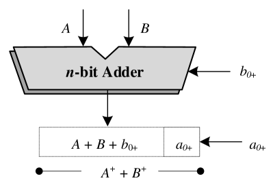
Figure 1: The addition of two $n$-bit DLSB numbers is performed using a conventional adder. The subtraction is performed with the same architecture, but with the inverted bits of $B^{+}$.

3 Design of DLSB Multiplication Circuits

In this section, we design the DLSB multiplier in two flavours, i.e., based on the straightforward approach and a more sophisticated improved approach. As baseline multiplication algorithm, we adopt the Modified Booth (MB) method [Parhami2000], which facilitates low-level optimizations and also outperforms several well-established multiplication methods [leon_IET].

1 Straightforward DLSB Design

Let $A^{+}=\langle a_{n-1}a_{n-2}\cdots a_{0}\rangle_{2\text{'s}}+a_{0+}$ and $B^{+}=\langle b_{n-1}b_{n-2}\cdots b_{0}\rangle_{2\text{'s}}+b_{0+}$ be two $n$-bit $2$’s-complement DLSB numbers. We form their product as shown in Eq. (1).

$$A^{+}\times B^{+}=\big{(}\langle a_{n-1}a_{n-2}\cdots a_{0}\rangle_{2\text{'s}}+a_{0+}\big{)}\cdot B$$ (2)

Following the Modified Booth multiplication algorithm, $B^{+}$ is encoded with its extra LSB $b_{0+}$ included in the least significant Modified Booth digit, i.e., $b_{-1}=b_{0+}$ instead of $b_{-1}=0$ (conventional encoding), as shown in Eq. (3)–(1).

$$B^{+}=-2^{n-1}b_{n-1}+{\sum}_{\begin{subarray}{c}i=0\end{subarray}}^{\begin{subarray}{c}n-2\end{subarray}}2^{i}b_{i}+b_{0+}={\sum}_{\begin{subarray}{c}j=0\end{subarray}}^{\begin{subarray}{c}n\text{/}2-1\end{subarray}}4^{j}b_{j}^{\text{\scriptsize\emph{MB}}}$$ (3)

$$\text{where }\;b_{j}^{\text{\scriptsize\emph{MB}}}=-2b_{2j+1}+b_{2j}+b_{2j-1}\;\;\implies\;\;b_{j}^{\text{\scriptsize\emph{MB}}}\in\{0,\pm 1,\pm 2$$ (4)

The Modified Booth digits $b_{j}^{\text{\scriptsize\emph{MB}}}$ $\in$ $\{0,$ ${\pm}1,$ ${\pm}2\}$ are functions of three consecutive bits of $B^{+}$ ($b_{2j+1}$, $b_{2j}$, $b_{2j-1}$), and they are formed according Table 1. Each digit is represented by three $1$-bit signals that define its sign ($s_{j}$) and absolute value ($two_{j}$, $one_{j}$). Using these encoding signals, the Modified Booth digits are calculated by Eq. (1).

$$b_{j}^{\text{\scriptsize\emph{MB}}}=(-1)^{s_{j}}\cdot(2two_{j}+one_{j}),\;\;j=0,1,\cdots n/2-$$ (5)

Using Eq. (1) and (3), the multiplication of the DLSB numbers $A^{+}$ and $B^{+}$ is formed as shown in Eq. (6).

$$A^{+}\times B^{+}=\langle a_{n-1}a_{n-2}\cdots a_{0}\rangle_{2\text{'s}}\cdot B^{+}+a_{0+}\cdot B^{+}=$$

$$=\langle a_{n-1}a_{n-2}\cdots a_{0}\rangle_{2\text{'s}}\cdot{\sum}_{\begin{subarray}{c}j=0\end{subarray}}^{\begin{subarray}{c}n\text{/}2-1\end{subarray}}4^{j}b_{j}^{\text{{\scriptsize\emph{MB}}}}+a_{0+}\cdot\big{(}\langle b_{n-1}b_{n-2}\cdots b_{0}\rangle_{2\text{'s}}+b_{0+}\big{)}$$ (6)

The implementation of the DLSB multiplier based on Eq. (6) requires a conventional Modified Booth multiplier to calculate the first term of the final expression, as well as considerable overhead to calculate the extra term $a_{0+}\cdot\big{(}\langle b_{n-1}b_{n-2}\cdots b_{0}\rangle_{2\text{'s}}+b_{0+}\big{)}$.

Table 1: Modified Booth encoding.

Input			MB Digit	Output
$b_{2j+1}$	$b_{2j}$	$b_{2j-1}$	$b_{j}^{\text{\scriptsize\emph{MB}}}$	$s_{j}$	$two_{j}$	$one_{j}$
$0$	$0$	$0$	$0$	$0$	$0$	$0$
$0$	$0$	$1$	$1$	$0$	$0$	$1$
$0$	$1$	$0$	$1$	$0$	$0$	$1$
$0$	$1$	$1$	$2$	$0$	$1$	$0$
$1$	$0$	$0$	$-2$	$1$	$1$	$0$
$1$	$0$	$1$	$-1$	$1$	$0$	$1$
$1$	$1$	$0$	$-1$	$1$	$0$	$1$
$1$	$1$	$1$	$0$	$1$	$0$	$0$

2 Sophisticated DLSB Design

To reduce the overhead derived by the calculation of the extra term in the straightforward approach, we consider an alternative representation for the operand $A^{+}$. Firstly, we examine how $A^{+}$ is formed with respect to the value of $a_{0+}$:

• if $a_{0+}=0$, we get:

  $$A^{+}=\langle a_{n-1}a_{n-2}\cdots a_{0}\rangle_{2\text{'s}}+0=\langle a_{n-1}a_{n-2}\cdots a_{0}\rangle_{2\text{'s}}$$ (7)

• if $a_{0+}=1$, and using the expression $a_{i}=-\bar{a}_{i}+1$ ($\bar{a}_{i}$: inverted $a_{i}$), we get:

  $$A^{+} = \langle a_{n-1}a_{n-2}\cdots a_{0}\rangle_{2\text{'s}}+1=-2^{n-1}a_{n-1}+{\sum}_{\begin{subarray}{c}i=0\end{subarray}}^{\begin{subarray}{c}n-2\end{subarray}}2^{i}a_{i}+1=$$ (8)

  $$=-2^{n-1}(-\bar{a}_{n-1}+1)+{\sum}_{\begin{subarray}{c}i=0\end{subarray}}^{\begin{subarray}{c}n-2\end{subarray}}2^{i}(-\bar{a}_{i}+1)+1=$$

  $$=-(-2^{n-1}\bar{a}_{n-1}+2^{n-1})-{\sum}_{\begin{subarray}{c}i=0\end{subarray}}^{\begin{subarray}{c}n-2\end{subarray}}2^{i}\bar{a}_{i}+{\sum}_{\begin{subarray}{c}i=0\end{subarray}}^{\begin{subarray}{c}n-2\end{subarray}}2^{i}+1=$$

  $$=-(-2^{n-1}\bar{a}_{n-1}+{\sum}_{\begin{subarray}{c}i=0\end{subarray}}^{\begin{subarray}{c}n-2\end{subarray}}2^{i}\bar{a}_{i})-2^{n-1}+{\sum}_{\begin{subarray}{c}i=0\end{subarray}}^{\begin{subarray}{c}n-2\end{subarray}}2^{i}+1=$$

  $$=-(-2^{n-1}\bar{a}_{n-1}+{\sum}_{\begin{subarray}{c}i=0\end{subarray}}^{\begin{subarray}{c}n-2\end{subarray}}2^{i}\bar{a}_{i})=-\langle\bar{a}_{n-1}\bar{a}_{n-2}\cdots\bar{a}_{0}\rangle_{2\text{'s}}$$

Next, we encode $A^{+}$ using the expression $a^{\prime}_{i}=a_{i}\oplus a_{0+}$. Namely, each bit of $A=\langle a_{n-1}a_{n-2}\cdots a_{0}\rangle_{2\text{'s}}$ is driven to a XOR gate along with the extra LSB $a_{0+}$ to form $A^{\prime}=\langle a^{\prime}_{n-1}a^{\prime}_{n-2}\cdots a^{\prime}_{0}\rangle_{2\text{'s}}$. Hence, $A^{+}$ is encoded as shown in Eq. (9).

$$A^{+}=(-1)^{a_{0+}}\cdot(-2^{n-1}a^{\prime}_{n-1}+{\sum}_{\begin{subarray}{c}i=0\end{subarray}}^{\begin{subarray}{c}n-2\end{subarray}}2^{i}a^{\prime}_{i})=(-1)^{a_{0+}}\cdot A^{\prime},\;\;\;\;\;\;a^{\prime}_{i}=a_{i}\oplus a_{0+}$$ (9)

This encoding is equivalent to the initial representation of $A^{+}$, as verified by assigning either $0$ or $1$ to $a_{0+}$ in Eq. (9):

• for $a_{0+}=0$, $A^{+}$ is equal to the expression of Eq. (7).

• for $a_{0+}=1$, $A^{+}$ is equal to the expression of Eq. (8).

To perform the DLSB multiplication, we use Eq. (3) for $B^{+}$ and Eq. (9) for $A^{+}$. Their product is defined as shown in Eq. (10).

$$A^{+}\times B^{+}=(-1)^{a_{0+}}\cdot A^{\prime}\cdot{\sum}_{\begin{subarray}{c}j=0\end{subarray}}^{\begin{subarray}{c}n\text{/}2-1\end{subarray}}4^{j}b_{j}^{\text{\scriptsize\emph{MB}}}=A^{\prime}\cdot{\sum}_{\begin{subarray}{c}j=0\end{subarray}}^{\begin{subarray}{c}n\text{/}2-1\end{subarray}}(-1)^{a_{0+}}\cdot 4^{j}b_{j}^{\text{\scriptsize\emph{MB}}}$$ (10)

The next step is to integrate the term $(-1)^{a_{0+}}$ in the calculation of $b_{j}^{\text{\scriptsize\emph{MB}}}$, i.e., the Modified Booth digits, which are calculated by Eq. (1). Considering that this term affects the sign (depending on the value of $a_{0+}$), we drive $s_{j}$, i.e., the sign of the Modified Booth digits, to a XOR gate along with $a_{0+}$. As a result, the absolute value of the new Modified Booth digits, labeled as $b_{j}^{\text{{\scriptsize\emph{MB}}+}}$, is the same with that of $b_{j}^{\text{{\scriptsize\emph{MB}}}}$, however, their sign depends on $s_{j}$ and $a_{0+}$. In particular, the new expression for the sign is given by Eq. (11).

$$s^{\prime}_{j}=s_{j}\oplus a_{0+}$$ (11)

Based on the above analysis, Eq. (10) is transformed to Eq. (2), and the calculation of the new Modified Booth digits is performed as shown in Eq. (2).

$$A^{+}\times B^{+}=A^{\prime}\cdot{\sum}_{\begin{subarray}{c}j=0\end{subarray}}^{\begin{subarray}{c}n\text{/}2-1\end{subarray}}4^{j}b_{j}$$ (12)

$$\text{where }\;\;b_{j}^{\text{{\scriptsize\emph{MB}}+}}=(-1)^{s^{\prime}_{j}}\cdot(2two_{j}+one_{j}$$ (13)

The logic equations of the encoding signals $s_{j}$, $one_{j}$, and $two_{j}$ are derived from Table 1. The proposed encoding circuit is illustrated in Figure 2a. Compared to the conventional Modified Booth encoder that is illustrated in Figure 2b, the proposed encoder has an extra XOR-2 gate for calculating $s^{\prime}_{j}$, which includes the extra LSB of $A^{+}$.

For the calculation of the product defined in (2), the generation of $n/2$ partial products $P\!P_{j}$ is required, as shown in Eq. (2) and (15).

$$A^{+}\times B^{+}=A^{\prime}\cdot{\sum}_{\begin{subarray}{c}j=0\end{subarray}}^{\begin{subarray}{c}n\text{/}2-1\end{subarray}}4^{j}b_{j}^{\text{{\scriptsize\emph{MB}}+}}$$ (14)

∑j=0n/2-14jP​Pj

$$\text{where }\;\;P\!P_{j}=A^{\prime}\cdot b_{j}^{\text{{\scriptsize\emph{MB}}+}}=2^{n}\,\overline{p}_{j,n}+{\sum}_{\begin{subarray}{c}i=0\end{subarray}}^{\begin{subarray}{c}n-1\end{subarray}}2^{i}p_{j,i},\;\;j=0,1,\cdots n/2-1$$ (15)

The generation of the $i$-th bit of the partial product $P\!P_{j}$ is illustrated at gate level in Figure 2c. The circuit of the DLSB partial product generator is the same with that employed in the conventional Modified Booth algorithm. To calculate the Most Significant Bit (MSB) of each partial product, we consider $a^{\prime}_{n}=a^{\prime}_{n-1}$, and thus, $a_{n}=a_{n-1}$. Their LSB is calculated considering $a^{\prime}_{-1}=0$, and thus, $a_{-1}=a_{0+}$. In comparison with the conventional Modified Booth multiplier, the generation of the partial product bits is intact, except for the LSBs, where $s^{\prime}_{j}=s_{j}\oplus a_{0+}$ is used instead of $s_{j}$.

The generated partial products are accumulated, properly weighted, using a Wallace tree [Weste2010] along with the constant terms (’$1$’s) and the correction terms ($c^{\prime}_{j}$). Finally, the carry-save output of the Wallace tree is driven to a fast prefix adder [Weste2010] to form the final result. Compared to the conventional Modified Booth multiplier, again the only difference is the use of $s^{\prime}_{j}$ instead of $s_{j}$ in the calculation of the correction terms, as shown in its logic function in Eq. (16).

$$c^{\prime}_{j}=s^{\prime}_{j}\cdot(one_{j}+two_{j})=(s_{j}\oplus a_{0+})\cdot(one_{j}+two_{j})$$ (16)

Overall, the proposed DLSB multiplier incorporates the typical stages of the Modified Booth multiplication circuit: (i) encoding, (ii) partial product generation, (iii) partial product accumulation, and (iv) final addition. As shown, with careful design and bit-level manipulations we reduce the circuit overheads of the straightforward approach: the product $a_{0+}\cdot B^{+}$ of Eq. (6) is eliminated and the only overhead regards the encoding stage, where an extra signal ($s^{\prime}_{j}$) is generated.

(a)

(b)

(c)

Figure 2: Circuits used in the DLSB multiplication: (a) DLSB Modified Booth encoder (used in the sophisticated approach), (b) conventional Modified Booth encoder (used in the straightforward approach), (c) conventional partial product generator ($a_{i}$: $i$-bit of $A$, a${}_{i}=$ $s_{j}\oplus a_{i}$, used in both approaches).

For comparison purposes, Figure 2 illustrates the partial product matrices of the $16$-bit examined multipliers, i.e., the conventional Modified Booth multiplier (Figure LABEL:fig_dtr1), the straightforward DLSB Modified Booth multiplier (Figure 3b), and the sophisticated DLSB Modified Booth multiplier (Figure 3c). All the necessary bits (partial product bits, constant terms, and correction terms) that are required for the partial product accumulation are included. As shown, the straightforward DLSB multiplier implements the conventional multiplier plus extra logic for the product $a_{0+}\cdot B^{+}$. In contrast, the sophisticated design does not implement this logic, it has the same depth of accumulation tree with the conventional multiplier, and its only difference compared to the latter is the calculation of $s^{\prime}_{j}$. This signal is used instead of $s_{j}$ for generating the LSB of the partial products ($p^{\prime}_{j,0}$) and the correction terms ($c^{\prime}_{j}$).

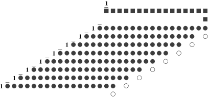
(b)

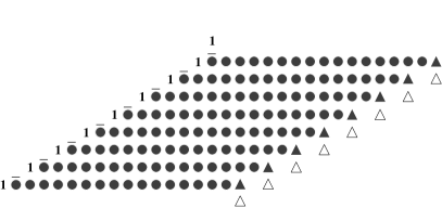
(c)

Figure 3: Partial product matrices of $16$-bit multipliers: (a) conventional Modified Booth multiplier (ordinary $2$’s-complement numbers), (b) straightforward DLSB Modified Booth multiplier of Eq. (6), (c) sophisticated DLSB Modified Booth multiplier of Eq. (2). Symbols: : $p_{j,i}$   : $c_{j}$   : $a_{0+}\cdot b_{i}$   : $p^{\prime}_{j,0}$   : $c^{\prime}_{j}$

4 Evaluation

In this section, firstly, we evaluate the DLSB multipliers, and then, we demonstrate how they can be used to improve the hardware efficiency of large-size multiplications. We conduct both theoretical and experimental analysis. We consider the following notations for the examined multipliers:

• CMB: conventional Modified Booth multiplier for ordinary $2$’s-complement numbers (Figure LABEL:fig_dtr1).

• DLSB1: straightforward Modified Booth multiplier for $2$’s-complement DLSB numbers (Figure 3b).

• DLSB2: sophisticated Modified Booth multiplier for $2$’s-complement DLSB numbers (Figure 3c).

1 Theoretical Analysis

As already discussed in the previous section, DLSB1 implements CMB and requires additional logic ($n+1$ AND-2 gates) for calculating the extra product, as well as considerable overhead for accumulating it with the rest partial products. On the other hand, DLSB2 implements CMB with a small overhead of $n/2$ XOR-2 gates for calculating $s^{\prime}_{j}$. Namely, it uses the encoder of Figure 2a instead of that of Figure 2b. Subsequently, we evaluate the area complexity of the DLSB multipliers based on the unit gate model used in [Tsoumanis2014]. According to this model, the primitive gates AND-2 and OR-2 are equal to $1$ unit gate, the NOT gate counts as $0.5$ unit gates, and the XOR-2 gate is equal to $2$ unit gates. Moreover, the area of a full adder and a half adder is $7$ and $3$ unit gates, respectively. The gate equivalence of the main components used in the partial product generation and accumulation of the multipliers is summarized in Table 2. In the next paragraphs, we examine separately the stages of the partial product generation and accumulation, and then we quantify the resources of the entire multiplication architectures.

Regarding the partial product generation, the $n$-bit CMB multiplier generates $n/2$ $(n+1)$-bit partial products, Therefore, it requires $n/2$ MB encoders of Figure 2b, $n/2$ $\!\times\!$ $(n+1)$ 1-bit partial product generators of Figure 2c, and $n/2$ correction terms generators (signals $c_{j}$). Additionally, $n/2$ NOT gates are needed for inverting the MSB of each partial product. DLSB1 requires the same resources, and also employs $n+1$ AND-2 and $1$ NOT gates for calculating the product $a_{0+}\cdot B^{+}$. Compared to CMB, DLSB2 uses only a different encoder, i.e., the DLSB encoder of Figure 2a.

Next, we analyze the resources needed for the partial product accumulation. CMB and DLSB2 accumulate $n/2+1$ $n$-bit vectors, i.e., $n/2$ partial products and $1$ vector containing the constant and correction terms. This multi-operand addition is performed in carry-save form [Weste2010], thus, $(n/2-1)$ $\times$ $n$ full adders are required in total. In DLSB1, one more number must be added, and thus, $n/2$ $\times$ $n$ full adders are required. Finally, in all multipliers, the $2n$-bit carry-save output of the Wallace tree is driven to a fast adder [Weste2010], which consists of $2n$ half adders, $n\log_{2}2n$ propagate group circuits (each one is $3$ unit gates), and $2n$ XOR-2 gates.

Based on our theoretical analysis about the resources of each design, Table 3 reports the overhead in unit gates of the DLSB multipliers for different bit-widths, i.e., $n=8,16,32$. This overhead is calculated by comparing the unit gates of the DLSB multipliers with those of CMB. As expected, DLSB1, which is based on the straightforward design approach, exhibits larger overhead compared to DLSB2. On the other hand, the overhead of DLSB2 is negligible, lying in the range $0.5\%$–$1.4\%$. The unit gate model is a simplified model, but it gives a rough estimation about the circuit area. In the next section, we provide experimental analysis based on industrial-strength synthesis of the circuits, in which it is shown that theoretical outcomes and trends follow in a fine manner the experimental results.

Table 2: Unit gates per component and components of the $n$-bit multipliers.

Component	Unit Gates	# in CMB	# in DLSB1	# in DLSB2
MB Encoder	$5.5$	$n/2$	$n/2$	–
DLSB MB Encoder	$7.5$	–	–	$n/2$
MB PP Generator	$5$	$n/2$ $\!\times\!$ $(n+1)$	$n/2$ $\!\times\!$ $(n+1)$	$n/2$ $\!\times\!$ $(n+1)$
AND PP Generator	$1$	–	$n+1$	–
Corr. Term Generator	$2$	$n/2$	$n/2$	$n/2$
Full Adder	$7$	$(n/2-1)$ $\!\times\!$ $n$	$n/2$ $\!\times\!$ $n$	$(n/2-1)$ $\!\times\!$ $n$
Half Adder	$3$	$2n$	$2n$	$2n$
Propagate Group	$3$	$n\log_{2}2n$	$n\log_{2}2n$	$n\log_{2}2n$
XOR-2 Gate	$2$	$2n$	$2n$	$2n$

Table 3: Unit gate overhead of the $n$-bit DLSB multipliers.

Multiplier	n $\mathbf{=8}$	n $\mathbf{=16}$	n $\mathbf{=32}$
DLSB1	$11.8\%$	$6.7\%$	$3.7\%$
DLSB2	$1.4\%$	$0.8\%$	$0.5\%$

2 Experimental Results

This section evaluates the multiplication circuits in terms of delay, area, and energy consumption, using industrial-strength tools. All the multipliers are implemented in Verilog and synthesized with the Synopsys Design Compiler and the TSMC 45-nm standard-cell library. The simulations are performed with Mentor Graphics QuestaSim. Both synthesis and simulation are performed at $1$V, i.e., the nominal supply voltage. Moreover, the designs are configured to operate at their critical path delay, i.e., at maximum frequency. The critical path delay and the area are reported by Synopsys Design Compiler, while the power consumption is measured with Synopsys PrimeTime. The energy consumption is also calculated by the product of delay and power.

Table 4 presents the experimental results from the synthesis of the multipliers for various sizes, i.e., $n=8,16,32$. Furthermore, the energy and area overheads compared to CMB are reported. In terms of critical paths, as expected, the DLSB multipliers deliver almost the same delays with CMB. DLSB2 exhibits similar delay even for the smallest bit-width, i.e., $0.38$ns versus $0.37$ns. This is justified by the fact that the depth of DLSB2’s partial product tree has not increased. In comparison with DLSB1, the sophisticated DLSB2 design achieves higher efficiency for all the resources. On average, DLSB2 imposes small area and energy overheads (i.e., $3.1\%$ and $3.3\%$, respectively), while the corresponding overheads for DLSB1 are $11.9\%$ and $15.4\%$. Regarding the bit-width scaling, the derived results show that as the multiplier’s size increases, the impact of the extra LSB is becoming smaller in both area and energy. This observation is normal, as by increasing the bit-width, the rate of the overheads induced by the DLSB increases slower than the rate of the area added due to the bit-width scaling.

Table 4: Synthesis results of the $n$-bit DLSB multipliers on TSMC 45-nm standard-cell.

Design		Delay	Area		Energy
		(ns)	($\upmu$m${}^{2}$)	($\%$)	($\upmu$W$\cdot$ns)	($\%$)
n $\mathbf{=8}$	CMB	$0.37$	$485$	$-$	$384$	$-$
	DLSB1	$0.40$	$572$	$+18$	$480$	$+25$
	DLSB2	$0.38$	$510$	$+5.2$	$406$	$+5.7$
n $\mathbf{=16}$	CMB	$0.51$	$1519$	$-$	$1186$	$-$
	DLSB1	$0.52$	$1701$	$+12$	$1344$	$+13.3$
	DLSB2	$0.51$	$1562$	$+2.8$	$1217$	$+2.6$
n $\mathbf{=32}$	CMB	$0.67$	$5189$	$-$	$4340$	$-$
	DLSB1	$0.67$	$5491$	$+5.8$	$4685$	$+7.9$
	DLSB2	$0.67$	$5256$	$+1.3$	$4412$	$+1.7$

• Refers to $\%$ area/energy overhead (relative increase) in comparison with CMB.

3 Case Study: DLSB for Large-Size Multiplication

In this section, we demonstrate how the sophisticated DLSB multiplier can be effectively used as building block for implementing multiplications with large input operands. For the rest of the analysis, we consider $2$’s-complement arithmetic and small fixed-size multiplication circuits, i.e., there is the constraint of hardwired arithmetic units with specific small bit-width, like in embedded devices [Dinechin2009].

We follow the well-established approach of decomposing the large bit-width operands to smaller sizes [Dinechin2009]. The reduction of the operand bit-width to match the desired bit-width (imposed by the constraint) is a recursive procedure. Nevertheless, to ease the description and without loss of generality, we focus our analysis on the first recursion, assuming that the bit-width constraint exposed by the available arithmetic unit is satisfied. Next, we discuss how the large-size multiplications are partitioned in the conventional arithmetic, and then, we present a more efficient DLSB-based partition.

Conventional $\mathbf{2}$’s-Complement Arithmetic: Let $A$ and $B$ be two $k$-bit $2$’s-complement numbers to multiply. Without loss of generality, we consider $k=2n$, where $n$ is an integer, and we split $A$ and $B$ in two $n$-bit words, as shown in Eq. (17). The product $A\times B$ is formed as shown in Eq. (18).

$$A=\langle a_{2n-1}a_{2n-2}\cdots a_{n}\rangle_{2\text{'s}}\cdot 2^{n}+\langle a_{n-1}a_{n-2}\cdots a_{0}\rangle_{\text{u}}=A_{s}\cdot 2^{n}+A$$

$$B=\langle b_{2n-1}b_{2n-2}\cdots b_{n}\rangle_{2\text{'s}}\cdot 2^{n}+\langle b_{n-1}b_{n-2}\cdots b_{0}\rangle_{\text{u}}=B_{s}\cdot 2^{n}+B_{u}$$ (17)

$$A\times B =(A_{s}\cdot 2^{n}+A_{u})\cdot(B_{s}\cdot 2^{n}+B_{u})=$$

$$=A_{s}\cdot B_{s}\cdot 2^{2n}+(A_{s}\cdot B_{u}+A_{u}\cdot B_{s})\cdot 2^{n}+A_{u}\cdot B_{u}$$ (18)

The above product requires the execution of $4$ multiplications: (i) $2$’s-complement $\times$ $2$’s-complement ($A_{s}\cdot B_{s}$), (ii) unsigned $\times$ unsigned ($A_{u}\cdot B_{u}$), (iii) unsigned $\times$ $2$’s-complement ($A_{u}\cdot B_{s}$), (iv) $2$’s-complement $\times$ unsigned ($A_{s}\cdot B_{u}$). We note that the multiplications involving unsigned numbers must employ an extra bit for the sign extension. As a result, to cover all the bit-width cases and calculate the $4$ sub-products with the same module, the $(n+1)$-bit CMB multiplier needs to be used.

$\mathbf{2}$’s-Complement DLSB Arithmetic: We propose an alternative operand partition that aims to create DLSB-like bit vectors. As shown in Eq. (19)–(20), we divide the operands in two $2$’s-complement segments, and attach the MSB of their least significant part, i.e., $a_{n-1}$ and $b_{n-1}$, as an extra LSB in their most significant part. Assuming an extra LSB equal to $0$ for the least significant parts, the $k$-bit operands are now formed as functions of two $n$-bit $2$’s-complement DLSB numbers.

$$A =\big{(}\langle a_{2n-1}a_{2n-2}\cdots a_{n}\rangle_{2\text{'s}}+a_{n-1}\big{)}\cdot 2^{n}+\big{(}\langle a_{n-1}a_{n-2}\cdots a_{0}\rangle_{2\text{'s}}+0\big{)}=$$

$$=A_{1}^{+}\cdot 2^{n}+A_{2}^{+}$$ (19)

$$B =\big{(}\langle b_{2n-1}b_{2n-2}\cdots b_{n}\rangle_{2\text{'s}}+b_{n-1}\big{)}\cdot 2^{n}+\big{(}\langle b_{n-1}b_{n-2}\cdots b_{0}\rangle_{2\text{'s}}+0\big{)}=$$

$$=B_{1}^{+}\cdot 2^{n}+B_{2}^{+}$$ (20)

Considering the proposed DLSB-based partition, the $4$ sub-products, derived by applying again the distributive property, can be calculated by the $n$-bit $2$’s-complement DLSB multiplier, which can effectively replace the $(n+1)$-bit CMB as building block. To evaluate the efficiency of the proposed scheme, we compare the $n$-bit DLSB2 with the $(n+1)$-bit CMB for various bit-widths. The experimental setup is the same as described in the previous section. Figure 4 illustrates the energy and area gains achieved by the proposed DLSB2 compared to CMB. In particular, DLSB2 provides significant gains, especially for small bit-width (i.e., $30.6\%$ and $43.3\%$ area and energy gains, respectively, for $n=8$). The inefficiency of CMB is justified by the extra bit in the multiplier’s bit-width, which results in the generation of one more partial product and the addition of an extra bit in each partial product.

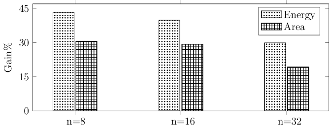
Figure 4: Energy and area gains provided by $n$-bit DLSB2 compared to $(n+1)$-bit CMB (targeting the use of DLSB2 instead of CMB as building block in large-size multiplications).

5 Conclusion

The goal of this chapter was to highlight the benefits of using novel numerical formats and applying low-level arithmetic optimizations and sophisticated bit-level manipulations. In particular, we adopted the DLSB arithmetic, which assumes an extra LSB in the number representation and provides advantageous features, such as the representation symmetry and the simplification of rounding in floating-point operations. Targeting to decrease the overheads induced by the extra LSBs, we introduced a new and effective algorithm for multiplying two $2$’s-complement DLSB numbers. Through an alternative representation, we optimized the Modified Booth multiplication scheme to decrease the overheads of the straightforward DLSB multiplication. According to our experimental evaluation for different multiplication bit-widths, our DLSB design provides average overheads of $\scriptstyle\sim$$3\%$ in area and energy. In contrast, the DLSB design that does not adopt our sophisticated low-level optimizations, suffers from average overheads of $\scriptstyle\sim$$12\%$ and $\scriptstyle\sim$$15\%$ in area and energy, respectively. Finally, we demonstrated how the proposed DLSB multiplier can be efficiently used as building block in large-size multiplications, replacing the conventional multiplier. In this case, both the area and energy consumption are significantly improved, considering that the DLSB multiplier outperforms the conventional design that is needed to implement the sub-products, by up to $30.6\%$ and $43.3\%$ in area and energy, respectively.

Chapter 5 Arithmetic Approximation: Hybrid High-Radix Encoding

Approximate Computing forms a design alternative that exploits the intrinsic error resilience of various applications and produces energy-efficient circuits with small accuracy loss. In this chapter, we examine the impact of applying low-level optimizations and disciplined approximations in the design of arithmetic circuits. Towards this direction, we propose an approximate hybrid high-radix encoding for generating the energy-efficient RAD multipliers. The proposed encoding scheme approximately encodes one of the operands, using the accurate radix-$\mathit{4}$ encoding for its most significant part and an approximate higher radix encoding for its least significant part. In the high-radix encoding, the approximations are applied by mapping all the high-radix values to a set of values that includes only the $\mathit{4}$ largest powers of two. The proposed hybrid encoding is configurable and can be tuned to achieve the desired energy–accuracy trade-off. Another important feature of the proposed design is that the error induced by the approximations is bounded by a Gaussian distribution with near-zero average. In addition, the mean relative error of the multiplication depends only on the approximately encoded operand, and thus, the calculation of the corresponding error metrics is accelerated, eliminating the need for exhaustive hardware simulations. In terms of resources, the proposed multipliers deliver up to $\mathit{56}$% energy and $\mathit{55}$% area gains compared to the accurate radix-$\mathit{4}$ multiplier, when operating at the same frequency. Moreover, our designs outperform state-of-the-art multipliers by up to $\mathit{40}$% in energy consumption for similar error values. Finally, we examine the scalability of our technique, showing that as the multiplier’s size increases, our designs achieve larger gains in energy consumption and critical path delay, i.e., up to $\mathit{64}$% and $\mathit{22}$%, respectively, while the error remains constant. This chapter is based on our publication in [LeonTVLSI].

1 Introduction

In modern embedded systems and data centers, power efficiency and performance are critical design concerns. Considering that various application domains exhibit an intrinsic error resilience (e.g., digital signal processing, data analytics, and data mining [ChakradharDAC2010, ChippaDAC2013]), Approximate Computing [2016_Mittal_ACMsrv, 2016_Xu_IEEEdt, 2021_Stanley_ACMsrv] appears as an effective solution to provide remarkable power gains and/or speed improvements. In Approximate Computing, error is viewed as a commodity that can be traded for significant gains in resources (e.g., area, power, energy, latency, or throughput) [LingamneniCICC2014], and thus, it composes a promising design paradigm to generate power-efficient systems and circuits. In particular, Approximate Computing exploits the innate error tolerance of the applications and deliberately relaxes the correctness of some computations to decrease their power consumption and/or accelerate their execution.

To take advantage of the benefits provided by Approximate Computing, massive research has been conducted in the field of approximate hardware and circuits. In this field, automated synthesis techniques [ShinDATE2010] and hardware description language annotations [2015_Yazdanbakhsh_DATE] have been proposed to facilitate the design of approximate hardware. Significant research has also been reported in approximate processors that employ quality programmable vectors [Venkataramani], neural networks [Esmaeilzadeh] and approximate custom instructions [Kamal2014]. Circuit-level approximations involve voltage over-scaling [2010_Kurdahi_IEEEtvlsi, 2017_Ragavan_DATE] and over-clocking [2015_Constantin_DATE, 2013_Shi_FCCM] techniques. Voltage over-scaling lowers the supply voltage of the circuit below the nominal value, and thus, the power consumption is decreased in exchange for erroneous outputs due to the critical paths’ failure to meet the timing constraints [2010_Kurdahi_IEEEtvlsi]. Over-clocking inserts timing violations, reducing expensive timing guard-bands and providing performance improvement [2013_Shi_FCCM]. Another approach is to apply logic-level approximations, i.e., modify the truth table, employ inexact components, or prune nodes of the circuit.

The main target of logic-level Approximate Computing is the arithmetic circuits [2020_Jiang_IEEE], which are key computation units in general-purpose processors and custom hardware accelerators. Extensive research is reported in approximate adders [GuptaTCADICS2013, 2013_Gupta_IEEEtcad, ZhuTVLSI2010, MahdianiTCSI2010, VermaDATE2008], which provide significant gains in critical path delays and power consumption. On the other hand, research activities on the approximate multipliers [KulkarniICVLSI2011, 2015_Momeni_IEEEtc, LinICCD2013, KyawEDSSC2010, LiuDATE2014, NarayanamoorthyTVLSI2015, 2015_Hashemi_ICCAD, ZervakisTVLSI2016, 2016_Jiang_IEEEtc, 2017_Liu_IEEEtc, BabicMM2011, 2017_Zendegani_IEEEtvlsi] are less comprehensive compared to the respective on approximate adders. In the multiplication circuit, approximations can be applied in the partial product generation [ZervakisTVLSI2016, 2016_Jiang_IEEEtc, 2017_Liu_IEEEtc] and the partial product accumulation [KulkarniICVLSI2011, LinICCD2013, 2015_Momeni_IEEEtc, LiuDATE2014]. Both types of approximation are synergistic and can be applied in collaboration to achieve higher power reduction [2016_Jiang_IEEEtc, 2017_Liu_IEEEtc]. Although significant research regards the partial product accumulation, approximation techniques in the partial product generation have received less attention. Another limitation of the existing approximate multipliers is that the majority of them (e.g., [2015_Momeni_IEEEtc, KulkarniICVLSI2011, KyawEDSSC2010, BabicMM2011]) does not examine signed multiplication.

In this chapter, motivated by the resource gains provided by arithmetic circuits, we present a novel hybrid high-radix encoding for approximate multipliers. Our technique addresses some of the issues of prior designs, such as the signed multiplication and the reduction of the critical paths, and it also provides better results than state-of-the-art works. The proposed encoding is hybrid, i.e., it splits the number and encodes it with two different schemes (accurate and approximate). More specifically, the Most Significant Bits (MSBs) are encoded using the accurate radix-$4$ encoding, whereas the $k$ Least Significant Bits (LSBs) are encoded using the approximate high-radix-$2^{k}$ (where $k\geq 4$). To simplify the increased complexity induced by the conventional high-radix encodings, we alter their truth tables and generate their approximate variants. Using this approximate hybrid encoding, the number of the partial products is decreased, and simpler tree architectures are used for the partial product accumulation.

The contribution of this chapter is summarized as follows:

• We highlight the efficiency of applying disciplined low-level approximations, which deliver valuable resource gains while keeping the accuracy in acceptable levels.

• We address the circuit overheads of the classic high-radix encodings, e.g., radix-$64$, radix-$256$, radix-$1024$, which constitute them inefficient for use in multiplication circuits.

• We propose a new hybrid encoding for approximate partial product generation, which is parametric in terms of approximation degree and can be combined with other techniques, e.g., with approximate partial product accumulation.

• We show that the proposed technique outperforms related state-of-the-art approximation techniques, providing remarkable area and energy gains for comparable error values.

The remainder of this chapter is organized as follows. Section 2 introduces the proposed approximate hybrid high-radix encoding and its application in the design of approximate radix-based multipliers. Section LABEL:s4_3 performs the evaluation of the proposed design, including theoretical resource analysis, error analysis, and comparative experimental results. Finally, Section LABEL:s4_4 draws the conclusions.

2 Design of Approximate High-Radix Encodings and Multipliers

Conventional high-radix operand encodings reduce the total number of partial products in multipliers, and thus, the partial product accumulation is performed with simpler adder tree architectures. However, the high-radix encoders, as well as the high-radix-based partial product generators, are characterized by increased logic complexity, negating thus the benefits of the partial product reduction. Therefore, the prevailing radix encoding for multiplication circuits is radix-$4$, outperforming its high-radix counterparts.

In this section, we propose an approximate hybrid encoding, which applies simultaneously the conventional (accurate) radix-$4$ encoding and a new (approximate) high-radix-$2^{k}$ encoding. In more detail, we present the functionality of the hybrid encoding, we introduce the proposed approximations that simplify the complexity of the conventional high-radix encoding, and finally, we design inexact multipliers based on the proposed approximate encoding.

1 Approximate Operand Encoding

Let $B$ be a $n$-bit $2$’s-complement number and $k$ be an even number belonging in the interval $[4$, $n-2]$, i.e., $k=2m\!\!:m\in\mathbb{Z}$ and $2\leq m\leq(n-2)/2$. $B$ is divided into two segments with respect to $k$: the most significant part containing its $n-k+1$ MSBs and the least significant part containing its $k$ LSBs (there is a shared bit between the two segments). The $n-k+1$ MSBs are encoded with the radix-$4$ encoding, while the $k$ LSBs are encoded with the radix-$2^{k}$ encoding, as shown in Eq. (1)–(1).

$$B=\langle b_{n-1}b_{n-2}\cdots b_{0}\rangle_{2\text{'s}}=-2^{n-1}b_{n-1}+{\sum}_{\begin{subarray}{c}i=0\end{subarray}}^{\begin{subarray}{c}n-2\end{subarray}}2^{i}b_{i}={\sum}_{\begin{subarray}{c}j=k/2\end{subarray}}^{\begin{subarray}{c}n/2-1\end{subarray}}4^{j}y_{j}^{R4}+y^{R2^{k}}$$ (1)

$$y_{j}^{R4}=-2b_{2j+1}+b_{2j}+b_{2j-1}\;\;\implies\;\;y_{j}^{R4}\in\{0,\pm 1,\pm 2$$ (2)

$$\!\!\!\!y^{R2^{k}}_{0}\!=\!-2^{k-1}b_{k-1}+2^{k-2}b_{k-2}+\dots+b_{0}\!\implies\!y^{R2^{k}}_{0}\!\!\in\!\{0,\pm 1,\dots,\pm(2^{k-1}\!\!-1),-2^{k-1}$$ (3)

Eq. (1) refers to the radix-$4$ encoded digits, while Eq. (1) refers to the radix-$2^{k}$ encoded digit. In more detail, the radix-$4$ encoding creates $(n-k)/2$ digits $y_{j}^{R4}$ $\in$ $\{0,$ $\pm 1,$ $\pm 2\}$, while the radix-$2^{k}$ encoding creates the digit $y^{R2^{k}}_{0}$ $\in$ $\{0,$ $\pm 1,$ $\pm 2,$ $\pm 3,$ $\dots,$ $\pm(2^{k-1}-1),$ $-2^{k-1}\}$. In total, $B$ is encoded with $(n-k)/2$ + $1$ digits.

The encoding circuit for the above accurate hybrid encoding features increased logic due to the large number of $y^{R2^{k}}_{0}$ values and the values that are not power of two. Therefore, we propose an alternative approximate variant of the high-radix encoding, while we keep the low-complexity radix-$4$ encoding of the MSBs to avoid huge errors. To approximate $y^{R2^{k}}_{0}$, we map all the values that are not power of two, as well as the $k-4$ smallest powers of two, to their nearest of the $4$ largest powers of two or $0$. In this way, the approximate digit $\hat{y}^{R2^{k}}_{0}$ takes values from a smaller set that includes only $4$ absolute values plus $0$. In addition, the sum of these values is $0$, like in the set of values of $y_{j}^{R4}$. We choose to keep only the $4$ largest powers of two, so that the approximate radix-$2^{k}$ encoder requires about double the logic of the $(n-k)/2$ accurate radix-$4$ encoders.

Table 1 presents the accurate radix-$4$ encoding. The signal $sign_{j}$ indicates the sign of $y_{j}^{R4}$, i.e., it is activated when the digit is negative. The signals $\times 1_{j}$ and $\times 2_{j}$ regard the magnitude of $y_{j}^{R4}$, i.e., they are activated when its magnitude is $1$ and $2$, respectively. The logic functions of these signals are provided in Eq. (4)–(6).

$$sign_{j}=b_{2j+1}$$ (4)

$$\times 1_{j}=b_{2j-1}\oplus b_{2j}$$ (5)

$$\times 2_{j}=(b_{2j+1}\oplus b_{2j})\cdot\overline{(b_{2j-1}\oplus b_{2j})}$$ (6)

Table 2 presents the approximate radix-$2^{k}$ encoding. The first two columns show the proposed mapping to create the approximate set of values ($y^{R2^{k}}_{0}\rightarrow\hat{y}^{R2^{k}}_{0}$). For example, if the value of $y^{R2^{k}}_{0}$, as originally calculated by Eq. (1), belongs in $[2^{k-5},\,2^{k-4}+2^{k-5})$, it is mapped to $2^{k-4}$. Similar to the radix-$4$ encoding, the encoding signals are activated to indicate the value of $\hat{y}^{R2^{k}}_{0}$. The logic functions of the approximate radix-$2^{k}$ encoding signals are provided in Eq. (7)–(11). We note that for $k=4$, we consider an extra bit $b_{-1}=0$.

$$sign=b_{k-1}$$ (7)

$$\times 2^{k-4}=(\overline{b}_{k-2}\cdot\overline{b}_{k-3}\cdot\overline{b}_{k-4}+b_{k-2}\cdot b_{k-3}\cdot b_{k-4})\cdot(b_{k-4}\oplus b_{k-5})$$ (8)

$$\times 2^{k-3}=\overline{b}_{k-1}\cdot\overline{b}_{k-2}\cdot(\overline{b}_{k-3}\cdot b_{k-4}\cdot b_{k-5}+b_{k-3}\cdot\overline{b}_{k-4})\;+$$

$$\hskip 37.0pt+\;b_{k-1}\cdot b_{k-2}\cdot(b_{k-3}\cdot\overline{b}_{k-4}\cdot\overline{b}_{k-5}+\overline{b}_{k-3}\cdot b_{k-4})$$ (9)

$$\times 2^{k-2}=\overline{b}_{k-2}\cdot b_{k-3}\cdot(b_{k-1}+b_{k-4})+b_{k-2}\cdot\overline{b}_{k-3}\cdot(\overline{b}_{k-1}+\overline{b}_{k-4})$$ (10)

$$\times 2^{k-1}=\overline{b}_{k-1}\cdot b_{k-2}\cdot b_{k-3}+b_{k-1}\cdot\overline{b}_{k-2}\cdot\overline{b}_{k-3}$$ (11)

Table 1: Accurate radix-$4$ encoding.

Operand Bits			R4 Digit	Encoding Signals
$b_{2j+1}$	$b_{2j}$	$b_{2j-1}$	$y_{j}^{R4}$	$sign_{j}$	$\times 2_{j}$	$\times 1_{j}$
$0$	$0$	$0$	$0$	$0$	$0$	$0$
$0$	$0$	$1$	$1$	$0$	$0$	$1$
$0$	$1$	$0$	$1$	$0$	$0$	$1$
$0$	$1$	$1$	$2$	$0$	$1$	$0$
$1$	$0$	$0$	$-2$	$1$	$1$	$0$
$1$	$0$	$1$	$-1$	$1$	$0$	$1$
$1$	$1$	$0$	$-1$	$1$	$0$	$1$
$1$	$1$	$1$	$0$	$1$	$0$	$0$

Table 2: Approximate high-radix-$2^{k}$ encoding.

Accurate Digit	Approx. Digit	Encoding Signals
$y_{0}^{R2^{k}}$	$\hat{y}^{R2^{k}}_{0}$	$sign$	$\times 2^{k-1}$	$\times 2^{k-2}$	$\times 2^{k-3}$	$\times 2^{k-4}$
$[0,\,2^{k-5})$	$0$	$0$	$0$	$0$	$0$	$0$
$[2^{k-5},\,2^{k-4}+2^{k-5})$	$2^{k-4}$	$0$	$0$	$0$	$0$	$1$
$[2^{k-4}+2^{k-5},\,2^{k-3}+2^{k-4})$	$2^{k-3}$	$0$	$0$	$0$	$1$	$0$
$[2^{k-3}+2^{k-4},\,2^{k-2}+2^{k-3})$	$2^{k-2}$	$0$	$0$	$1$	$0$	$0$
$[2^{k-2}+2^{k-3},\,2^{k-1})$	$2^{k-1}$	$0$	$1$	$0$	$0$	$0$
$[-2^{k-1},\,-2^{k-2}-2^{k-3})$	$-2^{k-1}$	$1$	$1$	$0$	$0$	$0$
$[-2^{k-2}-2^{k-3},\,-2^{k-3}-2^{k-4})$	$-2^{k-2}$	$1$	$0$	$1$	$0$	$0$
$[-2^{k-3}-2^{k-4},\,-2^{k-4}-2^{k-5})$	$-2^{k-3}$	$1$	$0$	$0$	$1$	$0$
$[-2^{k-4}-2^{k-5},\,-2^{k-5})$	$-2^{k-4}$	$1$	$0$	$0$	$0$	$1$
$[-2^{k-5},\,0)$	$0$	$1$	$0$	$0$	$0$	$0$

Overall, starting from the accurate hybrid encoding of Eq. (1)–(1), we approximate the high-radix encoding of the LSBs through the mapping of Table 2, and thus, $B$ is approximately encoded to $\tilde{B}$ as shown in Eq. (12)–(14).

$$\tilde{B}={\sum}_{\begin{subarray}{c}j=k/2\end{subarray}}^{\begin{subarray}{c}n/2-1\end{subarray}}4^{j}y_{j}^{R4}+\hat{y}^{R2^{k}}_{0}$$ (12)

$$\text{where }\;y_{j}^{R4}\in\{0,\;\pm 1,\;\pm 2\}$$ (13)

$$\text{and }\;\hat{y}^{R2^{k}}_{0}\in\{0,\;\pm 2^{k-4},\;\pm 2^{k-3},\;\pm 2^{k-2},\;\pm 2^{k-1}\}$$ (14)

Next, we present some examples to show how the proposed hybrid encoding is applied. We consider $n=16$, i.e., $16$-bit numbers and $k=6,10$, i.e., the LSBs are encoded with radix-$64$ and radix-$1024$, respectively. In the hybrid radix-$64$ encoding, the bits of $B$ are grouped as shown in Eq. (LABEL:eq_rad64b). Regarding the approximation of the radix-$64$ encoding, the $4$ largest powers of two are $\pm 4$, $\pm 8$, $\pm 16$ and $\pm 32$. Thus, we map all the rest values of the original digit $y^{R64}_{0}$ to their nearest value from the set $\{0,\;\pm 4,\;\pm 8,\;\pm 16,\;\pm 32\}$ according to Table 2 (for $k=6$).

$$\overunderbraces$$ (15)

3y6R43y4R46yR640&b15b14b13b12b11b10b9b8b7b6b5b4b3b2b1