supplemental_material

Energies and spectra of solids from the algorithmic inversion of localized $GW$

Abstract

Energy functionals of the Green’s function can provide simultaneously spectral and thermodynamic properties of interacting electrons’ systems. Exploiting a localized-GW approach, we introduce an approximation to the exchange-correlation part of the Klein functional that generalizes the energy functional of DFT+U to host a dynamical screened potential $U(\omega)$. Furthermore, we solve exactly the resulting Dyson equation extending to crystals the algorithmic-inversion method. We then compute the spectral, thermodynamic, and vibrational properties of SrVO₃, finding results in close agreement with experiments and state-of-the-art computational methods, at very reduced computational costs.

Accurate and predictive calculations of materials properties have been and remain a challenging task [1]. Though density-functional theory (DFT) has provided a major step forward in the prediction of ground-state properties [2, 3], addressing spectroscopic quantities remains challenging [4, 5, 6, 7, 8, 9]. To overcome the intrinsic limitations of DFT, dynamical methods, mostly based on Green’s functions, have been used; these includes many-body perturbation theory (MPBT) approaches such as $GW$ [10, 11], dynamical mean-field theory [12, 13] (DMFT), spectral functional theories [14, 5, 15] (SFT), and electron-boson interaction schemes [16, 17]. In all of these approaches dynamical (frequency-dependent) self-energies or potentials appear.

In Green’s function theories, the Luttinger-Ward (LW) and Klein functionals [18, 19, 20, 21, 22] are energy functionals of the Green’s function that are variational and result in conserving potentials that are dynamical. Though explicitly known diagrammatically, the exact $\Phi$ term is computationally inaccessible and needs to be approximated [23, 24]. The choice of the approximation for $\Phi$ determines the physics accessible to the functional, ranging from long-range plasmonic effects, as in $GW$ [10, 11], to strongly-correlated local interactions as in DMFT [12, 13]. The stationarity condition of the functional yields the Dyson equation involving the interacting propagator $G$ and the dynamical self-energy (as derivative of $\Phi$ wrt $G$) [21, 22]. Therefore, the functional and its derivative determine the thermodynamics and the spectral properties of a material, also allowing, at self-consistency, one to compute ground-state quantities such as forces and phonons through Hellmann-Feynman theorem  [25].

Due to the presence of dynamical quantities, applications where both spectroscopic and thermodynamic quantities are computed together are limited (see Ref. [26] and references therein). In the context of $GW$, such calculations have been performed for model systems, such as the homogeneous electron gas [27] or Hubbard chains [28], and later extended to solids, typically using an imaginary-axis formalism [29, 30, 31, 32]. This latter approach has been proven very effective for the prediction of ground-state properties, but retains limited accuracy for spectral properties, stemming from the analytic continuation to the real axis [33]. In the DMFT framework, an efficient implementation of a LW functional has made possible the calculation of ground-state quantities for crystals, while simultaneously accessing spectral properties [34, 35], notwithstanding the price of numerical limitations related to the cost of the solvers [13].

In the Letter, we adopt the Klein functional formalism to introduce a $\Phi$ term that generalizes the DFT+U energy functional of Dudarev et al. [36] to host a dynamical screened potential $U(\omega)$, rather than a static $U$. The derivative of the functional yields the localized-$GW$ self-energy of Ref. [37], together with a choice for the double-counting term. The resulting Dyson equation is treated as a non-linear eigenvalue problem, and solved via an exact mapping to a non-interacting system generalizing the “algorithmic inversion method on sum-over-poles” (AIM-SOP) [26] to the case of real materials. Within this approach, the single-particle Green’s function, along with the Dyson orbitals and excitation energies of the system, are obtained and used to calculate accurate spectral and thermodynamic properties of the material. In addition to providing an exact solution to the Dyson equation, the procedure addresses, e.g., problems with avoided crossing in the quasi-particle solution of the Dyson equation, or numerical difficulties when integrating the Green’s function to obtain thermodynamic quantities [26]. We apply this framework to the paradigmatic case study of the correlated metal SrVO₃ [38, 39, 40] finding results in very good agreement with experiments and state-of-the-art methods for the spectrum, bulk modulus, and phonons, at a greatly reduced computational cost compared to established approaches.

Algorithmic inversion method. First, we introduce a general framework to solve the Dyson equation ${G}(\omega)=[\omega I-{h}_{0}-{\Sigma}(\omega)]^{-1}$. This task can be seen as the generalization to embedded (open) systems of the diagonalization of an Hamiltonian for closed systems. Assuming $\Sigma$ to be analytical in a connected subset of the complex plane, one can exactly map the solution to the Dyson equation into the non-linear eigenvalue problem (usually shortened as NLEP [41])

$$\big{[}h_{0}+\Sigma(\omega)\big{]}\ket{\psi^{r}}=\omega\ket{\psi^{r}},$$ (1)

where $(z_{s},\psi_{s}^{r})$ are the corresponding (discrete) eigenvalues and right eigenvectors. In particular, it is possible to show that the eigenvalues $z_{s}$ are the poles of the resolvent $G(\omega)$, and, when poles are first-order (not granted in general), the right/left eigenvectors $\ket{\psi^{r}_{s}}\bra{\psi^{l}_{s}}$ provide their residues.

Though general algorithms to solve the NLEP problem exists, we consider here the self-energy to be meromorphic (isolated poles) over the whole complex plane, and to only have first-order poles. This amounts to writing the dynamical part of the self-energy (the static contribution being included in ${h}_{0}$) as a sum over poles (SOP) [42, 26]:

$${\Sigma}(\omega)=\sum_{m=1}^{N}\frac{{\Gamma}_{m}}{\omega-\Omega_{m}},$$ (2)

resulting in a truncated Lehmann representation [42]. In Eq. (2), the amplitudes ${\Gamma}_{m}$ are operators acting on the one-particle Hilbert space defined by ${h}_{0}$, and $\Omega_{m}=\omega_{m}+i\delta_{m}$ are scalars respecting the time-ordering condition $\delta_{m}\gtrless 0$ when $\Omega_{m}\gtrless\mu$, $\mu$ being the chemical potential of the system. Within these hypotheses $G(\omega)$ can also be written exactly as a SOP, and the algorithmic inversion method (AIM) allows to obtain the coefficients of the representation, as it is for the scalar homogeneous case of Ref. [26].

Introducing a factorization of the self-energy residues $\Gamma_{m}=\bar{V}^{\dagger}_{m}V_{m}$, the Green’s function reads

$${G}(\omega)=\left[\omega I-{h}_{0}-\sum_{m}\bar{V}^{\dagger}_{m}\left(\omega-\Omega_{m}\right)^{-1}V_{m}\right]^{-1}$$ (3)

which corresponds to embedding a non-interacting system ${h}_{0}$ and $N$ non-interacting fictitious degrees of freedom (baths), each having an Hamiltonian $\Omega_{i}I_{i}$ and coupled to $h_{0}$ by $\bar{V}_{i}^{\dagger},V_{i}$. Notably, the factorization of $\Gamma_{m}$ is not unique; possible choices are $V_{m}=\bar{V}^{\dagger}_{m}=\Gamma_{m}^{1/2}$ or could be based, e.g., on the singular value decomposition (SVD) of $\Gamma_{m}$. By going backwards in the embedding procedure, the total Green’s function of the system plus the baths is $G_{\text{tot}}=(\omega I_{\text{tot}}-H_{\text{AIM}})^{-1}$ with

$${H}_{\text{AIM}}=\begin{pmatrix}{h}_{0}&V_{1}&\dots&V_{N}\\ \bar{V}^{\dagger}_{1}&\Omega_{1}I_{1}&0&0\\ \vdots&0&\ddots&0\\ \bar{V}^{\dagger}_{N}&0&\dots&\Omega_{N}I_{N}\end{pmatrix};$$ (4)

in particular, $G(\omega)={P}_{0}(\omega I_{\text{tot}}-{H}_{\text{AIM}})^{-1}{P}_{0}$, with ${P}_{0}$ projecting onto the ${h}_{0}$ Hilbert space. Importantly, the freedom in the factorization of $\Gamma_{m}$ can be exploited to minimize the dimension of the subspaces corresponding to $I_{1}...I_{N}$ (i.e. making $V_{m},\bar{V}_{m}$ as rectangular as possible, e.g., via a SVD), and thereby reducing the overall dimension of the $H_{\text{AIM}}$ matrix.

At this point, while the resulting $G(\omega)$ can be expressed exactly as a SOP, it may still feature higher-order poles. This is directly connected to the question whether $H_{\text{AIM}}$ is diagonalizable (i.e. whether it admits a complete spectral representation): in the language of nonlinear eigenvalue problems, the eigenvalues of Eq. (1) need to be semi-simple [41] for the GF to have only simple poles. In turn, this depends on the nature of the self-energy. For instance, when the poles of the self-energy $\Omega_{m}$ are real (with an infinitesimal offset from the real axis), and their residues $\Gamma_{m}$ are Hermitian, the AIM matrix is Hermitian, a sufficient (but not necessary) condition for diagonalizability. In the following, the latter is assumed.

Thus, the diagonalization of $H_{\text{AIM}}$ yields the desired SOP expression for the Green’s function:

$${G}(\omega)=\sum_{s=1}^{N+1}\frac{\ket{\psi^{r}_{s}}\bra{\psi^{l}_{s}}}{\omega-z_{s}},$$ (5)

where $|\psi^{r/l}_{s}\rangle$ are the right/left eigenvectors of Eq. (1) computed, according to the above discussion, as the projections of the linear $H_{\text{AIM}}$ eigenvectors on the ${P}_{0}$ manifold, and with $z_{s}$ their eigenvalues. We have thus turned a non-linear eigenvalue problem into a linear one in a larger space. Hence, starting from the poles and residues of the self-energy this algorithmic inversion provides excitation energies, lifetimes, and amplitudes (Dyson orbitals) of the system, i.e., the real and imaginary part of the poles and their residues. Furthermore, the knowledge of the Green’s function as SOP allows for the analytic calculations of its moments and thus for the evaluation of integrated thermodynamic quantities [26]. This approach is the generalization to the non-homogeneous case of Ref. [26], in which the homogeneous electron gas was considered. Mathematically, AIM can be viewed as a special case of the “linearization” treatment of NLEP using rational functions [41]. In Ref. [43] a similar construction was used to efficiently invert the Dyson equation in the context of DMFT, with applications in Refs. [13, 44, 45]. Related approaches have also appeared recently to efficiently compute the GW self-energy and solve the Bethe-Salpeter equation [46, 47].

Localized-GW functional. Taking AIM-SOP as a formal and effective way to solve electronic-structure problems subject to dynamical potentials, here we introduce a functional formulation that generalizes the DFT+U energy functional of Dudarev et al. [36] to host a frequency-dependent screened potential $U(\omega)$. In particular, we write a localized-$GW$ Klein energy functional

$$E_{GW_{\text{Loc}}}[{G}] = E_{H}[\rho]+E_{xc}[\rho]+\Phi_{GW_{\text{Loc}}}[\mathbf{G}]$$

$$- \text{Tr}_{\omega}\left[{G}_{0}^{-1}{G}\right]+\text{Tr}_{\omega}\text{Log}\ G_{0}^{-1}G+\text{Tr}_{\omega}[h_{0}G_{0}],$$

where $\text{Tr}_{\omega}[...]$ stands for $\int\frac{d\omega}{2\pi i}e^{i\omega 0^{+}}\text{Tr}[...]$, ${G}_{0}^{-1}=\omega I-{h}_{0}$, $G$ is the Green’s function of the system, $\rho$ is the density of ${G}$, and $\mathbf{G}$ is the projection of ${G}$ onto a localized manifold of electronic states (noted as Hubbard manifold). For a single site the generalized Hubbard energy functional reads:

$$\Phi_{GW_{\text{Loc}}}[\mathbf{G}] = \frac{1}{2}\int\frac{d\omega}{2\pi i}\frac{d\omega^{\prime}}{2\pi i}\ e^{i\omega 0^{+}}e^{i\omega^{\prime}0^{+}}U(\omega^{\prime})\times$$

$$\times \Tr\{\mathbf{G}(\omega+\omega^{\prime})\left[\delta(\omega-c)\mathbf{I}-\mathbf{G}(\omega)\right]\Big{\}}$$

with $U(\omega)$ being the screened potential ${W}(\omega)$ of the system projected onto the localized space and averaged over it, and $c$ a constant aimed to address double counting.

$\Phi_{GW_{\text{Loc}}}[\mathbf{G}]$ then yields the time-ordered self-energy

$$\mathbf{\Sigma}_{GW_{\text{Loc}}}(\omega) = 2\pi i\,\frac{\delta\Phi_{GW_{\text{Loc}}}[\mathbf{G}]}{\delta\mathbf{G}}$$

$$= -\int\frac{d\omega^{\prime}}{2\pi i}e^{i\omega^{\prime}0^{+}}\,U(\omega^{\prime})\mathbf{G}(\omega+\omega^{\prime})+\frac{1}{2}U(c)\mathbf{I},$$

which is composed by the localized-$GW$ self-energy [37] (first term), and a double-counting term $\frac{1}{2}U(c)\mathbf{I}$. Here, we fix the double counting parameter $c$ as $c\to\infty$, so that $U(c)=U_{\infty}$, in agreement with Ref. [48]. Importantly, we note that $\Phi_{GW_{\text{Loc}}}$ reduces to the DFT+U Hubbard energy term of Ref. [36] when a static screened local interaction $U$ is considered. In addition, $\Phi_{GW_{\text{Loc}}}$ reduces to the $GW_{0}$ functional (plus a double-counting term) in the limit of the Hubbard manifold becoming the entire crystal. The generalization to multiple sites consists in summing different $\Phi^{I}$ terms, one per site, and is not treated here for simplicity.

Being a Klein functional with the screened interaction set to $U(\omega)$, $E_{GW_{\text{Loc}}}[{G}]$ can be made stationary by solving self-consistently the corresponding Dyson equation with a static term ${h}_{0}={h}_{\text{KS}}(\rho)$ and a self-energy

$${\Sigma}_{GW_{\text{Loc}}}(\omega)=\sum_{m,m^{\prime}}\ket{\phi_{m}}\mathbf{\Sigma}_{GW_{\text{Loc}}}^{mm^{\prime}}(\omega)\bra{\phi_{m^{\prime}}},$$ (9)

where $\{\phi_{m}\}$ span the localized Hubbard space. Here, the use of the algorithmic inversion method is crucial and provides a “closed” formulation with respect to the SOP form for the propagators. Starting with an initial Green’s function expressed on SOP, e.g., ${G}={G}_{\text{KS}}$, and a SOP for the screened interaction $U(\omega)$, the self-energy $\mathbf{\Sigma}_{GW_{\text{Loc}}}$ of Eq. (Energies and spectra of solids from the algorithmic inversion of localized $GW$), and consequently also ${\Sigma}_{GW_{\text{Loc}}}$, can be written as a SOP, since the convolution of two SOPs is a SOP [26] and the projections are just linear operations on the residues. With a self-energy on SOP, the algorithmic-inversion method can be used to find the SOP for the Green’s function. The cycle can then be iterated until self-consistency. Furthermore, the SOP form of the Green’s function naturally allows for the accurate evaluation of the generalized Hubbard energy of Eq. (Energies and spectra of solids from the algorithmic inversion of localized $GW$), the chemical potential, and in general integrated thermodynamic quantities [26].

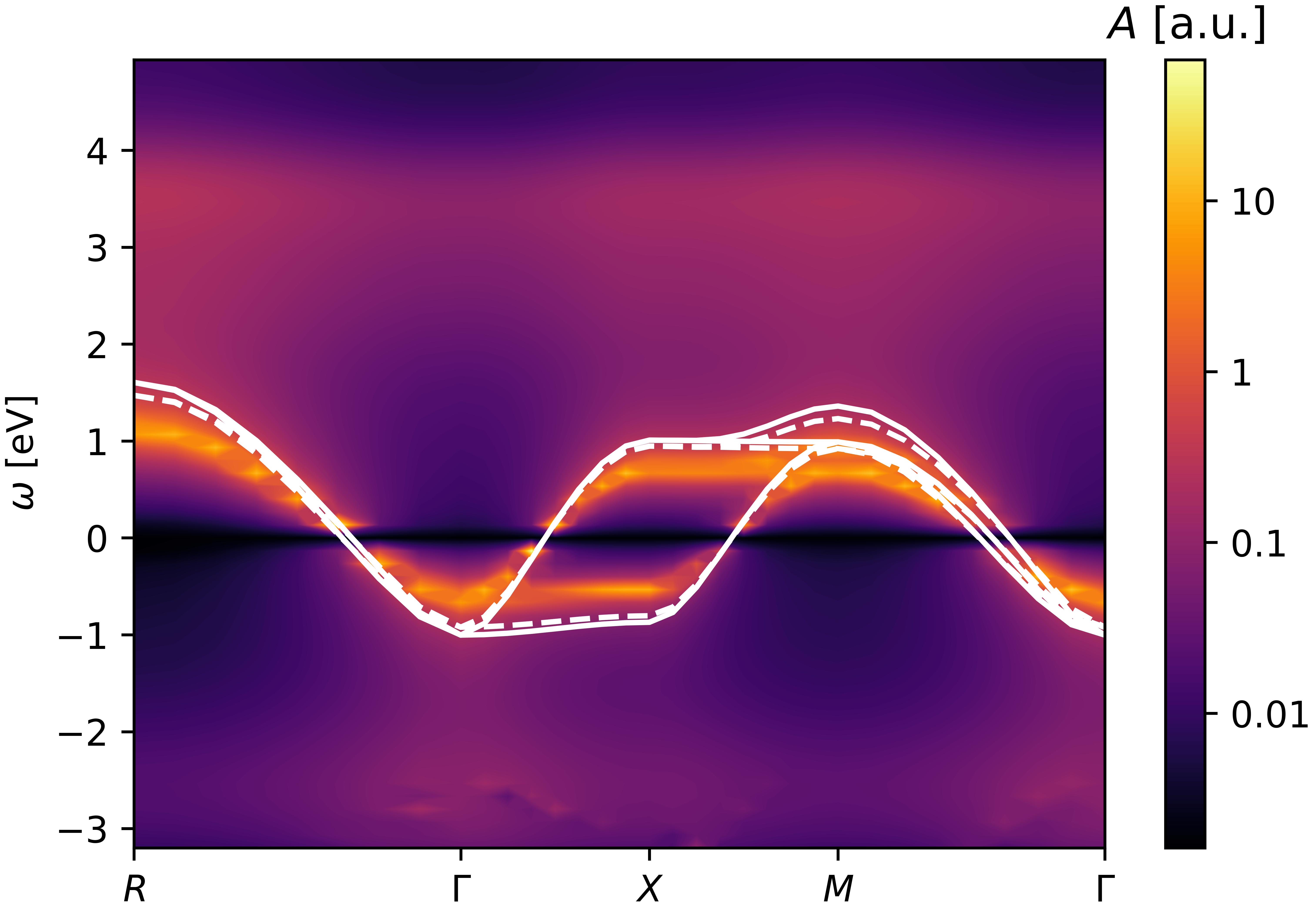
Figure 1: Spectral function of SrVO₃ from this work (color plot) compared to PBEsol (solid white line) and PBEsol+U (dashed white line). Only the t_2g bands are displayed. The chemical potential is shifted to $0$ in all three cases. The thin black band at $0$ stems from the analytic divergence of the spectral function in a metal at the chemical potential. The color map is logarithmic.

Application to SrVO₃. As a case study, we apply the formalism to the paradigmatic example of SrVO₃, where localized-$GW$ has already been proven to give qualitative good spectral results [37]. Here, we provide not only the spectral properties of the material but also integrated quantities, such as the total energy and its derivatives (lattice parameter, bulk modulus, phonons), obtained from the functional $E_{GW_{\text{Loc}}}[{G}]$. Note that in the Letter we choose a correlated metal, though the framework can be readily applied also to correlated gapped materials. As mentioned, a choice of $U(\omega)$, accounting for the dynamical screening of the electrons in the Hubbard localized manifold, is needed, and given the localized-$GW$ nature of the self-energy, and thus of the functional, we have considered $U(\omega)$ to be the average over the Hubbard space of the screened interaction $W$ in the random-phase approximation; further details are given in the Supplemental Material [49].

Though designed for self-consistency, here we limit the approach to a one-shot calculation — i.e, a single-step in the stationarization of $E_{GW_{\text{Loc}}}$ — using as starting propagator the self-consistent Kohn-Sham Green’s function computed with standard semi-local (PBEsol) DFT [50]. By doing so, we need to evaluate the energy functional at $E_{GW_{\text{Loc}}}[{G}={G}_{\text{KS}}]$, and the same for the self-energy, ${\Sigma}_{GW_{\text{Loc}}}[{G}={G}_{\text{KS}}]$. Exploiting the algorithmic-inversion method we find the non-self-consistent Green’s function. At this level, the localized-$GW$ Klein energy functional simplifies to $E_{GW_{\text{Loc}}}[{G}_{\text{KS}}]=E_{\text{DFT}}[\rho]+\Phi_{GW_{\text{Loc}}}[\mathbf{G}_{\text{KS}}]$, correcting the DFT energy with a generalized dynamical Hubbard energy term. The numerical details of the calculations are given in the Supplemental Material [49].

Method	BW	${\mathbf{m}^{*}}/{\mathbf{m}_{\text{\bf{PBEsol}}}}$	LS	US
PBEsol	$1.0$	$1$
PBEsol + U	$0.92$	$1.1$
GW+DMFT [38]	$0.5$	$2$	$-1.6$	$2$
GW+DMFT [51]	$0.6$	$2$	$-1.5$	$2.5$
GW+EDMFT [40]			$-1.7$	$2.8$
This work	$0.6$	$2$	$\begin{matrix}-1.7\\ -3.0\end{matrix}$	$\begin{matrix}2.2\\ 3.9\end{matrix}$
exp. [52]	$0.7$	$1.8$	$-1.5$
exp. [53]	$0.44$	$2$	$-1.5$

Table 1: Occupied bandwidth (BW) of the $t_{2g}$ bands, the mass enhancement factor (${{m}^{*}}/{{m}_{\text{{PBEsol}}}}$), and energy of the lower (LS) and upper satellites (US) from experiments and different theoretical frameworks. Results from the generalized dynamical Hubbard functional introduced in this work are estimated from the spectral function in Fig 1. ${{m}^{*}}/{{m}_{\text{{PBEsol}}}}$ is estimated using the ratio of the full bandwidths (LDA and PBEsol coincide). All energies are in eV.

In Fig. 1 we show the spectral function resulting from the calculations. Contrary to DFT (PBEsol), or DFT+U (PBEsol+U), that only shifts the chemical potential, the spectral function originating from $\Sigma_{GW_{\text{Loc}}}$ shows a reduction of the bandwidth along with a renormalization of the full width of the t_2g bands. In Tab. 1 we report the bandwidth (BW), the mass enhancement factor (${{m}^{*}}/{{m}_{\text{{PBEsol}}}}$), and the positions of the lower/upper satellites (LS/US). While PBEsol and PBEsol+U overestimate occupied and full bandwidth, the present results reproduce the data of Ref. [37] from localized-$GW$ and are in very good agreement with experiments [52, 53] and DMFT [51, 40, 38].

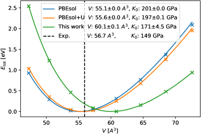
Figure 2: Equation of state for SrVO₃ calculated using PBEsol (blue), PBEsol+U (orange), and the present approach (green). Data (crosses) are fitted using the Birch-Murnaghan curve (in solid). The values and errors obtained using the fit are displayed in the legend. For reference, in dashed black we mark the experimental volume, and report the bulk modulus in the legend. Experimental values are taken from [54].

From the knowledge of the SOP of the Green’s function (here KS) and the functional form of $\Phi_{GW_{\text{Loc}}}$, we can straightforwardly calculate total energies and total-energy differences. In Fig. 2 we compare the equation of state for SrVO₃ as obtained from PBEsol, PBEsol+U, and the present dynamical formulation. In the legend we report the estimated values for the equilibrium volume $V$ and the bulk modulus $B$, using a Birch-Murnagan third-order function for the fitting [55]. It can be observed that the present approach correctly predicts the softening of the bulk modulus, while over correcting the equilibrium lattice parameter, which can be attributed to the lack of self consistency in the calculations. In the Supplemental Material [49] we analize the softening of the bulk modulus in terms of charge rearrangement.

(THz)	PBEsol	LDA+EDMFT [35]	This work
$\omega_{1}$	4.86	4.3	3.9
$\omega_{2}$	10.3	9.0	9.4
$\omega_{3}$	11.0	11.2	12.1
$\omega_{4}$	17.3	18.9	19.4

Table 2: Zone center phonons for SrVO₃ calculated with different approaches; the last column shows the results obtained using the generalized dynamical functional introduced in this work (on top of PBEsol). The data from Ref. [35] have been estimated from the plot.

Finally, using the relaxed structures, and taking advantage of the inexpensive computational cost of the present method, we report in Tab. 2 the zone-center phonons for SrVO₃. Since the Hellmann-Feynman theorem does not apply due to the lack of self-consistency, we evaluate the forces for the different displacements of the atoms with finite total energy differences. In line with the softening of the bulk modulus, the first two frequencies are lowered wrt PBEsol calculations. Also, similarly to state-of-the-art methods such as LDA+EDMFT [35] the remaining optical modes are shifted higher in frequency.

In conclusion, in the Letter we provide a computationally straightforward Green’s function framework to address the electronic structure in correlated materials using dynamical potentials. First, we link the solution of Dyson-like equations to non-linear eigenvalue problems, and solve them extending the algorithmic inversion method on sum over poles (AIM-SOP) of Ref. [26] to realistic materials. Then, we present an approximation to the exchange-correlation $\Phi$ part of the energy Klein functional, yielding a localized-$GW$ self-energy, and providing a dynamical generalization of DFT+U. Though not aiming to treat strong correlations, we combine this functional with the algorithmic-inversion method to study the paradigmatic case of SrVO₃, showing results that are close to state-of-the-art computational approaches, but with a modest computational cost, and accessing simultaneously spectral and thermodynamic properties (total energies and differences). Moreover, the existence of a Klein functional guarantees the possibility to perform self-consistent calculations, and thus to use the Hellmann-Feynman theorem to calculate forces in a Green’s function formalism. Further refinements of the dynamical functional can also be investigated.

We acknowledge stimulating discussions with Mario Caserta and Marco Vanzini. This work was supported by the Swiss National Science Foundation (SNSF) through grant No. 200021-179138 (T.C.) and NCCR MARVEL (N.M.), a National Centre of Competence in Research through grant No. 205602, and from the EU Commission for the MaX Centre of Excellence on ‘Materials Design at the eXascale’ under grant No. 101093374 (A.F., N.M.).

References

- Marzari et al. [2021] N. Marzari, A. Ferretti, and C. Wolverton, Nature Materials 20, 736 (2021).
- Hohenberg and Kohn [1964] P. Hohenberg and W. Kohn, Physical Review 136, B864 (1964).
- Kohn and Sham [1965] W. Kohn and L. J. Sham, Physical Review 140, A1133 (1965).
- Borghi et al. [2014] G. Borghi, A. Ferretti, N. L. Nguyen, I. Dabo, and N. Marzari, Physical Review B 90, 075135 (2014).
- Ferretti et al. [2014] A. Ferretti, I. Dabo, M. Cococcioni, and N. Marzari, Physical Review B 89, 195134 (2014).
- Perdew et al. [2017] J. P. Perdew, W. Yang, K. Burke, Z. Yang, E. K. U. Gross, M. Scheffler, G. E. Scuseria, T. M. Henderson, I. Y. Zhang, A. Ruzsinszky, H. Peng, J. Sun, E. Trushin, and A. Görling, Proceedings of the National Academy of Sciences 114, 2801 (2017).
- Nguyen et al. [2018] N. L. Nguyen, N. Colonna, A. Ferretti, and N. Marzari, Physical Review X 8, 021051 (2018).
- De Gennaro et al. [2022] R. De Gennaro, N. Colonna, E. Linscott, and N. Marzari, Physical Review B 106, 035106 (2022).
- Colonna et al. [2022] N. Colonna, R. De Gennaro, E. Linscott, and N. Marzari, Journal of Chemical Theory and Computation 18, 5435 (2022).
- Hedin and Lundqvist [1970] L. Hedin and S. Lundqvist, in Solid State Physics, Vol. 23, edited by F. Seitz, D. Turnbull, and H. Ehrenreich (Academic Press, 1970) pp. 1–181.
- Reining [2018] L. Reining, Wiley Interdisciplinary Reviews: Computational Molecular Science 8, e1344 (2018).
- Georges et al. [1996] A. Georges, G. Kotliar, W. Krauth, and M. J. Rozenberg, Reviews of Modern Physics 68, 13 (1996).
- Kotliar et al. [2006] G. Kotliar, S. Y. Savrasov, K. Haule, V. S. Oudovenko, O. Parcollet, and C. A. Marianetti, Reviews of Modern Physics 78, 865 (2006).
- Savrasov and Kotliar [2004] S. Y. Savrasov and G. Kotliar, Physical Review B 69, 245101 (2004).
- Vanzini et al. [2022] M. Vanzini, A. Aouina, M. Panholzer, M. Gatti, and L. Reining, npj Computational Materials 8, 1 (2022).
- Caruso et al. [2018] F. Caruso, C. Verdi, S. Poncé, and F. Giustino, Physical Review B 97, 165113 (2018).
- Zhou et al. [2020] J. S. Zhou, L. Reining, A. Nicolaou, A. Bendounan, K. Ruotsalainen, M. Vanzini, J. J. Kas, J. J. Rehr, M. Muntwiler, V. N. Strocov, F. Sirotti, and M. Gatti, Proceedings of the National Academy of Sciences 117, 28596 (2020).
- Luttinger and Ward [1960] J. M. Luttinger and J. C. Ward, Physical Review 118, 1417 (1960).
- Baym and Kadanoff [1961] G. Baym and L. P. Kadanoff, Physical Review 124, 287 (1961).
- Baym [1962] G. Baym, Physical Review 127, 1391 (1962).
- Martin et al. [2016] R. M. Martin, L. Reining, and D. M. Ceperley, Interacting Electrons: Theory and Computational Approaches (2016).
- Stefanucci and Leeuwen [2013] G. Stefanucci and R. v. Leeuwen, Nonequilibrium Many-Body Theory of Quantum Systems: A Modern Introduction (2013).
- Almbladh et al. [1999] C.-O. Almbladh, U. V. Barth, and R. V. Leeuwen, International Journal of Modern Physics B 13, 535 (1999).
- Dahlen and Barth [2004] N. E. Dahlen and U. v. Barth, Physical Review B 69, 195102 (2004).
- Haule and Pascut [2016] K. Haule and G. L. Pascut, Physical Review B 94, 195146 (2016).
- Chiarotti et al. [2022] T. Chiarotti, N. Marzari, and A. Ferretti, Physical Review Research 4, 013242 (2022).
- Holm and von Barth [1998] B. Holm and U. von Barth, Physical Review B 57, 2108 (1998).
- Honet et al. [2022] A. Honet, L. Henrard, and V. Meunier, AIP Advances 12, 035238 (2022).
- Kutepov et al. [2009] A. Kutepov, S. Y. Savrasov, and G. Kotliar, Physical Review B 80, 041103 (2009).
- Kutepov et al. [2012] A. Kutepov, K. Haule, S. Y. Savrasov, and G. Kotliar, Physical Review B 85, 155129 (2012).
- Grumet et al. [2018] M. Grumet, P. Liu, M. Kaltak, J. c. v. Klimeš, and G. Kresse, Phys. Rev. B 98, 155143 (2018).
- Yeh et al. [2022] C.-N. Yeh, S. Iskakov, D. Zgid, and E. Gull, Physical Review B 106, 235104 (2022).
- Kutepov and Kotliar [2017] A. L. Kutepov and G. Kotliar, Physical Review B 96, 035108 (2017).
- Haule and Birol [2015] K. Haule and T. Birol, Physical Review Letters 115, 256402 (2015).
- Koçer et al. [2020] C. P. Koçer, K. Haule, G. L. Pascut, and B. Monserrat, Physical Review B 102, 245104 (2020).
- Dudarev et al. [1998] S. L. Dudarev, G. A. Botton, S. Y. Savrasov, C. J. Humphreys, and A. P. Sutton, Physical Review B 57, 1505 (1998).
- Miyake et al. [2013] T. Miyake, C. Martins, R. Sakuma, and F. Aryasetiawan, Physical Review B 87, 115110 (2013).
- Tomczak et al. [2014] J. M. Tomczak, M. Casula, T. Miyake, and S. Biermann, Physical Review B 90, 165138 (2014).
- Sakuma et al. [2014] R. Sakuma, C. Martins, T. Miyake, and F. Aryasetiawan, Physical Review B 89, 235119 (2014).
- Boehnke et al. [2016] L. Boehnke, F. Nilsson, F. Aryasetiawan, and P. Werner, Physical Review B 94, 201106 (2016).
- Güttel and Tisseur [2017] S. Güttel and F. Tisseur, Acta Numerica 26, 1 (2017).
- Engel et al. [1991] G. E. Engel, B. Farid, C. M. M. Nex, and N. H. March, Physical Review B 44, 13356 (1991).
- Savrasov et al. [2006] S. Y. Savrasov, K. Haule, and G. Kotliar, Physical Review Letters 96, 036404 (2006).
- Wang et al. [2012] L. Wang, H. Jiang, X. Dai, and X. C. Xie, Physical Review B 85, 235135 (2012).
- Budich et al. [2012] J. C. Budich, R. Thomale, G. Li, M. Laubach, and S.-C. Zhang, Physical Review B 86, 201407 (2012).
- Bintrim and Berkelbach [2021] S. J. Bintrim and T. C. Berkelbach, The Journal of Chemical Physics 154, 041101 (2021).
- Cho et al. [2022] Y. Cho, S. J. Bintrim, and T. C. Berkelbach, Journal of Chemical Theory and Computation 18, 3438 (2022).
- Vanzini and Marzari [2023] M. Vanzini and N. Marzari, in preparation (2023).
- [49] See Supplemental Material for computational details and further discussion of the theoretical approach adopted.
- Perdew et al. [1996] J. P. Perdew, K. Burke, and M. Ernzerhof, Physical Review Letters 77, 3865 (1996).
- Sakuma et al. [2013] R. Sakuma, P. Werner, and F. Aryasetiawan, Physical Review B 88, 235110 (2013).
- Yoshida et al. [2005] T. Yoshida, K. Tanaka, H. Yagi, A. Ino, H. Eisaki, A. Fujimori, and Z.-X. Shen, Physical Review Letters 95, 146404 (2005).
- Takizawa et al. [2009] M. Takizawa, M. Minohara, H. Kumigashira, D. Toyota, M. Oshima, H. Wadati, T. Yoshida, A. Fujimori, M. Lippmaa, M. Kawasaki, H. Koinuma, G. Sordi, and M. Rozenberg, Physical Review B 80, 235104 (2009).
- Maekawa et al. [2006] T. Maekawa, K. Kurosaki, and S. Yamanaka, Journal of Alloys and Compounds 426, 46 (2006).
- Birch [1947] F. Birch, Physical Review 71, 809 (1947).