A Scalable Space-efficient In-database Interpretability Framework for Embedding-based Semantic SQL Queries

Abstract.

AI-Powered database (AI-DB) is a novel relational database system that uses a self-supervised neural network, database embedding, to enable semantic SQL queries on relational tables. In this paper, we describe an architecture and implementation of in-database interpretability infrastructure designed to provide simple, transparent, and relatable insights into ranked results of semantic SQL queries supported by AI-DB. We introduce a new co-occurrence based interpretability approach to capture relationships between relational entities and describe a space-efficient probabilistic Sketch implementation to store and process co-occurrence counts. Our approach provides both query-agnostic (global) and query-specific (local) interpretabilities. Experimental evaluation demonstrate that our in-database probabilistic approach provides the same interpretability quality as the precise space-inefficient approach, while providing scalable and space efficient runtime behavior (upto 8X space savings), without any user intervention.

1. Introduction

AI-Powered Database (AI-DB) is a novel approach for enabling semantic capabilities in relational databases by using a built-in self-supervised neural network model (Bordawekar and Shmueli, 2016, 2017; Bordawekar, 2018). AI-DB is built on an observation that there is a large amount of untapped hidden information in a database relation, mainly in the form of inter-/intra-column, and inter-row relationships. Further, current SQL queries, various text extensions, and user-defined functions (UDFs) are not sufficient to retrieve this information. AI-DB employs a self-supervised neural network called, database embedding (db2Vec), to capture this latent information from relational tables (Bordawekar and Shmueli, 2017). For a relational table, db2Vec builds a semantic model that captures inter- and intra-column relationships between entities of different types (db2Vec is governed by the relational data model (Date, 1982), not by a language model). After training, AI-DB seamlessly integrates the trained model into the existing SQL query processing infrastructure and uses it to enable a new class of SQL-based semantic queries called Cognitive Intelligence (CI) queries. The CI queries use the trained embedding vectors to extend the traditional value-based SQL query capabilities of the relational data model to enable semantic operations on relational entities. The output of a SQL CI query is a ranked list of rows that is ordered by a relevance similarity score. Both Spark (Bordawekar, 2018) and native Python implementations of AI-DB support a variety of CI queries, including similarity, dissimilarity, and inductive reasoning queries such as analogies or semantic clustering, and semantic grouping (Neves et al., 2019). The recently released IBM^® Db2^® 13 for z/OS^® SQL Data Insights (IBM Db2 13 Project Team, 2022) is an implementation of AI-DB in Db2^® 13 for z/OS^® on the IBM zSystems^® platform (IBM, 2022).

Given that the semantic operations are based on the meanings inferred during the database embedding training process, it is imperative that the end user understands the dominant factors that impact the result rankings. Describing result rankings in terms of just database embeddings can be opaque and inscrutable to a customer. The main goal of this work is to provide simple, transparent, and relatable result insights that are accessible to traditional database users, who may not be familiar with the intricacies of machine learning (ML) approaches. The key to understanding how the database embedding works is to get details on the co-occurrence statistics of the input data and expose their influence of the result rankings. Since any relational table has a large number of entities of different types, it is not a trivial task to explore such a large amount of statistical information.

This paper describes the design and implementation of a scalable, space-optimized intepretability infrastructure in AI-DB (Figure 1). Key novelties from our work include:

• A new approach that enables both query-agnostic (global) and query-specific (local) interpretability for the self-supervised database embedding model, db2Vec.

• Support for interpreting ranked results from a semantic similarity function by identifying dominant entities from the input relational table

• Implementing hooks in the db2Vec code to extract model-intrinsic token occurrence statistics.

• Introduction of two numeric metrics, Influence and Discriminator scores, to enable local model interpretability as well as capturing input data characteristics

• Using a probabilistic in-memory data structure, Count-Min sketch, to store the co-occurrence counts, followed by using a sparse matrix storage format to generate its serialized representation, and then populating an auxiliary relational table to be used at runtime for global function interpretability.

• Integration of the interpretability capability into the end-to-end AI-DB pipeline.

Although the co-occurrence based interpretabilty has been currently designed for AI-DB, it has broader applicability for understanding results from querying any context-based vector embedding models such as Large Language Models (LLMs) designed for different domains such as text, chemistry, or coding (Nvidia, 2023; Face, 2023; Neelakantan et al., 2022).

The rest of the paper is organized as follows. Section 2 describes the notion of interpretability, and discusses recent related work. Section 3 first presents an overview of AI-Powered Database and semantic SQL CI queries and then discusses how interpretability is used for providing insights into AI-DB’s SQL CI queries. Section 4 introduces two intepretability approaches and details implementation of a space-efficient data structure based on the Count-Min sketch. Section 5 presents experimental evaluation of the sketch data structure and its usage in interpreting AI-DB semantic operations. Finally we conclude in Section 6.

2. Related Work

Understanding the entire lifecycle of machine learning or deep learning usage, from preparing the training data, setting up the training instance, and then using the trained model to get results, is a very active area of investigation towards creating responsible AI. The main goal of these activities is provide users with different ways to understand, assimilate, and develop trust in the results generated by the trained AI model.

A majority of current explorations towards understanding the behavior of an AI model are targeted towards supervised models designed to predict a target class for an unseen value (classification). In literature, such work on understanding AI models is often referred to as interpretability or explainability (Molnar, 2022; Arrieta et al., 2019; Danilevsky et al., 2020; Gilpin et al., 2018; Marcinkevics and Vogt, 2020). Typically, explainability refers to techniques that aim to provide insights into results from a black box model via creating a second post hoc model (Rudin, 2019), whereas interpretability refers to white box techniques that use model-intrinsic information to provide result insights. These techniques can be further characterized by the scope of their inquiries: global approaches provide query-agnostic insights on the overall structure, parameters, and behavior of a model, whereas local approaches help understand how a model makes decisions for an individual prediction query (Du et al., 2020).

Traditional machine learning (ML) models such as generalized linear models (GLMs), decision trees, or tree-based ensemble models use feature engineering to map raw data into features. In contrast, deep learning (DL) models, such as the embedding models used in this work, learn representations from raw data. In the case of ML models, one can use a measure called feature importance to capture the statistical contribution of each feature into the overall decision making process to enable global interpretability. For simple ML approaches such as GLM or decision trees, it is often very easy to capture feature importance. However, for tree-based ensemble models (e.g., random forests or gradient boosted machines such as XGBoost or LightGBM), different techniques, e.g., feature coverage, are needed to capture the contributions of each individual feature (Du et al., 2020). Other examples of global interpretability include exploiting algorithmic internal information such as distribution plots, dependence plots which showcase the marginals and their interactions, permutation feature importance which perturb values and measure error to rank features.

Examples of query-specific local explanation tools include LIME (Local Interpretable Model-Agnostic Explanations) (Ribeiro et al., 2016) and SHAP (SHapley Additive exPanations) (Lundberg and Lee, 2017). LIME is a model-agnostic technique that, for any individual prediction query, approximates behavior of a black-box ML or DL model by using an interpretable surrogate model (e.g., a decision tree or a linear classifier with strong regularization). The outputs (predictions) of the surrogate model using a permuted sample input data are then computed. These predictions along with the information on the data permutations, provide insights on the contributions of each feature on the prediction of a data sample. SHAP is a game theory-based model agnostic local interpretability method, which provides how every feature contributes to the prediction, assuming each feature or group of features is a player in game theory context. The SHAP algorithm returns a Shapley value that expresses model prediction as a linear combination of binary variables that describe if a particular feature is present in the model or not. Both LIME and SHAP approaches work for multiple types of supervised ML and DL models.

Unlike supervised learning, understanding results from unsupervised or self-supervised DL models (e.g., vector embedding models) has not received enough attention. Traditional approaches such as LIME or SHAP are not able to explain vector embedding models due to the complex internal representations learned from the raw data (Ho, 2022). Recently there have been a few post hoc local explainability proposals (Madsen et al., 2021) to understand the embedding model: approaches such as SPINE (Subramanian et al., 2017) and others (Zhang et al., 2019, 2020) rely either on supplementing the embedding process by another network architecture or create new embeddings using the existing embeddings as input, while  (Celli, 2021) tries to explain the word embedding model by exploiting external lexical resources. Allen et al. (Allen and Hospedales, 2019) explains analogy queries on a word embedding model using Pointwise Mutual Information (Church and Hanks, 1990). Structural probing covers a class of methods that use an external classifier (e.g., a logistic regression) to learn a mapping from an internal representation to a linguistic representation, e.g., BERTology (Belinkov and Glass, 2018; Rogers et al., 2020; Madsen et al., 2021). Unlike the local explanation approaches, global post hoc explanation approaches aim to describe the entire model in form of relationships between the words in the vocabulary. Usually such methods employ transformations over the embedding matrix such as projections to two or three dimensions, e.g., PCA (Karl Pearson, 1901) or t-SNE (van der Maaten and Hinton, 2008), or rotation (Park et al., 2017). Recently, the topic of whether the attention mechanism (Bahdanau et al., 2014) used in the transformer models (Vaswani et al., 2017) is suited for explaination  (Jain and Wallace, 2019; Wiegreffe and Pinter, 2019) has been debated (Bibal et al., 2022) and has shown promise for some domains of application such as translation.

Overall, for self-supervised DL models, currently most approaches are post hoc, focusing on different aspects of the trained model. Currently, there is no single post hoc approach or an interpretability approach that uses model-intrisic information for providing detailed insights into the behavior of various self-supervised DL models. None of these techniques apply for the AI-DB scenario as the underlying model (db2Vec) is a specialized self-supervised DL model, built over a relational table with text and numeric entities (i.e., the training is governed by the relational data model, not a language model), and the result is a list of ranked rows, not a value to be predicted.

3. AI-Powered Database Overview

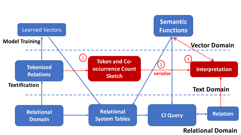
Figure 1. AI-Powered Database (AI-DB) execution stages. Operations are executed in three domains: relational, text, and vector.

Figure 1 presents key stages in the execution flow of an AI-Powered Database (Figure 1). The first preprocessing phase takes a relational table with different SQL types as input and returns an unstructured but meaningful text corpus consisting of a set of English-like sentences. This transformation, termed textification, allows us to generate a uniform semantic representation of different SQL types. The textification phase processes each relational row separately and for each row, converts data of different SQL data types to equivalent text representation (tokens). For example, numeric values are first clustered (Bordawekar and Shmueli, 2016), and then each numeric value is replaced by a string token that represents the corresponding numeric cluster (e.g., a value 121 is represented by a token c3, if 121 is mapped to the cluster 3.)

Once a relational table is converted into a textual training dataset, it is processed by a self-supervised neural network, database embedding (db2Vec), to generate semantic vectors for every unique entity in the training dataset (training phase) (Bordawekar and Shmueli, 2016, 2017). The db2Vec differs from other NLP vector embedding models used for language modeling, such as Word2Vec (Mikolov et al., 2013) or GloVe (Pennington et al., 2014) in several ways. Key differences include:

• A sentence generated from a relational row is not in any natural language such as English. In the db2Vec implementation, every token in the training set has the same influence on the nearby tokens; i.e. the generated sentence is viewed as an unordered bag of words, rather than an ordered sequence.

• Unlike the untyped text document being used in NLP, the tokens in the textified training document are typed as per the associated column name in the relational table.

• db2Vec builds a common vector-embedding model over a multi-modal relational table that can contain entities of different types such as numeric values. The trained vectors are untyped, thus enabling semantic operations on relational values of different types.

• For relational data, db2Vec provides special consideration to primary keys. Traditional word embedding approaches discard less frequent words from computations. In our implementation, by default, every token, irrespective of its frequency, is assigned a vector. For an unique primary key, its vector represents the meaning of the entire row.

• The db2Vec model provides special treatment for the entities corresponding to the SQL NULL (or equivalent) values. The NULL values are processed such that they do not contribute to the meanings of neighboring non-null entities; thus eliminating false similarities.

For each database value in a relational table, the model generates a meaning vector that encodes contextual semantic relationships generated by collective contributions of other tokens within and across rows (each table row is viewed as a sentence). The db2Vec model generates a variety of semantic vectors: (1) each unique primary key is associated with a semantic vector that captures behavior of the entire relational row associated with that key, (2) for all other entities, their semantic vectors capture collective contributions of their neighborhood entities across their occurrences, and (3) table schema types (column names) get their meaning vectors that capture table-wide relationships. Once the model is trained, the model storage phase stores the model into a relational systems table using a token as the key, and the corresponding meaning vector as the value.

The final query execution phase is where the user issues SQL statements to extract information from one or more databases using the trained db2Vec models. Such queries, termed Cognitive Intelligent (CI) queries, can support both the traditional value-based as well as the new semantic contextual computations in the same query (Bordawekar and Shmueli, 2017; Neves et al., 2019). Each CI query uses special semantic functions to measure semantic similarity between tokens associated with the input relational parameters. The core computational operation of a semantic function is to calculate similarity between a pair of tokens by computing the cosine distance between the corresponding meaning vectors. For two vectors $v_{1}$ and $v_{2}$, the cosine distance is computed as $cos(v_{1},v_{2})=cos(v_{1},v_{2})=\frac{v_{1}\cdot v_{2}}{\lVert{v_{1}}\rVert\lVert{v_{2}}\rVert}$. The cosine distance value varies from 1.0 (very similar) to -1.0 (very dissimilar).

 

SELECT C.CUSTOMER_NAME, AI_SIMILARITY(C.CUSTOMER_NAME,’CUST0’)

AS similarityValue

FROM Customer_View C

WHERE AI_SIMILARITY(C.CUSTOMER_NAME, ‘CUST0’) > 0.5

ORDER BY similarityValue DESC

 

Figure 2. Example of a SQL CI similarity query: find customers with similar overall behavior as other customers

Figure 2 presents a simple CI SQL query that given a customer identifier, CUST0, identifies other customers with the similar overall behavior (each row in the view Customer_View represents a customer transaction). The semantic function, AI_SIMILARITY(), takes relational variables as input, and returns a similarity score computed via invoking cosine similarity over corresponding meaning vectors. The SQL CI query then returns those rows whose semantic similarity is higher than a specified bound (0.5), ranked in a decreasing order of the similarity value. Customers whose similarity scores are closer to 1.0, are viewed to be semantically similar to the input customer, CUST0. Irrespective of the SQL data types of input parameters, the similarity computations are executed using untyped meaning vectors. This enables CI queries to invoke semantic functions on parameters of different SQL data types. Thus, unlike the supervised training model that works only for the target entity it was trained for, a single database embedding model can be used for answering semantic queries over a value of any SQL data type from the associated relational table.

3.1. Interpretability in AI-DB

Unlike the vector embedding models used in NLP, db2Vec trains an input training document using the relational data model (Date, 1982). db2Vec operates on a training document which is an untyped textified version of a relational table, and views it as a set of neighborhood contexts, each defined by the corresponding row in the input relational source. Each context is viewed as an unordered bag of words, where each token is equally related to other tokens in the context (in contrast, NLP vector embedding techniques view a training document as a sequence of words whose relationship is inversely proportional to the distance between the words).

Each textified token is represented as a tuple, type:value, where type denotes the corresponding column name, and value represents the textified representation of the associated relational entity. From a training perspective, db2Vec separates input tokens in three groups: (1) primary-key tokens, (2) empty (EMT) tokens corresponding to the SQL NULL values, (3) all other tokens (Figure 3). For those tokens representing unique primary key values, their inferred meaning is generated using contributions from internal tokens only within its neighborhood (i.e., corresponding row in the relational source). The primary key token does not contribute to the meaning of any other tokens in the training document (Figure 3(a)). All empty tokens corresponding to SQL NULL values (e.g., cl4:EMT, Figure 3(b)) are neglected during training (i.e., no vectors are generated). For the remaining internal tokens, within a neighborhood, each internal token contributes to the meaning of other internal tokens and vice versa (Figure 3(c)). An internal token can appear multiple times in a training document (e.g., cl1:a1, represents a relational value occurring in multiple row); its final inferred meaning is the collective contributions of all other internal tokens that co-occur in multiple contexts (Figure 3(d)).

Using aforementioned rules, db2Vec traverses the training document multiple times, iteratively building the semantic model. As the training progresses, each token becomes related to every other token in the training document, even if the tokens do not co-occur. This can impact the relationships between co-occurring tokens; for example, in Figure 3(e), although the token cl1:a1 has the same co-occurrence count of 2 with tokens cl5:e1 and cl5:e3, cl1:a1 is more closely related to cl5:e1, as they share the two neighbors, cl2:b1, and cl3:c1, with the same co-occurrence count as cl1:a1 and cl5:e1. Thus, the primary relationship between cl1:a1 and cl5:e1 gets strengthened by the secondary relationships of the shared neighbors. At the end of training, db2Vec generates a semantic model containing real-valued vectors of dimension, $d=320$, for every unique token in the input training document.

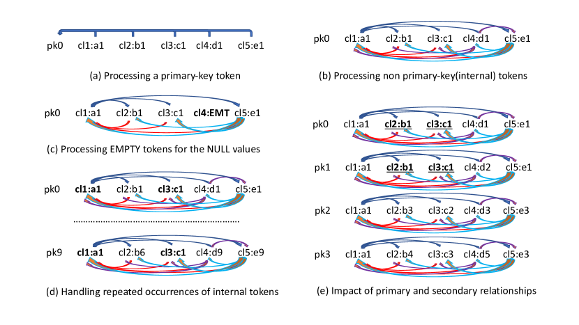
Figure 3. Capturing relationships in a database embedding model for primary (a), non-primary key (b), empty (c), repeated occurrences of tokens (d), and primary and secondary relationships between tokens (e)

These vectors are used by the semantic functions
(e.g., AI_SIMILARITY()) in the SQL Cognitive Intelligence (CI) queries (Figure 2) to extract semantic relationships between the relational values. The output of the semantic functions is a numeric semantic score which is then used to order the relational output (Figure 2). While the semantic score can provide some insights towards understanding the results of semantic functions, it is still an abstraction, and does not provide detailed reasoning on the causes for the semantic score. Therefore, it is necessary to understand the inner workings of the database embedding model.

db2Vec, like its counterparts in NLP such as word2Vec, generates embedding vectors where each vector encodes a distributed representation of inferred semantics of the corresponding text token (Mikolov et al., 2013). Every vector captures different attributes of the inferred semantics, created in part by contributions of other tokens within a context (neighborhood). The strength of a distributed relationship between tokens depends on how often these tokens co-occur within a context. Therefore, individual token occurrence and pair-wise co-occurrence counts become key markers for understanding influence of different tokens in the semantic model, and can be used to provide deeper insights into the results of semantic functions.

4. Interpretability Implementation and Usage

AI-DB collects the token occurrence statistics and applies them to provide detailed reasoning into the ranked results of the semantic SQL CI queries. Figure 1 illustrates the three stages of integrating the interpretability capability into the AI-DB execution pipeline. The first stage(1) operates on the textified training document by extracting the required token statistics and storing the information in a space-efficient manner (2). This information is then fetched at runtime for interpreting ranked results from a SQL CI query that invokes a semantic function (3). Given a ranked result list, the AI-DB interpretability component aims to identify (1) columns from the base relational view, and (2) values in the base table, that have the most influence on the results.

4.1. Token count Statistics

From the training process outlined in the previous Section, one can see that tokens with NULL values, as well as tokens associated with unique primary keys do not contribute to the training and vector generation of other tokens. Since the tokens are typed using the column names, it is possible to use the overall distribution of tokens across different columns to identify columns that play a significant role in the embedding process. To identify such columns, we have developed two aggregate metrics that use individual token counts to generate two per-column scores: Influence and Discriminatory scores.

4.1.1. Influence Score

The first metric, Influence Score, captures the collective influence of a particular column on the overall training as a measure of number of empty (EMT) tokens in that column. For a column $i$, it is calculated as a fraction of the number of EMT tokens to the total number of tokens in column $i$:

(1) $$Influence\_score(i)=1.0-\frac{Total(\#EMT\_Tokens(i))}{Total(\#Tokens(i))}$$

The numerical ratio, varies from $1.0$ (most influence, with no NULL values in a column) to $0$ (all NULL values in a column). The higher the influence score is for a column, the higher is the contribution of the values in that column to the trained model.

4.1.2. Discriminatory Score

The Discriminatory Score for a column $i$ captures the collective ability of that column (i.e., aggregated over all tokens in that column) to semantically distinguish another entity in the base relational view. If a token appears multiple times in a column (i.e., it occurs in multiple rows or contexts), its final inferred meaning is due to contributions from all of its neighboring tokens in the rows it where appears. Given a token, the larger the number of contributors is, lower is its ability to distinguish (or strongly relate) to any of the tokens. For example, in the unique primary key column, each token appears only once, and its inferred meaning is determined only by its neighbors in the associated row. On the other extreme, if a particular column contains only one token, its inferred meaning is determined by all other tokens in the training document. In such case, the ability of the token to be dominantly related to another token is greatly diminished. For a column $i$, the Discriminatory score is calculated as:

(2) $$Discriminatory\_score(i)=\frac{Total(\#Unique\_Tokens(i))}{Total(\#Tokens(i))}$$

The value of a column discriminatory score can vary from 1.0 (most discriminatory) to $\frac{1}{n}$ (least discriminatory), where $n$ is the total number of tokens in that column. One can also compute the discriminatory score per individual token, $tk_{i}$ as:

(3) $$Discriminatory\_score(tk_{i})=1.0-\frac{Total(\#Occurrences(tk_{i}))}{Total(\#Tokens(i))}$$

The per-token discriminatory score value varies from $(n-1)/n$ (most discriminatory) to $0$ (least discriminatory).

These two scores encapsulate key characteristics of a training document (i.e., overall importance of columns and unique tokens) and capture its impact on the trained model, and eventually on the quality of results from SQL CI queries. These scores can be used to improve any issues with the training document (e.g., neglect the column with a low influence score (lots of EMT tokens), or with low discriminatory score (fewer unique values in a column). The column and per-token discriminatory scores can also expose data skews in a column, and can be used to mitigate any negative impacts (e.g., bias). In addition to these scores, AI-DB provides detailed information about the numeric columns such as minimum and maximum values as well as cluster information such as cluster size, range, median, etc.

At runtime, for any semantic function used in the SQL CI query, these scores can identify the most(least) influential columns and tokens solely using the per-column token statistics for the model being used. Thus, the Influence and Discriminatory scores provide query-agnostic Model interpretability.

4.2. Token co-occurrence Statistics

The Influence and Discriminatory scores capture the overall importance of columns and unique tokens during training. Token co-occurrence counts, on the other hand, focus on capturing relationships between tokens associated with different types. As discussed in Section 3.1 and Figure 3, pair-wise relationships form the atomic building blocks for training the database embedding model. Thus, pair-wise (bi-gram) co-occurrence counts become a reliable tool for understanding the causes behind any db2Vec relationship at per-token granularity.

Table 1. Unique co-occurring token pairs

Datasets	Unique
	Token Pairs
Virginia	13,481,992
Fannie Mae	203,974
Airline	5,902
Mushroom	5,462
Credit Card Fraud	7,094,716
CA Toxicity	13,413,076

A typical database table may contain a fairly large number of entities, with potentially significant number of unique values. Assuming $n$ unique tokens in a training document, the number of possible pairs is $C(n,2)=\frac{n!}{(n-2)!2!}=\frac{n\times(n-1)}{2}\approx O(n^{2})$. In other words, the size of the co-occurrence matrix can be almost the square of the full vocabulary size! Table 1 illustrates the number of co-occurring tokens for a representative set of training datasets. For a larger value of $n$, this value is prohibitive and not all possible pairs can exist in a document. Therefore, solutions such as a naive array-based storage or a dictionary with full strings as keys, are both space inefficient and wasteful.

The solution is to employ a probabilistic counting data structure, called Sketch (Pitel and Fouquier, 2015; Cormode and Muthukrishnan, 2005a; Rinberg et al., 2019), to store and process the pair-wise co-occurrence counts. Data sketches are probabilistic structures originally designed to record aggregate counts of values in long-running (potentially infinite) streams (e.g., ad clicks) (Gibbons and Matias, 1999; Alon et al., 1996; Cormode and Muthukrishnan, 2005b). While sketches have been traditionally used for compression and compactly recording tokens in streams for prespecified queries, it is being applied to other domains such as NLP (Goyal et al., 2010) as well. Common uses typically supported are total counts of tokens seen in a stream or database, and a variety of algorithms, such the Count-Min (CM) sketch have been developed for this purpose. AI-DB uses the CM sketch for storing and processing the token co-occurrence counts.

Structurally, CM sketches are typically implemented as a two-dimensional table of with $h$ rows and $d$ columns. Each row corresponds to a different hash function over a range $d$. For every instance value to be recorded using $h$ independent hash functions, distinct positions are calculated for each of the $h$ rows, and their values incremented. At query time, for the token pair being queried, $h$ positions are first calculated, and then a count summarization is performed across the rows using the minimum function over the positions determined by the hash functions, returning an approximation of the total count. The minimum function helps to reduce the counting errors generated by the hash conflicts. In practice, sketches such as the CM sketch are shown to provide fairly accurate approximations of frequent item counts, but for low-frequency items the approximation errors can be significant (Thomas et al., 2009). A sketch with $h$ hash tables with range $d$ each, uses $O(h\times d)$ space, where $(h\times d)\ll n^{2}$. One could, conceivably, store the $O(n^{2})$ co-occurrence matrix using sparse matrix serialization techniques, but the sparse approach, in the worst case, would still require space for storing $\frac{n\times(n-1)}{2}$ non-null values.

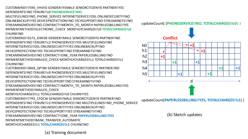
Figure 4. Co-occurrence sketch count updates: (a) extracting token-pairs from the source training document, (b) updating the sketch per token-pair. The red values denote positions of conflicts during sketch updates.

In our implementation, a CM-based co-occurrence sketch is populated with the token-pair co-occurrence values extracted from the textified document generated from a relational table (Figure 1(a)). For every ”sentence” in the training document (corresponds to a relational table row), each pair of tokens is selected (Figure 4). Then the CM co-occurrence sketch is updated as follows: (1) for the token-pair in consideration, $h$ positions are computed for each of the $h$ hash functions, and (2) each value in the corresponding position is incremented by 1 (Figure 1(b)). The increment value represents the strength of the relationships between the tokens in a token-pair. Since database embedding assumes that all tokens associated with a relational row are equally related to each other, irrespective of the token-pair, every sketch increment has the same value. Tokens corresponding to unique primary keys (e.g., CUSTOMERID), appear only once; hence any token pair containing such tokens is not stored in the co-occurrence sketch. It is possible that positions corresponding to different token pairs conflict (Figure 4). However, the query-time minimum function has been designed to return a value that reduces the approximation error by returning the minimum value from the positions corresponding to a token-pair. The implementation also uses a large hash function range, $d$. Larger the range is, the chances of conflict reduce, decreasing the approximation error, and the co-occurrence sketch becomes increasingly sparse.

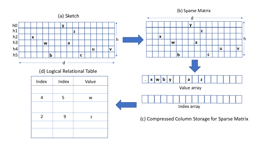
Figure 5. Co-occurrence sketch as a sparse matrix: (1) co-occurrence sketch, (2) sparse matrix representation, (3) CSR serialization, and (4) re-populating a logical relational table.

A benefit of using large sparse co-occurrence sketches is that they can be viewed as sparse matrices as shown in Figure 5. As such, one can use any of several existing sparse storage representations, e.g., Compressed Sparse Row (CSR) or Column (CSC) formats (Golub and Van Loan, 1996), for efficiently storing the co-occurrence sketch. The persistent size will be smaller than the in-memory representation and the space reduction will be determined by the co-occurrence sketch sparsity. Specifically, a sparse matrix serialization of a sketch with $h$ hash functions and range $d$, will store only $m$ non-null sketch values, where $m<(h\times d)\ll n^{2}$. The ability to increase the size while allowing the sparsity gives the best of both worlds: accuracy in interpretability, while allowing for space and performance afforded by sparse matrix techniques. Once the co-occurrence sketch is populated, it is serialized using the CSR sparse storage format that stores a matrix in a dense row-major order using two arrays. The sparse matrix formulation enables resurrection of the co-occurrence sketch as a logical relational table, where each row stores the row and column indices, along with the corresponding count value. At the time of interpreting results of a SQL CI query (Figure 1), this relational table can be queried to fetch the approximate counts of a token pair as follows: (1) For a token pair, compute the position index $j$ for each of the $h$ hash functions. (2) Use the hash (rows) index $i$, and the position index, $j$, to retrieve the approximate count value.

An advantage of co-occurrence sketches is that they are sufficiently accurate when the number of tokens is limited, and queries are made within those limited numbers of inserted tokens. If the universe of tokens used in queries (such as tokens never seen before by the co-occurrence sketch) is much larger than the co-occurrence sketch was designed for, the queries will produce inaccurate counts. This is common in database tables which have columns with a large number of possible entries (such as account numbers), and the total possible combinations, say in a database transaction tracking to and from accounts, each with $m$ and $n$ possible values would result in a large universe of $m\times n$ number of possible co-occurring tokens; although the actual number of co-occurrences in the database itself may be much smaller. Building sketches that store counts for the large universe of all possible token co-occurrences is prohibitive in terms of memory. To address this, we only query the count sketch for tokens that exist in the database, by using a Bloom filter-based (Mitzenmacher and Upfal, 2005) shadow boolean sketch described in the following Section.

The space efficiency of a sketch can further be improved, although with a small impact on accuracy, by thresholding small values in the sketch and setting them to zero. This makes the sketch sparser, enabling further reduction in the file size when the sketch is serialized using the CSR approach.

In addition to space efficiency, runtime performance is another major challenge facing the creation of sketches, especially as the associated table size grows. The sketch creation algorithm has to track the co-occurrence in every row, and therefore the runtime grows linearly with the size of the text file. Sketches are inherently distributive in nature. As long as the size of the sketch, and the hash functions for every row are the same, i.e., the sketches are compatible, they can be simply added together without loss of accuracy. Thus, speedup in processing can be achieved through parallelizing the sketch creation process. Each text file, can be split by rows into several non-overlapping chunks, and separate count sketches are generated for each chunk in parallel by separate threads. Once the sketch generation for the chunks is complete, the sketches generated by each thread are merged together by adding the entries in the sketches into a single top level sketch.

All the necessary steps required for initializing, populating, storing, and using the co-occurrence count sketch are built-in into the AI-DB processing flow (Figure 1) without using any external explainability tools or packages, and requires no user intervention.

4.3. Aggregate Statistics

While the sketch enables the computation of co-occurrences, another additional capability is the gathering of statistical information about important relationships between pairs of variables. In particular, for a given query token, the user may be interested in which other token has the highest co-occurrence with it, or interested in the median co-occurrences. While the sketch does not store actual strings of co-occurrence pairs themselves, all pairs of strings can be computed with the addition of a small datastructure that only maintains the valid values for each column. The additional data structure is a dictionary which has the column name as the key, and valid column categorical strings as the values. Using this data structure, for any given query token, other tokens that have maximum co-occurrences can be found.

Consider a query token for which the maximum value needs to be computed. From the dictionary, it is paired with all valid values for other columns. The pairs are checked in the shadow sketch for existence. If the shadow sketch decides that the pair exists, then the co-occurrence sketch is queried. This is done for all pairs that are generated from the dictionary for the given token, and the maximum is computed. A shadow sketch, maintained for aggregate statistics, is implemented as a Bloom Filter which returns a boolean value to indicate whether a token pair generated by combining any two tokens is actually present in the sketch (and was present in the training set in the first place). This shadow sketch is only needed when computing aggregate statistics.

4.4. Interpretability in Practice

Let’s describe how the AI-DB system uses the token count and co-occurrence statistics to interpret results of a SQL CI query. The AI-DB interpretability component (Figure 1) uses token occurrence statistics to provide query-agnostic column-oriented model interpretability and uses the pair-wise co-occurrence statistics to enable query-specific value-oriented function interpretability. The AI-DB function interpretability identifies specific values from the associated relational table that have the most impact on the behavior of an semantic similarity function invoked by a CI query.

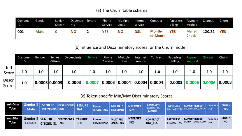
Figure 6. Influence and Discriminatory score for the Churn dataset. (a) Table schema with a sample row, (b) aggregated per-column influence and discriminatory scores, and (c) per-column min and max discriminatory scores.

This section describes the AI-DB interpretability capability using the publicly available Telecom Churn dataset (IBM, 2020). The Churn dataset describes customer characteristics of a hypothetical Telecom company. Figure 6(a) presents the Churn table schema: the table uses CustomerID as the primary key and contains information about the customer account, including if the customer is considered to be churned. For training the db2Vec model, the CustomerID column is defined as the key column, the Charges and Tenure columns are marked as the numerical columns, and the rest of the columns are marked as categorical. The values in the two numerical columns are clustered before training and replaced by tokens that represent clusters corresponding to the values. Figure 6(b) presents the per-column influence and discriminatory scores for the Churn table being trained. Since the table has no NULL values, all the columns have the highest influence score of 1.0. For the discriminator scores, the Tenure column has the largest number of unique values (i.e., the number of clusters), resulting in the second highest discriminatory score. The columns Payment Method, and Charges columns have the next highest discriminatory scores. The remaining columns have very low discriminatory score as the majority of columns only have binary values. Figure 6(c) presents per-column values with minimum and maximum discriminator scores: the values with maximum occurrences have the least discriminatory score, and vice versa. This information enables the user to determine if the data is skewed, and which value is over-represented. For example, from Figure 6(c), one can see that the dataset is skewed towards young and male customers, with relatively longer tenure (corresponding to the cluster c4), and paying high charges (corresponding to the cluster c2) that are more likely to churn. One can use the data skew information to update the raw dataset, or create a new view for training, or understand which columns and values impact the results.

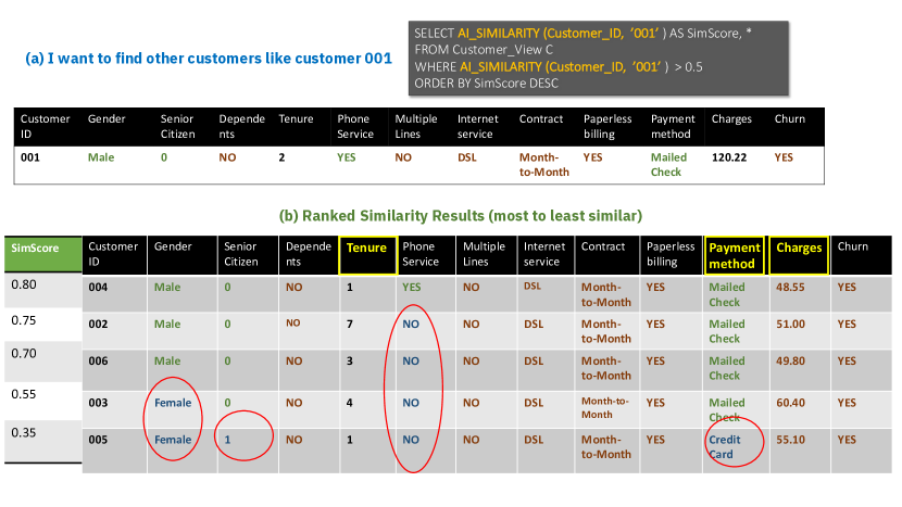
Figure 7. Invoking a primary key similarity query on the Churn dataset: (a) a sample semantic SQL query and the input row for customer 001, and (b) ranked result rows with the most influential highlighted columns.

AI-DB’s built-in interpretability feature is illustrated by two exemplar pair-wise similarity queries. The first type of query covers involves only primary key values and the second involves internal (no-primary) values (the other value can be either primary or internal value). The first example, Figure 7 (a), presents a SQL CI query to find customer IDs similar to an input customer ID (e.g., 001). The SQL CI query returns the output similarity score for the semantic function, AI_SIMILARITY as well as the values of other columns (Figure 7(b)). As the result shows, the most similar row has the highest similarity score (in this scenario, two primary key values are compared and the similarity score is the cosine similarity score between the corresponding vectors). Primary-key based co-occurrence values are not stored in the co-occurrence sketch, and as such only the model interpretability feature to understand results of the CI query. The row corresponding to the most similar customer ID, 004, matches in all categories with the row corresponding to customer 001. Numerical values corresponding to columns Tenure and Charges fall in the same range. Going down the ranked result list, it is observed that the rows have increasing differences. Furthermore, based on the influence and discriminatory scores, it is deduced that the Tenure, Payment Method, and Charges columns, have the most impact on the result ordering. We can also observe that using the per-token discriminator scores, the token, Tenure!!c0, corresponding to the very small tenure values, is the most impactful value in the result list.

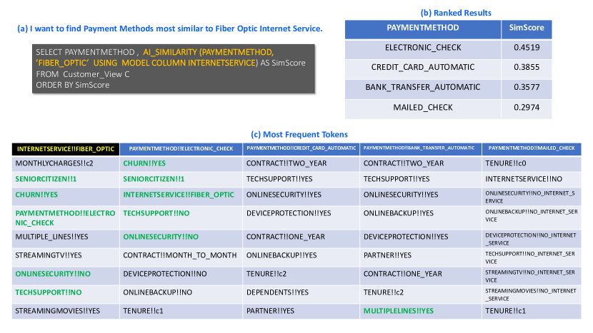
Figure 8. Invoking a similarity query on a non primary key value in the Churn dataset: (a) sample semantic SQL query, (b) sorted result, (c) most co-occurring tokens for the input and result values.

The second SQL CI query example, Figure 8(a), compares two non-primary key values, associated with two different columns: it aims to find the most related payment method to the FIBER_OPTIC internet service. Figure 8(b) presents the result list ordered by the similarity score. To get insights into which values and columns have the maximum impact on the sorted results, co-occurrence sketch is used. From this co-occurrence sketch, stored as an auxiliary relational table, more frequent tokens of associated with the key values in the query are obtained (Figure 8(c)). From this list, one can observe that ELECTRONIC_CHECK is the most frequent payment method associated with the FIBER_OPTIC internet service. Furthermore, ELECTRONIC_CHECK and FIBER_OPTIC share four frequently occurring neighbors. Thus, using the co-occurrence counts from the sketch, one can summarize that ELECTRONIC_CHECK is most related to FIBER_OPTIC due to the strong primary relationship between the tokens, and the secondary relationships generated by the common neighbors (Section 3.1).

In practice, these two approaches are generalized to enable interpretability for different semantic functions (e.g., dissimilarity, analogy, etc.) over either primary key or internal values. For example, for a dissimilarity query, the co-occurrence sketch can be used to identify the least co-occurring tokens to validate that output values reported from the query do not share any common neighbors. Thus, using the similarity scores, along with model and function interpretability capabilities, the AI-DB system is able provide in-database support to provide key insights into the results of the SQL CI queries.

AI-DB’s interpretability capability differs from the existing interpretability/explainability approaches (Section 2) in many ways. First, techniques outlined in this Section are designed for a self-supervised DL model that generates semantic embedded vectors to be used for answering a variety of similarity based queries. Although similar to vector embedding NLP models, the db2Vec model has key differences, e.g., support for non-text entities such as numeric values. Our approach provides both query-agnostic global model interpretability, as well as, query-specific local function interpretability. The db2Vec training approach provides hooks to extract key intrinsic information about interpretability (i.e., db2Vec has been designed and implemented as a self-describing model). We encode the relationships between the trained entities using intrinsic co-occurrence properties of the training data, and capture these relationships using a space-efficient sketch data structure. The per-token discriminator score, as well as the clustering information for the numeric columns, enables identification of specific input values that influence the results of semantic queries. Finally, the entire interpretability pipeline has been designed to be implemented within the context of a relational database such that the required information can be extracted from an input relational table, stored into an auxiliary relational table, and then used to interpret an SQL CI query using the auxiliary relational table (Figure 1). Our interpretability approach does not use any external tools and requires no user intervention.

5. Evaluation

The evaluation of the quality of the proposed co-occurrence sketch for functional interpretability as well as its runtime characteristics such as space consumption and sketch generation performance, is detailed in this Section. For this evaluation, a set of datasets is chosen, 10 pair-wise similarity queries for each dataset are run. The accuracy of the proposed sketch-based approach is evaluated for each query. An overview the selected datasets, description of the evaluation methodology, and experimental results are presented.

5.1. Evaluation Setup and Datasets

The performance of the probabilistic sketch is validated by comparing it’s result accuracy to a baseline approach that gives exact results obtained using complete co-occurrence information in memory. The baseline system ingests the complete training document as a Python Pandas dataframe, and computes co-occurrence statistics over the entire training set. The sketch approach on the other hand uses the Spark CountMinSketch Class (Apache Spark, 2022), while the update and reads from this data structure is performed with native Java. The code runs in Java native multithreading mode for the larger data sets. The experiments compare the baseline and sketch approaches and score the comparison using the NDCG metric. Both baseline and sketch approaches were implemented in the Python-based AI-DB system (Figure 1) and the experiments reported in this Section were run on x86/Linux machines.

For the experimental evaluation, 6 different datasets containing both real and synthetically generated data are used. An overview of some dataset basic statistics is provided in Table 2. In this table, the first two columns present the actual number of rows and columns in the source dataset. The third column presents the total number of non-primary key tokens and the last column reports the number of unique non-primary key tokens in the corresponding textified (Section 3) training dataset. Note that number of unique tokens depends on the input data characteristics: a dataset dominated by either categorical or numeric values tends to have fewer unique tokens after textification.

Table 2. Dataset structural characteristics: number of rows and columns along with counts of total and unique non-primary tokens

Dataset	Table Information		# Non-primary	# Non-primary
	Rows	Columns	Tokens	Unique Tokens
Virginia	1,371,968	8	12,347,712	1,452,156
Mushroom	61,069	21	1,343,518	139
Airline	129,880	23	3,117,120	115
Fannie Mae	11,232,359	20	235,879,539	1,475
Credit Card	14,820,425	15	237,126,800	111,752
CA Toxicity	1,248,836	88	111,146,404	92,567

The Virginia dataset (Commonwealth of Virginia, 2016) is a publicly available expenditure dataset from the State of Virginia for the 2015/2016 fiscal year. It lists details of every transaction such as vendor name, corresponding state agency, which government fund was used etc, by unique customers or vendors. Vendors can be individuals, and/or private and public institutions, such as county agencies, school districts, banks, businesses, etc.

Freddie Mac and Fannie Mae are two Government agencies that buy mortgages from lenders and hold them in portfolios or create sellable mortgage backed securities. The Fannie-Mae dataset (Fannie Mae, 2022) covers loan acquisition and performance data from 2007-2012 consisting of 30-year and less, fully amortizing, single-family, conventional fixed-rate mortgages.

The Credit Card transactional dataset (Altman, 2019) is a synthetically generated dataset that contains transactions of about 2000 customers with 40 fraudsters. Each row represents a unique transaction with 15 distinct attributes such as user id, card id, time based attributes, transaction amount, transaction type, transaction errors and finally merchant details like name, Merchant Category Code(MCC), city, state and zip code.

The CA Toxicity dataset (State of California, 2021) reports results of toxicity measurements for surface water performed at different locations in the State of California. The Airline Passenger Satisfaction dataset (Klein, 2020) contains airline passenger satisfaction survey covering different aspects of airline travel experience (e.g., service, delays, distance, travel class, on-board features, etc.) The UCI Mushroom dataset (UCI Data Team, 2019) contains information on 23 species of mushrooms such as physical, visual and olfactory features of each specimen as well as habitat and growth pattern information and whether the specimen is edible or not.

5.2. Evaluation Methodology

For each dataset, ten different pair-wise similarity queries were performed. These queries covered inter- and intra-column query patterns over non-primary keys (Section 4.4). Given an input dataset, it is first converted to a text training document used as the input to generate probabilistic co-occurrence sketch as well as a precise, but space consuming, co-occurrence data structure. Using these two data structures, the top co-occurring tokens are computed for the input query parameter and the result values from the corresponding training text file. Co-occurrences for each of the query and results are limited to the top five columns of interest in the corresponding relational table and are presented in sorted order. The exact results serve as a baseline for comparison and validation of the approximate results from the probabilistic co-occurrence sketch.

The exact and approximate lists are then compared using the Normalized Discounted Cumulative Gain (NDCG) (Järvelin and Kekäläinen, 2002) metric. NDCG is a widely used metric to evaluate search results in order of relevance. NDCG compares not only a sequence of results, but the sorted order of relevance in which they are presented as well. The NDCG score used in this paper differs from the traditional computation in two important ways. First, there are no repeated values, and second, an additional penalty parameter is added that reduces the NDCG score in proportion to the difference in expected and observed positions. The higher the NDCG score is, the higher is the matching, both in the values in the list, and its order. An NDCG score of 1.0 means that both lists contain the same entries in the same order.

To illustrate this evaluation approach, an example for the Virginia dataset is used: Figure 9(a) shows an intra-column query comparing a specified vendor, A_COMPUTER with other vendors. Figure 9(b) shows the corresponding JSON representation. The keyword q1 denotes the intra-column similarity query, ip denotes the token on which the similarity query was performed, op denotes the tokens obtained as results from AI-DB for the query, and columns shows the table columns of interest for the input parameter. For the query q1, five columns were specified as of interest to the user.

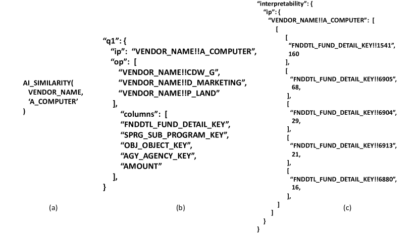
Figure 9. Example of one of the queries for the Virginia dataset (a), JSON representation of the results (b), and co-occurrence results (c)

Figure 9(c) gives a small exemplary snippet (due to paper space limitations) of the interpretability co-occurrence results for the query in Figure 9(a). The snippet shows the co-occurrence results (tokens and their co-occurrence counts) for one column,
FNDDTL_FUND_DETAIL_KEY, in sorted order for the input parameter VENDOR_NAME!!A_COMPUTER. As discussed in Figure 8, functional interpretability requires the list of most co-occurring tokens both for the input and result values (e.g., VENDOR_NAME!!CDW_G). Therefore, the full JSON file stores similar key-value results for each input and result values of each similarity query (Figure 9(a)), for each of the top five selected columns. Once the JSON files are generated, JSON files for the same set of query inputs as well as output results are scored for the baseline and the sketch scenarios. The scoring is based on NDCG comparison of the sorted lists for each input query, and result as described earlier, and an average of the scores for that experiment are presented.

5.3. Evaluation Results

In this section, the behavior of the co-occurrence sketch along three dimensions is evaluated: relative accuracy for the queries as defined by the NDCG metric, space utilization, and multithreaded scalability.

Evaluating Space Utilization:

Table 2 gives insight into the structural aspects of the textified training files that are used to generate the co-occurrence sketch. Parameters of interest such as number of database table rows, number of total tokens, and number of unique tokens (vocabulary) are presented. These parameters provide an insight into the challenges in creating a co-occurrence sketch for the dataset. While the number of lines in the textified file decides the total time for data parsing and creating the co-occurrence sketch, the number of unique tokens and the related number of co-occurrences of tokens impacts the size of co-occurrence sketch (as well as the likelihood of hash conflicts in a less than sufficient sized sketch).

Table 3. Space savings with co-occurrence sketch (using 5 hash functions with NDCG of 0.95 or higher). Sketch range $d$ in millions (M). Sparse file stored in the CSR format.

Dataset	Estimated Space(MB)	Sparse File Size(MB)	Co-occurrence Sketch	Space
	for Token Pairs	for Co-occurrence Sketch	Range (M) $d$	Saving
Virginia	448	58.2	8	7.82
Mushroom	0.46	0.074	0.1	6.21
Airline	0.33	0.052	0.1	6.34
Fannie Mae	17.94	2.8	4	6.4
Credit Card	424.84	64.78	16	6.57
CA Toxicity	640.72	71.8	32	8.92

Table 3 illustrates the space savings provided by the sketch as compared to the estimated space for storing the co-occurrence values as a dictionary in Java. There are several potential ways to track co-occurrences. First, a textified file (which is an entire database table in text form) may be stored in memory and co-occurrences calculated on demand, but this is inefficient and prohibitive from a memory standpoint. Another possibility is a dictionary based data structure, where each co-occurring pair of tokens in the data set is maintained a key with the total count for that co-occurring token as the value. In any data set, the number of pairs of tokens can be quite large, making a dictionary approach also inefficient for storage in memory, although it would be definitely preferable to storing the entire database table.

The sketch on the other hand, does not store the actual string for the co-occurring pair. Instead, it uses a hash on the string to identify locations in the arrays to maintain the counts. In hash based data structures, there is a trade-off between accuracy due to has hash conflicts and size of the structure. The results in Table 3 compare the size of a sketch that provides an NDCG accuracy of at least 0.95 when compared to an estimate of the conservative base case of storing the data structure as a dictionary.

As can be seen from the results, a gain of 5x-10x in memory area was achieved with the sketch as compared to a dictionary data structure for an NDCG accuracy score of 0.95 or greater. The memory savings are significantly even higher for lower but acceptable NDCG accuracy scores. Since the use of the sketch is for interpretability of results already produced by the semantic functions, small variations in sorted order have lower impact on the interpretability quality.

Evaluating Sketch Accuracy:

As with any approach based on hashing, increasing the size of the data structure reduces hash conflicts, and therefore improves accuracy. Count-min structures with multiple rows improve the accuracy of hashing for smaller sized data structures while allowing some amount of hashing conflict within a given location. By using a Count-min sketch, we keep the accuracy higher even with smaller sizes for the rows, and allowing for some hash conflict. Table 4 gives the accuracy sensitivity of a sketch for the Virginia, Fannie Mae and CA Toxicity datasets.

Table 4. Accuracy vs. space utilization for Virginia, Fannie Mae, and CA Toxicity datasets. The co-occurrence sketch is using 5 hash functions ($h=5$). Sketch range $d$ in millions (M).

Virginia		Fannie Mae		CA Toxicity
Sketch Range (M)	NDCG	Sketch Range (M)	NDCG	Sketch Range (M)	NDCG
$d$	Accuracy	$d$	Accuracy	$d$	Accuracy
1	0.56	0.03	0.58	0.125	0.54
2	0.56	0.06	0.66	0.5	0.56
3	0.62	0.125	0.69	1	0.67
4	0.64	0.25	0.76	2	0.76
5	0.79	0.5	0.83	4	0.83
6	0.78	1	0.86	6	0.90
7	0.81	2	0.92	8	0.92
8	0.99	3	0.94	16	0.93
9	0.99	4	0.95	24	0.94
10	0.99	5	0.99	32	0.97

As described earlier with regard to accuracy with space trade-off, the size of the in-memory co-occurrence sketch can be grown to increase accuracy, and due to the sparsity of the structure, the overall file space required can still be managed. Table 5 gives the percentage of the sketch that stores the zero value for NDCG accuracy targets of 0.95 and 0.99. In Table 5, the Sketch Range column reflects an effort to increase the accuracy of the probabilistic co-occurrence sketch to 0.95 and above by increasing the number of entries in the hash range $d$ (values reported in units of millions (M)). The CSR sparse matrix file size is compared against the total area of the in-memory sketch for each of these target accuracies. Due to the sparsity of the sketch data structure, it is possible to compress the space using a sparse matrix representation while targeting high accuracy from the sketch. With the increased accuracy targets of 0.99, significantly larger sketches are required (in a few datasets double), but overall the CSR size increases by a much smaller amount. The increased sparsity helps to improve accuracy by managing the overhead of storing these sketch tables in a relational database table during runtime.

Table 5. Sparsity with sketch sizes for NDCG values: 0.95 and 0.99. Sketch range $d$ in millions (M). Sparse file stored in the CSR format.

Dataset	NDCG=0.95				NDCG=0.99
	Sketch	Full Sketch	Sparse File	Sparsity	Sketch	Full Sketch	Sparse File	Sparsity
	Range(M) $d$	Size (MB)	Size (MB)	% Zero Values	Range(M) $d$	Size (MB)	Size (MB)	% Zero Values
Virginia	8	160	58.2	63	16	320	78.4	75
Mushroom	0.1	1	0.074	92	0.1	2	0.18	91
Airline	0.1	1	0.052	94	0.1	2	0.14	93
Fannie Mae	4	80	2.8	96	5	100	3.1	97
Credit Card	16	320	64.78	79	32	640	77.0	88
CA Toxicity	32	640	71.8	89	64	1280	104	92

Evaluating Runtime Scalability:

The sketch data structure is inherently distributive. Sketches can be created from mutually exclusive subgroups of database rows or lines of a textified file of a dataset. The individual sketches generated from different groups of lines can be then merged without locking, simply by adding together the values at each array position into a single sketch, as long as each individual table has the same dimension and each row has the same hash function across the different sketches. If each of the individual sketches is a two-dimensional vector of the same dimension and each row is also associated with the same hash function across the table vectors, the resulting sketch is a vector addition of the individual vectors.

Table 6 provides the amount of time taken to build the sketch. For the relatively smaller data sets, e.g., Virginia, single threaded runs were used. For larger datasets such as Fannie Mae, Credit Card, and CA Toxicity, Table 6 reports the sketch-building runtimes. The number of threads represents the thread count, after which multiprocessing scaling improvements become insignificant. Figure 10 gives the improvements for the Credit Card data set (one the larger data sets) with multithreading. In this particular test case, the scaling improvements tend to level off after about 5 threads, due to the overhead in creating a full sized sketch with each thread, and the costs of merging as each thread requires it’s own copy of a full sized sketch. Experimental data demonstrated that the co-occurrence data structure provides accurate results with space-efficient footprint and scalable build performance.

Table 6. Sketch build runtime (in milliseconds) along with the corresponding number of threads

Dataset	Build Time	# Threads
	milliseconds
Virginia	94,137	1
Mushroom	21,688	1
Airline	29,063	1
Fannie Mae	5,587,096	5
Credit Card	2,952,080	6
CA Toxicity	7,419,687	5

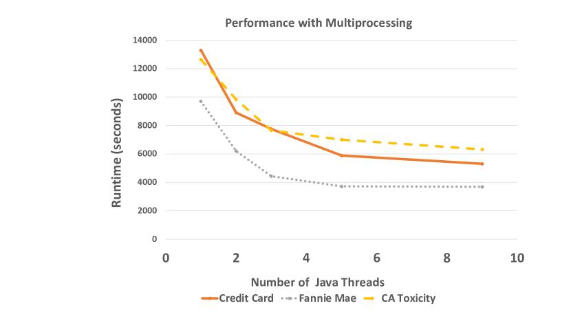
Figure 10. Scaling the co-occurrence sketch generation using multiple Java threads. Performance scaling reduces for the number of threads greater than 5.

6. Conclusions

A novel in-database interpretability system for providing detailed insights on the results of semantic SQL (CI) queries is presented. This capability has been designed to support a self-supervised vector embedding model that can be trained over very large database tables. A novel design that uses a probabilistic Count-Min sketch data structure to store the data co-occurrence information using a sparse-matrix data serialization format (CSR) is introduced. The sketch is materialized at runtime as a relational table which is queried for analyzing results of semantic functions. Experimental evaluation on a set of large and distinct datasets demonstrated that the sketch data structure provides a space-efficient and scalable approach to provide accurate interpretability results. As a future work, techniques for reducing Sketch conflicts using the Frequency-aware Count-Min (FCM) approach (Thomas et al., 2009), as well as enhancing the core interpretability capabilities to support new semantic queries will be investigated.

7. Acknowledgments

The authors thank Jose Neves, Matt Tong, and Wei Zhang for their detailed comments on the earlier versions of this paper.

References

- (1)
- Allen and Hospedales (2019) Carl Allen and Timothy M. Hospedales. 2019. Analogies Explained: Towards Understanding Word Embeddings. CoRR abs/1901.09813 (2019). arXiv:1901.09813 http://arxiv.org/abs/1901.09813
- Alon et al. (1996) Noga Alon, Yossi Matias, and Mario Szegedy. 1996. The Space Complexity of Approximating the Frequency Moments. In ACM Symposium on Theory of Computing. 20–29.
- Altman (2019) Erik Altman. 2019. Credit Card Transactions Dataset. https://www.kaggle.com/datasets/ealtman2019/credit-card-transactions
- Apache Spark (2022) Apache Spark. 2022. Online documentation. https://spark.apache.org/docs/preview/api/java/org/apache/spark/util/sketch/CountMinSketch.html
- Arrieta et al. (2019) Alejandro Barredo Arrieta, Natalia Díaz Rodríguez, Javier Del Ser, Adrien Bennetot, Siham Tabik, Alberto Barbado, Salvador García, Sergio Gil-Lopez, Daniel Molina, Richard Benjamins, Raja Chatila, and Francisco Herrera. 2019. Explainable Artificial Intelligence (XAI): Concepts, Taxonomies, Opportunities and Challenges toward Responsible AI. CoRR abs/1910.10045 (2019). arXiv:1910.10045 http://arxiv.org/abs/1910.10045
- Bahdanau et al. (2014) Dzmitry Bahdanau, Kyunghyun Cho, and Yoshua Bengio. 2014. Neural Machine Translation by Jointly Learning to Align and Translate. https://doi.org/10.48550/ARXIV.1409.0473
- Belinkov and Glass (2018) Yonatan Belinkov and James R. Glass. 2018. Analysis Methods in Neural Language Processing: A Survey. CoRR abs/1812.08951 (2018). arXiv:1812.08951 http://arxiv.org/abs/1812.08951
- Bibal et al. (2022) Adrien Bibal, Rémi Cardon, David Alfter, Rodrigo Wilkens, Xiaoou Wang, Thomas François, and Patrick Watrin. 2022. Is Attention Explanation? An Introduction to the Debate. In Proceedings of the 60th Annual Meeting of the Association for Computational Linguistics (Volume 1: Long Papers). Association for Computational Linguistics, Dublin, Ireland, 3889–3900. https://doi.org/10.18653/v1/2022.acl-long.269
- Bordawekar (2018) Rajesh Bordawekar. 2018. Cognitive Database: An Apache Spark-Based AI-Enabled Relational Database System. Spark Data+AI Summit.
- Bordawekar and Shmueli (2016) Rajesh Bordawekar and Oded Shmueli. 2016. Enabling Cognitive Intelligence Queries in Relational Databases using Low-dimensional Word Embeddings. CoRR abs/1603.07185 (2016). http://arxiv.org/abs/1603.07185
- Bordawekar and Shmueli (2017) Rajesh Bordawekar and Oded Shmueli. 2017. Using Word Embedding to Enable Semantic Queries in Relational Databases. In Proceedings of the 1st Workshop on Data Management for End-to-End Machine Learning (Chicago, IL, USA) (DEEM’17). ACM, New York, NY, USA, Article 5, 4 pages. https://doi.org/10.1145/3076246.3076251
- Celli (2021) Fabio Celli. 2021. Lex2vec: making Explainable Word Embedding via Distant Supervision. CoRR abs/2103.02269 (2021). arXiv:2103.02269 https://arxiv.org/abs/2103.02269
- Church and Hanks (1990) Kenneth Ward Church and Patrick Hanks. 1990. Word Association Norms, Mutual Information, and Lexicography. Computational Linguistics 16, 1 (1990), 22–29. https://aclanthology.org/J90-1003
- Commonwealth of Virginia (2016) Commonwealth of Virginia. 2016. State of virginia 2016 expenditures. https://www.datapoint.apa.virginia.gov
- Cormode and Muthukrishnan (2005a) Graham Cormode and S. Muthukrishnan. 2005a. An improved data stream summary: the count-min sketch and its applications. J. Algorithms 55, 1 (2005), 58–75. http://dblp.uni-trier.de/db/journals/jal/jal55.html#CormodeM05
- Cormode and Muthukrishnan (2005b) Graham Cormode and S. Muthukrishnan. 2005b. What’s Hot and What’s Not: Tracking Most Frequent Items Dynamically. ACM Transactions on Database Systems 30, 1 (March 2005), 249–278.
- Danilevsky et al. (2020) Marina Danilevsky, Kun Qian, Ranit Aharonov, Yannis Katsis, Ban Kawas, and Prithviraj Sen. 2020. A Survey of the State of Explainable AI for Natural Language Processing. CoRR abs/2010.00711 (2020). arXiv:2010.00711 https://arxiv.org/abs/2010.00711
- Date (1982) C. J. Date. 1982. A Formal Definition of the relational Model. SIGMOD Rec. 13, 1 (1982), 18–29. https://doi.org/10.1145/984514.984515
- Du et al. (2020) Mengnan Du, Ninghao Liu, and Xia Hu. 2020. Techniques for interpretable machine learning. Commun. ACM 63, 1 (January 2020).
- Face (2023) Hugging Face. 2023. Hugging Face Models. https://huggingface.co/models
- Fannie Mae (2022) Fannie Mae. 2022. Fannie Mae Single-Family Loan Performance Data. https://capitalmarkets.fanniemae.com/credit-risk-transfer/single-family-credit-risk-transfer/fannie-mae-single-family-loan-performance-data
- Gibbons and Matias (1999) Phillip B. Gibbons and Yossi Matias. 1999. Synopsis Data Structures for Massive Data Sets. In Proceedings of Symposium on Discrete Algorithms.
- Gilpin et al. (2018) Leilani H. Gilpin, David Bau, Ben Z. Yuan, Ayesha Bajwa, Michael A. Specter, and Lalana Kagal. 2018. Explaining Explanations: An Approach to Evaluating Interpretability of Machine Learning. CoRR abs/1806.00069 (2018). arXiv:1806.00069 http://arxiv.org/abs/1806.00069
- Golub and Van Loan (1996) Gene Golub and Charles Van Loan. 1996. Matrix Computations (3rd ed.). Johns Hopkins, Baltimore, Maryland.
- Goyal et al. (2010) Amit Goyal, Jagadeesh Jagarlamudi, Hal Daumé III, and Suresh Venkatasubramanian. 2010. Sketching Techniques for Large Scale NLP. In Proceedings of the NAACL HLT 2010 Sixth Web as Corpus Workshop. Association for Computational Linguistics, NAACL-HLT, Los Angeles, 17–25. https://aclanthology.org/W10-1503
- Ho (2022) Tin Kam Ho. 2022. Complexity of Representations in Deep Learning. (2022). https://doi.org/10.48550/ARXIV.2209.00525
- IBM (2020) IBM. 2020. Predict Customer Churn using Watson Machine Learning and Jupyter Notebooks on Cloud Pak for Data. https://github.com/IBM/telco-customer-churn-on-icp4d Apache-2.0 License.
- IBM (2022) IBM. 2022. IBM Z Artificial Intelligence Data Embedding Library. IBM z/OS 2.5.0 Online Documentation.
- IBM Db2 13 Project Team (2022) IBM Db2 13 Project Team. 2022. IBM Db2 13 for z/OS and More. IBM Redbook. https://www.ibm.com/products/db2-for-zos
- Jain and Wallace (2019) Sarthak Jain and Byron C. Wallace. 2019. Attention is not Explanation. CoRR abs/1902.10186 (2019). arXiv:1902.10186 http://arxiv.org/abs/1902.10186
- Järvelin and Kekäläinen (2002) Kalervo Järvelin and Jaana Kekäläinen. 2002. Cumulated Gain-Based Evaluation of IR Techniques. ACM Trans. Inf. Syst. 20, 4 (oct 2002), 422–446. https://doi.org/10.1145/582415.582418
- Karl Pearson (1901) Karl Pearson. 1901. LIII. On lines and planes of closest fit to systems of points in space. The London, Edinburgh, and Dublin Philosophical Magazine and Journal of Science 2, 11 (1901), 559–572. https://doi.org/10.1080/14786440109462720 arXiv:https://doi.org/10.1080/14786440109462720
- Klein (2020) T. J. Klein. 2020. Airline Passenger Satisfaction dataset. https://www.kaggle.com/datasets/teejmahal20/airline-passenger-satisfaction
- Lundberg and Lee (2017) Scott M. Lundberg and Su-In Lee. 2017. A unified approach to interpreting model predictions. CoRR abs/1705.07874 (2017). arXiv:1705.07874 http://arxiv.org/abs/1705.07874
- Madsen et al. (2021) Andreas Madsen, Siva Reddy, and Sarath Chandar. 2021. Post-hoc Interpretability for Neural NLP: A Survey. CoRR abs/2108.04840 (2021). arXiv:2108.04840 https://arxiv.org/abs/2108.04840
- Marcinkevics and Vogt (2020) Ricards Marcinkevics and Julia E. Vogt. 2020. Interpretability and Explainability: A Machine Learning Zoo Mini-tour. CoRR abs/2012.01805 (2020). arXiv:2012.01805 https://arxiv.org/abs/2012.01805
- Mikolov et al. (2013) Tomas Mikolov, Ilya Sutskever, Kai Chen, Gregory S. Corrado, and Jeffrey Dean. 2013. Distributed Representations of Words and Phrases and their Compositionality. In 27th Annual Conference on Neural Information Processing Systems 2013. 3111–3119.
- Mitzenmacher and Upfal (2005) Michael Mitzenmacher and Eli Upfal. 2005. Probability and Computing: Randomized Algorithms and Probabilistic Analysis. Cambridge University Press.
- Molnar (2022) Christoph Molnar. 2022. Interpretable Machine Learning. https://christophm.github.io/interpretable-ml-book
- Neelakantan et al. (2022) Arvind Neelakantan, Tao Xu, Raul Puri, Alec Radford, Jesse Michael Han, Jerry Tworek, Qiming Yuan, Nikolas Tezak, Jong Wook Kim, Chris Hallacy, Johannes Heidecke, Pranav Shyam, Boris Power, Tyna Eloundou Nekoul, Girish Sastry, Gretchen Krueger, David Schnurr, Felipe Petroski Such, Kenny Hsu, Madeleine Thompson, Tabarak Khan, Toki Sherbakov, Joanne Jang, Peter Welinder, and Lilian Weng. 2022. Text and Code Embeddings by Contrastive Pre-Training. CoRR abs/2201.10005 (2022). arXiv:2201.10005 https://arxiv.org/abs/2201.10005
- Neves et al. (2019) Jose Neves, Rajesh Bordawekar, and Elpida Tzortzatos. 2019. Demonstrating Semantic SQL Queries over Relational Data using the AI-Powered Database. In Proceedings of the 1st International Workshop on Applied AI for Database Systems and Applications (AIDB’19).
- Nvidia (2023) Nvidia. 2023. Explore NVIDIA NeMo LLM Service. https://www.nvidia.com/en-us/deep-learning-ai/solutions/large-language-models
- Park et al. (2017) Sungjoon Park, JinYeong Bak, and Alice Oh. 2017. Rotated Word Vector Representations and their Interpretability. In Proceedings of the 2017 Conference on Empirical Methods in Natural Language Processing. Association for Computational Linguistics, Copenhagen, Denmark, 401–411. https://doi.org/10.18653/v1/D17-1041
- Pennington et al. (2014) Jeffrey Pennington, Richard Socher, and Christopher D. Manning. 2014. GloVe: Global Vectors for Word Representation. In Proceedings of the 2014 Conference on Empirical Methods in Natural Language Processing. 1532–1543. http://aclweb.org/anthology/D/D14/D14-1162.pdf
- Pitel and Fouquier (2015) Guillaume Pitel and Geoffroy Fouquier. 2015. Count-Min-Log sketch: Approximately counting with approximate counters. CoRR abs/1502.04885 (2015). arXiv:1502.04885 http://arxiv.org/abs/1502.04885
- Ribeiro et al. (2016) Marco Tulio Ribeiro, Sameer Singh, and Carlos Guestrin. 2016. ”Why should I trust you?” Explaining the predictions of any classifier. In Proceedings of the 22nd ACM SIGKDD international conference on knowledge discovery and data mining. 1135–1144.
- Rinberg et al. (2019) Arik Rinberg, Alexander Spiegelman, Edward Bortnikov, Eshcar Hillel, Idit Keidar, and Hadar Serviansky. 2019. Fast Concurrent Data Sketches. CoRR abs/1902.10995 (2019). arXiv:1902.10995 http://arxiv.org/abs/1902.10995
- Rogers et al. (2020) Anna Rogers, Olga Kovaleva, and Anna Rumshisky. 2020. A Primer in BERTology: What we know about how BERT works. CoRR abs/2002.12327 (2020). arXiv:2002.12327 https://arxiv.org/abs/2002.12327
- Rudin (2019) Cynthia Rudin. 2019. Stop explaining black box machine learning models for high stakes decisions and use interpretable models instead. Nature Machine Intelligence (May 2019), 206–215.
- State of California (2021) State of California. 2021. Surface Water - Toxicity Results. https://data.cnra.ca.gov/dataset/surface-water-toxicity-results
- Subramanian et al. (2017) Anant Subramanian, Danish Pruthi, Harsh Jhamtani, Taylor Berg-Kirkpatrick, and Eduard H. Hovy. 2017. SPINE: SParse Interpretable Neural Embeddings. CoRR abs/1711.08792 (2017). arXiv:1711.08792 http://arxiv.org/abs/1711.08792
- Thomas et al. (2009) Dina Thomas, Rajesh Bordawekar, Charu C. Aggarwal, and Philip S. Yu. 2009. On Efficient Query Processing of Stream Counts on the Cell Processor. In 2009 IEEE 25th International Conference on Data Engineering. 748–759. https://doi.org/10.1109/ICDE.2009.35
- UCI Data Team (2019) UCI Data Team. 2019. UCI Mashroom Data. https://www.kaggle.com/code/aavigan/uci-mushroom-data
- van der Maaten and Hinton (2008) Laurens van der Maaten and Geoffrey Hinton. 2008. Visualizing Data using t-SNE. Journal of Machine Learning Research 9, 86 (2008), 2579–2605. http://jmlr.org/papers/v9/vandermaaten08a.html
- Vaswani et al. (2017) Ashish Vaswani, Noam Shazeer, Niki Parmar, Jakob Uszkoreit, Llion Jones, Aidan N. Gomez, Lukasz Kaiser, and Illia Polosukhin. 2017. Attention Is All You Need. arXiv:1706.03762 [cs.CL]
- Wiegreffe and Pinter (2019) Sarah Wiegreffe and Yuval Pinter. 2019. Attention is not not Explanation. CoRR abs/1908.04626 (2019). arXiv:1908.04626 http://arxiv.org/abs/1908.04626
- Zhang et al. (2019) Haitong Zhang, Yongping Du, Jiaxin Sun, and Qingxiao Li. 2019. Improving Interpretability of Word Embeddings by Generating Definition and Usage. CoRR abs/1912.05898 (2019). arXiv:1912.05898 http://arxiv.org/abs/1912.05898
- Zhang et al. (2020) Yu Zhang, Peter Tiño, Ales Leonardis, and Ke Tang. 2020. A Survey on Neural Network Interpretability. CoRR abs/2012.14261 (2020). arXiv:2012.14261 https://arxiv.org/abs/2012.14261