EquiPocket: an E(3)-Equivariant Geometric Graph Neural Network for Ligand Binding Site Prediction

Abstract.

Predicting the binding sites of the target proteins plays a fundamental role in drug discovery. Most existing deep-learning methods consider a protein as a 3D image by spatially clustering its atoms into voxels and then feed the voxelized protein into a 3D CNN for prediction. However, the CNN-based methods encounter several critical issues: 1) defective in representing irregular protein structures; 2) sensitive to rotations; 3) insufficient to characterize the protein surface; 4) unaware of data distribution shift. To address the above issues, this work proposes EquiPocket, an E(3)-equivariant Graph Neural Network (GNN) for binding site prediction. In particular, EquiPocket consists of three modules: the first one to extract local geometric information for each surface atom, the second one to model both the chemical and spatial structure of the protein, and the last one to capture the geometry of the surface via equivariant message passing over the surface atoms. We further propose a dense attention output layer to better alleviate the data distribution shift effect incurred by the variable protein size. Extensive experiments on several representative benchmarks demonstrate the superiority of our framework to the state-of-the-art methods.

1. Introduction

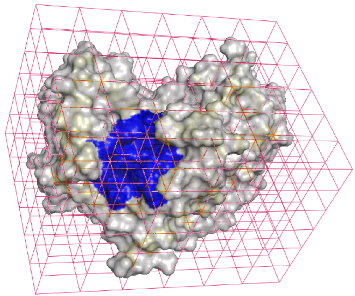
(a) Previous CNN-based methods by voxelization

(b) Our EquiPocket directly on protein graph

Figure 1. Illustrative comparison between previous CNN-based methods and our EquiPocket.

Nearly all biological and pharmacological processes in living systems involve interactions between receptors (i.e. target proteins) and ligands (i.e. small molecules or other proteins) (Rang, 2006). The places where such interactions occur are known as the binding sites/pockets of the ligands on the target protein structures, which are essential to determine whether or not the ligands are druggable and functionally relevant. Moreover, the knowledge of the binding site is able to facilitate many downstream tasks, such as docking (Zhang et al., 2022), the design of drug molecules (Wang et al., 2000), etc. Therefore, predicting the binding sites of the target proteins via in-silico algorithms forms an indispensable and even the first step in drug discovery.

Through the past years, plenty of computational methods have been proposed to detect binding sites, which can be roughly classified into three categories (Macari et al., 2019): the geometry-based (Levitt and Banaszak, 1992; Hendlich et al., 1997; Weisel et al., 2007; Le Guilloux et al., 2009; Chen et al., 2011; Dias et al., 2017), the probe-energy-based (Laskowski, 1995; Laurie and Jackson, 2005; Ngan et al., 2012; Faller et al., 2015) and the template-based (Brylinski and Skolnick, 2008; Toti et al., 2018). The computational methods exploit hand-crafted algorithmic procedures guided by domain knowledge or external templates, leading to insufficient expressivity in representing complicated proteins. Recently, with the accumulation of labeled data and the development of machine learning techniques, the learning-based approaches have been developed (Krivák and Hoksza, 2018), which manage to analyze and extract the underlying patterns of the input data that eventually align with the assign labels through the iterative process of learning. Although the learning-based methods have exhibited clear superiority over the classical computational counterparts, their performance and flexibility are still limited by the hand-crafted input features and the insufficiently-expressive models they used (Krivák and Hoksza, 2018).

More recently, motivated by the breakthrough of deep learning in a variety of fields, Convolutional Neural Networks (CNNs) have been applied successfully for the prediction of binding sites (Kandel et al., 2021). Typical works include DeepSite (Jiménez et al., 2017), DeepPocket (Aggarwal et al., 2021), DeepSurf (Mylonas et al., 2021), etc. The CNN-based methods consider a protein as a 3D image by spatially clustering its atoms into the nearest voxels, and then model the binding site prediction as a object detection problem or a semantic segmentation task on 3D grids. Thanks to the multi-layer and end-to-end learning paradigm, the CNN-based methods are observed to outperform traditional learning-based approaches and generally achieve the best performance on several public benchmarks (Mylonas et al., 2021).

In spite of the impressive progress, existing CNN-based models still encounter several issues as below:
Issue 1. Defective in leveraging regular voxels to model the proteins of irregular shape. First, a considerable number of voxels probably contain no atom since the protein atoms are unevenly distributed in space, which yields unnecessary redundancy in computation and memory. Moreover, the voxelization is usually constrained within a fixed-size space (e.g. $70\textup{\AA}\times 70\textup{\AA}\times 70\textup{\AA}$ ) (Jiménez et al., 2017; Stepniewska-Dziubinska et al., 2020). The atoms beyond this size will be directly discarded, resulting in incomplete and inaccurate modeling particularly for large proteins. Besides, although the voxelization process is able to encode certain spatial structure of the protein, it overlooks the irregular chemical interactions (i.e. the chemical bonds) between atoms and the topological structure upon that is also useful for binding site detection.
Issue 2. Sensitive to rotations. To discretize the protein into 3D grids, the CNN methods fix the three bases of the coordinates beforehand. When rotating the protein, the voxelization results could be distinct, and the predicted binding sites will change, which, however, conflicts with the fact that any rotation of the protein keeps the binding sites invariant. While it can be alleviated by the local grid (Mylonas et al., 2021) or augmenting training data with random rotations (Ragoza et al., 2017; Stepniewska-Dziubinska et al., 2020), which yet is data-dependent and unable to guarantee rotation invariance in theory.
Issue 3. Insufficient to characterize the geometry of the protein surface. The surface atoms comprise the major part of the binding pocket, which should be elaborately modeled. In the CNN-based methods, the surface atoms are located in the voxels that are surrounded by empty voxels, which somehow encodes the surface geometry. Nevertheless, such information is coarse to depict how the surface atoms interact and what their local geometry is. Indeed, the description of the surface atoms is purely driven by the geometric shape of the solvent-accessible surface of the protein (Richmond, 1984) (Figure 1(b)), which, unfortunately, is less explored in current works.
Issue 4. Unaware of data distribution shift. In practical scenarios, the size of the proteins varies greatly across different datasets. It requires the deep learning model we apply to be well generalizable and adaptive, so that it is able to overcome the distribution shift incurred by the variable protein size. However, this point is not seriously discussed previously.

In this paper, to address the above issues, we propose to apply Graph Neural Networks (GNNs) (Kip and Welling, 2016; Chen et al., 2020; Satorras et al., 2021b) instead of CNNs to represent proteins. By considering atoms as nodes, interactions as edges, GNNs are able to encode the irregular protein structures by multi-layer message passing. More importantly, a recent line of researches (Satorras et al., 2021b; Huang et al., 2022; Han et al., 2022) has enhanced GNNs by encapsulating E(3) equivariance/invariance with respect to translations/rotations; in this way, equivariant GNNs yield outputs that are independent of the choice of the coordinate systems, leading to improved generalization ability. That being said, trivially applying equivariant GNNs for the binding site prediction task is still incapable of providing desirable performance, and even achieves worse accuracy than the CNN-based counterparts. By looking into the design of the architecture, equivariant GNNs naturally cope with the first two issues as mentioned above, yet leave the other two unsolved. To this end, we make the contributions as follows:

• To the best of our knowledge, we are the first to apply an E(3)-equivariant GNN for ligand binding site prediction, which is dubbed EquiPocket. In contrast to conventional CNN-based methods, EquiPocket is free of the voxelization process, able to model irregular protein structures by nature, and insensitive to any Euclidean transformation, thereby addressing Issue 1 and 2.

• EquiPocket consists of three modules: the first one to extract local geometric information for each surface atom with the help of solvent-accessible surface (Richmond, 1984), the second one to model both the chemical and spatial structure of the protein, and the last one to capture the comprehensive geometry of the surface via equivariant message passing over the surface atoms. The first and last module are proposed to tackle Issue 3, while the second module attempts to involve both the chemical and spatial interactions, as presented in Issue 1.

• To resolve Issue 4, namely, alleviating the effect by data distribution shift, we further propose a novel output layer called dense attention output layer in Equipocket, which enables us to adaptively balance the scope of the receptive field for each atom in accordance to the density distribution of the neighbor atoms.

• Extensive experiments on serveral representative benchmarks demonstrate the superiority of our framework to the state-of-the-art methods in prediction accuracy. The design of our model is sufficiently ablated as well.

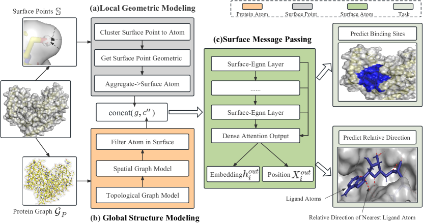
Figure 2. An illustration of the scheme of our EquiPocket framework.

2. Related Work

2.1. Binding Site Prediction

Computational Methods. The computational methods for binding site prediction include geometry-based (Levitt and Banaszak, 1992; Hendlich et al., 1997; Weisel et al., 2007; Le Guilloux et al., 2009; Chen et al., 2011; Dias et al., 2017), probe- and energy-based (Laskowski, 1995; Laurie and Jackson, 2005; Ngan et al., 2012) and template-based (Brylinski and Skolnick, 2008; Toti et al., 2018) methods: 1) Since most ligand binding sites occur on the 3D structure, geometry-based methods (POCKET (Levitt and Banaszak, 1992), CriticalFinder (Dias et al., 2017), LigSite (Hendlich et al., 1997), Fpocket (Le Guilloux et al., 2009), etc. ) are designed to identify these hollow spaces and then rank them using the expert design geometric features. 2) Probe-based methods (SURFNET  (Laskowski, 1995), Q-SiteFinder (Laurie and Jackson, 2005), etc. (Faller et al., 2015)), also known as energy-based methods, calculate the energy resulting from the interaction between protein atoms and a small-molecule probe, whose value dictates the existence of binding sites. 3)Template-based methods (FINDSITE (Brylinski and Skolnick, 2008), LIBRA (Toti et al., 2018), etc.) are mainly to compare the required query protein with the published protein structure database to identify the binding sites.

Traditional Learning-based Methods. PRANK (Krivák and Hoksza, 2015) is a learning-based method that employs the traditional machine learning algorithm random forest(RF) (Belgiu and Drăguţ, 2016). Based on the pocket points and chemical properties from Fpocket (Le Guilloux et al., 2009) and Concavity (Chen et al., 2011), this method measures the ”ligandibility” as the binding ability of a candidate pocket using the RF model. However, those methods require the manual extraction of numerous features with limit upgrading.

CNN-based Methods. Over the last few years, deep learning has surpassed far more traditional ML methods in many domains. For binding site prediction task, many researchers (Jiménez et al., 2017; Stepniewska-Dziubinska et al., 2020; Mylonas et al., 2021; Kandel et al., 2021; Aggarwal et al., 2021) regard a protein as a 3D image, and model this task as a computer vision problem. DeepSite (Jiménez et al., 2017) is the first attempt to employ the CNN architecture for binding site prediction, which like P2Rank (Krivák and Hoksza, 2018) treats this task as a binary classification problem and converts a protein to 3D voxelized grids. The methods FRSite (Jiang et al., 2019) and Kalasanty (Stepniewska-Dziubinska et al., 2020) adhere to the principle of deepsite, but the former regards this task as an object detection problem, and the latter regards this task as a semantic segmentation task. Deeppocket (Aggarwal et al., 2021) is a method similar to p2rank, but implements a CNN-based segmentation model as the scoring function in order to more precisely locate the the binding sites. The recent CNN-based method DeepSurf (Mylonas et al., 2021) constructs a local 3D grid and updates the 3D-CNN architecture to mitigate the detrimental effects of protein rotation.

2.2. Graph Neural Networks for Molecule Modeling

There are multi-level information in molecules including atom info, chemical bonds, spatial structure, physical constraints, etc. Numerous researchers view molecules as topological structures and apply topological-based GNN models (like graph2vec (Gonczarek et al., 2016), GAT (Velikovi et al., 2017), GCN (Kip and Welling, 2016), GCN2 (Chen et al., 2020), GIN (Xu et al., 2018) and etc. (Sun et al., 2019)) to extract the chemical info, which achieve positive outcomes. With the accumulation of structure data for molecules, spatial-based graph models  (DimeNet (Klicpera et al., 2020b) , DimeNet++ (Klicpera et al., 2020a), SphereNet (Liu et al., 2021), SchNet (Schütt et al., 2017), Egnn (Satorras et al., 2021b),  (Huang et al., 2022),  (Han et al., 2022) and etc.) are proposed for molecule task which aggregates spatial and topological information. However, these models may not be adequate for macro-molecules due to their high calculation and resource requirements.

3. Notations and Definitions

Protein Graph.

A protein such as the example in Figure 1(b) is denoted as a graph ${\mathcal{G}}_{P}=({\mathcal{V}}_{P},{\mathcal{E}}_{C},{\mathcal{E}}_{D})$, where ${\mathcal{V}}_{P}=\left\{v_{0},...,v_{N}\right\}$ forms the set of $N$ atoms, ${\mathcal{E}}_{C}$ represents the chemical-bond edges, and ${\mathcal{E}}_{D}$ collects the spatial edges between any two atoms if their spatial distance is less than a cutoff $\theta>0$. In particular, each node (i.e. atom) is associated with a feature $({\bm{x}}_{i},{\bm{c}}_{i})$, where ${\bm{x}}_{i}\in\mathbb{R}^{3}$ denotes the 3D coordinates and ${\bm{c}}_{i}\in\mathbb{R}^{5}$ is the chemical feature.

Surface Point Set.

The surface geometry of a protein is of crucial interest for binding site detection. Here we define the set of surface points, by ${\mathbb{S}}=\left\{s_{0},...,s_{M}\right\}$, $M\gg N$. Each surface point $s_{i}$ is NOT necessarily an atom of the protein, and it corresponds to $({\bm{x}}_{i},p_{i})$, where ${\bm{x}}_{i}\in\mathbb{R}^{3}$ represents the 3D coordinates of $s_{i}$ and $p_{i}\in{\mathcal{V}}_{P}$ indicates the index of the nearest protein atom in ${\mathcal{V}}_{P}$ to $s_{i}$. We employ the open source MSMS (Sanner et al., 1996) to derive surface points.

Protein Surface Graph.

By referring to the surface points defined above, we collect all the nearest protein atoms $p_{i}$ of the surface points, giving rise to the surface graph ${\mathcal{G}}_{S}=({\mathcal{V}}_{S},{\mathcal{E}}_{S})$, and clearly ${\mathcal{G}}_{S}\subseteq{\mathcal{G}}_{P}$. We call the atoms in the surface graph as surface atoms, which are distinguished from surface points defined in the last paragraph. Notably, the edges of the surface graph, i.e. , ${\mathcal{E}}_{S}$ is only composed of spatial edges from ${\mathcal{E}}_{D}$, since those chemical edges are mostly broken among the extracted atoms.

Equivariance and Invariance.

In 3D space, the symmetry of the physical laws requires the detection model to be equivariant with respect to arbitrary coordinate systems (Han et al., 2022). In form, suppose ${{\bm{X}}}$ to be 3D geometric vectors (positions, velocities, etc) that are steerable by E(3) group (rotations/translations/reflections), and ${\bm{h}}$ non-steerable features. The function $f$ is E($3$)-equivariant, if for any transformation $g\in\text{E}(3)$, $f(g\cdot{{\bm{X}}},{\bm{h}})=g\cdot f({{\bm{X}}},{\bm{h}})$, $\forall{{\bm{X}}}\in{\mathbb{R}}^{3\times m},{\bm{h}}\in{\mathbb{R}}^{d}$. Similarly, $f$ is invariant if $f(g\cdot{{\bm{X}}},{\bm{h}})=f({{\bm{X}}},{\bm{h}})$. The group action $\cdot$ is instantiated as $g\cdot{{\bm{X}}}:={{\bm{X}}}+{\bm{b}}$ for translation ${\bm{b}}\in\mathbb{R}^{3}$ and $g\cdot{{\bm{X}}}(t):={\bm{O}}{{\bm{X}}}$ for rotation/reflection ${\bm{O}}\in\mathbb{R}^{3\times 3}$.

Problem Statement.

Given a protein ${\mathcal{G}}_{P}$ and its surface points ${\mathbb{S}}$, as well as the constructed surface graph ${\mathcal{G}}_{S}$, our goal is to learn an E(3)-invariant model $f({\mathcal{G}}_{P},{\mathbb{S}},{\mathcal{G}}_{S})$ to predict the atoms of the binding site: ${\mathcal{V}}_{B}\subseteq{\mathcal{V}}_{P}$.

4. The proposed methodology

Figure 2 illustrates the overall framework of our EquiPocket, which consists of three modules: the local geometric modeling module § 4.1 that focuses on extracting the geometric information of each surface atom, the global structure modeling module § 4.2 to characterize both the chemical and spatial structures of the protein, and the surface message passing module § 4.3 which concentrates on capturing the entire surface geometry based on the extracted information by the two former modules. The training losses are also presented. We defer the pseudo codes of EquiPocket to Appendix 1.

4.1. Local Geometric Modeling Module

This subsection presents how to extract the local geometric information of the protein surface ${\mathcal{G}}_{S}$, with the help of surface points ${\mathbb{S}}$. The local geometry of each protein atom closely determines if the region nearby is appropriate or not to become part of binding sites. We adopt the surrounding surface points of each protein surface atom to describe the local geometry.

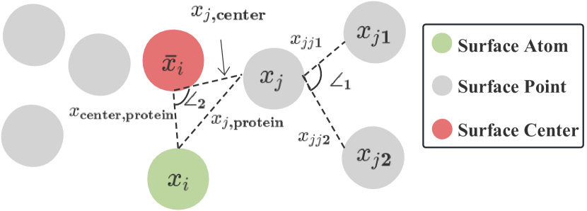
Figure 3. An illustration of local geometric features.

To be specific, for every surface atom $i\in{\mathcal{V}}_{S}$, its surrounding surface points are returned by a subset of ${\mathbb{S}}$, namely, ${\mathbb{S}}_{i}=\{s_{j}=({\bm{x}}_{j},p_{j})\in{\mathbb{S}}\mid p_{j}=i\}$, where $p_{j}$, as defined before, indicates the nearest protein atom. We now construct the geometric information based on ${\mathbb{S}}_{i}$. We denote the center/mean of all 3D coordinates in ${\mathbb{S}}_{i}$ as $\bar{{\bm{x}}}_{i}$. For each surrounding surface point $s_{j}\in{\mathbb{S}}_{i}$, we first search its two nearest surface points from ${\mathbb{S}}$ as $s_{j_{1}}$ and $s_{j_{2}}$, and then calculate the following relative position vectors:

(1) $$\begin{aligned} \left\{\begin{array}[]{l}{\bm{x}}_{jj_{1}}={\bm{x}}_{j}-{\bm{x}}_{j_{1}},\\ {\bm{x}}_{jj_{2}}={\bm{x}}_{j}-{\bm{x}}_{j_{2}},\\ {\bm{x}}_{j,\text{center}}={\bm{x}}_{j}-\bar{{\bm{x}}}_{i},\\ {\bm{x}}_{j,\text{protein}}={\bm{x}}_{j}-{\bm{x}}_{i},\\ {\bm{x}}_{\text{center},\text{protein}}=\bar{{\bm{x}}}_{i}-{\bm{x}}_{i}.\end{array}\right.\end{aligned}$$

We further derive the following scalars upon Eq. 1:

(2) $$\begin{aligned} &{\bm{g}}(s_{j})\coloneqq[\|{\bm{x}}_{jj_{1}}\|_{2},\|{\bm{x}}_{jj_{2}}\|_{2},\angle_{1},\\ &\|{\bm{x}}_{j,\text{center}}\|_{2},\|{\bm{x}}_{j,\text{protein}}\|_{2},\|{\bm{x}}_{\text{protein},\text{center}}\|_{2},\angle_{2}],\end{aligned}$$

where the angels are computed by $\angle_{1}=\frac{{\bm{x}}_{jj_{1}}\cdot{\bm{x}}_{jj_{2}}}{\|{\bm{x}}_{jj_{1}}\|_{2}\|{\bm{x}}_{jj_{2}}\|_{2}}$ and $\angle_{2}=\frac{{\bm{x}}_{j,\text{center}}\cdot{\bm{x}}_{\text{center},\text{protein}}}{\|{\bm{x}}_{j,\text{center}}\|_{2}\|{\bm{x}}_{\text{center},\text{protein}}\|_{2}}$; here the operator $\cdot$ defines the inner-product between two vectors. Basically, as displayed in Figure 3, the first three quantities in ${\bm{g}}(s_{j})$ depict how the nearby surface points are arranged around $s_{j}$, and the last four ones describe where $s_{j}$ is located within the global region of ${\mathbb{S}}_{i}$.

We aggregate the geometric information ${\bm{g}}(s_{j})$ over all surface points in ${\mathbb{S}}_{i}$ and obtain a readout descriptor for surface atom $i$ as

(3) $$\begin{aligned} {\bm{g}}_{i}=&[\text{Pooling}(\{\text{MLP}({\bm{g}}(s_{j}))\}_{s_{j}\in{\mathbb{S}}_{i}}),\\ &\quad\text{MLP}(\text{Pooling}\{({\bm{g}}(s_{j}))\}_{s_{j}\in{\mathbb{S}}_{i}})]\end{aligned}$$

Here, MLP denotes multi-layer perceptron, and the function Pooling is implemented as a concatenation of mean pooling and max pooling throughout our experiments. The front part in Eq. 3 is used to gather local geometric features, while the latter part attempts to compute the global size of surrounding surface points. Notably, the geometric descriptor ${\bm{g}}_{i}$ is E(3)-invariant.

4.2. Global Structure Modeling Module

This module aims at processing the information of the whole protein ${\mathcal{G}}_{P}$, including atom type, chemical bonds, relevant spatial positions, etc. Although the binding pocket is majorly comprised of surface atoms, the global structure of the protein in general influences how the ligand is interacted with and how the pocket is formulated, which should be modeled. We fulfil this purpose via two concatenated processes: chemical-graph modeling and spatial-graph modeling.

The chemical-graph modeling process copes with the chemical features $\{{\bm{c}}_{i}\}_{i\in{\mathcal{V}}_{P}}$ and the chemical interactions ${\mathcal{E}}_{C}$ of the protein graph. For each atom in the protein, its chemical type, the numbers of electrons around, and the chemical bonds connected to other atoms are important clues to identify the interaction between the protein and the ligand (Zhang et al., 2022). We employ typical GNNs (Kipf and Welling, 2016; Velikovi et al., 2017; Sabrina et al., 2018) to distill this type of information. Formally, we proceed:

(4) $$\{{\bm{c}}^{\prime}_{i}\}_{i\in{\mathcal{V}}_{P}}=\text{GNN}(\{{\bm{c}}_{i}\}_{i\in{\mathcal{V}}_{P}},{\mathcal{E}}_{C}),$$

where ${\bm{c}}^{\prime}_{i}$ is the updated chemical feature for atom $v_{i}$. While various GNNs can be used in Eq. 4, here we implement GAT (Velikovi et al., 2017) given its desirable performance observed in our experiments.

The spatial-graph modeling process further involves the 3D coordinates $\{{\bm{x}}_{i}\}_{i\in{\mathcal{V}}_{P}}$ to better depict the spatial interactions ${\mathcal{E}}_{D}$ within the protein. Different from chemical features ${\bm{c}}^{\prime}_{i}$, the 3D coordinates provide the spatial position of each atom and reflect the pair-wise distances in 3D space, which is helpful for physical interaction modeling. We leverage EGNN (Satorras et al., 2021b) as it conforms to E(3) equivariance/invariance and achieves promising performance on modeling spatial graphs. Specifically, we process EGNN as follows:

(5) $$\{{\bm{c}}^{\prime\prime}_{i}\}_{i\in{\mathcal{V}}_{P}}=\text{EGNN}(\{{\bm{x}}_{i},{\bm{c}}^{\prime}_{i}\}_{i\in{\mathcal{V}}_{P}},{\mathcal{E}}_{D}).$$

Here, we only reserve the invariant output (i.e. , ${\bm{c}}^{\prime\prime}_{i}$) and have discarded the equivariant output (e.g. updated 3D coordinates) of EGNN, since the goal of this module is to provide invariant features. We select the updated features of the surface atoms ${\mathcal{V}}_{S}$, which will be fed into the module in § 4.3.

4.3. Surface Message Passing Module.

Given the local geometric features $\{{\bm{g}}_{i}\}_{i\in{\mathcal{V}}_{S}}$ from § 4.1, and the globally-encoded features of the surface atoms $\{{\bm{c}}^{\prime\prime}_{i}\}_{i\in{\mathcal{V}}_{S}}$ from § 4.2, the module in this subsection carries out equivariant message passing on the surface graph ${\mathcal{G}}_{S}$ to renew the entire features of the protein surface. We mainly focus on the surface atoms here, because firstly the surface atoms are more relevant to the binding sites than the interior atoms, and secondly the features $\{{\bm{c}}^{\prime\prime}_{i}\}_{i\in{\mathcal{V}}_{S}}$ that are considered as the input have somehow encoded the information of the interior structure via the processes in 4.2.

Surface-EGNN. During the $l$-th layer message passing, each node is associated with an invariant feature ${\bm{h}}_{i}^{(l)}\in\mathbb{R}^{m_{l}}$ and an equivariant double-channel matrix ${\bm{X}}_{i}^{(l)}\in\mathbb{R}^{3\times 2}$. We first concatenate ${\bm{c}}^{\prime\prime}_{i}$ with ${\bm{g}}_{i}$ as the initial invariant feature:

(6) $${\bm{h}}^{(0)}_{i}=[{\bm{c}}^{\prime\prime}_{i},{\bm{g}}_{i}].$$

The equivariant matrix ${\bm{X}}_{i}^{(0)}$ is initialized by the 3D coordinates of the atom and the center of its surrounding surface points, that is,

(7) $${\bm{X}}^{(0)}_{i}=[{\bm{x}}_{i},\bar{{\bm{x}}}_{i}].$$

We update ${\bm{h}}_{i}^{(l)}\in\mathbb{R}^{d_{l}}$ and ${\bm{X}}_{i}^{(l)}\in\mathbb{R}^{3\times 2}$ synchronously to unveil both the topological and geometrical patterns. Inspired from EGNN (Satorras et al., 2021b) and its multi-channel version GMN (Huang et al., 2022), we formulate the $l$-th layer for each surface atom $i\in{\mathcal{V}}_{S}$ as:

(8) $${\bm{m}}_{ij} =\phi_{m}\left({\bm{h}}_{i}^{(l)},{\bm{h}}_{j}^{(l)},f_{x}({\bm{X}}_{i}^{(l)},{\bm{X}}_{j}^{(l)}),e_{ij}\right),$$

(9) $${\bm{h}}_{i}^{(l+1)} =\phi_{h}\left({\bm{h}}_{i}^{(l)},\sum\nolimits_{j\in{\mathbb{N}}(i)}{\bm{m}}_{ij}\right),$$

(10) $${\bm{X}}_{i}^{(l+1)} ={\bm{X}}_{i}^{(l)}+\frac{1}{|{\mathbb{N}}(i)|}\sum\nolimits_{j\in{\mathcal{N}}(i)}({\bm{x}}_{i}^{(l)}-{\bm{x}}_{j}^{(l)})\phi_{x}({\bm{m}}_{ij}),$$

where the functions $\phi_{m},\phi_{h},\phi_{x}$ are all MLPs, ${\mathbb{N}}(i)$ denotes the neighbors of node $i$ in terms of the spatial edges ${\mathcal{E}}_{d}$, $|\cdot|$ counts the size of the input set, and the invariant message ${\bm{m}}_{ij}$ from node $j$ to $i$ is employed to update the invariant feature ${\bm{h}}_{i}^{(l+1)}$ via $\phi_{h}$ and the equivariant matrix ${\bm{X}}_{i}^{(l+1)}$ via the aggregation of the relative position ${\bm{x}}_{i}^{(l)}-{\bm{x}}_{j}^{(l)}$ multiplied with $\phi_{x}$.

As a core operator in the message passing above, the function $f_{x}({\bm{X}}_{i},{\bm{X}}_{j})$ is defined as follows:

(11) $$f_{x}({\bm{X}}_{i},{\bm{X}}_{j})\coloneqq[\|{\bm{x}}_{ij}\|_{2},\|{\bm{x}}_{ci}\|_{2},\|{\bm{x}}_{cj}\|_{2},\angle_{ci,ij},\angle_{cj,ij},\angle_{ci,cj}],$$

where, the relative positions are given by ${\bm{x}}_{ij}={\bm{x}}_{i}-{\bm{x}}_{j}$, ${\bm{x}}_{ci}=\bar{{\bm{x}}}_{i}-{\bm{x}}_{i}$ and ${\bm{x}}_{cj}=\bar{{\bm{x}}}_{j}-{\bm{x}}_{j}$; the angles $\angle_{ci,ij},\angle_{cj,ij},\angle_{ci,cj}$ are defined as the inner-products of the corresponding vectors denoted in the subscripts, e.g. , $\angle_{ci,ij}=\frac{{\bm{x}}_{ci}\cdot{\bm{x}}_{ij}}{\|{\bm{x}}_{ci}\|_{2}\|{\bm{x}}_{ij}\|_{2}}$. Through the design in Eq. 11, $f_{x}({\bm{X}}_{i},{\bm{X}}_{j})$ elaborates the critical information (including relative distances and angles) around the four points: ${\bm{x}}_{i},\bar{{\bm{x}}}_{i},{\bm{x}}_{j},\bar{{\bm{x}}}_{j}$, which largely characterizes the geometrical interaction between the two input matrices. Nicely, $f_{x}({\bm{X}}_{i},{\bm{X}}_{j})$ is invariant, ensuring the equivariance of the proposed Surface-EGNN.

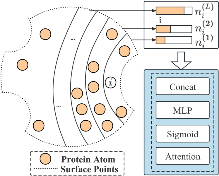
Figure 4. An illustration of Dense Attention in a Protein.

Dense Attention Output Layer. Conventionally, we can apply the output of the final layer, i.e. , $({\bm{h}}_{i}^{(L)},{\bm{X}}_{i}^{(L)})$ to estimate the binding site. Nevertheless, such flat output overlooks the discrepancy of size and shape between different proteins. As showed in Figure 5, for small or densely-connected proteins, the receptive field of each node will easily cover most nodes after a small number of message-passing layers, and excessive message passing will lead to over-smoothing (Huang et al., 2020) that will incurs performance detriment. For large or sparsely-connected proteins, on the contrary, insufficient message passing can hardly attain the receptive field with a desirable scope, which will also decrease the performance. It thus requires us to develop an adaptive mechanism to balance the message passing scope between different proteins. We propose the dense attention output layer to achieve this goal.

Intuitively, for each target atom, the spatial distribution of the neighbors is able to reflect the density of the spatial connections around. This motivates us to calculate the proportion of the atoms with different distance ranges. As $\theta$ is the cutoff to create the spatial graph, we use it as the distance unit. We compute by:

(12) $$n_{i}^{(l)}=\frac{|\{j\in{\mathcal{V}}_{P}\mid 0\leq\|{\bm{x}}_{i}-{\bm{x}}_{j}\|_{2}<l\theta\}|}{N_{P}},$$

where, the proportion is evaluated within the distance range $[0,l\theta]$, $N_{P}=|{\mathcal{V}}_{P}|$, and the neighbor hop $l\in{\mathbb{Z}}^{+}$. We collect the proportions of all hops from 0 to $L$, yielding the proportion vector ${\bm{n}}_{i}=[n_{i}^{(0)},n_{i}^{(1)},\cdots,n_{i}^{(L)},N_{P}]\in\mathbb{R}^{L+2}$ with $N_{P}$ plus to emphasize the total number of the protein atoms. Clearly, ${\bm{n}}_{i}$ contains rich information of the spatial density, and we apply it to determine the importance of different layers, by producing the attention as:

(13) $${\bm{a}}_{i}=\text{Sigmoid}(\phi_{a}({\bm{n}}_{i})).$$

Here, $\phi_{a}$ is an MLP with the number of output channels as $L+1$, the Sigmoid function is applied for each channel, implying that ${\bm{a}}_{i}\in(0,1)^{L+1}$. We then multiply the hidden feature of the corresponding layer with each channel of the attention vector, and concatenate them into a vector:

(14) $${\bm{h}}_{i}^{\text{out}}=\text{Concat}(a_{i0}{\bm{h}}_{i}^{(0)},...,a_{iL}{\bm{h}}_{i}^{(L)}),$$

where $a_{il}$ is the $l$-th channel of ${\bm{a}}_{i}$. By making use of Eq. 14, the learnable attentions enable the model to adaptively balance the importance of different layers for different input proteins. We will illustrate the benefit of the proposed strategy in our experiments. As for the coordinates, we simply compute the mean of all layers to retain translation equivariance:

(15) $${\bm{X}}_{i}^{\text{out}}=\frac{1}{L+1}\sum_{l=0}^{L}{\bm{X}}_{i}^{(l)}.$$

4.4. Optimization Objective

We set $y_{i}=1$ if a surface atom $i$ is within 4Å to any ligand atom (Mylonas et al., 2021) . We predict the probability $\hat{y_{i}}$ of being a part of binding site according its dense embedding $h_{i}$.

(16) $$\hat{y_{i}}=\textbf{Sigmoid}(\text{MLP}({\bm{h}}_{i}^{\text{out}})).$$

Following (Jiménez et al., 2017; Kandel et al., 2021), Dice loss is used:

(17) $$\mathcal{L}_{b}=1-\frac{2\cdot\sum(\hat{y}_{i}\cdot y_{i})}{\sum(\hat{y}_{i})+\sum(y_{i})+\epsilon},$$

where $\epsilon>0$ is a small value to maintain numeric stability.

Predict the relative direction of nearest ligand atom. Beyond the CNN-based methods, our EquiPocket is an E(3)-equivariant model, which can not only output the embedding ${\bm{h}}_{i}^{\text{out}}$ but also the coordinate matrix ${\bm{X}}_{i}^{\text{out}}$ (with initial position vector ${\bm{x}}_{i}$). We further leverage the position vector to predict the relative direction ${\bm{d}}_{i}$ of its nearest ligand atom (with position vector ${\bm{m}}_{i}$), in order to enhance our framework to gather local geometric features.

(18) $${\bm{d}}_{i}=\frac{{\bm{m}}_{i}-{\bm{x}}_{i}}{\|{\bm{m}}_{i}-{\bm{x}}_{i}\|_{2}}, \hat{{\bm{d}}}_{i}=\frac{{\bm{x}}_{i}^{\text{out}}-{\bm{x}}_{i}}{\|{\bm{x}}_{i}^{\text{out}}-{\bm{x}}_{i}\|_{2}}.$$

The cosine loss function is used for the direction loss $\mathcal{L}_{d}$:

(19) $$\mathcal{L}_{d}=\sum(1-\text{cos}(\hat{{\bm{d}}}_{i},{\bm{d}}_{i})).$$

The eventual loss is $\mathcal{L}=\mathcal{L}_{b}+\mathcal{L}_{d}$. We train the parameters of all the three modules end to end.

5. Experiments

In this section, we will conduct experiments on multiple datasets to evaluate the performance of our framework in comparison to baseline methods and investigate the following tasks:

• Task 1. Can our framework’s performance match or surpass that of existing methods?

• Task 2. Can different modules of our framework bring significant improvement for binding site prediction?

• Task 3. Can our framework mitigate the detrimental effects of the data distribution shift?

• Task 4. How do the hyperparameters (the cutoff $\theta$ and depth of surface-egnn) affect the performance and computational cost?

5.1. Experimental Settings

5.1.1. Dataset

We conduct experiments based on the following datasets:

• scPDB (Desaphy et al., 2015) is the famous dataset for binding site prediction, which contains the protein structure, ligand structure, and 3D cavity structure generated by VolSite (Da Silva et al., 2018). The 2017 release of scPDB is used for training and cross-validation of our framework, which contains 17,594 structures, 16,034 entries, 4,782 proteins, and 6,326 ligands.

• PDBbind  (Wang et al., 2004) is a well-known and commonly used dataset for the research of protein-ligand complex. It contains the 3D structures of proteins, ligands, binding sites, and accurate binding affinity results determined in the laboratory. We use the release of v2020, which consists of two parts: general set (14, 127 complexes) and refined set (5,316 complexes). The general set contains all protein-ligand complexes. The refined set contains better-quality compounds selected from the general set, which is used for the test in our experiments.

• COACH 420 and HOLO4K are two test datasets for the binding site prediction, which are first introduced by (Krivák and Hoksza, 2018). Consistent with (Krivák and Hoksza, 2018; Mylonas et al., 2021; Aggarwal et al., 2021), we use the mlig subsets of each dataset for evaluation, which contain the relevant ligands for binding site prediction.

Data Distribution Shift. As depicted in the Figure 5 and Table 1 that after data processing, there is a significant gap in protein size and protein distribution between the training dataset (scPDB) and the test dataset (COACH420, HOLO4k, PDBbind). The number of atoms within a protein ranges from hundreds to tens of thousands. As for protein distribution in datasets, scPDB has the longest average structure, followed by HOLO4k and PDBbind, with COACH420 having the shortest average protein structure. This fact will hurt model learning and generalization, as discussed in § 5.2.3.

5.1.2. Target of Binding Sites

The CNN-based methods (Jiménez et al., 2017; Aggarwal et al., 2021; Stepniewska-Dziubinska et al., 2020) label the subgrid as positive if its geometric center is closer than 4Å to the binding sites geometric center. In our experiment, consistent with (Mylonas et al., 2021), we set the protein atoms within 4Å of any ligand atom as positive and negative otherwise. After obtaining the probability that an atom is a candidate binding site, we use the mean-shift algorithm (Comaniciu and Meer, 2002) to predict the binding site center, which can determine the number of clusters on its own (details in Appendix A.2.4).

Table 1. Summary of Dataset

DataSet	Average
	Atom Num	Atom in Surface	Surface Points	Target Atoms
scPDB	4205	2317	24010	47
COACH420	2123	1217	12325	58
HOLO4k	3845	2052	20023	106
PDBbind	3104	1677	17357	37

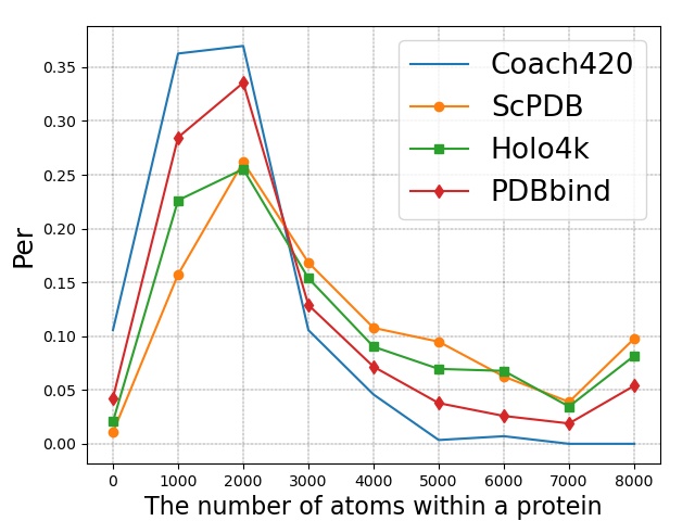
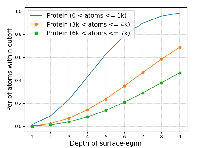
Figure 5. The protein distribution of datasets and spatial distribution of atom neighbors

5.1.3. Data Preparation

Table 2. Experimental and ablation results of baseline models and our framework.^a

Methods	Type	Param	Failure	COACH420		HOLO4K		PDBbind2020
		(M)	Rate $\downarrow$	DCC$\uparrow$	DCA$\uparrow$	DCC$\uparrow$	DCA$\uparrow$	DCC$\uparrow$	DCA$\uparrow$
Fpocketb	Geometric-based	$\textbackslash$	0.000	0.228	0.444	0.192	0.457	0.253	0.371
DeepSiteb	3D-CNN	1.00	$\textbackslash$	$\textbackslash$	0.564	$\textbackslash$	0.456	$\textbackslash$	$\textbackslash$
Kalasantyb		70.64	0.120	0.335	0.636	0.244	0.515	0.416	0.625
DeepSurfb		33.06	0.054	0.386	0.658	0.289	0.635	0.510	0.708
GAT		0.03	0.11	0.039(0.005)	0.130(0.009)	0.036(0.003)	0.110(0.010)	0.032(0.001)	0.088(0.011)
GCN	Topological	0.06	0.163	0.049(0.001)	0.139(0.010)	0.044(0.003)	0.174(0.003)	0.018(0.001)	0.070(0.002)
GAT + GCN	Graph	0.08	0.31	0.036(0.009)	0.131(0.021)	0.042(0.003)	0.152(0.020)	0.022(0.008)	0.074(0.007)
GCN2		0.11	0.466	0.042(0.098)	0.131(0.017)	0.051(0.004)	0.163(0.008)	0.023(0.007)	0.089(0.013)
SchNet	Spatial	0.49	0.14	0.168(0.019)	0.444(0.020)	0.192(0.005)	0.501(0.004)	0.263(0.003)	0.457(0.004)
Egnn	Graph	0.41	0.270	0.156(0.017)	0.361(0.020)	0.127(0.005)	0.406(0.004)	0.143(0.007)	0.302(0.006)
EquiPocket-L	Ours	0.15	0.552	0.070(0.009)	0.171(0.008)	0.044(0.004)	0.138(0.006)	0.051(0.003)	0.132(0.009)
EquiPocket-G		0.42	0.292	0.159(0.016)	0.373(0.021)	0.129(0.005)	0.411(0.005)	0.145(0.007)	0.311(0.007)
EquiPocket-LG		0.50	0.220	0.212(0.016)	0.443(0.011)	0.183(0.004)	0.502(0.008)	0.274(0.004)	0.462(0.005)
EquiPocket		1.70	0.051	0.423(0.014)	0.656(0.007)	0.337(0.006)	0.662(0.007)	0.545(0.010)	0.721(0.004)

• The standard deviation of each index is indicated in brackets. The result of 5-fold for EquiPocket is shown in Appendix A.2.5.

• We use their published pre-train models or published result, details in Appendix A.2.3.

We perform the following four processing steps: i) Cluster the structures in scPDB by their Uniprot IDs, and select the longest sequenced protein structures from every cluster as the train data (Kandel et al., 2021). Finally, 5,372 structures are selected out. ii) Split proteins and ligands for the structures in COACH420 and HOLO4k, according to the research (Krivák and Hoksza, 2018) . iii) Clean protein by removing the solvent, hydrogens atoms. Using MSMS (Sanner et al., 1996) to generate the solvent-accessible surface of a protein. iv) Read the protein file by RDKIT (Tosco et al., 2014), and extract the atom and chemical bond features. Remove the error structures.

5.1.4. Evaluation Metrics

DCC is the distance between the predicted binding site center and the true binding site center. DCA is the shortest distance between the predicted binding site center and any atom of the ligand. The samples with DCC(DCA) less than the threshold are considered successful. The samples without any binding site center are considered failures. Consistent with (Jiménez et al., 2017; Mylonas et al., 2021; Aggarwal et al., 2021; Stepniewska-Dziubinska et al., 2020), threshold is set to 4 Å. We use Success Rate and Failure Rate to evaluate experimental performance.

(20) $$\text{Success Rate(DCC)}=\frac{1(\{\text{Predicted sites}|\text{DCC}<\text{threshold}\})}{1(\{\text{True sites}\})},$$

$$\text{Success Rate(DCA)}=\frac{1(\{\text{Predicted sites}|\text{DCA}<\text{threshold}\})}{1(\{\text{True sites}\})},$$

$$\text{Failure Rate}=\frac{1(\{\text{Protein}|1(\text{predicted binding center})=0\})}{1(\{\text{Protein}\})},$$

where $1(\cdot)$ represents the cardinality of a set. After ranking the predicted binding sites, we take the same number with the true binding sites to calculate the success rate.

5.1.5. EquiPocket Framework

We implement our EquiPocket framework based on (GAT (Velikovi et al., 2017)+EGNN (Satorras et al., 2021b)) as our global structure modeling module. The cutoff $\theta$ and depth in our surface-egnn model are set to 6 and 4 .

To indicate the EquiPocket Framework with different modules, we adopt the following symbol as follows: i) EquiPocket-L: Only contain the local geometric modeling module. ii) EquiPocket-G: Only contain the global structure modeling module. iii) EquiPocket-LG: Only contain both the local geometric and global structure modeling modules. iii) EquiPocket: Contain all the modules.

5.1.6. Baseline Models

We compare our framework with the following models: 1) geometric-based method(Fpocket (Le Guilloux et al., 2009)), 2) CNN-based methods (DeepSite (Jiménez et al., 2017), Kalasanty (Stepniewska-Dziubinska et al., 2020) and DeepSurf (Mylonas et al., 2021)), 3) topological graph-based models (GAT (Velikovi et al., 2017), GCN (Kip and Welling, 2016) and GCN2 (Chen et al., 2020)), 4) spatial graph-based models (SchNet (Schütt et al., 2017), EGNN (Satorras et al., 2021a)).

5.1.7. Environment and Parameter.

We implement our EquiPocket framework in PyTorch Geometric, all the experiments are conducted on a machine with an NVIDIA A100 GPU (80GB memory). We take 5-fold cross validation on training data scPDB and use valid loss to save checkpoint. The batch size is set to 8. For baseline models and models in global structure modeling module of EquiPocket, we use them suggested settings to get optimal performance. More details and related resources for our experiments can be found in Appendix A.2.2.

5.2. Result analysis

5.2.1. Model Comparison

In Table 2, we compared our EquiPocket framework with baseline methods mentioned above. As can be observed, the performance of the computational method Fpocket is inferior, with no failure rate, since it simply employs the geometric feature of a protein. The performance of CNN-based methods is much superior to that of the conventional method, with DCC and DCA metrics improving by more than 50 percent but requiring enormous parameter values and computing resources. However, these two early methods DeepSite and Kalasanty are hampered by data distribution shift (Issue 4) and their inability to process big proteins, which may fail prediction. The recently proposed method Deepsurf employs the local-grid concept to handle any size of proteins, although CNN architecture also still results in inevitable failures.

For graph models, the poor performance of topological-graph models (GCN, GAT, GCN2) is primarily due to the fact that they only consider atom attributes and chemical bond information, ignoring the spatial structure in a protein. The performance of spatial-graph models is generally better than that of topological-graph models. EGNN model utilizes not only the properties of atoms but also their relative and absolute spatial positions, resulting in a better effect. SchNet merely updates the information of atoms based on the relative distance of atoms. We attempt to execute the Dimenet++ (Klicpera et al., 2020a), which uses the angle info between atoms and atoms, but it requires too many computing resources, resulting in an OOM (Out Of Memory) error. However, the performance of the spatial-graph model is worse than that of the CNN-based and geometric-based methods because the former cannot obtain enough geometric features (Issue 3) and cannot address the data distribution shift (Issue 4).

As the above results indicate, geometric info of protein surface and multi-level structure info in a protein is essential for binding site prediction. In addition, it reflects the limitations of the current GNN models, where it is difficult to collect sufficient geometric information from the protein surface or the calculation resources are too large to apply to macromolecular systems like proteins. Consequently, our EquiPocket framework is not only able to update chemical and spatial information from an atomic perspective but also able to effectively collect geometric information without excessive computing expense, resulting in a 10-20% increase in effect over previous results. Case study based on different methods is showed in Appendix 5.2.5.

5.2.2. Ablation Study

As shown in Table 2, we conduct ablation experiments on our EquiPocket framework with different modules.

Local Geometric Modeling Module. This module is used to extract the geometric features of protein atoms from their nearest surface points. EquiPocket-G consists solely of this module, and the performance is negligible. There are two primary causes for this result. First, geometric information can only determine part of the binding sites. Second, it can only reflect the geometric features over a relatively small distance and cannot cover an expansive area.

Global Structure Modeling Module. The primary purpose of this module is to extract information about the whole protein, such as atom type, chemical bonds, relevant spatial positions, etc. We implement EquiPocket-G based on (GAT + EGNN) models, which is E(3) equivariance/invariance and has a better effect than its predecessor, EquiPocket-L. In comparison, the value of DCC increased by about 10%, and DCA increased by about 20%. This demonstrates that structure information of the whole protein is necessary for binding site prediction. In addition, when the two modules are combined as the EquiPocket-LG, the prediction effect is significantly improved, proving the complementarity of surface geometric information and global structure information.

Surface Message Passing Module. In the previous model, EquiPocket-LG, information was extracted solely from atoms and their closest surface points. Nonetheless, the binding site is determined not only by the information of a single atom but also by the atoms surrounding it. Therefore, the surface message passing module is proposed to collect and update the atom’s features from its neighbors. After adding this module, the performance of EquiPocket has been significantly enhanced, DCC and DCA have increased by approximately 20% on average, and the failure rate has been significantly reduced. Through the addition of multiple modules, we address the Issue 3 and the performance of our framework eventually surpasses that of the existing SOTA method, demonstrating the efficacy of our framework design.

5.2.3. Data Distribution Shift

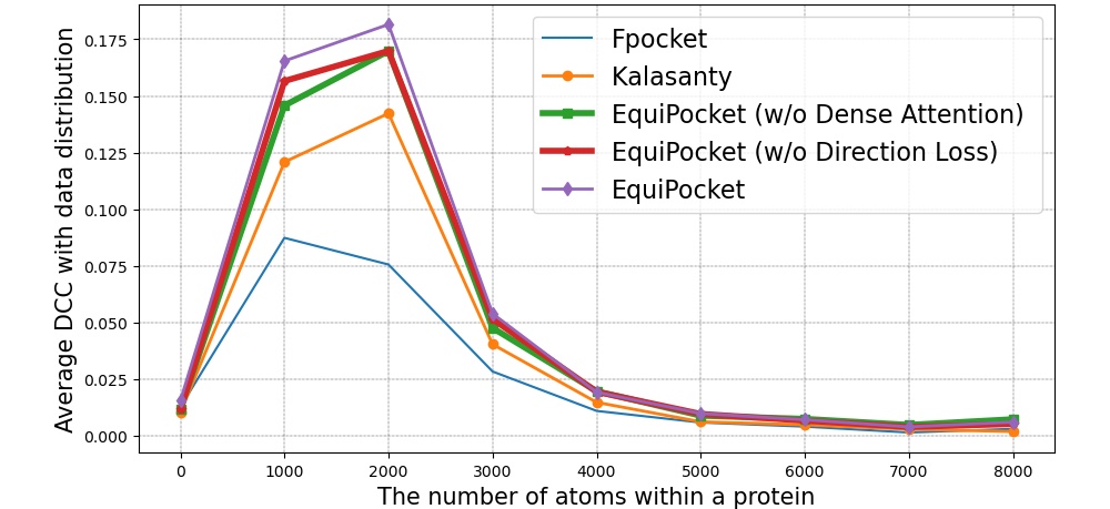
Figure 6. The performance of EquiPocket and baseline methods for proteins of various sizes.

As shown in Figure 6, we calculate the average DCC with the distribution of various sizes proteins. The geometric-based method Fpocket only utilizes the geometric features of a protein surface. Therefore, its performance is superior to that of most other methods for proteins with fewer than 1,000 atoms, but its prediction effect decreases significantly as the size of the protein increases. Kalasanty is a CNN-based and learn-based method. As the number of atoms in the protein varies, the prediction effect exhibits an increasing and then a decreasing trend, which is not only influenced by the size of the protein but also has a significant correlation with the dataset’s distribution. According to the train data (scPDB), the majority of proteins contain fewer than 2,000 protein atoms (as depicted in Figure 5). Consequently, the model’s parameters will be biased toward this protein size. In addition, for proteins with more than 8000 atoms, the prediction effect is not even as good as the geometric-based method. This is due to the fact that CNN methods typically restrict the protein space to 70Å * 70Å * 70Å, and for proteins larger than this size, the prediction frequently fails. For our EquiPocket framework, we do not need to cut the protein into grids, and we utilize both geometric information from the surface points and global structure information from the whole protein, so the performance for proteins of varying sizes is significantly superior to that of other methods.

Dense Attention. The Dense Attention is introduced in  § 4.3 to reduce the negative impact caused by the data distribution shift (Issue 4). As shown in 6, when the number of atoms contained in a protein is less than 3000, the result of the EquiPocket (w/o Dense Attention) is weaker than that of the original EquiPocket, whereas when the protein is larger, there is no significant distinction between the two models. It simply reflects the role of Dense Attention, which, by weighting the surface-egnn layer at different depths, mitigates the detrimental effect of the data distribution shift.

Direction Loss. Direction loss is a novel task designed to improve the extraction of local geometric features. The result of the EquiPocket (w/o Direction Loss) in Figure 6 demonstrates conclusively that the prediction performance of small proteins with fewer than 3,000 atoms is diminished in the absence of this task, which reveals the importance of the task.

5.2.4. Hyperparameters Analysis

In our EquiPocket framework, the cutoff $\theta$ and depth of surface-egnn are two crucial parameters that can impact performance and computational efficiency.

Cutoff $\theta$. We set the depth of surface-egnn to 4 and implement various cutoff values (2, 4, 6, 8, 10). Figure 7 indicates that when the cutoff is set to 2, the average DCC of our framework is poor, and GPU memory consumption is relatively low (22GB). This is due to the fact that when the cutoff is small, the surface-egnn can only observe a tiny receptive field. As the cutoff increases, the performance and GPU memory continue to rise until the DCC reaches a bottleneck when the cutoff is 10, and the GPU memory reaches 62GB. Therefore, when selecting parameters for our framework, we must strike a balance between performance and efficiency.

Depth. The depth of surface-egnn has an immediate influences on the performance and computation cost. We set the cutoff to 6 and implement various depth (1, 2, 3, 4, 5, 6). Figure 7 demonstrates that as depth increases, performance steadily improves and becomes stable as GPU memory continues to expand. Because the prediction of binding sites is highly influenced by their surrounding atoms, therefore, an excessively large receptive field may not offer any benefits but will necessitate additional computing resources.

5.2.5. Case Study

We also display two examples of our EquiPocket and other methods in Figure 8. We take two proteins, 1f8e (with 12,268 atoms) and 5ei3 (with 1,572 atoms), from the test dataset PDBbind. As can be seen from Figure 8: The binding sites predicted by the geometry-based method Fpocket are extremely distant from the actual binding sites. This is due to the fact that this method prioritizes local geometric information and disregards the multi-level structure information of proteins, resulting in limited scope and weak performance. The CNN-based method Kalasanty did not provide any predicted binding site for protein 1f8e. We conjecture that this method restricts the protein within a specific space size which is highly susceptible to failure with large proteins. The recently-proposed CNN-based method DeepSurf takes local grids on the protein surface, which can address the issue of fixed space size. However, the prediction of binding sites in protein 5ei3 by DeepSurf is far from the ground truth because the CNN-based methods are defective in obtaining geometric and chemical features. Our EquiPocket framework is unaffected by the shortcomings of the aforementioned methods, allowing it to achieve superior outcomes for both large and small proteins.

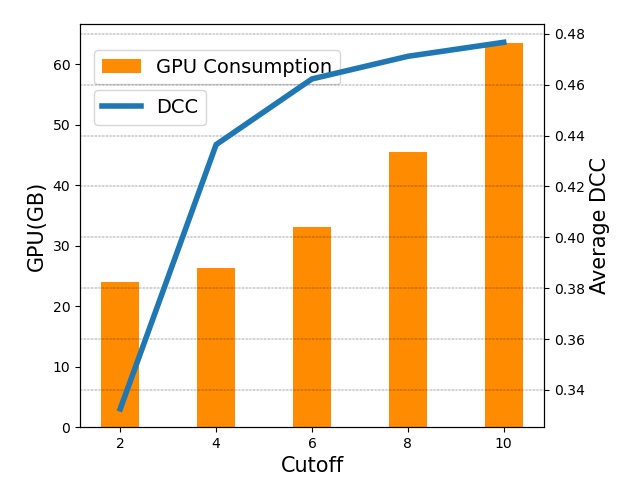
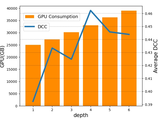
Figure 7. The influence of cutoff $\theta$ and depth for experiment

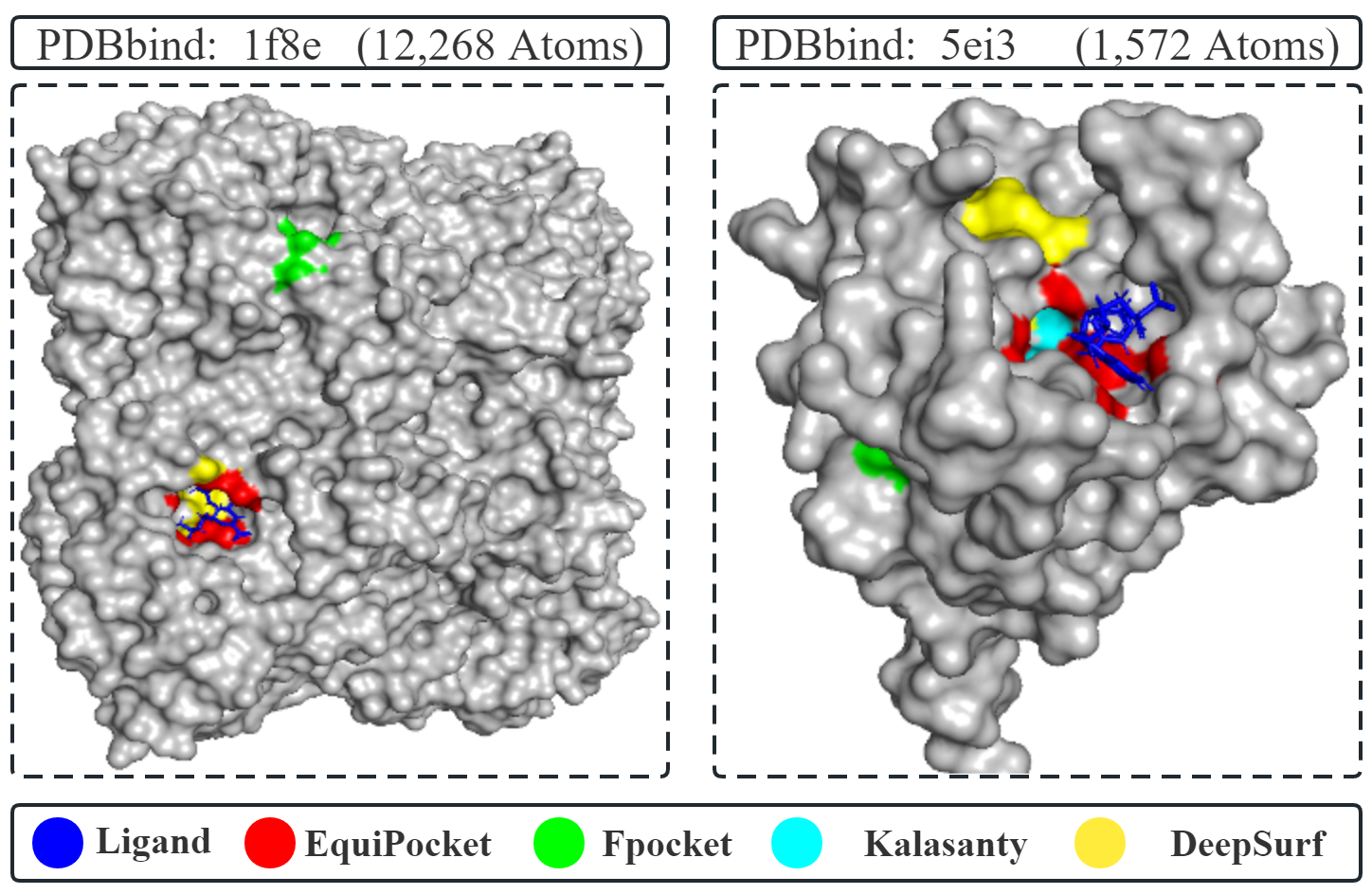
Figure 8. Case Study.

6. Conclusion

In this paper, concentrating on the ligand binding site prediction, we propose a novel E(3)-Equivariant geometric graph framework called EquiPocket, which contains the local geometric modeling module, global structure modeling module, and surface passing module to gather the surface geometric and multi-level structure features in a protein. Experiments demonstrate that our framework is highly generalizable and beneficial, and achieves superior prediction accuracy and computational efficiency compared with the existing methods.

6.1. Future Work

6.1.1. Protein Surface

As demonstrated by our experiments, the geometric information derived from the protein surface plays a significant role in the prediction of binding sites. In this work, we use MSMS (Sanner et al., 1996) to generate the protein surface , which may have an uncertain impact on the prediction results. Therefore, in the future, we will be able to establish a more efficient surface generation method or gather the geometric information of a protein without a fixed protein surface.

6.1.2. Global Structure Model

In this work, we take the existing graph-based models (GAT + EGNN) to gather the multi-level structure information in a protein. However, their capabilities are limited because these models are not entirely tailored to complex structures such as proteins. In the future, we will be able to develop more effective models to gather information from proteins in order to improve the prediction performance of binding sites.

6.1.3. Computing Resources

As the experimental results show, both our EquiPocket and CNN-based methods require a significant amount of computing resources to analyze protein data, which will have a negative impact on their actual deployment. Consequently, when applying our method to real-world problems, it is crucial to consider how to compress algorithm parameters, increase computational efficiency, and decrease resource consumption.

Appendix A Appendix

A.1. The pseudo-code of our EquiPocket framework

0:  Protein structure $\mathcal{G}_{P}$

0:  Candidate Binding sites and their ligandability score

1:  Clean Structure by removing solvent, hydrogens atoms

2:  Create the solvent accessible surface of the protein $\mathbb{S}$ use MSMS

3:  for every $s_{i}$ in $\mathbb{S}$ do

4:     Get its closed protein atom $p_{i}$

5:  end for

6:  Get the surface atom $\mathcal{V}_{S}$ according to the surface points‘s closed protein atom

7:  for every surface atom $i\in\mathcal{V}_{S}$  do

8:     Get their surrounding surface points set $\mathbb{S}_{i}$

9:     Get the geometric embedding ${\bm{g}}_{i}$

10:  end for

11:  Get the global structure embedding ${{\bm{c}}_{i}^{{}^{\prime\prime}}}$ of the protein

12:  for every surface atom $i\in\mathcal{V}_{S}$  do

13:     Get its invariant feature ${\bm{h}}^{(0)}_{i}=[{\bm{c}}^{\prime\prime}_{i},{\bm{g}}_{i}].]$ and equivariant position matrix ${\bm{X}}^{(0)}_{i}=[{\bm{x}}_{i},\bar{{\bm{x}}}_{i}]$

14:     Get the updated embedding ${\bm{h}}_{i}^{(l)}$ and updated coordinates ${\bm{X}}_{i}^{(l)}$ based on our surface-egnn model

15:     Get the dense embedding ${\bm{h}}_{i}$ and position ${\bm{X}}_{i}$ according to its dense attention ${\bm{a}}_{i}$

16:     predict the probability $\hat{{\bm{y}}_{i}}$ as ligandability score and the nearest ligand atom direction ${\bm{d}}_{i}$

17:  end for

18:  Discard protein atoms with probability less than T (T=0.5 in our experiments);

19:  Cluster the remaining protein atoms;

20:  Form binding sites and get the average ligandability score for each cluster;

21:  Rank the predicted binding sites by their ligandability score;

22:  return The candidate binding sites and ligandability score;

Algorithm 1 EquiPocket

A.2. Experiment Details

A.2.1. Cross-validation

We shuffled the training data and divided the data into 5 parts, taking one of them at a time as the validation set. We use 5-fold cross-validation and report the mean and standard deviation.

A.2.2. Parameter Settings

For geometric-based method Fpocket, we use its published tool. For CNN-based methods kalasanty and DeepSurf, we use their published pre-train models. For GNN-based models, the number of layers is set to 3 except GAT. For GAT, we set the number to 1. For GIN, we set the initial $\epsilon$ to 0 and make it trainable. For GCN2, we set the strength of the initial residual connection $\alpha$ to 0.5 and the strength of the identity mapping $\beta$ to 1. For SchNet, EGNN, DimeNet++, SphereNet as baseline models, we set the cutoff distance to 5. For our EquiPocket, we use Adam optimizer for model training with a learning rate of 0.0001 and set the batch size as 8. The basic dimensions of node and edge embeddings are both set to 128. The dropout rate is set to 0.1. The probe radius in MSMS to generate solvent-accessible surface of a protein is set to 1.5.

A.2.3. Baseline Codes

The result of DeepSite comes from (Mylonas et al., 2021), because they did not provide a pre-train model. Table 3 describes sources of baseline codes.

Table 3. Sources of baseline codes and pre-train models.

Methods	URL
fpocker	https://github.com/Discngine/fpocket
kalasanty	https://gitlab.com/cheminfIBB/kalasanty
DeepSurf	https://github.com/stemylonas/DeepSurf
GAT	https://github.com/pyg-team/pytorch_geometric
GCN	https://github.com/pyg-team/pytorch_geometric
GCN2	https://github.com/chennnM/GCNII
SchNet	https://github.com/pyg-team/pytorch_geometric
DimeNet++	https://github.com/pyg-team/pytorch_geometric
EGNN	https://github.com/vgsatorras/egnn/

Table 4. The 5-fold results for EquiPocket.

Methods	Fold	Param	failure	COACH420		HOLO4K		PDBbind2020
		(M)	Rate $\downarrow$	DCC$\uparrow$	DCA$\uparrow$	DCC$\uparrow$	DCA$\uparrow$	DCC$\uparrow$	DCA$\uparrow$
EquiPocket-L	0	0.15	0.598	0.083	0.160	0.038	0.128	0.049	0.124
EquiPocket-L	1	0.15	0.557	0.064	0.165	0.046	0.138	0.055	0.142
EquiPocket-L	2	0.15	0.571	0.074	0.177	0.045	0.139	0.052	0.122
EquiPocket-L	3	0.15	0.462	0.059	0.173	0.042	0.138	0.052	0.129
EquiPocket-L	4	0.15	0.472	0.072	0.180	0.048	0.146	0.049	0.143
EquiPocket-G	0	0.42	0.305	0.135	0.330	0.122	0.400	0.142	0.302
EquiPocket-G	1	0.42	0.291	0.175	0.385	0.128	0.405	0.145	0.302
EquiPocket-G	2	0.42	0.295	0.145	0.357	0.121	0.407	0.145	0.305
EquiPocket-G	3	0.42	0.278	0.169	0.367	0.127	0.406	0.133	0.292
EquiPocket-G	4	0.42	0.292	0.152	0.367	0.133	0.411	0.151	0.308
EquiPocket-LG	0	0.50	0.235	0.225	0.442	0.183	0.498	0.273	0.463
EquiPocket-LG	1	0.50	0.207	0.220	0.460	0.189	0.509	0.280	0.468
EquiPocket-LG	2	0.50	0.203	0.184	0.440	0.180	0.510	0.269	0.459
EquiPocket-LG	3	0.50	0.224	0.215	0.448	0.186	0.500	0.275	0.465
EquiPocket-LG	4	0.50	0.231	0.213	0.431	0.179	0.492	0.272	0.456
EquiPocket	0	1.70	0.054	0.423	0.656	0.341	0.665	0.558	0.715
EquiPocket	1	1.70	0.053	0.431	0.660	0.329	0.668	0.538	0.725
EquiPocket	2	1.70	0.041	0.443	0.664	0.336	0.660	0.550	0.724
EquiPocket	3	1.70	0.051	0.411	0.646	0.338	0.668	0.532	0.723
EquiPocket	4	1.70	0.053	0.407	0.654	0.345	0.652	0.546	0.719

A.2.4. Binding sites center

The CNN-based methods (Jiménez et al., 2017; Aggarwal et al., 2021; Stepniewska-Dziubinska et al., 2020) consider a protein as a 3D image, convert it to a voxel representation by discretizing it into grids and calculate the geometric center of binding site $center_{cnn}$ according to the grid of the cavity or ligand. They label the grid as positive if its geometric center is closer than 4Å to the binding sites geometric center. Therefore, the prediction objects of these models actually contain the grid of ligand atoms. The predicted binding site center $\hat{center_{cnn}}$ of CNN-based methods is calculated according to the positive grid. For our EquiPocket, we label the protein atoms within 4Å of any ligand atom as positive and negative otherwise. Therefore, there is a natural gap in the prediction object between our framework and CNN-based methods, which also lead to the natural gap for the center of predicted binding site. In order to reduce the metric difference caused by the different prediction objects, we get the predicted binding site center $\hat{center}_{equipocket}$ as follow: Ww use $pos_{i}\in\mathbb{R}^{3}$ to represent the position of protein atom $v_{i}$, $center_{i}\in\mathbb{R}^{3}$ to represent the nearest surface point center, $\hat{pos_{i}^{L}}\in\mathbb{R}^{3}$ to represent the predicted position of nearest ligand atom from the protein atom $v_{i}$. The $\hat{pos}_{i}^{L}$ is used to calculate the geometric center of binding site.

(21) $$\widehat{pos}_{i}^{L}=pos_{i}+threshold\cdot\frac{(center_{i}-pos_{i})}{\left|center_{i}-pos_{i}\right|},$$

Where $threshold4$ is set to 4, because we label the protein atoms within 4Å of any ligand atom as positive and negative otherwise.

A.2.5. The 5-fold results for EquiPocket

References

- (1)
- Aggarwal et al. (2021) Rishal Aggarwal, Akash Gupta, Vineeth Chelur, CV Jawahar, and U Deva Priyakumar. 2021. Deeppocket: ligand binding site detection and segmentation using 3d convolutional neural networks. Journal of Chemical Information and Modeling (2021).
- Belgiu and Drăguţ (2016) Mariana Belgiu and Lucian Drăguţ. 2016. Random forest in remote sensing: A review of applications and future directions. ISPRS journal of photogrammetry and remote sensing 114 (2016), 24–31.
- Brylinski and Skolnick (2008) Michal Brylinski and Jeffrey Skolnick. 2008. A threading-based method (FINDSITE) for ligand-binding site prediction and functional annotation. Proceedings of the National Academy of sciences 105, 1 (2008), 129–134.
- Chen et al. (2011) Ke Chen, Marcin J Mizianty, Jianzhao Gao, and Lukasz Kurgan. 2011. A critical comparative assessment of predictions of protein-binding sites for biologically relevant organic compounds. Structure 19, 5 (2011), 613–621.
- Chen et al. (2020) Ming Chen, Zhewei Wei, Zengfeng Huang, Bolin Ding, and Yaliang Li. 2020. Simple and Deep Graph Convolutional Networks. arXiv:2007.02133 [cs.LG]
- Comaniciu and Meer (2002) Dorin Comaniciu and Peter Meer. 2002. Mean shift: A robust approach toward feature space analysis. IEEE Transactions on pattern analysis and machine intelligence 24, 5 (2002), 603–619.
- Da Silva et al. (2018) Franck Da Silva, Jeremy Desaphy, and Didier Rognan. 2018. IChem: a versatile toolkit for detecting, comparing, and predicting protein–ligand interactions. ChemMedChem 13, 6 (2018), 507–510.
- Desaphy et al. (2015) Jérémy Desaphy, Guillaume Bret, Didier Rognan, and Esther Kellenberger. 2015. sc-PDB: a 3D-database of ligandable binding sites—10 years on. Nucleic acids research 43, D1 (2015), D399–D404.
- Dias et al. (2017) Sérgio ED Dias, Quoc T Nguyen, Joaquim A Jorge, and Abel JP Gomes. 2017. Multi-GPU-based detection of protein cavities using critical points. Future Generation Computer Systems 67 (2017), 430–440.
- Faller et al. (2015) Christina E Faller, E Prabhu Raman, Alexander D MacKerell, and Olgun Guvench. 2015. Site Identification by Ligand Competitive Saturation (SILCS) simulations for fragment-based drug design. In Fragment-Based Methods in Drug Discovery. Springer, 75–87.
- Gonczarek et al. (2016) A. Gonczarek, J. M. Tomczak, S Zaręba, J. Kaczmar, P Dąbrowski, and M. J. Walczak. 2016. Learning Deep Architectures for Interaction Prediction in Structure-based Virtual Screening. (2016).
- Han et al. (2022) J. Han, Y. Rong, T. Xu, and W. Huang. 2022. Geometrically Equivariant Graph Neural Networks: A Survey. (2022).
- Hendlich et al. (1997) Manfred Hendlich, Friedrich Rippmann, and Gerhard Barnickel. 1997. LIGSITE: automatic and efficient detection of potential small molecule-binding sites in proteins. Journal of Molecular Graphics and Modelling 15, 6 (1997), 359–363.
- Huang et al. (2022) W. Huang, J. Han, Y. Rong, T. Xu, F. Sun, and J. Huang. 2022. Equivariant Graph Mechanics Networks with Constraints. arXiv e-prints (2022).
- Huang et al. (2020) W. Huang, Y. Rong, T. Xu, F. Sun, and J. Huang. 2020. Tackling Over-Smoothing for General Graph Convolutional Networks. (2020).
- Jiang et al. (2019) Mingjian Jiang, Zhiqiang Wei, Shugang Zhang, Shuang Wang, Xiaofeng Wang, and Zhen Li. 2019. Frsite: protein drug binding site prediction based on faster R–CNN. Journal of Molecular Graphics and Modelling 93 (2019), 107454.
- Jiménez et al. (2017) José Jiménez, Stefan Doerr, Gerard Martínez-Rosell, Alexander S Rose, and Gianni De Fabritiis. 2017. DeepSite: protein-binding site predictor using 3D-convolutional neural networks. Bioinformatics 33, 19 (2017), 3036–3042.
- Kandel et al. (2021) Jeevan Kandel, Hilal Tayara, and Kil To Chong. 2021. PUResNet: prediction of protein-ligand binding sites using deep residual neural network. Journal of cheminformatics 13, 1 (2021), 1–14.
- Kip and Welling (2016) T. N. Kip and M. Welling. 2016. Semi-Supervised Classification with Graph Convolutional Networks. (2016).
- Kipf and Welling (2016) Thomas N Kipf and Max Welling. 2016. Semi-supervised classification with graph convolutional networks. arXiv preprint arXiv:1609.02907 (2016).
- Klicpera et al. (2020a) J. Klicpera, S. Giri, J. T. Margraf, and S Günnemann. 2020a. Fast and Uncertainty-Aware Directional Message Passing for Non-Equilibrium Molecules. (2020).
- Klicpera et al. (2020b) J. Klicpera, J. Gro, and S Günnemann. 2020b. Directional Message Passing for Molecular Graphs. (2020).
- Krivák and Hoksza (2015) Radoslav Krivák and David Hoksza. 2015. Improving protein-ligand binding site prediction accuracy by classification of inner pocket points using local features. Journal of cheminformatics 7, 1 (2015), 1–13.
- Krivák and Hoksza (2018) Radoslav Krivák and David Hoksza. 2018. P2Rank: machine learning based tool for rapid and accurate prediction of ligand binding sites from protein structure. Journal of cheminformatics 10, 1 (2018), 1–12.
- Laskowski (1995) Roman A Laskowski. 1995. SURFNET: a program for visualizing molecular surfaces, cavities, and intermolecular interactions. Journal of molecular graphics 13, 5 (1995), 323–330.
- Laurie and Jackson (2005) Alasdair TR Laurie and Richard M Jackson. 2005. Q-SiteFinder: an energy-based method for the prediction of protein–ligand binding sites. Bioinformatics 21, 9 (2005), 1908–1916.
- Le Guilloux et al. (2009) Vincent Le Guilloux, Peter Schmidtke, and Pierre Tuffery. 2009. Fpocket: an open source platform for ligand pocket detection. BMC bioinformatics 10, 1 (2009), 1–11.
- Levitt and Banaszak (1992) David G Levitt and Leonard J Banaszak. 1992. POCKET: a computer graphies method for identifying and displaying protein cavities and their surrounding amino acids. Journal of molecular graphics 10, 4 (1992), 229–234.
- Liu et al. (2021) Yi Liu, Limei Wang, Meng Liu, Xuan Zhang, Bora Oztekin, and Shuiwang Ji. 2021. Spherical Message Passing for 3D Graph Networks. arXiv:2102.05013 [cs.LG]
- Macari et al. (2019) Gabriele Macari, Daniele Toti, and Fabio Polticelli. 2019. Computational methods and tools for binding site recognition between proteins and small molecules: from classical geometrical approaches to modern machine learning strategies. Journal of computer-aided molecular design 33, 10 (2019), 887–903.
- Mylonas et al. (2021) Stelios K Mylonas, Apostolos Axenopoulos, and Petros Daras. 2021. DeepSurf: a surface-based deep learning approach for the prediction of ligand binding sites on proteins. Bioinformatics 37, 12 (2021), 1681–1690.
- Ngan et al. (2012) Chi-Ho Ngan, David R Hall, Brandon Zerbe, Laurie E Grove, Dima Kozakov, and Sandor Vajda. 2012. FTSite: high accuracy detection of ligand binding sites on unbound protein structures. Bioinformatics 28, 2 (2012), 286–287.
- Ragoza et al. (2017) Matthew Ragoza, Joshua Hochuli, Elisa Idrobo, Jocelyn Sunseri, and David Ryan Koes. 2017. Protein–ligand scoring with convolutional neural networks. Journal of chemical information and modeling 57, 4 (2017), 942–957.
- Rang (2006) HP Rang. 2006. The receptor concept: pharmacology’s big idea. British journal of pharmacology 147, S1 (2006), S9–S16.
- Richmond (1984) Timothy J Richmond. 1984. Solvent accessible surface area and excluded volume in proteins: Analytical equations for overlapping spheres and implications for the hydrophobic effect. Journal of molecular biology 178, 1 (1984), 63–89.
- Sabrina et al. (2018) Sabrina, Jaeger, Simone, Fulle, Samo, and Turk. 2018. Mol2vec: Unsupervised Machine Learning Approach with Chemical Intuition. Journal of Chemical Information & Modeling (2018).
- Sanner et al. (1996) M. F. Sanner, A. J. Olson, and J. C. Spehner. 1996. Reduced SURFACE: An efficient way to compute molecular surfaces. Peptide Science 38, 3 (1996), 305–320.
- Satorras et al. (2021a) Vıctor Garcia Satorras, Emiel Hoogeboom, and Max Welling. 2021a. E (n) equivariant graph neural networks. In International conference on machine learning. PMLR, 9323–9332.
- Satorras et al. (2021b) V. G. Satorras, E. Hoogeboom, and M. Welling. 2021b. E(n) Equivariant Graph Neural Networks. (2021).
- Schütt et al. (2017) Kristof T. Schütt, Pieter Jan Kindermans, Huziel E. Sauceda, Stefan Chmiela, Alexandre Tkatchenko, and Klaus-Robert Müller. 2017. SchNet: A continuous-filter convolutional neural network for modeling quantum interactions. In Advances in Neural Information Processing Systems.
- Stepniewska-Dziubinska et al. (2020) Marta M Stepniewska-Dziubinska, Piotr Zielenkiewicz, and Pawel Siedlecki. 2020. Improving detection of protein-ligand binding sites with 3D segmentation. Scientific reports 10, 1 (2020), 1–9.
- Sun et al. (2019) M. Sun, S. Zhao, G. Coryandar, E. Olivier, J. Zhou, and F. Wang. 2019. Graph convolutional networks for computational drug development and discovery. Briefings in Bioinformatics (2019).
- Tosco et al. (2014) Paolo Tosco, Nikolaus Stiefl, and Gregory Landrum. 2014. Bringing the MMFF force field to the RDKit: implementation and validation. Journal of Cheminformatics,6,1(2014-07-12) 6, 1 (2014), 37.
- Toti et al. (2018) Daniele Toti, Le Viet Hung, Valentina Tortosa, Valentina Brandi, and Fabio Polticelli. 2018. LIBRA-WA: a web application for ligand binding site detection and protein function recognition. Bioinformatics 34, 5 (2018), 878–880.
- Velikovi et al. (2017) Petar Velikovi, G. Cucurull, A. Casanova, A. Romero, P Lió, and Y. Bengio. 2017. Graph Attention Networks. (2017).
- Wang et al. (2004) Renxiao Wang, Xueliang Fang, Yipin Lu, and Shaomeng Wang. 2004. The PDBbind database: collection of binding affinities for protein-ligand complexes with known three-dimensional structures. Journal of Medicinal Chemistry 47, 12 (2004), 2977–80.
- Wang et al. (2000) Renxiao Wang, Ying Gao, and Luhua Lai. 2000. LigBuilder: a multi-purpose program for structure-based drug design. Molecular modeling annual 6 (2000), 498–516.
- Weisel et al. (2007) Martin Weisel, Ewgenij Proschak, and Gisbert Schneider. 2007. PocketPicker: analysis of ligand binding-sites with shape descriptors. Chemistry Central Journal 1, 1 (2007), 1–17.
- Xu et al. (2018) K. Xu, W. Hu, J. Leskovec, and S. Jegelka. 2018. How Powerful are Graph Neural Networks? (2018).
- Zhang et al. (2022) Yang Zhang, Gengmo Zhou, Zhewei Wei, and Hongteng Xu. 2022. Predicting Protein-Ligand Binding Affinity via Joint Global-Local Interaction Modeling. arXiv preprint arXiv:2209.13014 (2022).