Streaming probabilistic tensor train decomposition

Abstract

The Bayesian streaming tensor decomposition method is a novel method to discover the low-rank approximation of streaming data. However, when the streaming data comes from a high-order tensor, tensor structures of existing Bayesian streaming tensor decomposition algorithms may not be suitable in terms of representation and computation power. In this paper, we present a new Bayesian streaming tensor decomposition method based on tensor train (TT) decomposition. Especially, TT decomposition renders an efficient approach to represent high-order tensors. By exploiting the streaming variational inference (SVI) framework and TT decomposition, we can estimate the latent structure of high-order incomplete noisy streaming tensors. The experiments in synthetic and real-world data show the accuracy of our algorithm compared to the state-of-the-art Bayesian streaming tensor decomposition approaches.

1 Introduction

Multiway data or multidimensional arrays, represented by tensors, are ubiquitous in real-world applications, such as recommendation systems [1, 2], computer version [3], medical imaging [4] and uncertainty quantification [5]. How to process, analyze and utilize such high-volume tensor data is a fundamental problem in machine learning [6, 7], data mining [8] and signal processing [9].

Effective numerical techniques, such as CANDECOMP/PARAFAC (CP) decomposition [10, 11, 12] and Tucker decomposition [13, 14] are the most commonly used tensor decomposition approaches and have been proposed to compress full tensors and to obtain their low-rank representations. CP decomposition approximates a tensor by a sum of rank-one tensors, while Tucker decomposition decomposes a tensor into a core tensor and several factor matrices. Since CP decomposition can be seen as a special case of Tucker decomposition [15], Tucker decomposition is more flexible than CP decomposition. However, due to the existence of a core tensor, Tucker decomposition also brings challenges in both modeling and computation. In this paper, we mainly focus on Tensor Train (TT) decomposition [16], which combines the advantages of CP and Tucker decomposition, because it provides a space-saving model called TT format while preserving the representation power.

This paper is interested in the decomposition of streaming data. Due to the stress on database capacity and privacy, streaming data is generated continuously by different of data sources and in small sizes, such as log files from web application [17] and information from social networks [18]. Recently, several works decompose fast streaming data, e.g. POST [19] and BASS-Tucker [20]. POST and BASS-Tucker are probabilistic streaming tensor decomposition algorithm based on Bayesian formulation of CP decomposition and Tucker decomposition respectively. Although both of POST and BASS-Tucker are powerful streaming decomposition approach and can adapt to a large amount of applications, the latent factors (CP factors) in POST are lack of representation power and BASS-Tucker is ambitious to execute and comprehensive due to the complex reducing model and high time complexity.

To address these challenges, we develop SPTT, a Streaming Probabilistic TT decomposition approach. The main contributions of this work are three-folds: First, we propose a Bayesian tensor decomposition method based on TT decomposition, which can be adopted to analysis high-order incomplete noisy streaming data; Second, motivated by the Bayesian TT representation for batch-mode data in [21], we introduce a probabilistic TT model and exploit the streaming variational inference (SVI) method on it for streaming data analysis; Third, both synthetic and real-world data are used in demonstrating the accuracy of our algorithm.

The paper is organized as follows. We review the tensor basics and tensor train decomposition in section 2, and in 3 we present our SPTT algorithm with streaming variational inference. In section 4, we demonstrate the accuracy of our algorithm in both synthetic and real-worlds dataset. Finally, in section section 5, we make some conclusions.

2 Background

2.1 Tensor basics and notation

In this paper, we denote scalar, vector, matrix and tensor variables, respectively, by lowercase letters (e.g. $x$), boldface lowercase letters (e.g. $\mathbf{x}$), boldface capital letters (e.g. $\mathbf{X}$), and boldface Euler script letters (e.g. $\boldsymbol{\mathscr{X}}$). For a $D$-th order tensor $\boldsymbol{\mathscr{X}}\in\mathbb{R}^{N_{1}\times\cdots\times N_{D}}$, we denote the $\mathbf{j}:=(j_{1},\cdots,j_{D})$-th element of $\boldsymbol{\mathscr{X}}$ by $x_{\mathbf{j}}$, where $j_{d}=1,\ldots,N_{d}$ for $d=1,\ldots,D$.

2.2 Tensor train decomposition

Given TT-ranks $r_{k}$ in vector $\mathbf{r}=(r_{1},\ldots,r_{D})$ with $r_{1}=r_{D}=1$, each element of a $D$-th order tensor $\boldsymbol{\mathscr{X}}$ is tensorized by TT decomposition

$$x_{\mathbf{j}}\approx a_{\mathbf{j}}=\prod_{d=1}^{D}\boldsymbol{\mathscr{G}}^{(d)}_{j_{d}},\quad\boldsymbol{\mathscr{X}}\approx\boldsymbol{\mathscr{A}}=\langle\langle\boldsymbol{\mathscr{G}}^{(1)},\ldots,\boldsymbol{\mathscr{G}}^{(D)}\rangle\rangle$$ (1)

where $\boldsymbol{\mathscr{G}}^{(d)}_{j_{d}}\in\mathbb{R}^{r_{d-1}\times r_{d}}$ is the $j_{d}$-th slice of TT-cores $\boldsymbol{\mathscr{G}}^{(d)}\in\mathbb{R}^{r_{d-1}\times N_{d}\times r_{d}}$, for $j_{d}=1,\ldots,N_{d}$, $d=1,\ldots,D$, and $a_{\mathbf{j}}$ is the $\mathbf{j}$-th element of tensor $\boldsymbol{\mathscr{A}}$ and approximates $x_{\mathbf{j}}$. In other words, TT decomposition is to decompose a $D$-th order tensor $\boldsymbol{\mathscr{X}}$ into a sequence of three-way factor tensors, collected by a TT-format tensor $\boldsymbol{\mathscr{A}}$. Figure 1 illustrate the TT decomposition.

Figure 1: TT decomposition for an element (TT-format)

To find the optimal TT-cores under partial observations, TT decomposition minimizes a mean square loss,

$$\mathcal{L}(\boldsymbol{\mathscr{A}})=\|\boldsymbol{\mathscr{X}}_{\Omega}-\boldsymbol{\mathscr{A}}_{\Omega}\|_{F}^{2}$$ (2)

where $\boldsymbol{\mathscr{X}}_{\Omega}$ and $\boldsymbol{\mathscr{A}}_{\Omega}$ are vectors containing $x_{\mathbf{j}}$ and $a_{\mathbf{j}}$, respectively, $\mathbf{j}\in\Omega$. Here $\Omega$ is the index set of observed tensor entries. We can use alternating least squares [22] to update each TT core alternatively, given all the other fixed. In addition, gradient-based approaches [23] can also be used to minimize the loss function.

Instead of explicitly storing the original tensor, one can choose to maintain and use the TT-cores because of the convenience and effectiveness of TT-cores. Assuming that $r_{d}=R,\,d=2,\dots.D-1$, and that $N_{d}=N,\,d=1,\dots,D$, the storage of the tensor $\boldsymbol{\mathscr{X}}$ in the standard form is $O(N^{D})$, while the storage in TT-format $\boldsymbol{\mathscr{A}}$ is $O(NDR^{2})$, which is linear to the tensor order. Consider two tensors $\boldsymbol{\mathscr{X}},\boldsymbol{\mathscr{Y}}\in\mathbb{R}^{N_{1}\times\cdots\times N_{D}}$, the inner product is defined as

$$\langle\boldsymbol{\mathscr{X}},\boldsymbol{\mathscr{Y}}\rangle:=\sum_{\mathbf{j}}x_{\mathbf{j}}y_{\mathbf{j}}.$$ (3)

Similarly, using the TT-format of $\boldsymbol{\mathscr{X}},\boldsymbol{\mathscr{Y}}$, one can implement the inner product with $O(DNR^{3})$ operations rather than $O(N^{D})$ (Cf. Algorithm 4 in [16]). Using the inner product, the Frobenius norm $\|\boldsymbol{\mathscr{X}}\|_{F}=\sqrt{\langle\boldsymbol{\mathscr{X}},\boldsymbol{\mathscr{X}}\rangle}$ and the distance between two tensors $\|\boldsymbol{\mathscr{X}}-\boldsymbol{\mathscr{Y}}\|_{F}$ can be efficiently calculated. Besides, when TT-ranks are small enough, the TT-format is also efficient for other basic linear algebra operations, such as matrix-by-vector products, scalar multiplications, see [16] for details.

3 Bayesian model for streaming tensor train decomposition

In this section, we first develop the probabilistic model of TT decomposition, where the Gaussian noise is included. After that, streaming data is introduced and a posterior inference for TT-cores is developed by streaming variational inference (SVI) [24]. Finally, we present the streaming probabilistic tensor train decomposition (SPTT) algorithm.

3.1 Probabilistic modeling of tensor train decomposition

The standard TT decomposition, like [22, 23], use the point estimation to approximate the TT-cores and is not capable of evaluating the uncertainty, which can vary among each slice in a TT core. To overcome this problem, inspired by a Bayesian TT representation for batch-mode data in [21], we introduce a Bayesian TT model for streaming data.

We first specify $\{\boldsymbol{\mathscr{G}}^{(d)}\}_{d=1}^{D}$ from a Gaussian prior,

$$p(\{\boldsymbol{\mathscr{G}}^{(d)}\}_{d=1}^{D})=\prod_{d=1}^{D}\prod_{k=1}^{r_{d-1}}\prod_{l=1}^{r_{d}}\mathcal{N}\left(\boldsymbol{\mathscr{G}}^{(d)}_{k,:,l}\bigg{|}\mathbf{m}_{\boldsymbol{\mathscr{G}}_{k,:,l}^{(d)}},v\mathbf{I}\right),$$ (4)

which indicates that each fiber $\boldsymbol{\mathscr{G}}^{(d)}_{k,:,l}$ admits a Gaussian distribution with mean $\mathbf{m}_{\boldsymbol{\mathscr{G}}_{k,:,l}}^{(d)}$, and covariance matrix $v\mathbf{I}$. $v$ is a scalar and controls the flatness of the Gaussian prior.

Given the TT-cores $\{\boldsymbol{\mathscr{G}}^{(d)}\}_{d=1}^{D}$, the likelihood of an observed entry value $x_{\mathbf{j}}$ is

$$p(x_{\mathbf{j}}|\{\boldsymbol{\mathscr{G}}^{(d)}\}_{d=1}^{D},\tau)=\mathcal{N}\left(x_{\mathbf{j}}\big{|}\prod_{d=1}^{D}\boldsymbol{\mathscr{G}}^{(d)}_{j_{d}},\tau^{-1}\right),$$ (5)

where $\tau$ is the inverse of the noise variance. Since the Gamma distribution, because of its non-negative and long tail, provides a good model for $\tau$, we assign a Gamma prior over $\tau$

$$p(\tau|\alpha_{0},\beta_{0})=\operatorname{Gam}(\tau|\alpha_{0},\beta_{0}).$$ (6)

where $\alpha_{0}$ and $\beta_{0}$ are hyperparameters of the Gamma distribution. The density function of a Gamma distribution is

$$p(x|\alpha,\beta)=\frac{x^{\alpha-1}e^{-\beta x}\beta^{\alpha}}{\Gamma(\alpha)},$$

where $\Gamma(\alpha)$ is a Gamma function.

The joint probability is then given by combining (4) with (5)-(6),

$$p\left(x_{\mathbf{j}\in\Omega},\{\boldsymbol{\mathscr{G}}^{(d)}\}_{d=1}^{D},\tau\right) =\operatorname{Gam}(\tau|\alpha_{0},\beta_{0})$$ (7)

$$\cdot\prod_{d=1}^{D}\prod_{k=1}^{r_{d-1}}\prod_{l=1}^{r_{d}}\left(\boldsymbol{\mathscr{G}}^{(d)}_{k,:,l}\bigg{|}\mathbf{m}_{\boldsymbol{\mathscr{G}}_{k,:,l}^{(d)}},v\mathbf{I}\right)$$

$$\cdot\prod_{\mathbf{j}\in\Omega}\mathcal{N}\left(x_{\mathbf{j}}\big{|}\prod_{d=1}^{D}\boldsymbol{\mathscr{G}}^{(d)}_{j_{d}},\tau^{-1}\right).$$

3.2 Bayesian streaming inference

We introduce SPTT, our posterior inference algorithm for streaming data, based on TT decomposition in subsection 3.1 and the streaming variational inference (SVI) [24]. Assume that the observed tensor entries are provided in a series of batches, $\{B_{1},B_{2},\ldots\}$, we aim to conduct the posterior inference for TT-cores $\{\boldsymbol{\mathscr{G}}^{(d)}\}_{d=1}^{D}$ and the inverse of noise variance $\tau$ upon receiving each data batch $B_{t}$, without revisiting the previous batches $\tilde{B}=\{B_{1},\ldots,B_{t-1}\}$.

Assume the prior distribution of $\mathbf{\theta}=\{\{\boldsymbol{\mathscr{G}}^{(d)}\}_{d=1}^{D},\tau\}$ is $p(\mathbf{\theta})$. Denote $\Omega_{t}$ is the index set of $t$-th data batch $B_{t}$. For the first data batch $B_{1}=\{x_{\mathbf{j}}\}_{\mathbf{j}\in\Omega_{1}}$, the posterior $p(\mathbf{\theta}|B_{1})$ can be calculated via Bayes’ rule:

$$p(\mathbf{\theta}|B_{1})\propto p(\mathbf{\theta})p(B_{1}|\mathbf{\theta}),$$ (8)

where $p(B_{1}|\mathbf{\theta})=\prod_{\mathbf{j}\in\Omega_{1}}p(x_{\mathbf{j}}|\mathbf{\theta})$. Similarly, when receiving the newly data batch $B_{t}=\{x_{\mathbf{j}}\}_{\mathbf{j}\in\Omega_{t}}$, the incremental posterior is given by

$$p(\mathbf{\theta}|\tilde{B}\cup B_{t})\propto p(\mathbf{\theta}|\tilde{B})p(B_{t}|\mathbf{\theta}),$$ (9)

The proportional relationship in (9) motivates us to adopt a recursive process of streaming inference for $\mathbf{\theta}$. However, the multilinear product of TT-cores $\{\boldsymbol{\mathscr{G}}^{(d)}\}_{d=1}^{D}$ in (5) results in the posterior update intractable. To overcome the problem, we introduce a factorized variational posterior distribution $q_{t-1}(\mathbf{\theta})=\prod_{i}q_{t-1}(\mathbf{\theta}_{i})$ to approximate $p(\mathbf{\theta}|\tilde{B})$. With receiving new data batch $B_{t}$, we can obtain a new distribution $\tilde{q}_{t}(\mathbf{\theta})=q_{t-1}(\mathbf{\theta})p(B_{t}|\mathbf{\theta})$, which is proportional to $p(\mathbf{\theta},\tilde{B}\cup B_{t})$. We approximate posterior $p(\mathbf{\theta}|\tilde{B}\cup B_{t})$ with $q_{t}(\mathbf{\theta})$,

$$q_{t}(\mathbf{\theta})=q_{t}(\{\boldsymbol{\mathscr{G}}^{(d)}\}_{d=1}^{D},\tau)=q_{t}(\tau)\prod_{d=1}^{D}\prod_{k=1}^{r_{d-1}}\prod_{l=1}^{r_{d}}\prod_{j_{d}}^{N_{d}}q_{t}\left(\boldsymbol{\mathscr{G}}^{(d)}_{k,j_{d},l}\right).$$ (10)

based on the only assumption that each entries in the TT-cores and the inverse of noise variance are independent. To be noticed, $q_{t}(\theta)$ is also in a factorized form as $q_{t-1}(\mathbf{\theta})$, and can be initialized with $q_{0}(\mathbf{\theta})=p(\mathbf{\theta})$. From the variational inference framework [25], we minimize the Kullback-Leibler (KL) divergence between $\frac{1}{C}\tilde{q}_{t}(\mathbf{\theta})$ and $q_{t}(\mathbf{\theta})$, i.e. $\operatorname{KL}(\frac{1}{C}\tilde{q}_{t}(\mathbf{\theta}||q_{t}(\mathbf{\theta}))$, where $C$ is a normalization constant. This is equivalent to maximize a variational model evidence lower bound (ELBO) [25],

$$\mathcal{L}(q_{t}(\mathbf{\theta}))=\mathbb{E}_{q_{t}}\left[\log\left(\frac{q_{t-1}(\mathbf{\theta})p(B_{t}|\mathbf{\theta})}{q_{t}(\mathbf{\theta})}\right)\right].$$ (11)

Due to the factorized form (10), the particular functional forms of the individual factors $q_{t}(\mathbf{\theta}_{i})$ can be explicitly derived in turn. The update rule for the $i$-th factor based on the maximization of $\mathcal{L}(q_{t}(\mathbf{\theta}))$ is then given by

$$\log q_{t}(\mathbf{\theta}_{i})=\mathbb{E}_{q_{t}(\theta\setminus\mathbf{\theta}_{i})}\left[\log q_{t-1}(\mathbf{\theta})p(B_{t}|\mathbf{\theta})\right]+\operatorname{const},$$ (12)

where $\mathbb{E}_{q_{t}(\theta\setminus\mathbf{\theta}_{i})}$ denotes an expectation w.r.t the $q_{t}$ distributions over all variables except $\mathbf{\theta}_{i}$.

3.2.1 Posterior distribution of TT-cores

Upon the factorized form (10), the inference of an element of TT-cores $\boldsymbol{\mathscr{G}}_{k,j_{d},l}^{(d)}$ can be performed by receiving the messages from the $t$-th data batch $B_{t}$ and the updated information of the whole TT-cores, where $k=1,\ldots,r_{d-1}$, $l=1,\ldots r_{d}$, $j_{d}=1,\ldots,N_{d}$. By applying (12), the optimized form of $\boldsymbol{\mathscr{G}}_{k,j_{d},l}^{(d)}$ is given as follows,

$$\log q_{t}(\boldsymbol{\mathscr{G}}_{k,j_{d},l}^{(d)})=\mathbb{E}_{q_{t}(\mathbf{\theta}\setminus\boldsymbol{\mathscr{G}}_{k,j_{d},l}^{(d)})}\left[\log q_{t-1}\left(\theta\right)p(B_{t}|\theta)\right]+\operatorname{const}.$$ (13)

Obviously, the approximation posterior keeps the same form as the updated one, i.e., Gaussian distribution,

$$q_{t}(\boldsymbol{\mathscr{G}}_{k,j_{d},l}^{(d)})=\mathcal{N}(\boldsymbol{\mathscr{G}}_{k,j_{d},l}^{(d)}|\hat{m}_{\boldsymbol{\mathscr{G}}_{k,j_{d},l}^{(d)}},\hat{v}_{\boldsymbol{\mathscr{G}}_{k,j_{d},l}^{(d)}}).$$ (14)

The variance and mean, derived from derivation (13) w.r.t $\boldsymbol{\mathscr{G}}_{k,j_{d},l}^{(d)}$, can be updated by

$$\hat{v}_{\boldsymbol{\mathscr{G}}_{k,j_{d},l}^{(d)}}=\left({v}_{\boldsymbol{\mathscr{G}}_{k,j_{d},l}^{(d)}}^{-1}+\tau\sum_{\mathbf{j}\in\Omega_{t}^{j_{d}}}\mathbb{E}\left[b^{(<d)^{T}}_{(k-1)r_{d-1}+k}\right]\mathbb{E}\left[b^{(>d)}_{(l-1)r_{d}+l}\right]\right)^{-1},$$ (15)

$$\hat{m}_{\boldsymbol{\mathscr{G}}_{k,j_{d},l}^{(d)}} =\hat{v}_{\boldsymbol{\mathscr{G}}_{k,j_{d},l}^{(d)}}\left(\frac{m_{\boldsymbol{\mathscr{G}}_{k,j_{d},l}^{(d)}}}{v_{\boldsymbol{\mathscr{G}}_{k,j_{d},l}^{(d)}}}+\tau\sum_{\mathbf{j}\in\Omega_{t}^{j_{d}}}\left(x_{\mathbf{j}}\mathbb{E}\left[e^{(<d)^{T}}_{k}\right]\mathbb{E}\left[e^{(>d)}_{l}\right]-\right.\right.$$ (16)

$$\left.\left.\sum_{k^{\prime}=1,k^{\prime}\neq k}^{r_{d-1}}\sum_{l^{\prime}=1,l^{\prime}\neq l}^{r_{d}}\mathbb{E}\left[b^{(<d)^{T}}_{(k-1)r_{d-1}+k^{\prime}}\right]m_{\boldsymbol{\mathscr{G}}^{(d)}_{k^{\prime},j_{d},l^{\prime}}}\mathbb{E}\left[b^{(>d)}_{(l-1)r_{d}+l^{\prime}}\right]\right)\right),$$

with

$$\mathbb{E}\left[e^{(<d)^{T}}_{k}\right]=\prod_{i=1}^{d-1}\mathbb{E}\left[\boldsymbol{\mathscr{G}}^{(i)}_{j_{i}}\right],\quad\mathbb{E}\left[e^{(>d)}_{k}\right]=\prod_{i=d}^{D}\mathbb{E}\left[\boldsymbol{\mathscr{G}}^{(i)}_{j_{i}}\right],$$ (17)

$$\mathbb{E}\left[b^{(<d)^{T}}\right]=\prod_{i=1}^{d-1}\mathbb{E}\left[\boldsymbol{\mathscr{G}}^{(i)}_{j_{i}}\otimes\boldsymbol{\mathscr{G}}^{(i)}_{j_{i}}\right],\quad\mathbb{E}\left[b^{(>d)}\right]=\prod_{i=d+1}^{D}\mathbb{E}\left[\boldsymbol{\mathscr{G}}^{(i)}_{j_{i}}\otimes\boldsymbol{\mathscr{G}}^{(i)}_{j_{i}}\right].$$ (18)

where $\hat{v}_{\boldsymbol{\mathscr{G}}_{k,j_{d},l}^{(d)}}$ and $\hat{m}_{\boldsymbol{\mathscr{G}}_{k,j_{d},l}^{(d)}}$ are the variance and mean of the element $\boldsymbol{\mathscr{G}}_{k,j_{d},l}^{(d)}$ after the $t$-th data batch, while ${v}_{\boldsymbol{\mathscr{G}}_{k,j_{d},l}^{(d)}}$ and ${m}_{\boldsymbol{\mathscr{G}}_{k,j_{d},l}^{(d)}}$ are the updated variance and mean after the $(t-1)$-th data batch. The subscript $\Omega_{t}^{j_{d}}$ represents the indexes of $t$-th batch data with $d$-th index fixing as $j_{d}$. The expression $\mathbb{E}[\cdot]$ denotes the expectation with respect to all random variables involved. From (17) and (18), we can see that, for $d=1,\ldots,D$, $e^{(<d)^{T}}$ and $b^{(<d)^{T}}$ are row vectors, while $e^{(>d)}$ and $b^{(>d)}$ are column vectors. The subscript of them denotes an element in a vector, e.g. $e^{(<d)^{T}}_{k}$ is the $k$-th element in vector $e^{(<d)^{T}}$. To compute $\mathbb{E}\left[\boldsymbol{\mathscr{G}}^{(i)}_{j_{i}}\otimes\boldsymbol{\mathscr{G}}^{(i)}_{j_{i}}\right]$ in (18), we introduce the following lemma.

Lemma 1.

The expectation of Kronecker product $\boldsymbol{\mathscr{G}}^{(i)}_{j_{i}}\otimes\boldsymbol{\mathscr{G}}^{(i)}_{j_{i}}$ in (18) can be calculated by

$$\mathbb{E}\left[\boldsymbol{\mathscr{G}}^{(i)}_{j_{i}}\otimes\boldsymbol{\mathscr{G}}^{(i)}_{j_{i}}\right]=\mathbb{E}\left[\boldsymbol{\mathscr{G}}^{(i)}_{j_{i}}\right]\otimes\mathbb{E}\left[\boldsymbol{\mathscr{G}}^{(i)}_{j_{i}}\right]+\mathbb{E}\left[\left(\boldsymbol{\mathscr{G}}^{(i)}_{j_{i}}-\mathbb{E}\left[\boldsymbol{\mathscr{G}}^{(i)}_{j_{i}}\right]\right)\otimes\left(\boldsymbol{\mathscr{G}}^{(i)}_{j_{i}}-\mathbb{E}\left[\boldsymbol{\mathscr{G}}^{(i)}_{j_{i}}\right]\right)\right],$$

and its element-wise form is

$$\mathbb{E}\left[\boldsymbol{\mathscr{G}}^{(i)}_{k,j_{i},l}\boldsymbol{\mathscr{G}}^{(i)}_{k^{\prime},j_{i},l^{\prime}}\right]=\mathbb{E}\left[\boldsymbol{\mathscr{G}}^{(i)}_{k,j_{i},l}\right]\mathbb{E}\left[\boldsymbol{\mathscr{G}}^{(i)}_{k^{\prime},j_{i},l^{\prime}}\right]+v_{\boldsymbol{\mathscr{G}}_{k,j_{i},l}^{(i)}}\delta\left(k-k^{\prime}\right)\delta\left(l-l^{\prime}\right).$$

Proof.

From equation (10), we can see any two entries in $\boldsymbol{\mathscr{G}}^{(i)}_{j_{i}}$ are independent,

$$\mathbb{E}\left[\boldsymbol{\mathscr{G}}^{(i)}_{k,j_{i},l}\boldsymbol{\mathscr{G}}^{(i)}_{k^{\prime},j_{i},l^{\prime}}\right]=\mathbb{E}\left[\boldsymbol{\mathscr{G}}^{(i)}_{k,j_{i},l}\right]\mathbb{E}\left[\boldsymbol{\mathscr{G}}^{(i)}_{k^{\prime},j_{i},l^{\prime}}\right]+v_{\boldsymbol{\mathscr{G}}_{k,j_{i},l}^{(i)}}\delta\left(k-k^{\prime}\right)\delta\left(l-l^{\prime}\right),$$

where $\delta(x)=1$ if $x=0$ and zero otherwise. Let $p=r_{i-1}(k-1)+l,\ q=r_{i}(k^{\prime}-1)+l^{\prime}$, then

$$\mathbb{E}\left[\boldsymbol{\mathscr{G}}^{(i)}_{j_{i}}\otimes\boldsymbol{\mathscr{G}}^{(i)}_{j_{i}}\right]_{p,q}=\left(\mathbb{E}\left[\boldsymbol{\mathscr{G}}^{(i)}_{j_{i}}\right]\otimes\mathbb{E}\left[\boldsymbol{\mathscr{G}}^{(i)}_{j_{i}}\right]\right)_{p,q}+\boldsymbol{\mathscr{V}}_{p,j_{i},q}^{(i)},$$

where

$$\boldsymbol{\mathscr{V}}_{j_{d}}^{(i)}:=\mathbb{E}\left[\left(\boldsymbol{\mathscr{G}}_{j_{i}}^{(i)}-\mathbb{E}\left[\boldsymbol{\mathscr{G}}_{j_{i}}^{(i)}\right]\right)\otimes\left(\boldsymbol{\mathscr{G}}_{j_{i}}^{(i)}-\mathbb{E}\left[\boldsymbol{\mathscr{G}}_{j_{i}}^{(i)}\right]\right)\right].$$ (19)

As a Kronecker-form covariance, $\boldsymbol{\mathscr{V}}_{j_{i}}^{(i)}\in\mathbb{R}^{r_{i-1}^{2}\times r_{i}^{2}}$ consists of block matrices with dimension $r_{i-1}\times r_{i}$ and the $(k,l)$-th block matrix contains only one nonzero element $v_{\boldsymbol{\mathscr{G}}_{k,j_{i},l}^{(i)}}$ at the $(k,l)$-th position. Thus,

$$\mathbb{E}\left[\boldsymbol{\mathscr{G}}^{(i)}_{j_{i}}\otimes\boldsymbol{\mathscr{G}}^{(i)}_{j_{i}}\right]=\mathbb{E}\left[\boldsymbol{\mathscr{G}}^{(i)}_{j_{i}}\right]\otimes\mathbb{E}\left[\boldsymbol{\mathscr{G}}^{(i)}_{j_{i}}\right]+\boldsymbol{\mathscr{V}}_{j_{i}}^{(i)}.$$

∎

3.2.2 Posterior distribution of inverse of noise variance

Following equation (12), the update for the inverse of noise variance $\tau$ can be derived by rearranging equation as follows,

$$\log q_{t}(\tau)=\mathbb{E}_{q_{t}(\theta\setminus\tau})\left[\log q_{t-1}\left(\theta\right)p(B_{t}|\theta)\right]+\operatorname{const},$$ (20)

from which, we can see the posterior of inverse of noise variance is again a Gamma distribution,

$$q_{t}(\tau)=\operatorname{Gam}(\tau|\hat{\alpha},\hat{\beta}),$$ (21)

and the posterior hyperparameters can be updated by

$$\hat{\alpha}=\alpha+\frac{|\Omega_{t}|}{2},$$ (22)

$$\hat{\beta}=\beta+\frac{1}{2}\mathbb{E}\left[\sum_{\mathbf{j}\in\Omega_{t}}\left(x_{\mathbf{j}}-\prod_{d=1}^{D}\boldsymbol{\mathscr{G}}^{(d)}_{j_{d}}\right)^{2}\right],$$ (23)

where

$$\mathbb{E}\left[\sum_{\mathbf{j}\in\Omega_{t}}\left(x_{\mathbf{j}}-\prod_{d=1}^{D}\boldsymbol{\mathscr{G}}^{(d)}_{j_{d}}\right)^{2}\right]=\boldsymbol{\mathscr{X}}_{\Omega_{t}}^{T}\left(\boldsymbol{\mathscr{X}}_{\Omega_{t}}-2\boldsymbol{\mathscr{A}}_{\Omega_{t}}\right)+\sum_{\mathbf{j}\in\Omega_{t}}\prod_{d=1}^{D}\left(\mathbb{E}\left[\boldsymbol{\mathscr{G}}^{(d)}_{j_{d}}\right]\otimes\mathbb{E}\left[\boldsymbol{\mathscr{G}}^{(d)}_{j_{d}}\right]+\boldsymbol{\mathscr{V}}_{j_{d}}^{(d)}\right).$$ (24)

From (22), we can see that the shape parameter updates with number of the newly receiving data batch $B_{t}$. The summation term in (23) controls the inverse of noise variance $\tau$ through the rate parameter $\hat{\beta}$. It is seen in (23) that when the model dose not fit the streaming data well, there is an increase in $\hat{\beta}$ and thus a decrease in noise variance since $\mathbb{E}[\tau]=\hat{\alpha}/\hat{\beta}$. Computing (24) is challenging, so we present a lemma as follows.

Lemma 2.

Given a set of independent random matrices $\{\boldsymbol{\mathscr{G}}_{j_{d}}^{(d)}\}_{d=1}^{D}$, we assume that $\forall d\in\{1,\ldots,D\},\forall k\in\{1\,\ldots,r_{d-1}\},\forall l\in\{1\,\ldots,r_{d}\}$, the vectors $\{\boldsymbol{\mathscr{G}}_{k,:,l}^{(d)}\}$ are independent, then

$$\mathbb{E}\left[\left(\prod_{d=1}^{D}\boldsymbol{\mathscr{G}}^{(d)}_{j_{d}}\right)^{2}\right]=\prod_{d=1}^{D}\left(\mathbb{E}\left[\boldsymbol{\mathscr{G}}^{(d)}_{j_{d}}\right]\otimes\mathbb{E}\left[\boldsymbol{\mathscr{G}}^{(d)}_{j_{d}}\right]+\boldsymbol{\mathscr{V}}_{j_{d}}^{(d)}\right).$$

Proof.

For a scalar $\prod_{d=1}^{D}\boldsymbol{\mathscr{G}}^{(d)}_{j_{d}}$, using the mix product property of Kronecker product and conclusion of Lemma 1, we have

$$\mathbb{E}\left[\left(\prod_{d=1}^{D}\boldsymbol{\mathscr{G}}^{(d)}_{j_{d}}\right)^{2}\right] =\mathbb{E}\left[\left(\prod_{d=1}^{D}\boldsymbol{\mathscr{G}}^{(d)}_{j_{d}}\right)\otimes\left(\prod_{d=1}^{D}\boldsymbol{\mathscr{G}}^{(d)}_{j_{d}}\right)\right]$$

$$=\prod_{d=1}^{D}\mathbb{E}\left[\left(\boldsymbol{\mathscr{G}}^{(d)}_{j_{d}}\otimes\boldsymbol{\mathscr{G}}^{(d)}_{j_{d}}\right)\right]$$

$$=\prod_{d=1}^{D}\left(\mathbb{E}\left[\boldsymbol{\mathscr{G}}^{(d)}_{j_{d}}\right]\otimes\mathbb{E}\left[\boldsymbol{\mathscr{G}}^{(d)}_{j_{d}}\right]+\boldsymbol{\mathscr{V}}_{j_{d}}^{(d)}\right),$$

where $\boldsymbol{\mathscr{V}}_{j_{d}}^{(d)}$ is defined in (19). ∎

3.2.3 Algorithm

Since variational Bayesian inference is only guaranteed to converge to a local minimum, a good initialization is important. The inverse of noise variance in (6) is initialized as $\mathbb{E}[\tau]=1$ with $q_{0}(\tau)=\operatorname{Gam}(\tau|\alpha_{0},\beta_{0})$ and $\alpha_{0}=\beta_{0}=10^{-3}$. For the TT-cores $\{\boldsymbol{\mathscr{G}}^{(d)}\}_{d=1}^{D}$ in (4), each fiber $\boldsymbol{\mathscr{G}}^{(d)}_{k,:,l}$ is initialized as a vector $\mathbf{m}_{\boldsymbol{\mathscr{G}}^{(d)}_{k,:,l}}$ and its elements are generated from a standard uniform distribution $U(0,1)$. That is,

$$q_{0}(\boldsymbol{\mathscr{G}}_{k,:,l}^{(d)})=\mathcal{N}(\boldsymbol{\mathscr{G}}^{(d)}_{k,:,l}|\mathbf{m}_{\boldsymbol{\mathscr{G}}^{(d)}_{k,:,l}},\mathbf{I}).$$ (25)

The following relative error of TT-cores between two iterations is defined as stopping criterion for data batch $B_{t}$,

$$\epsilon_{\mathscr{G}}=\sum_{d=1}^{D}\frac{\|{\boldsymbol{\mathscr{G}}^{(d)}}(m,t)-{\boldsymbol{\mathscr{G}}^{(d)}}(m-1,t)\|_{F}}{\|{\boldsymbol{\mathscr{G}}^{(d)}}(m-1,t)\|_{F}},$$ (26)

where $\|\cdot\|_{F}$, is the Frobenius norm defined in (3). $\boldsymbol{\mathscr{G}}^{(d)}(m,t)$ denotes the $d$-th tensor core after $m$-th iteration and $t$-th data batch. For each data batch $B_{t}$, we declare our update scheme converged when the relative error $\epsilon_{\mathscr{G}}$ is less than a tolerance $\operatorname{tol}=10^{-3}$. We stop the SPTT algorithm and output the updated mean and variance of each TT-cores if the final data batch $B_{t_{\max}}$ is used. Our algorithm is summarized in Algorithm 1.

Algorithm 1 Streaming probabilistic tensor train decomposition (SPTT)

0:  Data streams $\{B_{1},\ldots,B_{t_{\max}}\}$, maximum number $M$ of iterations for each data batch

0:  The updated posterior of TT-cores, $q^{*}(\boldsymbol{\mathscr{G}}^{(d)}),\ d=1,\ldots D$.

  Initialize $q(\tau)$ using (6), and $\alpha_{0}=\beta_{0}=10^{-3}$.

  Initialize $q(\boldsymbol{\mathscr{G}}^{(d)})$ using (25) for $d=1,\ldots,D$.

  Set $t=1$, $m=0$ and $\epsilon_{\mathscr{G}}=1$.

  while $t<t_{\max}$ do

     Load the data batch $B_{t}$.

     while $\epsilon_{\mathscr{G}}>10^{-3}$ and iteration number $m<M$ do

        for $d=1$ to $D$ do

           Calculate expectation of $e^{(<d)^{T}}$, $b^{(<d)^{T}}$, $e^{(>d)}$ and $b^{(>d)}$ by (17) and (18).

           Update $q(\boldsymbol{\mathscr{G}}^{(d)}(m,t))$ associated with $B_{t}$ via (16) and (15).

           Update $q(\tau(m,t))$ via (22) and (23).

           Compute the error $\epsilon_{\mathscr{G}}$ in (26).

        end for

        $m=m+1$.

     end while

     $t=t+1$.

  end while

The complexity of the proposed algorithm comes from the update the posterior of $\{\boldsymbol{\mathscr{G}}^{(d)}\}_{d=1}^{D}$ and $\tau$. For simplicity, we assume that all TT-ranks are initially set as $L$, the length in each order is $N$, and the batch size is $S$. In each streaming batch, for the updating of each TT core $\boldsymbol{\mathscr{G}}^{(d)}$, it takes $\mathbf{O}(DL^{2})$ to get $e^{(<d)^{T}}$ and $e^{(>d)}$, $\mathbf{O}(DL^{4})$ to get $b^{(<d)^{T}}$ and $b^{(>d)}$, then $\mathbf{O}(SDL^{2})$ to get the mean and $\mathbf{O}(SDL^{4})$ to get the variance of a TT core in (15) and (16) respectively. Furthermore, each $\tau$ requires $\mathbf{O}(SD(L^{4}+L^{2}))$ to compute. Thus, the overall time complexity is $\mathbf{O}(SDL^{4})$. The space complexity is $\mathbf{O}(NDL^{2})$, which is to store the posterior mean and variance of $\{\boldsymbol{\mathscr{G}}^{(d)}\}_{d=1}^{D}$.

4 Experimental results

In this section, we evaluated our streaming probabilistic tensor train decomposition (SPTT) approach on both synthetic data and real-world applications. We compare our proposed SPTT approach with the following tensor decomposition approaches: (1) POST [19], as streaming Bayesian CP decomposition algorithm. (2) BASS-Tucker [20], a streaming Bayesian sparse Tucker decomposition algorithm. (3) CP-ALS [26], a CP decomposition with alternating least square and EM. (4) CP-WOPT [27], which is a static CP decomposition using conjugate gradient descent. (5) Tucker-ALS [28], Tucker decomposition with alternating least square updates. All results of this paper are obtained in MATLAB (2022a) on a computer with an Intel(R) Core(TM) i7-8650U CPU @ 1.90GHz 2.11 GHz .

4.1 Synthetic data

The synthetic tensor data is generated by the following procedure. Through TT decomposition in (1), we create a true tensor $\boldsymbol{\mathscr{A}}\in\mathbb{R}^{20\times 20\times 20\times 20}$ in TT-format with the TT-ranks $(1,3,3,3,1)$ by sampling the entries of TT-cores $\{\boldsymbol{\mathscr{G}}^{(d)}\}_{d=1}^{4}$ from standard uniform distribution $U(0,1)$, and $\boldsymbol{\mathscr{A}}=\langle\langle\boldsymbol{\mathscr{G}}^{(1)},\ldots,\boldsymbol{\mathscr{G}}^{(4)}\rangle\rangle$. The synthetic observed tensor $\boldsymbol{\mathscr{U}}$ is generated as follows,

$$\boldsymbol{\mathscr{U}}=\boldsymbol{\mathscr{A}}+\boldsymbol{\mathscr{W}}$$ (27)

where $\boldsymbol{\mathscr{W}}$ is a Gaussian noise tensor with its element $w_{\mathbf{j}}\sim\mathcal{N}(0,\sigma^{2})$ and $\sigma$ is noise level, controlled by signal-to-noise-ratio (SNR),

$$\operatorname{SNR}=10\log\left(\frac{\|\boldsymbol{\mathscr{A}}\|_{F}^{2}}{\|\boldsymbol{W}\|_{F}^{2}}\right)=10\log\left(\frac{\operatorname{var}(\boldsymbol{\mathscr{A}})}{\sigma^{2}}\right).$$ (28)

To investigate the ability of our streaming decomposition algorithm, we set the ratio of the number of observed tensor entries to the total tensor entries as $15\%$. To be noticed, the index of observed entries are chosen randomly. We divide $10\%$ observed entries into the test set $T$, remaining $90\%$ of observed entries into the training set $B$. Then we randomly partition the training set $B$ into a stream of small data bathes $\{B_{1},B_{2},\ldots,B_{t_{\max}}\}$. Denote batch size as $S$, then $t_{\max}=|B|/S$, where $|B|$ is the total number of training set. Set the maximum iteration number in Algorithm 1 as $M=100$, the initial TT-cores with TT-ranks as $(1,R,R,R,1)$. For maximum iteration number and initialization of all the completing approaches, we use their default settings.

Denote $\hat{\boldsymbol{\mathscr{A}}}$ as the TT-format tensor formulated by the updated posterior mean of TT-cores. To evaluate the performance of the above tensor decomposition approaches, we use the following relative error $\epsilon$ as reconstruction criterion,

$$\epsilon=\frac{\|\hat{\boldsymbol{\mathscr{A}}}_{T}-\boldsymbol{\mathscr{A}}_{T}\|_{F}}{\|\boldsymbol{\mathscr{A}}_{T}\|_{F}}.$$ (29)

Next, we compare the relative reconstruction error under different batch size, different initial TT-ranks, i.e. different $R$ and different SNR. We repeat our algorithm $5$ times and calculate the average relative error as $\frac{1}{5}\sum_{i=1}^{5}\epsilon_{i}$ and standard deviation are showed in Fig. 2. In Fig. 2 (a), we fix the rank $R=3$, $\operatorname{SNR}=20$, and examine the performance with different choices of batch sizes $B=\{2^{8},2^{9},2^{10},2^{11}\}$. In Fig. 2 (b), we fix the streaming batch size $S=512$, $\operatorname{SNR}=20$, and show how the predictive performance of each method varied with different rank $R=\{3,4,5,6\}$. In Fig. 2 (c), we fix $S=512$, $R=3$, and see the performance with different noise level $\operatorname{SNR}=\{15,20,25,30\}$. As we can see, SPTT outperforms BASS-Tucker, POST and static decomposition methods in all the cases.

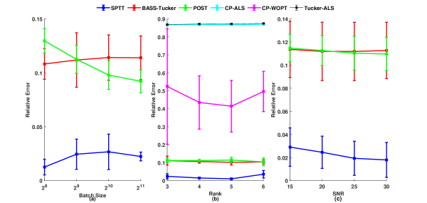
Figure 2: Predictive performance of synthetic data under different conditions.

In addition, we evaluate the running predictive performance of SPTT. We fix the batch size $S=512$, $\operatorname{SNR}=20$, and gradually feed the training set $\{B_{1},B_{2},\ldots,B_{t_{\max}}\}$ to SPTT, BASS-Tucker and POST. Two cases ($R=3,\,5$) are considered to test the prediction accuracy after each data batch is used. The corresponding running relative error is shown in Fig. 3. As we can see, our SPTT algorithm beats POST and BASS-Tucker since the first data batch, which demonstrates the accuracy and efficiency of our algorithm.

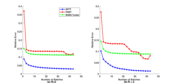
Figure 3: The running predictive performance of synthetic data.

4.2 Real-world applications

We evaluate the SPPT algorithm on the following three datasets: (1) Alog [29], a three-mode (user, action, resource) tensor, of size $200\times 100\times 200$, including $0.66\%$ observed entries. It represents three-way management operations. (2) Carphone [30], a three-mode (length, width, frames) of video data size $144\times 176\times 180$, contains $0.5\%$ nonzeros entries. (3) Flow injection, a three-mode (samples, wavelengths, times) tensor of size $12\times 100\times 89$, is exacted from a flow injection analysis system and includes $21360$ nonzero entries.

Set $M=100$ in Algorithm 1 and the initial TT-cores with TT-ranks as $(1,R,R,R,1)$. For maximum iteration number and initialization of all the completing approaches, we use their default settings. We compare the relative reconstruction error $\epsilon$ defined in (29) under different batch size $S$ and different initial rank $R$. We randomly split the observed entries of Alog into $75\%$ for training and $25\%$ for test and the other two datasets $10\%$ entries for test. For POST, SPTT and BASS-Tucker, we randomly partitioned the training entries into a stream of small batches according to batch size $S$. For static decomposition algorithm CP-ALS, CP-WOPT and Tucker-ALS, we input the whole data. The average relative error and standard deviation are reported in Fig. 4. In Fig. 4 (a)-(c), we fix the batch size $S=512$ and show how the predictive performance of each method varied with different rank $R=\{3,4,5,6\}$. The bigger the rank, the more expensive for SPTT to factorize each batch. It can be seen form Fig. 4 (c), as the initial rank $R$ increase from $3$ to $5$, the relative error of SPTT gradually increase and finally close to the relative error of POST. Hence this setting examined the trade-off between the accuracy and computational complexity. To test the capacity of decomposition algorithm on different batch size, we fix the rank $R=3$, and examine the performance with different choices of batch sizes $B=\{2^{8},2^{9},2^{10},2^{11}\}$ in Fig. 4 (d)-(f). As we can see, SPTT outperforms BASS-Tucker, POST and static decomposition methods in three datasets, especially in dataset Carphone.

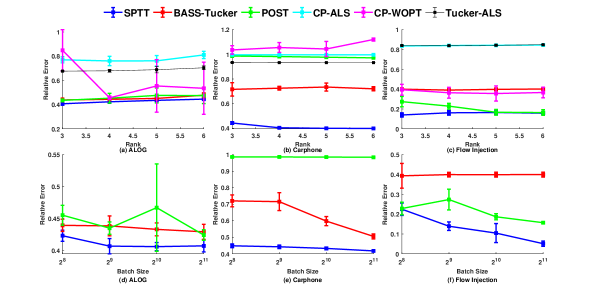
Figure 4: Predictive performance with different rank(top row) and streaming batch size (bottom row).

We then evaluate the running predictive performance of SPTT. We fix the batch size $S=512$, and continuously feed the training set to SPTT, BASS-Tucker and POST. For the three datasets, we consider two cases, i.e. $R=3$ and $R=5$ to test the prediction accuracy after each data batch is used. The running relative error is shown in Fig. 3. In all the cases, when the number of batches is small, POST or BASS-Tucker may performs better than SPTT. However, as the data streams, SPTT beats POST and BASS-Tucker gradually.

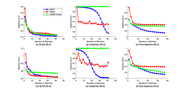
Figure 5: The running predictive performance in real-world applications.

5 Conclusions

In this paper, we propose a novel and efficient algorithm, namely SPTT, to discover latent factors from streaming data from high-order tensor and predict missing values. We introduce a simple probabilistic TT model for data denosing and decomposition. Under the SVI framework, we develop posterior inference for TT-cores and the inverse of noise variance. We demonstrate that our SPTT algorithm can produce accurate predictions on streaming data. For future work, we are interested in develop a sparse strategy based on SPTT to further prevent overfitting and enhance scalability.

References

- [1] E. Frolov, I. Oseledets, Tensor methods and recommender systems, Wiley Interdisciplinary Reviews: Data Mining and Knowledge Discovery 7 (3) (2017) e1201.
- [2] Y. Zhang, X. Bi, N. Tang, A. Qu, Dynamic tensor recommender systems, The Journal of Machine Learning Research 22 (1) (2021) 3032–3066.
- [3] Y. Panagakis, J. Kossaifi, G. G. Chrysos, J. Oldfield, M. A. Nicolaou, A. Anandkumar, S. Zafeiriou, Tensor methods in computer vision and deep learning, Proceedings of the IEEE 109 (5) (2021) 863–890.
-
[4]
M. Filippi, M. Cercignani, M. Inglese, M. Horsfield, G. Comi,
Diffusion tensor magnetic
resonance imaging in multiple sclerosis, Neurology 56 (3) (2001) 304–311.
arXiv:https://n.neurology.org/content/56/3/304.full.pdf, doi:10.1212/WNL.56.3.304.
URL https://n.neurology.org/content/56/3/304 -
[5]
K. Tang, Q. Liao,
Rank
adaptive tensor recovery based model reduction for partial differential
equations with high-dimensional random inputs, Journal of Computational
Physics 409 (2020) 109326.
doi:https://doi.org/10.1016/j.jcp.2020.109326.
URL https://www.sciencedirect.com/science/article/pii/S0021999120301005 - [6] Y. Ji, Q. Wang, X. Li, J. Liu, A survey on tensor techniques and applications in machine learning, IEEE Access 7 (2019) 162950–162990.
- [7] Y. Yu, G. Zhou, N. Zheng, Y. Qiu, S. Xie, Q. Zhao, Graph-regularized non-negative tensor-ring decomposition for multiway representation learning, IEEE Transactions on Cybernetics (2022) 1–14doi:10.1109/TCYB.2022.3157133.
- [8] M. Mørup, Applications of tensor (multiway array) factorizations and decompositions in data mining, Wiley Interdisciplinary Reviews: Data Mining and Knowledge Discovery 1 (1) (2011) 24–40.
- [9] N. D. Sidiropoulos, L. De Lathauwer, X. Fu, K. Huang, E. E. Papalexakis, C. Faloutsos, Tensor decomposition for signal processing and machine learning, IEEE Transactions on Signal Processing 65 (13) (2017) 3551–3582.
- [10] R. A. Harshman, et al., Foundations of the parafac procedure: Models and conditions for an” explanatory” multimodal factor analysis (1970).
- [11] R. Bro, Parafac. tutorial and applications, Chemometrics and intelligent laboratory systems 38 (2) (1997) 149–171.
- [12] J. Jiang, F. Sanogo, C. Navasca, Low-cp-rank tensor completion via practical regularization, Journal of Scientific Computing 91 (1) (2022) 18.
- [13] L. R. Tucker, Some mathematical notes on three-mode factor analysis, Psychometrika 31 (3) (1966) 279–311.
- [14] C. Xiao, C. Yang, M. Li, Efficient alternating least squares algorithms for low multilinear rank approximation of tensors, Journal of Scientific Computing 87 (2021) 1–25.
- [15] T. G. Kolda, B. W. Bader, Tensor decompositions and applications, SIAM review 51 (3) (2009) 455–500.
- [16] I. V. Oseledets, Tensor-train decomposition, SIAM Journal on Scientific Computing 33 (5) (2011) 2295–2317.
- [17] R. Roy, G. A. Rao, Survey on pre-processing web log files in web usage mining, International Journal of Advanced Science and Technology 29 (3 Special Issue) (2020) 682–691.
- [18] D. Koutra, E. E. Papalexakis, C. Faloutsos, Tensorsplat: Spotting latent anomalies in time, in: 2012 16th Panhellenic Conference on Informatics, IEEE, 2012, pp. 144–149.
- [19] Y. Du, Y. Zheng, K.-c. Lee, S. Zhe, Probabilistic streaming tensor decomposition, in: 2018 IEEE International Conference on Data Mining (ICDM), IEEE, 2018, pp. 99–108.
-
[20]
S. Fang, R. M. Kirby, S. Zhe,
Bayesian streaming
sparse tucker decomposition, in: C. de Campos, M. H. Maathuis (Eds.),
Proceedings of the Thirty-Seventh Conference on Uncertainty in Artificial
Intelligence, Vol. 161 of Proceedings of Machine Learning Research, PMLR,
2021, pp. 558–567.
URL https://proceedings.mlr.press/v161/fang21b.html - [21] L. Xu, L. Cheng, N. Wong, Y.-C. Wu, Probabilistic tensor train decomposition with automatic rank determination from noisy data, in: 2021 IEEE Statistical Signal Processing Workshop (SSP), 2021, pp. 461–465. doi:10.1109/SSP49050.2021.9513808.
- [22] W. Wang, V. Aggarwal, S. Aeron, Tensor completion by alternating minimization under the tensor train (tt) model, arXiv preprint arXiv:1609.05587 (2016).
-
[23]
L. Yuan, Q. Zhao, L. Gui, J. Cao,
High-order
tensor completion via gradient-based optimization under tensor train format,
Signal Processing: Image Communication 73 (2019) 53–61, tensor Image
Processing.
doi:https://doi.org/10.1016/j.image.2018.11.012.
URL https://www.sciencedirect.com/science/article/pii/S0923596518311081 - [24] T. Broderick, N. Boyd, A. Wibisono, A. C. Wilson, M. I. Jordan, Streaming variational bayes, Advances in neural information processing systems 26 (2013).
- [25] M. J. Wainwright, M. I. Jordan, et al., Graphical models, exponential families, and variational inference, Foundations and Trends® in Machine Learning 1 (1–2) (2008) 1–305.
- [26] T. G. K. Brett W. Bader, et al., Tensor toolbox for matlab, version 3.4, www.tensortoolbox.org (Sep. 2022).
- [27] E. Acar, D. M. Dunlavy, T. G. Kolda, M. Mørup, Scalable tensor factorizations for incomplete data, Chemometrics and Intelligent Laboratory Systems 106 (1) (2011) 41–56.
- [28] L. De Lathauwer, B. De Moor, J. Vandewalle, On the best rank-1 and rank-(r 1, r 2,…, rn) approximation of higher-order tensors, SIAM journal on Matrix Analysis and Applications 21 (4) (2000) 1324–1342.
- [29] S. Zhe, K. Zhang, P. Wang, K.-c. Lee, Z. Xu, Y. Qi, Z. Ghahramani, Distributed flexible nonlinear tensor factorization, Advances in neural information processing systems 29 (2016).
- [30] G. Song, M. K. Ng, X. Zhang, Robust tensor completion using transformed tensor singular value decomposition, Numerical Linear Algebra with Applications 27 (3) (2020) e2299.