Third sound detectors in accelerated motion

Abstract

An accelerated observer moving through empty space sees particles appearing and disappearing, while an observer with a constant velocity does not register any particles. This phenomenon, generally known as the Unruh effect, relies on an initial vacuum state, thereby unifying the experience of all inertial observers. We propose an experiment to probe this observer-dependent detector response, using a laser beam in circular motion as a local detector of superfluid helium-4 surface modes or third sound waves. To assess experimental feasibility, we develop a theoretical framework to include a non-zero temperature initial state. We find that an acceleration-dependent signal persists, independent of the initial temperature. By introducing a signal-to-noise measure we show that observing this signal is within experimental reach.

Introduction.—

One of the hardest-to-detect yet crucial predictions arising at the interface of quantum physics and relativity is the Unruh effect [1]. It predicts that observers in accelerated and inertial motion perceive empty space differently. While the latter sees nothing, the observer accelerating through the quantum vacuum will experience particles popping in and out of existence with a thermal spectrum characterized by a temperature proportional to its acceleration. This disparity is fundamental for our understanding of the interplay between quantum and relativistic aspects of the Universe.

Two obstacles stand in the way of the experimental observation of the Unruh effect. The first is a technical challenge in reaching prohibitively large accelerations for an appreciable temperature. The more fundamental and as yet unexamined issue is the crucial dependence on the precise properties only provided by the quantum vacuum state, which unify the perception of all non-accelerating observers travelling at any constant velocity. For an initial state differing from the quantum vacuum, such as a thermal state, this agreement between inertial observers is tainted by a Doppler-shifted spectrum according to their velocities [2].

In the present Letter, we tackle these two issues at hand. We devise a quantum simulator in superfluid helium where the phenomenon of observer-dependence persists, and a high ambient temperature can be seized as an experimental advantage by allowing the scanning of a wide range of acceleration temperatures. Specifically, we develop a quantitative framework for both controlling this initial thermality and distinguishing between the inertial (Doppler) and acceleration (Unruh) signatures. We further show that a laser can be used as a continuous detector to extract this acceleration-dependent signal.

An accelerated particle detector on a circular trajectory can be constructed using a localized laser beam interacting with an ultracold atoms system [3, 4]. Such gravity simulators are accessible playing fields with controllable parameter spaces and have been successful in probing fundamental phenomena [5, 6, 7]. We show that long-wavelength perturbations on the surface of thin film superfluid helium-$4$, commonly referred to as third sound [8], obey an effective quantum field theory [9]. In investigating the dynamics of superfluids, including both surface excitations [10, 11, 12, 13, 14, 15] and acoustic phonons [16, 17, 18, 19], optomechanical systems have been effectively utilised with remarkable precision.

Using a laser as a probe field, we show height fluctuations $\delta h$ on the surface of superfluid helium are transduced into phase fluctuations $\psi$ in the laser,

$$\psi_{\delta h}~{}\approx~{}\tfrac{1}{2}(n^{2}-1)k_{L}\delta h\,,$$ (1)

with index of refraction $n$ and laser wavevector $k_{L}$. Using our proposed setup in Figure 1, phase-referenced (homodyne [20, 21]) photodetection retrieves the phase spectrum and with it a signature of the Unruh effect.

In view of the central role of acceleration, we introduce the difference spectrum: a measure of the observability of acceleration-dependence in the detector response. This quantity is obtained by subtracting a purely velocity-dependent contribution arising from inertial motion through a thermal bath. We demonstrate that the difference spectrum is operationally measurable and present a signal-to-noise analysis indicating that it is observable. As such, our considerations of a realistic thermal initial state are crucial in the experimental realization of the Unruh effect.

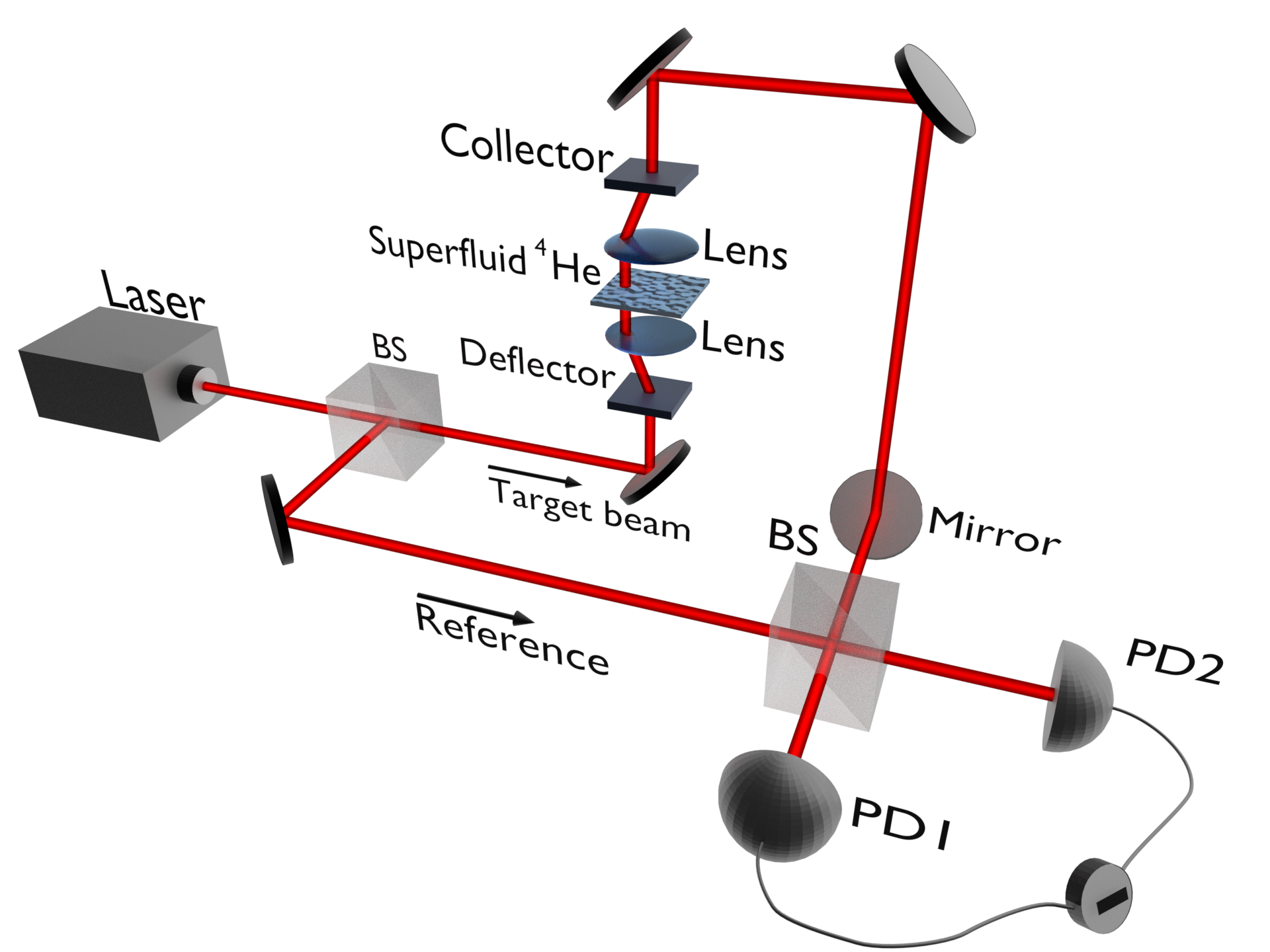
Figure 1: Experimental setup. A beam splitter (BS) separates the input laser into two arms, namely a target and a reference. A deflector-lens configuration moves the target beam on a circular trajectory through the superfluid helium sample. After the sample, a lens-collector combination, followed by a series of mirrors, brings the beam back to a static path and lead it to a second beam splitter (BS), where the target and reference arms are combined. The resulting beams are detected at two photodiodes (PD1) and (PD2).

Thin film superfluid helium-$4$.—

We begin by deriving the interfacial dynamics of superfluid helium-$4$ using Landau’s two-fluid model [22, 23] as a basis. This model states that below a critical temperature of $2.17\,\mathrm{K}$ (the lambda-point), helium-$4$ can be decomposed into a normal component and a superfluid component. We show that in a certain regime, the dynamics of classical height fluctuations $\delta h$ of the superfluid component can be effectively described by the $(2+1)-$dimensional Klein-Gordon equation. Owing to the linearity of the Klein-Gordon equation, the quantized height fluctuations $\delta\hat{h}$ obey the same effective field theory. Upon canonical quantization, the height field $\rho\delta\hat{h}$ and the velocity potential $\hat{\phi}$ become non-commuting variables and the experimental estimates later will follow from this quantization.

When deriving the equations of motion (see Supplemental Material for detailed derivation), we work under several assumptions. First, we will operate at low temperatures (below $500~{}\mathrm{mK}$), below which the superfluid component will dominate [24, 23], and we can neglect contributions from the normal component altogether, as well evaporation and recondensation of the superfluid [8]. This assumption also means that the saturated helium vapour pressure is approximately zero, and the pressure gradient originating from this interaction will vanish [25]. In addition, we will work in the isothermal limit, assuming that there is no heat transfer in the system due to wave propagation, thereby ignoring temperature gradients. Our final assumption is that we consider saturated thin films of helium-$4$ (i.e. height $h_{0}>10\,\mathrm{nm}$), at which thickness the superfluid component can form surface waves, which propagate independently of a stationary normal component - this is referred to as third sound [8, 26]. Given the film thickness is orders of magnitude larger than a few atomic layers, the superfluid helium-$4$ can be considered incompressible [27].

Under the aforementioned assumptions, we show in the Supplemental Material that the dynamics of the fluid components can be effectively linearized at the superfluid surface for small thickness perturbations $\delta h(t,\bm{x})=h(t,\bm{x})-h_{0}$. The result of this linearization is a wave equation for height fluctuations $\delta h$,

$$\nabla^{2}\delta h~{}=~{}\frac{1}{h_{0}g}\partial^{2}_{t}\delta h-\frac{\sigma}{g\rho}\nabla^{2}(\nabla^{2}\delta h)\;,$$ (2)

where $\sigma$ is the surface tension of superfluid helium-$4$. The effective gravity $g$ contains a contribution due to gravity $g_{0}$ and due to van der Waals interactions of the fluid with the substrate material via the coupling constant $\alpha_{vdW}$. For thin films, gravity is negligible compared to the van der Waals contribution, and the effective gravitational coupling is $g~{}=~{}g_{0}+3\alpha_{vdW}/h_{0}^{4}~{}\approx~{}3\alpha_{vdW}/h_{0}^{4}$ [28, 29]. The dispersion relation arising from (2) is of the form $\omega^{2}=h_{0}(g-\sigma k^{2}/\rho)k^{2}$. We consider the long-wavelength limit wherein the effective gravity dominates capillary effects, $\sigma k^{2}\ll g\rho$. In this case, the surface wave dispersion can be linearized with the third sound speed given by [30, 28]

$$\left(c_{3}\right)^{2}~{}=~{}\omega^{2}(k)k^{-2}\approx 3\alpha_{vdW}h_{0}^{-3}\;.$$ (3)

In this thin-film, nondispersive limit, (2) is the equation of motion for $\delta h(t,\bm{x})$ with corresponding Lagrangian

$$\mathcal{L}_{\text{fluid}}~{}=~{}\left|\partial_{t}\delta h\right|^{2}-c_{3}^{2}\left|\nabla\delta h\right|^{2}\;.$$ (4)

In this limit, we have that the height fluctuations $\delta h$ obey a Klein-Gordon equation with propagation speed $c_{3}$ with a linear dispersion $\omega=c_{3}k$. This is identical in form to the equations governing a quantum scalar field, used in the quantum field theoretical (QFT) derivation of the Unruh effect. This correspondence laid the groundwork for the birth of analogue gravity [31] and we appeal to it to motivate this work.

Lasers as local detectors of interface fluctuations.—

For a $(3+1)-$dimensional electromagnetic field, propagating in the $z$-direction with only one polarisation, we can express the electromagnetic potential as $A(t,z)=A_{0}\cos\left(\omega_{L}t-k_{L}z+\psi(t,z)\right)$. Before interaction with the superfluid helium-4, the quantized field $\psi$ is electromagnetic noise. We take the background laser field to be a plane wave, $A_{0}\cos(\omega_{L}t-k_{L}z)$, and the perturbation $\psi(t,z)$ to be a real field describing the phase fluctuations of the laser. By linearizing the standard electromagnetic Lagrangian in terms of small phase perturbations and after an appropriate rescaling of $\psi$ discussed in the Supplemental Material, we obtain

$$\mathcal{L}_{\text{em}}~{}=~{}\frac{1}{2\mu_{0}}\left(\frac{1}{c^{2}}\left(\partial_{t}\psi(t,z)\right)^{2}-\left(\partial_{z}\psi(t,z)\right)^{2}\right)\;,$$ (5)

where $\mu_{0}$ is the vacuum permeability and $c$ is the speed of light in vacuum.

When the laser beam passes through the superfluid, the atoms will react by forming dipoles according to their polarizabilities $\alpha$. Assuming the laser is sufficiently detuned from atomic resonances, $\alpha$ can be taken to be real and the superfluid-light interaction can be calculated within a semiclassical model in the framework of macroscopic electrodynamics. To shorten the notation in the following, $\alpha$ refers to the real part of the polarizability. The interaction between the superfluid and the laser is

$$\mathcal{L}_{\text{int}}~{}=~{}\tfrac{1}{2}\alpha\rho_{N}\left(\partial_{t}A\right)^{2}\;,$$ (6)

with $\rho_{N}$ the $3\mathrm{D}$ number density of helium-$4$ [32]. Using the above ansatz for $A$, this Lagrangian (6) can be expanded in small $\psi$. In the Supplemental Material, we derive the equation of motion for the laser phase localized to the trajectory $\bm{x}=\bm{X}(t)$ at the surface, where we will consider the interaction to be localized to a region on the free surface of the superfluid, lying on a circular trajectory with radius $R>0$ and angular frequency $\Omega>0$. This path can be parametrized as $\bm{X}(t)=(R\cos(\Omega t),R\sin(\Omega t))$. The equation of motion reads

$$\Box\psi(t,z)=-\alpha\rho_{N}\omega_{L}\mu_{0}\partial_{t}\delta h(t,\bm{X}(t))\delta(z-h_{0})\,,$$ (7)

where $\Box=(-c_{\mathrm{eff}}^{-2}\partial_{t}^{2}+\partial_{z}^{2})$ is the wave operator and $c_{\mathrm{eff}}$ is the effective speed of light, which models the effective slow-down of light through the superfluid via the electrostrictive interaction and is obtained from the interaction Lagrangian (6) in the Supplemental Material.

The laser phase equation of motion has a contribution from the height fluctuations and the equation of motion for the height fluctuations will have a contribution from the laser field, a phenomenon known as back action. In the limit of negligible back action of the laser phase on the height, we solve (7) exactly in the Supplemental Material,

$$\psi(t,z)~{}=~{}\psi_{0}(t,z)-\tfrac{1}{2}\alpha\rho_{N}\omega_{L}\mu_{0}c_{\mathrm{eff}}\delta h(\tau,\bm{X}(\tau)),$$ (8)

where $\tau=t-|z-h_{0}|/c_{\mathrm{eff}}$. It is then clear that the laser phase contains a contribution from the height fluctuations. We discuss in the Supplemental Material how this contribution can be seen as the laser acting as a detector for height fluctuations along the interaction trajectory. The phase fluctuation for weak interactions attributable to the height fluctuations given by (8) can be written as

$$\psi_{\delta h}~{}=~{}\tfrac{1}{2}\alpha\rho_{N}\omega_{L}c_{\mathrm{eff}}\mu_{0}\delta h~{}=~{}\tfrac{1}{2n}(n^{2}-1)k_{L}\delta h\,,$$ (9)

in terms of an index of refraction $n$ as defined by

$$n~{}=~{}c/c_{\text{eff}}~{}=~{}\sqrt{1+\alpha\rho_{N}/\epsilon_{0}}\;,$$ (10)

where $\epsilon_{0}$ is the vacuum permittivity. Note that (9) differs from the phase associated with an optical path-length difference and is approximated in (1).

The interaction (6) generates correlations, as the laser phase samples fluctuations of the helium surface along the interaction trajectory. As a result, the characteristic trajectory-dependence as expected from the Unruh effect is encoded in laser phase correlations of the outgoing laser. By recombining the laser after interaction with a reference beam split off from the initial laser, as illustrated by the homodyne arrangement in Figure 1, one can vary the phase along the reference arm to convert phase fluctuations to intensity fluctuations for readout at photodiodes $1$ and $2$.

Experimental estimates.—

The relevant homodyne spectrum in the present setup is characterized by the power spectral density (PSD) $S_{\psi}(\omega)$ of quantum phase fluctuations in the laser. The solution (8) shows that the power spectrum contains a contribution from the height fluctuations on the surface of the superfluid helium. Our central aim is to identify in this contribution the effect due to the circular acceleration of the laser beam. The acceleration effect has been shown to be approximately thermal [33, 34, 35] and is characterised over most of the parameter space by an approximate Unruh temperature $T_{U}$, given by [3, 36]

$$k_{B}T_{U}~{}=~{}\frac{\gamma_{s}v^{2}}{2\pi c_{3}^{2}}\hbar\Omega_{R}\;,$$ (11)

where $c_{3}$ is the third sound speed (3), $v$ is the orbital speed of the laser dot on the helium surface, $\Omega_{R}=c_{3}/R$ and $\gamma_{s}=(1-v^{2}/c_{3}^{2})^{-1/2}$. We shall show that the circular acceleration effect is identifiable in the PSD even when $T_{U}$ is smaller than the ambient temperature in the helium.

Having established the prerequisite formalism, we move to discuss experimentally realizable scenarios. Our gravity simulator enables tuning the third speed of sound in superfluid helium-$4$. To do so, we consider a typical saturated film thickness of $h_{0}=100\,\textrm{nm}$, which are within experimental reach [30, 11, 37]. The resulting speed of sound is $c_{3}~{}\approx~{}8.8\times 10^{-2}\;\textrm{m}\,\textrm{s}^{-1}$. In order to achieve a “relativistic” speed of $v=0.95c_{3}$ with readily attainable rotation frequency in the hundreds of Hertz, we specify a trajectory radius of $60\,\mu\textrm{m}$ (corresponding to $\Omega/(2\pi)\approx 222\,\mathrm{Hz}$), for which we have the approximate Unruh temperature (11) $T_{U}\approx 5\,\textrm{nK}$. As standard superfluid helium-$4$ operating temperatures are in the millikelvin to kelvin region [23, 11], i.e., orders of magnitude above $T_{U}$, the laser phase will pick up thermal fluctuations of the surface even with a static laser.

We choose to stay at the lower end of the typical temperature range, with $T=10\,\mathrm{mK}$, in line with our model assumptions. Hence, the relatively high ambient temperature in helium systems motivates the inclusion of this non-vanishing $T$ in the detector response function $\mathcal{F}(\omega;T)$ [2], which is the PSD of superfluid height fluctuations sampled by the detector. Our analogue detector interacts along a circular trajectory with an effective relativistic field prepared in a thermal state at the ambient temperature $T$. Since $T\gg T_{U}$, the majority of the detector response will pertain to thermal fluctuations, rather than the vacuum. However, as mentioned in the introduction, the nonzero acceleration of the detector will indeed have an effect on these thermal fluctuations.

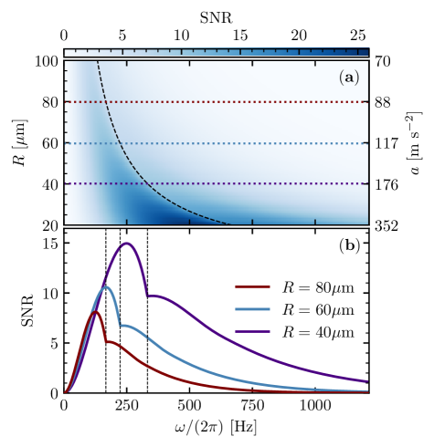
Figure 2: SNR (14) for $\mathcal{N}=10^{5}$ realizations with a bandwidth of $\mathcal{B}=1$. Superfluid temperature $T=10\,\mathrm{mK}$, speed $v=0.95c_{3}$ and horizontal $\omega$-axis all apply to plots (a) and (b) equally. (a) Computed SNR for orbital radii $20\,\mu\mathrm{m}\leq R\leq 100\,\mu\mathrm{m}$. Dashed black curve denotes angular frequency $\Omega$ of the laser’s trajectory. Purple, blue and dark red dotted lines are lines of constant radii, whose SNRs are displayed in (b). (b) Computed SNR for constant radial slices in (a). Vertical black dashed lines represent angular frequencies for $R=40\,\mu\mathrm{m}$ (far right), $60\,\mu\mathrm{m}$, and $80\,\mu\mathrm{m}$ (far left).

Figure 3: SNR (14) for $\mathcal{N}=10^{5}$ realizations with a bandwidth of $\mathcal{B}=1$ and orbital radius $R=60\,\mu\mathrm{m}$. Horizontal $\omega$-axis applies to plots (a) and (b) equally. Dashed vertical black line in both (a) and (b) denotes angular frequency $\Omega$ of the laser’s trajectory. (a) Computed SNR for superfluid at temperatures $1\,\mu\mathrm{K}\leq T\leq 1\,\mathrm{K}$. Purple, blue and dark red dotted lines are lines of constant superfluid temperature, whose SNRs are displayed in (b). (b) Computed SNR for constant temperature slices in (a).

The phase PSD is given (cf. Supplemental Material) in terms of the response function $\mathcal{F}(\omega;T)$ and a shot noise term $\sigma_{\mathrm{sn}}^{2}$ as

$$S_{\psi}(\omega)=\kappa\mathcal{F}(\omega;T)+\sigma_{\mathrm{sn}}^{2}\,.$$ (12)

The coupling $\kappa$ is determined by (9) and is given explicitly in the Supplemental Material, allowing us to map between the QFT formalism [2] and the hydrodynamical formalism. We obtain this result in the nondispersive regime with threshold $\hbar\omega\ll\tfrac{1}{2}\hbar c_{3}\sqrt{\rho g/\sigma}$. For a height of $100\,\mathrm{nm}$, $\tfrac{1}{2}\hbar c_{3}\sqrt{\rho g/\sigma}\approx(2\pi\hbar)1.2\,\mathrm{kHz}$.

In order to isolate acceleration-dependence of the detector response carried by our phase signal, we define the difference spectrum $S_{\delta}(\omega)$ [2], given by

$$S_{\delta}(\omega)~{}=~{}S_{\psi}(\omega)-\sigma_{\mathrm{sn}}^{2}-\kappa\mathcal{F}_{\mathrm{Lin}}(\omega;T)\,,$$ (13)

where shot noise-induced phase fluctuations are approximated as Gaussian with variance $\sigma^{2}_{\mathrm{sn}}=\hbar\omega_{L}/P$, assumed independent of frequency within the measurement band. In our calculations, we assume a laser power $P=0.5\,\mathrm{mW}$, which is low enough to prevent the evaporation of the superfluid helium-$4$, with wavelength $\lambda_{L}=700\,\mathrm{nm}$ and beam width $r_{0}=10\,\mu\mathrm{m}$. The quantity $\mathcal{F}_{\mathrm{Lin}}(\omega;T)$ in (13) is operationally measurable from the circular-motion response (12) alone, as we show in the Supplemental Material. The difference spectrum (13) is a measure of the deviation of response from that of a detector in linear motion at the same constant speed $v$ (characterized by the response $\mathcal{F}_{\mathrm{Lin}}(\omega;T)$), which extracts acceleration-dependent effects present in the phase PSD.

To determine the feasibility of measuring the difference spectrum, we use the signal-to-noise (SNR) quantifier

$$\mathrm{SNR}~{}=~{}\sqrt{\frac{\mathcal{N}\mathcal{B}}{2}}\frac{S_{\delta}(\omega)}{\sigma^{2}_{\mathrm{sn}}\sqrt{1+2\frac{S_{\delta}(\omega)}{\sigma^{2}_{\mathrm{sn}}}+2\frac{S_{\delta}^{2}(\omega)}{\sigma^{4}_{\mathrm{sn}}}}}\,,$$ (14)

where $\mathcal{N}$ is the number of realizations and $\mathcal{B}$ is the resolution bandwidth in units of the measurement bandwidth [3]. Figures 2 and 3 explore the wider parameter space for viable experimental implementation. For a constant velocity $v$, the acceleration $a=v^{2}R^{-1}$ is inversely proportional to the orbital radius $R$; hence, Figure 2 can be interpreted in terms of the Unruh effect: the signal increases with acceleration. The blue curve in Figures 2 (b) and 3 (b) represent the common intersection of the two parameter searches. Figure 3 shows that the acceleration-dependent features are amplified by an increase in the temperature of superfluid helium. This is also noted in our supporting paper [2], wherein this increase in signal with increasing ambient temperature is interpreted as a lowering in the effective temperature experienced by the detector.

Conclusion.—

We have proposed an experimental setup that exhibits an analogue of the circular-motion Unruh effect in thin film superfluid helium-4. Using a continuous probing field (i.e. a laser) as a detector, one can sample surface fluctuations along an accelerated (circular) interaction trajectory. In the third sound regime, the surface fluctuations behave as an effective relativistic field, and the detector response function extracted from the laser phase carries information about the acceleration along the circular path. We note that the analysis presented here does not account for either finite-size effects or the induced noise in the superfluid due to the electrostrictive drag of the laser. We leave an in-depth examination of these effects to future work.

Using a signal-to-noise measure derived from the principle of extracting only acceleration-dependent effects, we explored experimentally viable superfluid helium-4 temperatures and rotating detector radii. The results in Figures 2 and 3 correspond to a film thickness of $100\,\mathrm{nm}$ and show the behaviour of the system in the high-temperature limit, $k_{B}T\gg\hbar\omega$, for frequencies $\omega$ within the nondispersive band. By reducing the film thickness, one can shift the SNR peak - and broaden the nondispersive band - to high enough frequencies for vacuum effects to potentially be visible (i.e. $k_{B}T\lesssim\hbar\omega$).

We re-emphasise that the initial state in our helium-$4$ system is thermal, and significantly different from the vacuum that features in textbook descriptions of the Unruh effect, but we found that an acceleration-dependent response persists, with the SNR increasing with acceleration. Furthermore, we showed that the Unruh signature is amplified as the temperature of the superfluid helium-$4$ increases. In this way, our proposed experimental setup, framework, and analysis are pivotal and provide a stepwise approach, enabling the immediate experimental exploration of the circular-motion Unruh effect.

We thank Jörg Schmiedmayer, Bill Unruh, Sebastian Erne, and other members of the Quantum Sensors discussion group, for helpful discussions. We thank Radivoje Prizia for producing the $3\mathrm{D}$ schematic in Figure 1. We acknowledge support provided by the Leverhulme Research Leadership Award (RL-2019- 020), the Royal Society University Research Fellowship (UF120112, UF150140, URF\R\211009, RF\ERE\210198) and the Royal Society Enhancements Awards and Grants (RGF\EA\180286, RGF\EA\181015, RGF\EA\180099, RGF\R1\180059, RPG\2016\186), and partial support by the Science and Technology Facilities Council (Theory Consolidated Grant ST/P000703/1), the Science and Technology Facilities Council on Quantum Simulators for Fundamental Physics (ST/T006900/1, ST/T005998/1) as part of the UKRI Quantum Technologies for Fundamental Physics programme. The work of JL was supported by United Kingdom Research and Innovation Science and Technology Facilities Council [grant number ST/S002227/1]. For the purpose of open access, the authors have applied a CC BY public copyright licence to any Author Accepted Manuscript version arising.

I Supplemental Material

I.1 Experimental Parameters

Parameter	Value
Helium-4
Film height, $h_{0}$	$100~{}\textrm{nm}$
Mass density, $\rho$	$145~{}\textrm{kg}\,\textrm{m}^{-3}$
Surface tension, $\sigma$	$37.9\times 10^{-5}~{}\textrm{J}\,\textrm{m}^{-2}$
Van der Waals const., $\alpha_{vdW}$	$2.6\times 10^{-24}~{}\mathrm{m}^{5}\mathrm{s}^{-2}$
Index of refraction, $n$	1.025

Table 1: Experimental parameters for helium-4. The van der Waals constant is given for a quartz substrate [30]; for other materials, $\alpha_{vdW}$ would be of the same order of magnitude.

I.2 Linearization of Superfluid Interfacial Dynamics

Consider a film of superfluid helium confined in a container with a flat bottom at $z=0$ and a free surface at $z=h(t,\bm{x})$. We assume a constant, uniform density $\rho$ and align the vertical axis such that $\mathbf{g}=-\nabla(gz)$. Imposing the no-penetration boundary condition at $z=0$ and the kinematic boundary condition at the free surface allows the linearization of the fluid dynamical equations in terms of small height perturbations $\delta h(t,\bm{x})=h(t,\bm{x})-h_{0}$ [26]. The governing equations can be further simplified by the assumptions we stated before. The velocity field of the superfluid component $\bm{v}_{s}$ is assumed to be irrotational such that $\nabla\times\bm{v}_{s}=0$, and therefore $\bm{v}_{s}=-\nabla\phi$.

We first impose the kinematic boundary condition at the interface between helium and helium-vapour at $z=h(t,\bm{x})$, and the no-penetration boundary condition at $z=0$ for fluid components $v_{i}$, where $i=n$, $s$ corresponding to the normal and superfluid components respectively,

$$\partial_{z}v_{i}~{}=~{} 0\,,$$ (S1)

$$v_{z}~{}=~{} \partial_{t}h+\bm{v}\cdot\nabla h\,.$$ (S2)

These can be used to linearize the governing equations in terms of small height perturbations $\delta h(t,\bm{x})=h(t,\bm{x})-h_{0}$ [26]

$$\rho\partial_{t}\delta h+\rho h_{0}\bm{\nabla}\cdot\bm{v}_{s}+J_{m}^{vap}~{}=~{} 0\,,$$ (S3)

$$\partial_{t}\bm{v}_{s}+g\bm{\nabla}\delta h-\frac{\sigma}{\rho}\bm{\nabla}(\nabla^{2}\delta h)+\frac{1}{\rho}\bm{\nabla}p-s\bm{\nabla}T~{}=~{} 0\,,$$ (S4)

with $J_{m}^{vap}=\mathrm{d}m/\mathrm{d}t$ the mass variation due to evaporation and recondensation, $\sigma$ the surface tension and $s$ the entropy of the fluid. The interaction constant $g$ contains a contribution due to gravity and due to van der Waals interactions of the fluid with the substrate material. For thin films, the effective gravitational coupling is [28, 29]

$$g~{}=~{}g_{0}+3\frac{\alpha_{vdW}}{h^{4}}~{}\approx~{}3\frac{\alpha_{vdW}}{h^{4}}\,,$$ (S5)

with $g_{0}$ the usual acceleration due to gravity and $\alpha_{vdW}$ the van der Waals coupling. This approximation holds in thin films, where the effective gravity stems almost entirely from the van der Waals contribution.

Working within the isothermal limit, we can neglect the temperature gradient $\nabla T=0$ [8]. By considering low enough temperatures we can neglect the pressure gradient $\nabla p=0$, and the evaporation/recondensation on the surface $J_{m}^{vap}=0$ [8]. We can then simplify equations (S3) and (S4), which can then be combined into a wave equation for height fluctuations $\delta h$,

$$\nabla^{2}\delta h~{}=~{}\frac{1}{h_{0}g}\partial^{2}_{t}\delta h-\frac{\sigma}{g\rho}\nabla^{2}(\nabla^{2}\delta h)\;.$$ (S6)

In this limit, the speed of surface wave propagation is given by [30]

$$c_{3}^{2}~{}=~{}\frac{\omega^{2}(k)}{k^{2}}~{}=~{}\left(gh_{0}+\frac{1}{\rho}\sigma h_{0}k^{2}\right)\;.$$ (S7)

For thin films where the effective gravity dominates over capillary effects, i.e., $\sigma k^{2}\ll g\rho$ in (S7), the dispersion can be linearized $\omega(k)\approx\sqrt{gh_{0}}k$, with third sound speed

$$c_{3}~{}=~{}\sqrt{\frac{3\alpha_{vdW}}{h_{0}^{3}}}\;.$$ (S8)

I.3 Linearization of Electromagnetic Field

The free electromagnetic Lagrangian is given by

$$\mathcal{L}_{\text{em}}~{}=~{}-\frac{1}{4\mu_{0}}F_{\mu\nu}F^{\mu\nu}\;,$$ (S9)

where $F_{\mu\nu}=\partial_{\mu}A_{\nu}-\partial_{\nu}A_{\mu}$ and $\mu_{0}$ is the vacuum permeability. Working in the Coulomb gauge ($A_{t}=0$, $\nabla\cdot\bm{A}=0$) and with only one polarisation reduces this Lagrangian to

$$\mathcal{L}_{\text{em}}~{}=~{}\frac{1}{2\mu_{0}}\left(\frac{1}{c^{2}}\left(\partial_{t}A(t,z)\right)^{2}-\left(\partial_{z}A(t,z)\right)^{2}\right)\;,$$ (S10)

where $c$ is the speed of light in vacuum. We start linearizing the electromagnetic Lagrangian using the ansatz $A(t,z)=A_{0}\cos\left(\omega_{L}t-k_{L}z+\psi(t,z)\right)$. After averaging over fast oscillations to obtain $(\partial_{t}A)^{2}=A_{0}^{2}(\omega_{L}+\partial_{t}\psi)^{2}/2$ and $(\partial_{z}A)^{2}=A_{0}^{2}(-k_{L}+\partial_{z}\psi)^{2}/2$, the free electromagnetic Lagrangian for the perturbations $\psi(t,z)$ is then given by

$$\mathcal{L}_{\text{em}}~{}=~{}\frac{A_{0}^{2}}{4\mu_{0}}\left(\frac{1}{c^{2}}\left(\partial_{t}\psi(t,z)\right)^{2}-\left(\partial_{z}\psi(t,z)\right)^{2}\right)\;,$$ (S11)

since the terms linear in the first order derivatives contribute only as boundary terms. We can rescale $\psi$ such that it absorbs the constant factor $A_{0}/\sqrt{2}$ and obtain the standard form

$$\mathcal{L}_{\text{em}}~{}=~{}\frac{1}{2\mu_{0}}\left(\frac{1}{c^{2}}\left(\partial_{t}\psi(t,z)\right)^{2}-\left(\partial_{z}\psi(t,z)\right)^{2}\right)\;.$$ (S12)

I.4 Electromagnetic Interaction

Light-matter interaction for $\epsilon~{}\approx~{}\epsilon_{0}+\rho_{N}\alpha$ is given by the potential

$$V~{}=~{}-\frac{\alpha}{2}\rho_{N}(\partial_{t}A)^{2}\;,$$ (S13)

where $\rho_{N}$ is the number density of helium-4 and $\alpha$ is the polarizability. Using the ansatz $A(t,z)=A_{0}\cos(\omega_{L}-k_{L}z+\psi(t,z))$ and the same averaging argument as in the linearization of the electromagnetic field and after absorbing a factor of $A_{0}/\sqrt{2}$ into $\psi$, we can express the electromagnetic interaction as

$$\mathcal{L}_{\text{int}}~{}=~{}\frac{\alpha\rho_{N}}{2}\left(\frac{A_{0}\omega_{L}}{\sqrt{2}}+\partial_{t}\psi\right)^{2}\;.$$ (S14)

This can be split into three parts corresponding to powers in $\psi$. We momentarily drop the constant term. Then, the terms linear and quadratic in $\psi$ are given by

$$\mathcal{L}_{\text{int}}^{(1)}+\mathcal{L}_{\text{int}}^{(2)}~{}=~{}\alpha\rho_{N}\frac{A_{0}\omega_{L}}{\sqrt{2}}\partial_{t}\psi+\frac{\alpha\rho_{N}}{2}\left(\partial_{t}\psi\right)^{2}\;.$$ (S15)

The quadratic term contributes to the propagation speed of $\psi$, which can be seen by combining it with the time derivative in the free Lagrangian to obtain

$$\mathcal{L}_{\text{em}}~{}=~{}\left(\frac{1}{2\mu_{0}}\frac{1}{c^{2}}+\frac{\alpha\rho_{N}}{2}\right) \left(\partial_{t}\psi(t,z)\right)^{2}$$

$$-\frac{1}{2\mu_{0}}(\partial_{z}\psi(t,z))^{2}\,,$$ (S16)

$$~{}=~{}\frac{1}{2\mu_{0}}\left(\frac{1}{c^{2}}\left(1+\alpha\rho_{N}c^{2}\mu_{0}\right)\right. \left(\partial_{t}\psi(t,z)\right)^{2}$$

$$\left.-(\partial_{z}\psi(t,z)^{2})\right)\Big{)}\;.$$ (S17)

This defines an effective speed of light in the medium

$$\frac{1}{c_{\text{eff}}^{2}}~{}=~{}\frac{1}{c^{2}}\left(1+\frac{\alpha\rho_{N}}{\epsilon_{0}}\right)\;,$$ (S18)

when combined with the identity $c^{2}=(\mu_{0}\epsilon_{0})^{-1}$, where $\epsilon_{0}$ is the vacuum permittivity.

I.5 Equations of Motion

We consider now the equations of motion arising from the interaction term confined to the superfluid helium volume,

$$S_{int}~{}=~{}\int\mathrm{d}t\mathrm{d}^{2}\bm{x}\int_{0}^{h(t,\bm{x})}\mathrm{d}z\,\frac{\alpha\rho_{N}}{2}\left(\frac{A_{0}\omega_{L}}{\sqrt{2}}+\partial_{t}\psi\right)^{2}\,.$$ (S19)

Only the linear contribution to (S19) is relevant for the interaction as the quadratic part contributes to the effective speed of light (S18). Varying the linear part with respect to the phase field and momentarily dropping the argument of $h(t,\bm{x})$ yields [38],

$$\delta S_{int}~{}=~{} \int\mathrm{d}t\mathrm{d}^{2}\bm{x}\int_{0}^{h}\mathrm{d}z\,\frac{\alpha\rho_{N}}{\sqrt{2}}A_{0}\omega_{L}\partial_{t}\delta\psi\,,$$ (S20)

$$=~{} -\int\mathrm{d}t\mathrm{d}^{2}\bm{x}\,\frac{\alpha\rho_{N}}{\sqrt{2}}A_{0}\omega_{L}\partial_{t}(h)\left.\delta\psi\right|_{z=h}\,,$$ (S21)

$$=~{} -\frac{\alpha\rho_{N}}{\sqrt{2}}A_{0}\omega_{L}\int\mathrm{d}t\mathrm{d}^{2}\bm{x}\mathrm{d}z\,\partial_{t}(h)\delta(z-h)\delta\psi\,,$$ (S22)

where in the second inequality, we used the Leibniz integral rule with vanishing boundary terms and in the third equality, we rewrote the valuation $z=h(t,\bm{x})$ as an integral over $z$ with a delta function.

We consider perturbations of the height with respect to a constant background, $h(t,\bm{x})=h_{0}+\delta h(t,\bm{x})$, hence to first order, we find

$$\delta S_{int}~{}=~{}-\frac{\alpha\rho_{N}}{\sqrt{2}}A_{0}\omega_{L}\int\mathrm{d}t\mathrm{d}^{2}\bm{x}\mathrm{d}z\,(\partial_{t}\delta h)\delta(z-h_{0})\delta\psi\,.$$ (S23)

We absorb a factor of $A_{0}/\sqrt{2}$ into $\delta h(t,\bm{x})$ and introduce a factor of $\delta(\bm{x}-\bm{X}(t))$ to localize the interaction to the laser trajectory. We can then write the variation of the interaction part of the action as,

$$\delta S_{int}~{}=~{}- \alpha\rho_{N}\omega_{L}\int\mathrm{d}t\mathrm{d}^{2}\bm{x}\mathrm{d}z\,(\partial_{t}\delta h(t,\bm{x}))\delta\psi(t,z)$$

$$\times\delta(\bm{x}-\bm{X}(t))\delta(z-h_{0})\,.$$ (S24)

Variation of the entire action $S=S_{em}+S_{int}$ (where the free electromagnetic Lagrangian is given by (S17)) with respect to the laser phase field results in the equations of motion

$$-\frac{1}{c_{\mathrm{eff}}^{2}}\partial_{t}^{2}\psi(t,z) +\partial_{z}^{2}\psi(t,z)~{}=~{}$$

$$- \alpha\rho_{N}\omega_{L}\mu_{0}\partial_{t}\delta h(t,\bm{X}(t))\delta(z-h_{0})\,.$$ (S25)

The homogeneous part gives the solution $\psi_{0}(t,z)$, whereas the inhomogeneous part can be solved using the Green’s function for the operator $-c_{\mathrm{eff}}^{-2}\partial_{t}^{2}+\partial_{z}^{2}$, which is $G(t,z)=\frac{c_{\mathrm{eff}}}{2}\Theta(t-|z|/c_{\mathrm{eff}})$, where $\Theta(x)$ is the Heaviside function. This results in the solution

$$\psi(t,z)~{}=~{}\psi_{0}(t,z)-\tfrac{1}{2}\alpha\rho_{N}\omega_{L}\mu_{0}c_{\mathrm{eff}}\delta h(\tau,\bm{X}(\tau))\,,$$ (S26)

where $\tau=t-|z-h_{0}|/c_{\mathrm{eff}}$.

I.6 Field Theory

The system of equations in the isothermal limit

$$\rho\partial_{t}\delta h+\rho h_{0}\bm{\nabla}^{2}\phi~{}=~{} 0\,,$$ (S27)

$$\partial_{t}\phi+g\delta h~{}=~{} 0\,,$$ (S28)

can be derived with the Hamiltonian

$$\mathcal{H}~{}=~{}\frac{1}{2}\rho\left[h_{0}\left(\nabla\phi\right)^{2}+g\left(\delta h\right)^{2}\right]\;,$$ (S29)

and the equations of motion

$$\rho\partial_{t}\delta h~{}=~{} \frac{\delta\mathcal{H}}{\delta\phi}\;,$$ (S30)

$$\partial_{t}\phi~{}=~{} -\frac{1}{\rho}\frac{\delta\mathcal{H}}{\delta(\delta h)}\;.$$ (S31)

Expanding the fields in modes

$$\delta h(t,\bm{x})~{}=~{} \frac{1}{\sqrt{2V}}\sum_{k\neq 0}A_{k}\left(b_{k}\mathrm{e}^{-\mathrm{i}(\omega_{k}t-\bm{k}\cdot\bm{x})}-\mathrm{h.c.}\right)\,,$$ (S32)

$$\phi(t,\bm{x})~{}=~{} \frac{-\mathrm{i}g}{\sqrt{2V}}\sum_{k\neq 0}\frac{A_{k}}{\omega_{k}}\left(b_{k}\mathrm{e}^{-\mathrm{i}(\omega_{k}t-\bm{k}\cdot\bm{x})}+\mathrm{h.c.}\right)\;,$$ (S33)

with $\epsilon_{k}=\hbar c_{3}k$ and

$$A_{k}~{}=~{}\left(\frac{\hbar c_{3}k}{\rho g}\right)^{1/2}\;.$$ (S34)

We quantize using the canonical commutation relations $\left[\hat{\phi}(t,x),\rho\delta\hat{h}(t,x^{\prime})\right]=-\mathrm{i}\hbar\delta(x-x^{\prime})$ [31]. Averaging $\delta\hat{h}$ over a Gaussian (laser) intensity profile results in

$$\hat{\overline{\delta h}}(t)~{}=~{}\int\!\mathrm{d}\bm{x}^{2}\delta\hat{h}(t,\bm{x})\frac{1}{2\pi r_{0}^{2}}\mathrm{e}^{-\frac{x^{2}+y^{2}}{2r_{0}^{2}}}\;,$$ (S35)

or calculating the integral explicitly

$$\hat{\overline{\delta h}}(t)~{}=~{}\frac{1}{\sqrt{2V}}\sum_{k\neq 0}A_{k}\mathrm{e}^{-\frac{1}{2}r_{0}^{2}k^{2}}\left(\hat{b}_{k}\mathrm{e}^{-\mathrm{i}\omega_{k}t}-\mathrm{h.c.}\right)\,,$$ (S36)

The link between the hydrodynamical and quantum field theoretic (QFT) fields can be seen in by direct comparison of the QFT field expansions with the continuous limit of (S33). In the QFT framework, the quantized field $\hat{\varphi}$ can be expanded as

$$\hat{\varphi}(t,\bm{x})=\frac{c}{\sqrt{\hbar}}\int\frac{d^{2}\bm{k}}{(2\pi)^{2}\sqrt{2\omega_{k}}}\left(\hat{a}_{\bm{k}}\mathrm{e}^{-\mathrm{i}\omega_{k}t+\mathrm{i}\bm{k}\cdot\bm{x}}+\mathrm{h.c.}\right)\,,$$ (S37)

whereas the quantized velocity potential at the free surface in the continuous limit is written

$$\hat{\phi}(t,\bm{x})=-\mathrm{i}\sqrt{\frac{\hbar g}{\rho}}\int\frac{d^{2}\bm{k}}{(2\pi)^{2}\sqrt{2\omega_{k}}}\left(\hat{b}_{\bm{k}}\mathrm{e}^{-\mathrm{i}\omega_{k}t+\mathrm{i}\bm{k}\cdot\bm{x}}+\mathrm{h.c.}\right)\,.$$ (S38)

By matching coefficients, one may then map the the fields into each other as

$$\hat{\phi}(t,\bm{x})=-\mathrm{i}\sqrt{\frac{\hbar^{2}g}{\rho c}}\hat{\varphi}(t,\bm{x})\,.$$ (S39)

I.7 Circular Unruh effect

By first-order time-dependent perturbation theory, the transition amplitude from an initial vacuum state to an excited state is given by

$$\mathrm{i}\alpha\rho_{N}\omega_{L}\int\!\mathrm{d}t\,\langle\!\langle 1_{K}\|\langle 1_{\mathbf{k}}|\partial_{t}\hat{\psi}(t,h_{0})\delta\hat{h}(t,\mathbf{X}(t))\ket{0}\|0\rangle\!\rangle$$

$$=-\frac{\alpha\rho_{N}\omega_{L}\sqrt{\tilde{\omega}/\omega}}{2{(2\pi)}^{3/2}}\int\!\mathrm{d}t\,\mathrm{e}^{\mathrm{i}\tilde{\omega}t}\mathrm{e}^{-\mathrm{i}\bm{k}\cdot\bm{X}(t)+\mathrm{i}\omega t}\,,$$ (S40)

where the $\psi$-mode frequency is denoted by $\tilde{\omega}=K>0$ and the $\delta h$-mode frequency is denoted by $\omega=c|\bm{k}|$. The transition amplitude (S40) is generally nonzero; however, it vanishes for static trajectories.

Following the usual process, we take the squared modulus of (S40) and sum over all possible final $\delta h$ states and promote the expectation to a thermal expectation. Using the stationarity of the circular trajectory to factor out the (formally infinite) total observation time, one obtains the transition rate

$$\Gamma~{}=~{}\frac{\left(\alpha\rho_{N}\omega_{L}\right)^{2}\tilde{\omega}}{2\pi}\int\!\mathrm{d}s\,\mathrm{e}^{-\mathrm{i}\tilde{\omega}s}W_{T}(s)\,,$$ (S41)

where $W_{T}(s)$ is the $\delta h$ field thermal Wightman function at temperature $T$ evaluated on the interaction trajectory,

$$W_{T}(s)=\bigl{\langle}\delta h(s,\mathbf{X}(s))\delta h(0,\mathbf{X}(0))\bigr{\rangle}_{T}\,.$$ (S42)

We observe that the dependence on the interaction trajectory is the same as for an Unruh-DeWitt detector and we will therefore use the theory laid out in [2].

I.8 Power Spectral Density

Now, we can calculate the power spectral density (PSD) of the phase fluctuations

$$S_{\psi}(\omega)~{}=~{}\int_{-\infty}^{\infty}\!\mathrm{d}\tau\;\braket{\hat{\psi}(\tau)\hat{\psi}(0)}_{T}\mathrm{e}^{-\mathrm{i}\omega\tau}\;.$$ (S43)

and use the solution of the equation of motion to express it in terms of the PSD for $\overline{\delta h}$

$$S_{\psi}(\omega)~{}=~{} \left(\alpha\rho_{N}\omega_{L}c\mu_{0}\right)^{2}S_{\overline{\delta h}}(\omega)$$ (S44)

$$~{}=~{} ((n^{2}-1)k_{L})^{2}S_{\overline{\delta h}}(\omega)\;.$$ (S45)

Given the form of the field in (8), our PSD decomposes as

$$S_{\psi}(\omega)~{}=~{}\kappa\mathcal{F}(\omega;T)+\sigma_{\mathrm{sn}}^{2}\,,$$ (S46)

where $\sigma_{\mathrm{sn}}^{2}$ comes from the shot noise in the signal, while $\mathcal{F}(\omega;T)$, known as the response function, comes from the height fluctuations. Specialising to circular motion, we use for $\mathcal{F}(\omega;T)$ the expression [2]

$$\mathcal{F}(\omega;T) =\frac{\omega^{2}}{2\hbar c_{3}^{2}}\sum_{m>\omega v/a}J^{2}_{m}\left(\frac{mv}{c_{3}}-\frac{\omega v^{2}}{ac_{3}}\right)$$

$$\hskip 8.61108pt+\frac{\omega^{2}}{2\hbar c_{3}^{2}}\sum_{m>\omega v/a}\frac{J^{2}_{m}\left(\frac{mv}{c_{3}}-\frac{\omega v^{2}}{ac_{3}}\right)}{e^{\hbar(ma/v-\omega)/k_{B}T}-1}$$

$$\hskip 8.61108pt+\frac{\omega^{2}}{2\hbar c_{3}^{2}}\sum_{m>-\omega v/a}\frac{J^{2}_{m}\left(\frac{mv}{c_{3}}+\frac{\omega v^{2}}{ac_{3}}\right)}{e^{\hbar(ma/v+\omega)/k_{B}T}-1}\,,$$ (S47)

where $J_{m}$ is the Bessel functions of the first kind [39]. (I.8) is the thermal response function for a massless scalar field with an interaction that includes a time derivative in the coupling, using the twice-differentiated thermal Wightman function $\bigl{\langle}\frac{d}{dt}\varphi\bigl{(}t,\bm{X}(t)\bigr{)}\frac{d}{dt^{\prime}}\varphi\bigl{(}t^{\prime},\bm{X}(t^{\prime})\bigr{)}\bigr{\rangle}_{T}$: the time derivative eliminates the infrared divergence that would occur in the undifferentiated thermal Wightman function. The dimensionful constant $\kappa$ in (S46) arises from matching the normalisation of our fields to that in [2], using (S28), (S39), (S44) and (S45), and is given by

$$\kappa =\frac{\hbar^{2}(n^{2}-1)^{2}k_{L}^{2}}{g\rho}\,,$$ (S48)

$$\approx 2.03\times 10^{-64}\,\mathrm{kg}\,\mathrm{m}^{4}\,,$$ (S49)

where the numerical value is calculated from the parameters given in Table 1, and the fact that the effective gravity experienced by the superfluid helium is dominated by the van der Waals interaction.

The spatial averaging of $\delta h$ over the laser beam profile (S35) effectively imposes a physical cutoff for wavenumbers higher than $k_{0}=2\pi/r_{0}$. In terms of the detector’s frequency $\omega$, this cutoff corresponds to an upper bound at $\omega_{0}\equiv c_{3}k_{0}\approx(2\pi)~{}8.83\,\mathrm{kHz}$ for a beam radius of $10\,\mathrm{\mu m}$. In practice, we operate in a frequency regime much smaller than $\omega_{0}$.

I.9 Linear Motion

The circular motion response function $\mathcal{F}(\omega;T)$ (I.8) encodes two distinct motion effects: one is due to the detector’s acceleration, while the other is a Doppler effect, due to the detector’s speed $v$ with respect to the ambient heat bath. To identify the parameter regime in which the acceleration effect is significant compared with the Doppler effect, we compare $\mathcal{F}(\omega;T)$ with the response function of a detector in unaccelerated, linear motion with the same speed $v$, wherein only the Doppler effect is present. The linear motion response function is [2]

$$\mathcal{F}_{\mathrm{Lin}}(\omega;T)=\frac{1}{2}\frac{\omega^{2}}{\hbar c_{3}^{2}}\gamma_{s}\Theta\left(-\frac{\omega}{c_{3}}\right)$$

$$\hskip 17.22217pt+\frac{|\omega|^{2}\gamma_{s}}{2\pi\hbar c_{3}^{2}}\int_{-\pi/2}^{\pi/2}\frac{d\theta}{e^{\gamma_{s}^{2}(1+\frac{v}{c_{3}}\sin\theta)\hbar|\omega|/k_{B}T}-1}\,,$$ (S50)

where $\gamma_{s}=(1-v^{2}/c_{3}^{2})^{-1/2}$ is the Lorentz factor. For $\gamma_{s}^{2}\hbar|\omega|/k_{B}T\ll 1$, which holds in our parameter regime, (I.9) reduces to

$$\mathcal{F}_{\mathrm{Lin}}(\omega;T)=\frac{1}{2}\frac{\omega^{2}}{\hbar c_{3}^{2}}\gamma_{s}\Theta\left(-\frac{\omega}{c_{3}}\right)+\frac{|\omega|k_{B}T}{2\hbar^{2}c_{3}^{2}}\,,$$ (S51)

where the second term is linear in $|\omega|$ and independent of $v$.

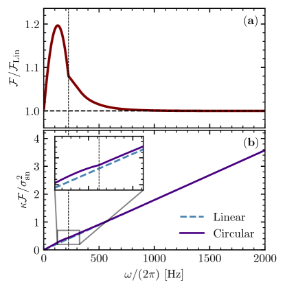
Figure 1: (a) Ratio of circular motion response function (I.8) to linear motion response function (S51). (b) Ratio of response to shot noise, for both circular motion and linear motion. The plots are at temperature $T=10\,\mathrm{mK}$.

Figure 1 compares the circular motion and linear motion response functions over our frequency range. As the two closely agree at high frequencies, a measurement of $\mathcal{F}(\omega;T)$ at high frequencies determines $\mathcal{F}_{\mathrm{Lin}}(\omega;T)$ over our full frequency range, by the linearity of (S51). A measurement of $\mathcal{F}(\omega;T)$ at lower frequencies, where $\mathcal{F}(\omega;T)$ and $\mathcal{F}_{\mathrm{Lin}}(\omega;T)$ differ, then determines $S_{\delta}(\omega)$ (13) at the lower frequencies.

References

- Unruh [1976] W. G. Unruh, Phys. Rev. D 14, 870 (1976).
- Bunney and Louko [2023] C. R. D. Bunney and J. Louko, (2023), arXiv:2303.12690 [gr-qc] .
- Gooding et al. [2020] C. Gooding, S. Biermann, S. Erne, J. Louko, W. G. Unruh, J. Schmiedmayer, and S. Weinfurtner, Phys. Rev. Lett. 125, 213603 (2020).
- Unruh [2022] W. G. Unruh, J. Low Temp. Phys. 208, 196 (2022).
- Weinfurtner et al. [2011] S. Weinfurtner, E. W. Tedford, M. C. J. Penrice, W. G. Unruh, and G. A. Lawrence, Phys. Rev. Lett. 106, 021302 (2011).
- Torres et al. [2017] T. Torres, S. Patrick, A. Coutant, M. Richartz, E. W. Tedford, and S. Weinfurtner, Nature Phys. 13, 833 (2017).
- Torres et al. [2020] T. Torres, S. Patrick, M. Richartz, and S. Weinfurtner, Phys. Rev. Lett. 125, 011301 (2020).
- Atkins [1959] K. R. Atkins, Phys. Rev. 113, 962 (1959).
- Schützhold and Unruh [2002] R. Schützhold and W. G. Unruh, Phys. Rev. D 66, 044019 (2002).
- McAuslan et al. [2016] D. L. McAuslan, G. I. Harris, C. Baker, Y. Sachkou, X. He, E. Sheridan, and W. P. Bowen, Phys. Rev. X 6, 021012 (2016).
- Harris et al. [2016] G. I. Harris, D. L. McAuslan, E. Sheridan, Y. Sachkou, C. Baker, and W. P. Bowen, Nature Phys. 12, 788 (2016).
- Childress et al. [2017] L. Childress, M. P. Schmidt, A. D. Kashkanova, C. D. Brown, G. I. Harris, A. Aiello, F. Marquardt, and J. G. E. Harris, Phys. Rev. A 96, 063842 (2017).
- Singh et al. [2017] S. Singh, L. A. De Lorenzo, I. Pikovski, and K. C. Schwab, New J. Phys. 19, 073023 (2017).
- Sachkou et al. [2019] Y. P. Sachkou, C. G. Baker, G. I. Harris, O. R. Stockdale, S. Forstner, M. T. Reeves, X. He, D. L. McAuslan, A. S. Bradley, M. J. Davis, et al., Science 366, 1480 (2019).
- Shkarin et al. [2019] A. B. Shkarin, A. D. Kashkanova, C. D. Brown, S. Garcia, K. Ott, J. Reichel, and J. G. E. Harris, Phys. Rev. Lett. 122, 153601 (2019).
- De Lorenzo and Schwab [2014] L. A. De Lorenzo and K. C. Schwab, New J. Phys. 16, 113020 (2014).
- De Lorenzo and Schwab [2017] L. A. De Lorenzo and K. C. Schwab, J. Low Temp. Phys. 186, 233 (2017).
- Kashkanova et al. [2017] A. D. Kashkanova, A. B. Shkarin, C. D. Brown, N. E. Flowers-Jacobs, L. Childress, S. W. Hoch, L. Hohmann, K. Ott, J. Reichel, and J. G. E. Harris, Nature Phys. 13, 74 (2017).
- Spence et al. [2021] S. Spence, Z. X. Koong, S. A. R. Horsley, and X. Rojas, Phys. Rev. Applied 15, 034090 (2021).
- Walls and Milburn [2008] D. F. Walls and G. J. Milburn, Quantum Optics (Springer, 2008).
- Stefszky et al. [2012] M. S. Stefszky, C. M. Mow-Lowry, S. S. Y. Chua, D. A. Shaddock, B. C. Buchler, H. Vahlbruch, A. Khalaidovski, R. Schnabel, P. K. Lam, and D. E. McClelland, Class. Quantum Grav. 29, 145015 (2012).
- Landau [1941] L. Landau, Phys. Rev. 60, 356 (1941).
- Donnelly and Barenghi [1998] R. J. Donnelly and C. F. Barenghi, J. Phys. Chem. Ref. Data 27, 1217 (1998).
- Mc McClintock et al. [1992] P. V. E. Mc McClintock, D. J. Meredith, and J. K. Wigmore, Liquid helium-4, in Low-Temperature Physics: an introduction for scientists and engineers (Springer Netherlands, Dordrecht, 1992) pp. 151–189.
- White [2006] I. White, Third Sound in Thin Film Superfluid 3He, Ph.D. thesis, University of Manchester (2006).
- Atkins and Rudnick [1970] K. R. Atkins and I. Rudnick, Prog. Low Temp. Phys. 6, 37 (1970).
- Rutledge et al. [1978] J. E. Rutledge, W. L. McMillan, J. M. Mochel, and T. E. Washburn, Phys. Rev. B 18, 2155 (1978).
- Baker et al. [2016] C. G. Baker, G. I. Harris, D. L. McAuslan, Y. Sachkou, X. He, and W. P. Bowen, New J. Phys. 18, 123025 (2016).
- Tilley and Tilley [1990] D. R. Tilley and J. Tilley, Superfluidity and Superconductivity (Adam Hilger, Bristol, 1990).
- Roche et al. [1995] P. Roche, G. Deville, K. O. Keshishev, N. J. Appleyard, and F. I. B. Williams, Phys. Rev. Lett. 75, 3316 (1995).
- Unruh [1981] W. G. Unruh, Phys. Rev. Lett. 46, 1351 (1981).
- Agarwal and Jha [2014] G. S. Agarwal and S. S. Jha, Phys. Rev. A 90, 023812 (2014).
- Bell and Leinaas [1983] J. S. Bell and J. M. Leinaas, Nucl. Phys. B 212, 131 (1983).
- Bell and Leinaas [1987] J. S. Bell and J. M. Leinaas, Nucl. Phys. B 284, 488 (1987).
- Unruh [1998] W. G. Unruh, Phys. Rept. 307, 163 (1998).
- Biermann et al. [2020] S. Biermann, S. Erne, C. Gooding, J. Louko, J. Schmiedmayer, W. G. Unruh, and S. Weinfurtner, Phys. Rev. D 102, 085006 (2020).
- Hoffmann et al. [2004] J. A. Hoffmann, K. Penanen, J. C. Davis, and R. E. Packard, J. Low Temp. Phys. 135, 177 (2004).
- Luke [1967] J. C. Luke, J. Fluid Mech. 27, 395 (1967).
- [39] DLMF, NIST Digital Library of Mathematical Functions, http://dlmf.nist.gov/, Release 1.1.8 of 2022-12-15, F. W. J. Olver, A. B. Olde Daalhuis, D. W. Lozier, B. I. Schneider, R. F. Boisvert, C. W. Clark, B. R. Miller, B. V. Saunders, H. S. Cohl, and M. A. McClain, eds.