DoG is SGD’s Best Friend:
A Parameter-Free Dynamic Step Size Schedule

Abstract

We propose a tuning-free dynamic SGD step size formula, which we call Distance over Gradients (DoG). The DoG step sizes depend on simple empirical quantities (distance from the initial point and norms of gradients) and have no “learning rate” parameter. Theoretically, we show that a slight variation of the DoG formula enjoys strong parameter-free convergence guarantees for stochastic convex optimization assuming only locally bounded stochastic gradients. Empirically, we consider a broad range of vision and language transfer learning tasks, and show that DoG’s performance is close to that of SGD with tuned learning rate. We also propose a per-layer variant of DoG that generally outperforms tuned SGD, approaching the performance of tuned Adam. A PyTorch implementation is available at https://github.com/formll/dog.

1 Introduction

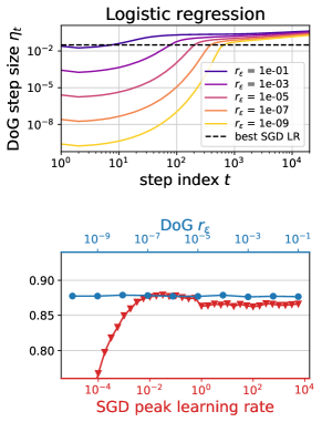
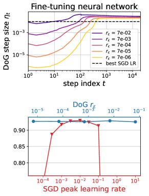
Figure 1: Illustration of DoG for CIFAR-100 classification using logistic regression on last-layer features of a pre-trained ViT-B/32 (left) or end-to-end fine-tuning of the model (right). The top row shows the DoG step size sequence $\eta_{t}$ for different values of the initial movement $r_{\epsilon}$, and the bottom row shows that DoG attains test error on par with carefully tuned SGD (with cosine annealing), even when varying $r_{\epsilon}$ by several orders of magnitude. See details in Section E.6.

While stochastic optimization methods drive continual improvements in machine learning, choosing the optimization parameters—and particularly the learning rate—remains a difficulty. Standard methodologies include searching over a set of learning rates, or simply picking the learning rate from prior work. The former incurs a substantial computational overhead, while the latter risks training a suboptimal model.

The rich literature on adaptive gradient methods (AdaGrad, Adam, and their many variants) offers optimization algorithms that better exploit problem structure [e.g., 29, 48, 34, 84, 57]. However, these methods still have a learning rate parameter that requires tuning. The theoretically-optimal value of this parameter depends on unknown problem properties. For example, on convex problems the optimal learning rate of AdaGrad is related to the distance between the initial point and the optimal solution, while in non-convex settings it is related to the function’s smoothness and initial optimality gap [33, 95, 30].

Parameter-free optimization aims to remove the need for such tuning by designing algorithms that achieve a near-optimal rate of convergence with almost no knowledge of the problem properties [87]. Most works in this field [e.g., 58, 69, 21, 61, 10, 42, 110] use advanced online learning techniques to construct algorithms that, for the fundamental setting of stochastic convex optimization (SCO) with bounded stochastic gradients, achieve optimal rates of convergence up to logarithmic factors. While practical parameter-free algorithms exist [e.g. 68, 71, 47, 15], there is little research into practical parameter-free step size selection methods for SGD. Recently, Carmon and Hinder [11] have shown that performing a careful bisection over the SGD step size yields a parameter-free optimization method that is optimal for SCO up to a double-logarithmic factor. While theoretically novel, on a practical level the result leaves much to be desired, as it essentially prescribes the standard recipe of running SGD multiple times with different learning rates.

Proposed algorithm.

In this work, we use key insights from Carmon and Hinder [11] to go a step further and develop a parameter-free step size schedule. For SGD iterations of the form $x_{t+1}=x_{t}-\eta_{t}g_{t}$, where $x_{t}$ denotes the model parameters at the $t$’th iteration and $g_{t}$ denotes the stochastic gradient of the loss function, our proposed steps size sequence is (for all $t\geq 1$)

$$\eta_{t}=\frac{\max_{i\leq t}\|x_{i}-x_{0}\|}{\sqrt{\sum_{i\leq t}\|g_{i}\|^{2}}}.$$ (DoG)

In words, the step size at iteration $t$ is the maximum distance to between the initial point and observed iterates, divided by the sum of squared stochastic gradient norms, i.e., Distance over Gradients (DoG). At the first step, we set $\eta_{0}$ to be $r_{\epsilon}/\|g_{0}\|$, i.e., we take a normalized gradient step of size $r_{\epsilon}$; we show that, as long as $r_{\epsilon}$ is small, its precise setting has only mild effect.

Crucially, DoG has no multiplicative “learning rate” parameter: if one considers step sizes of the form $\eta_{t}=c\cdot\frac{\max_{i\leq t}\|x_{i}-x_{0}\|}{\sqrt{\sum_{i\leq t}\|g_{i}\|^{2}}}$ then $c=1$ is a universally good setting (see Section 2 for a heuristic justification and Section 4.3 for empirical evidence for this claim).

Figure 1 highlights key aspects of DoG. The top row shows the DoG step size sequence for different values of $r_{\epsilon}$ in convex (left) and non-convex (right) stochastic optimization problems. The DoG step size increases rapidly (note the logarithmic $x$ scale) and stabilizes around values close to the optimal SGD step size with little dependence on $r_{\epsilon}$. The bottom row of the figure compares the test errors of DoG and SGD with various step sizes, showing that (for all choices of $r_{\epsilon}$) DoG is on par with well-tuned SGD.

1.1 Summary of results

Theoretical guarantees.

In Section 3 we analyze DoG for stochastic convex optimization with bounded stochastic gradients and a (potentially unbounded) closed convex domain. To present our results, let $\mathcal{B}$ denote a ball around the initial point $x_{0}$ with radius $3d_{0}$, where $d_{0}$ is the distance between $x_{0}$ and an optimum.

First, we show that if the iterates of DoG remain in $\mathcal{B}$, then with high probability DoG achieves a convergence rate that is optimal up to a factor of $O(\log(1+\frac{d_{0}}{r_{\epsilon}}))$. In practice, DoG appears to indeed be stable as long as $r_{\epsilon}$ is sufficiently small. However, DoG is not always stable: on pathological functions its iterates can move far from the optimum.

To address this, we consider a theoretical, tamed variant of DoG, which we call T-DoG, whose step sizes are smaller by a logarithmic factor. We prove that, with high probability, the T-DoG iterates never leave $\mathcal{B}$. Thus, we obtain a high probability parameter-free convergence guarantee that is optimal up logarithmic factors.

To our knowledge, this is the first dynamic SGD step size schedule to attain such theoretical guarantee, and only the third high probability parameter-free guarantee in the literature [following 11, 109]. Moreover, it is the first parameter-free result assuming only locally bounded stochastic gradients (i.e., in the set $\mathcal{B}$). This is significant since the usually-assumed global stochastic gradient bound does not exist in many problems, including least squares.

Empirical study.

Our experiments in Section 4 focus on fine-tuning neural networks, because this is a practically important setting that still allows for thorough experiments at a reasonable computational budget. We also perform a small-scale experiment with training a neural network from scratch. Our experiments span 23 natural language understanding and image classification tasks and 8 popular model architectures.

Our results indicate that, compared to DoG, SGD with a cosine step size schedule and tuned base learning rarely attains a relative error improvement of more than 5% (e.g., the difference between accuracy 95% and 95.25%). For convex problems (linear probes), the relative difference in errors is below 1%. In our testbed, well-tuned Adam tends to outperform both SGD and DoG, but a layer-wise version of DoG (which we call L-DoG) closes some of this performance gap.

We also test the sensitivity of DoG to the value of $r_{\epsilon}$. We find that for most model/task combinations, DoG performs consistently well across a wide range of $r_{\epsilon}$ values as our theory predicts. However, in certain cases, choosing $r_{\epsilon}$ to be too low results in poor performance. We provide some preliminary findings showing that this is due in part to batch normalization.

Put together, our theory and experiments suggest DoG has the potential to save significant computation currently spent on learning rate tuning at little or no cost in performance—especially if we reinvest some of the saved computation in training a larger model on more data.

2 Algorithm Derivation

Before providing rigorous theoretical guarantees for DoG, in this section we explain the origin of the algorithm. Our starting point is the following result by Carmon and Hinder [11]. Suppose we run $T$ iterations of SGD with fixed step size $\eta$, i.e., the recursion $x_{t+1}=x_{t}-\eta g_{t}$, where $x_{t}$ is the SGD iterate and $g_{t}$ is the stochastic gradient at step $t$. If, for some $c\in(0,1)$, it happens to hold that

$$\eta=c\cdot\frac{\max_{k\leq T}\|x_{k}-x_{0}\|}{\sqrt{\sum_{k\leq T}\|g_{k}\|^{2}}},$$ (1)

then the averaged iterates satisfies an excess loss bound that is at most a factor $\frac{1}{c(1-c^{2})}$ larger than the worst-case optimal bound achieved by perfectly tuned SGD.

The condition (1) is an implicit equation: it allows us to check whether the choice of step size $\eta$ is good only after running $T$ steps of SGD using that $\eta$. Solving this implicit equation therefore requires multiple calls to SGD. We derive the DoG step size sequence by making the equation explicit: we choose $\eta_{t}$ so that equation (1) holds at each step. For $c=1$, this yields the step size formula (DoG). Our reason for choosing $c=1$ is that it is the threshold under which a solution to the implicit equation yields an optimal rate of convergence. Therefore, in practice we expect $1$ to be close to the highest stable value of $c$, and thus obtain the best performance; we verify this empirically in Section 4.3.

3 Theoretical Analysis

3.1 Preliminaries

Problem setting.

Our goal is to minimize a loss function $f:\mathcal{X}\rightarrow\mathbb{R}$ where $\mathcal{X}\subseteq\mathbb{R}^{m}$ (including the unconstrained setting $\mathcal{X}=\mathbb{R}^{m}$ as an important special case). We perform our analysis under the following standard convexity assumption.

Assumption 1 (Convexity).

The function $f$ is convex, its domain $\mathcal{X}$ is closed and convex, and its minimum is attained at some $x_{\star}\in\mathcal{X}$, i.e., $f_{\star}\coloneqq\inf_{x\in\mathcal{X}}f(x)=f(x_{\star})$.

In Appendix A we discuss a possible relaxation of convexity under which our results continue to hold.

To minimize $f$ we assume access to a stochastic gradient oracle $\mathcal{G}$. When queried at a point $x\in\mathcal{X}$ the oracle returns a stochastic (sub)gradient estimator $\mathcal{G}(x)$ satisfying $\mathbb{E}[\mathcal{G}(x)\;|\;x]\in\partial f(x)$. With slight abuse of notation, we write $\nabla f(x)\coloneqq\mathbb{E}[\mathcal{G}(x)\mid x]$. We make the following assumption, where $\|\cdot\|$ denotes the Euclidean norm.

Assumption 2 (Pointwise bounded stochastic gradients).

There exists some continuous function $\ell:\mathcal{X}\rightarrow\mathbb{R}$ such that $\|\mathcal{G}(x)\|\leq\ell(x)$ almost surely.

Assumption 2, which appeared in prior work [20, 61], is weaker than conventional assumptions in parameter-free stochastic optimization, which either uniformly bound the stochastic gradients, i.e., $\|\mathcal{G}(x)\|\leq L$ for all $x\in\mathcal{X}$ [see, e.g., 71, 21], or uniformly bound the gradient variance [44]. However, even least squares problems (with $\mathcal{G}(x)=(\left<a,x\right>-b)a$ for random $a\in\mathbb{R}^{m}$ and $b\in\mathbb{R}$) violate both uniform bounds. In contrast, $\ell$ is finite under the mild assumption that $a,b$ are bounded random variables; see Section C.5 for additional discussion.

Algorithm statement.

We study (projected) SGD with dynamic learning rate schedule $\{\eta_{t}\}$, i.e.,

$$x_{t+1}=\mathbf{\mathrm{Proj}}_{\mathcal{X}}(x_{t}-\eta_{t}g_{t})$$

where $x_{0}$ is a given initialization, $g_{k}\coloneqq\mathcal{G}(x_{k})$, and $\mathbf{\mathrm{Proj}}_{\mathcal{X}}(\cdot)$ is the Euclidean projection onto $\mathcal{X}$. To succinctly state and analyze DoG, we define the following quantities:

$$r_{t}\coloneqq\|x_{t}-x_{0}\|~{}\mbox{,}~{}\bar{r}_{t}=\max_{k\leq t}r_{k}\vee r_{\epsilon}~{}\mbox{and}~{}G_{t}\coloneqq\sum_{k=0}^{t}\|g_{t}\|^{2},$$

where $a\vee b\coloneqq\max\{a,b\}$ and $r_{\epsilon}$ is a small user-specified initial movement size parameter. With this notation, we define a family of DoG-like learning rate schedules.

Definition 1.

A step size schedule is DoG-like if

$$\eta_{t}=\frac{\bar{r}_{t}}{\sqrt{G_{t}^{\prime}}}$$

for a positive nondecreasing sequence $G_{t}^{\prime}$ that depends only on $x_{0},g_{0},\ldots,g_{t}$ and satisfies $G_{t}^{\prime}\geq G_{t}$.

DoG corresponds to simply setting $G_{t}^{\prime}=G_{t}$; in Section 3.3 we consider a theoretical (or tamed) DoG-like algorithm for which we guarantee bounded iterates by making $G_{t}^{\prime}$ larger than $G_{t}$ by polylogarithmic factors. Throughout, we bound the error of the weighted average sequence

$$\bar{x}_{t}\coloneqq\frac{1}{\sum_{k=0}^{t-1}\bar{r}_{k}}\sum_{k=0}^{t-1}\bar{r}_{k}x_{k}.$$ (2)

Finally, to streamline the analysis we define:

$$d_{t}\coloneqq\|x_{t}-x_{\star}\|~{},~{}\bar{d}_{t}\coloneqq\max_{k\leq t}d_{k}~{}\mbox{,}~{}\bar{\ell}_{t}\coloneqq\max_{k\leq t}\ell(x_{k}),$$

and

$$\theta_{t,\delta}\coloneqq\log\left(\frac{60\log(6t)}{\delta}\right).$$

Logarithm conventions.

Throughout the paper $\log$ is base $e$ and $\log_{+}\left(\cdot\right)\coloneqq 1+\log(\cdot)$.

3.2 Optimality gap bounds assuming bounded iterates

In this section, we bound the optimality gap attained by any DoG-like algorithm. Our bounds depend on the quantities $\bar{r}_{T}$ and $G_{T}$, and are nearly optimal when $\bar{r}_{T}=O(d_{0})$ (i.e., the DoG iterates don’t move too far away from $x_{0}$) and $G_{T}^{\prime}$ is not much larger than $G_{T}$. In the next section we describe a specific DoG-like algorithm that is guaranteed to satisfy both requirements.

Convexity and Jensen’s inequality imply that $\bar{x}_{t}$ satisfies

$$f(\bar{x}_{t})-f_{\star}\leq\frac{1}{\sum_{k=0}^{t-1}\bar{r}_{k}}\sum_{k=0}^{t-1}\bar{r}_{k}\left<\nabla f(x_{k}),x_{k}-x_{\star}\right>.$$ (3)

The sum in the RHS decomposes to two components:

$$\underbrace{\sum_{k=0}^{t-1}\bar{r}_{k}\left<g_{k},x_{k}-x_{\star}\right>}_{\text{weighted regret}}-\underbrace{\sum_{k=0}^{t-1}\bar{r}_{k}\left<\Delta_{k},x_{k}-x_{\star}\right>}_{\text{noise}},$$ (4)

where $\Delta_{k}\coloneqq g_{k}-\nabla f(x_{k})$. We give probability 1 bounds for the weighted regret (Lemma 1) and high probability bounds for the noise term (Lemma 2). In each case, the key challenge is replacing a-priori bounds on $d_{0}$ (or the domain size) with the empirically observed $\bar{r}_{T}$. We present and discuss each lemma in turn.

Lemma 1 (Weighted regret bound).

If $\mathcal{X}$ is a closed convex set then any DoG-like scheme (Definition 1) satisfies $\sum_{k=0}^{t-1}\bar{r}_{k}\left<g_{k},x_{k}-x_{\star}\right>\leq\bar{r}_{t}(2\bar{d}_{t}+\bar{r}_{t})\sqrt{G_{t-1}^{\prime}}$, $\forall t\geq 1$.

Proof.

Using $x_{k+1}=\mathbf{\mathrm{Proj}}_{\mathcal{X}}(x_{k}-\eta_{k}g_{k})$ we obtain the standard inequality $d_{k+1}^{2}\leq\|x_{k}-\eta_{k}g_{k}-x_{\star}\|^{2}=d_{k}^{2}-2\eta_{k}\left<g_{k},x_{k}-x_{\star}\right>+\eta_{k}^{2}\|g_{k}\|^{2}$. Rearranging this gives:

$$\left<g_{k},x_{k}-x_{\star}\right>\leq\frac{d_{k}^{2}-d_{k+1}^{2}}{2\eta_{k}}+\frac{\eta_{k}\|g_{k}\|^{2}}{2}.$$ (5)

Therefore, $\sum_{k=0}^{t-1}\bar{r}_{k}\left<g_{k},x_{k}-x_{\star}\right>$ is at most

$$\frac{1}{2}\underbrace{\sum_{k=0}^{t-1}\frac{\bar{r}_{k}}{\eta_{k}}(d_{k}^{2}-d_{k+1}^{2})}_{(A)}+\frac{1}{2}\underbrace{\sum_{k=0}^{t-1}\bar{r}_{k}\eta_{k}\|g_{k}\|^{2}}_{(B)}.$$

We bound the terms $(A)$ and $(B)$ in turn, beginning with the former:

$$(A) =\sum_{k=0}^{t-1}\sqrt{G_{k}^{\prime}}(d_{k}^{2}-d_{k+1}^{2})=d_{0}^{2}\sqrt{G_{0}^{\prime}}-d_{t}^{2}\sqrt{G_{t-1}^{\prime}}+\sum_{k=1}^{t-1}d_{k}^{2}\left(\sqrt{G_{k}^{\prime}}-\sqrt{G_{k-1}^{\prime}}\right)$$

$$\overset{(i)}{\leq}\bar{d}_{t}^{2}\sqrt{G_{0}^{\prime}}-d_{t}^{2}\sqrt{G_{t-1}^{\prime}}+\bar{d}_{t}^{2}\sum_{k=1}^{t-1}\left(\sqrt{G_{k}^{\prime}}-\sqrt{G_{k-1}^{\prime}}\right)=\sqrt{G_{t-1}^{\prime}}\left(\bar{d}_{t}^{2}-d_{t}^{2}\right)\overset{(ii)}{\leq}4\bar{r}_{t}\bar{d}_{t}\sqrt{G_{t-1}^{\prime}}.$$

Inequality $(i)$ uses $d_{k}\leq\bar{d}_{t}$ and that $G_{k}^{\prime}$ is nondecreasing as per Definition 1. Inequality $(ii)$ holds since, for $s\in\operatorname*{arg\,max}_{k\leq t}d_{k}$, we have $\bar{d}_{t}^{2}-d_{t}^{2}=d_{s}^{2}-d_{t}^{2}=(d_{s}-d_{t})(d_{s}+d_{t})\leq\|x_{s}-x_{t}\|(d_{s}+d_{t})\leq(\bar{r}_{s}+\bar{r}_{t})(d_{s}+d_{t})\leq 4\bar{r}_{t}\bar{d}_{t}$. Bounding the second term $(B)$, we have:

$$(B) =\sum_{k=0}^{t-1}\frac{\bar{r}_{k}^{2}\|g_{k}\|^{2}}{\sqrt{G_{k}^{\prime}}}\leq\sum_{k=0}^{t-1}\frac{\bar{r}_{k}^{2}\|g_{k}\|^{2}}{\sqrt{G_{k}}}\leq\bar{r}_{t}^{2}\sum_{k=0}^{t-1}\frac{\|g_{k}\|^{2}}{\sqrt{G_{k}}}\leq 2\bar{r}_{t}^{2}\sqrt{G_{t-1}},$$

where the final inequality uses the standard Lemma 4 with $a_{k}=G_{k}=\sum_{i\leq k}\|g_{i}\|^{2}$. ∎

While the proof of Lemma 1 is similar to the analysis of adaptive SGD where $\eta_{t}=\frac{\rho}{\sqrt{G_{t}}}$ [33], there are a couple of key differences. First, the DoG step sizes can increase, which typically makes adaptive gradient methods difficult to analyze [80]. We bypass this difficulty by considering regret weighted by $\bar{r}_{k}$, which factors out the increasing portion of the step size. Second, the standard adaptive SGD analysis yields a bound proportional to $\bar{d}_{t}^{2}$ (typically further bounded using the domain diameter) rather than $\bar{r}_{t}\bar{d}_{t}$ as in our bound. This is a crucial difference, since—as we soon argue—$\bar{r}_{t}$ “cancels” when dividing through by $\sum_{k<t}\bar{r}_{k}$, while $\bar{d}_{t}$ does not. We obtain the improved result by keeping around the term $-d_{t}^{2}\sqrt{G_{t-1}^{\prime}}$ in the bound for $(A)$ above; a trick similar to Carmon and Hinder [11, Lemma 1].

Next, we handle the noise term in (4), recalling the notation $\Delta_{t}\coloneqq g_{t}-\nabla f(x_{t})$ and $\theta_{t,\delta}\coloneqq\log\frac{60\log(6t)}{\delta}$.

Lemma 2 (Noise bound).

Under Assumption 2, for all $\delta\in(0,1)$, $T\in\mathbb{N}$ and $L>0$ we have

$$\mathbb{P}\left(\exists t\leq T:\Bigg{\lvert}\sum_{k=0}^{t-1}\bar{r}_{k}\left<\Delta_{k},x_{k}-x_{\star}\right>\Bigg{\rvert}\geq 8\bar{r}_{t-1}\bar{d}_{t-1}\sqrt{\theta_{t,\delta}G_{t-1}+\theta_{t,\delta}^{2}L^{2}}\right)\leq\delta+\mathbb{P}\left(\bar{\ell}_{T}>L\right).$$

The proof of Lemma 2 appears in Appendix C.1 and is based on a new concentration bound, Lemma 7, which allows us to bound the noise term despite having no deterministic bound on the magnitude of the martingale difference sequence $\bar{r}_{k}\left<\Delta_{k},x_{k}-x_{\star}\right>$. The proof of Lemma 7 involves combining time-uniform Bernstein bounds [39] and a general bound on the cumulative sums of sequence products (Lemma 5), which may be of independent interest.

Combining the above results, we obtain the following.

Proposition 1.

For all $\delta\in(0,1)$ and $L>0$, if Assumption 1, Assumption 2, and Definition 1 hold then with probability at least $1-\delta-\mathbb{P}\left(\bar{\ell}_{T}>L\right)$, for all $t\leq T$ the optimality gap $f(\bar{x}_{t})-f_{\star}$ is

$$O\left(\frac{(d_{0}+\bar{r}_{t})\sqrt{G_{t-1}^{\prime}+G_{t-1}\theta_{t,\delta}+L^{2}\theta_{t,\delta}^{2}}}{\sum_{i<t}\bar{r}_{i}/\bar{r}_{t}}\right).$$

Proof.

Follows from Equations 3 and 4, Lemma 1, Lemma 2 and the fact that $\bar{d}_{t}\leq d_{0}+\bar{r}_{t}$. ∎

The following algebraic fact shows that there is always an iteration $\tau\leq T$ where the denominator $\sum_{i<t}\frac{\bar{r}_{i}}{\bar{r}_{t}}\geq\Omega(T/\log\frac{\bar{r}_{T}}{r_{\epsilon}})$; see Section B.1 for proof.

Lemma 3.

Let $s_{0},s_{1},\ldots,s_{T}$ be a positive nondecreasing sequence. Then

$$\max_{t\leq T}\sum_{i<t}\frac{s_{i}}{s_{t}}\geq\frac{1}{e}\left(\frac{T}{\log_{+}(s_{T}/s_{0})}-1\right).$$

Combining Proposition 1 and Lemma 3 yields the following (see short proof in Section C.2).

Corollary 1.

Under Assumptions 1 and 2, for any $D\geq d_{0}$, let $L_{D}\coloneqq\max_{x\in\mathcal{X}:\|x-x_{0}\|\leq D}\ell(x)$. Then, for all $\delta\in(0,1)$ and for $\tau\in\operatorname*{arg\,max}_{t\leq T}\sum_{i<\tau}\frac{\bar{r}_{i}}{\bar{r}_{t}}$, with probability at least $1-\delta-\mathbb{P}(\bar{r}_{T}>D)$, the DoG iterates satisfy the optimality gap bound

$$f(\bar{x}_{\tau})-f_{\star}=O\left(\frac{D\sqrt{G_{\tau-1}\theta_{\tau,\delta}+L_{D}^{2}\theta_{\tau,\delta}^{2}}}{T}\log_{+}\left(\frac{D}{r_{\epsilon}}\right)\right)=O\left(\frac{DL_{D}}{\sqrt{T}}\theta_{\tau,\delta}\log_{+}\left(\frac{D}{r_{\epsilon}}\right)\right).$$

Corollary 1 is immediately useful when $\mathcal{X}$ is bounded but its exact diameter is unknown, for example when $\mathcal{X}$ is a polytope as is common in two-stage stochastic programming [64].

Simplifying the bound for typical DoG trajectories.

Suppose that the DoG iterates satisfy $\bar{r}_{T}\leq 3d_{0}$, which implies that $\bar{\ell}_{T}\leq L_{\star}\coloneqq L_{3d_{0}}$ and therefore (for DoG) $G_{t}^{\prime}=G_{t}\leq L_{\star}^{2}T$. Substituting into Corollary 1 yields an optimality gap bound of $O\left(\frac{d_{0}L_{\star}}{\sqrt{T}}\theta_{T,\delta}\log\frac{\bar{r}_{T}}{r_{\epsilon}}\right)$, which is minimax optimal up to a term double-logarithmic in $T$ and logarithmic in $\frac{1}{r_{\epsilon}}$ [2].

Furthermore, in realistic DoG trajectories, even the multiplicative term $\log\frac{\bar{r}_{T}}{r_{\epsilon}}$ is likely too pessimistic. This is because $\bar{r}_{t}$ typically increases rapidly for $t_{0}<1000$ steps and then plateaus (see Figure 12 in the appendix). Consequently, $\bar{r}_{i}/\bar{r}_{t}\geq 1/10$ for most of the optimization trajectory, and $\sum_{i<t}\frac{\bar{r}_{i}}{\bar{r}_{t}}\geq t/10-t_{0}$. Substituting back into Proposition 2, we get that $\bar{x}_{T}$ is $O\left(\frac{d_{0}L_{\star}}{\sqrt{T-t_{0}}}\theta_{T,\delta}\right)$ suboptimal.

DoG can run wild.

While DoG is empirically stable, there exist (non-stochastic) examples where $\bar{r}_{t}$ grows much larger than $d_{0}$: in Appendix C.3 we describe a variant of Nemirovski’s function [63, 62] for which $\bar{r}_{t}=r_{\epsilon}\sqrt{t}$ and therefore $\bar{r}_{t}/d_{0}$ diverges as $t$ grows. Next, we show that by slightly decreasing the DoG step sizes we can guarantee that $\bar{r}_{T}/d_{0}\leq 3$ with high probability.

3.3 Iterate stability bound

This section introduces a new DoG-like step size scheme whose iterates are guaranteed to remain bounded with high probability. We call this scheme T-DoG, where the T stands for “theoretical” or “tamed.” The step sizes are given by $\eta_{t}={\bar{r}_{t}}/{\sqrt{G_{t}^{\prime}}}$, where

$$G_{t}^{\prime}=8^{4}\theta_{T,\delta}^{2}\log_{+}^{2}\left(1+\frac{t\bar{\ell}_{t}^{2}}{\bar{\ell}_{0}^{2}}\right)(G_{t-1}+16\bar{\ell}_{t}^{2}),$$ (T-DoG)

using $G_{-1}\coloneqq 0$, and recalling that $\bar{\ell}_{t}\coloneqq\max_{i\leq t}\ell(x)$ for a function $\ell$ satisfying Assumption 2. The T-DoG formula depends weakly on the iteration budget $T$ and the failure probability $\delta$ via $\theta_{t,\delta}\coloneqq\log\left(\frac{\log(6t)}{\delta}\right)$; as we show below, in the non-stochastic setting we may simply replace $\theta_{t,\delta}$ with 1. Moreover, the term $16\bar{\ell}_{t}$ typically grows slowly with $t$, becoming negligible compared to $G_{t-1}$. Notably, the T-DoG step size requires no global upper bound on stochastic gradient norms.

We are ready to state T-DoG’s key property: guaranteed iterate stability.

Proposition 2.

Suppose that Assumptions 1 and 2 hold and $r_{\epsilon}\leq 3d_{0}$. For any $\delta\in(0,1)$, and $T\in\mathbb{N}$, the iterations of T-DoG satisfy $\mathbb{P}\left(\bar{r}_{T}>3d_{0}\right)\leq\delta$.

We defer the full proof to Section C.4 and proceed to highlight the key argument by proving the result in the noiseless case.

Proof of Proposition 2 in the noiseless case.

In the noiseless case we have $g_{k}=\nabla f(x_{k})$ and therefore $\left<g_{k},x_{k}-x_{\star}\right>\geq f(x_{k})-f_{\star}\geq 0$. Substituting into (5) and rearranging gives $d_{k+1}^{2}-d_{k}^{2}\leq\eta_{k}^{2}\|g_{k}\|^{2}$. Assuming by induction that $\bar{r}_{t}\leq 3d_{0}$ and telescoping yields $d_{k+1}^{2}-d_{k}^{2}\leq\eta_{k}^{2}\|g_{k}\|^{2}$. Assuming by induction that $\bar{r}_{t}\leq 3d_{0}$ and telescoping yields

$$d_{t+1}^{2}-d_{0}^{2} \leq\bar{r}_{t}^{2}\sum_{k=0}^{t}\frac{\|g_{k}\|^{2}}{G_{k}^{\prime}}\overset{(i)}{\leq}\frac{\bar{r}_{t}^{2}}{8^{4}}\sum_{k=0}^{t}\frac{G_{k}-G_{k-1}}{(G_{k}+\bar{\ell}_{k}^{2})\log_{+}^{2}\frac{G_{k}+\bar{\ell}_{k}^{2}}{\bar{\ell}_{0}^{2}}}\overset{(ii)}{\leq}\frac{\bar{r}_{t}^{2}}{8^{4}}\overset{(iii)}{\leq}\frac{9d_{0}^{2}}{8^{4}}\implies d_{t+1}\leq 2d_{0},$$

where $(i)$ uses that $\|g_{k}\|^{2}=G_{k}-G_{k-1}$ (with the shorthand $G_{-1}\coloneqq 0$) and

$$G_{k}^{\prime}\geq 8^{4}(G_{k-1}+\|g_{k}\|^{2}+\bar{\ell}_{k}^{2})\log_{+}^{2}\left(\frac{\sum_{i\leq t}\bar{\ell}_{t}^{2}}{\bar{\ell}_{0}^{2}}\right)\geq 8^{4}(G_{k}+\bar{\ell}_{k}^{2})\log_{+}^{2}\frac{G_{k}+\bar{\ell}_{k}^{2}}{\bar{\ell}_{0}^{2}}$$

by Assumption 2 which implies $\|g_{k}\|\leq\bar{\ell}_{k}$ for all $k$, $(ii)$ uses Lemma 6 with $a_{k}=G_{k}+\bar{\ell}_{k}^{2}$, and $(iii)$ uses the inductive assumption $\bar{r}_{t}\leq 3d_{0}$. Therefore, $r_{t+1}\leq d_{t+1}+d_{0}\leq 3d_{0}$ by the triangle inequality, completing the induction step. Note that this proof ignored the $\theta_{t,\delta}$ term in (T-DoG), demonstrating it is not necessary in the noiseless case. ∎

Given Assumption 2 we define

$$L_{\star}=\max_{x\in\mathcal{X}:\|x-x_{0}\|\leq 3\|x_{0}-x_{\star}\|}\ell(x).$$ (6)

With all the ingredients in hand, we state the main guarantee for T-DoG.

Theorem 1.

Suppose that Assumptions 1 and 2 hold. For any $\delta\in(0,\frac{1}{2})$, $T\in\mathbb{N}$, consider $T$ iterations of T-DoG with $r_{\epsilon}\leq 3d_{0}$. Then for $\tau\in\operatorname*{arg\,max}_{t\leq T}\sum_{i<\tau}\bar{r}_{i}/\bar{r}_{t}$ we have, with probability at least $1-2\delta$, that

$$f(\bar{x}_{\tau})-f_{\star}=O\left(c_{\delta,r_{\epsilon},T}\frac{d_{0}\sqrt{G_{\tau-1}+L_{\star}^{2}}}{T}\right)=O\left(c_{\delta,r_{\epsilon},T}\frac{d_{0}L_{\star}}{\sqrt{T}}\right),$$

where $c_{\delta,r_{\epsilon},T}=\log_{+}\left(T\frac{d_{0}L_{\star}}{f(x_{0})-f_{\star}}\right)\log_{+}\left(\frac{d_{0}}{r_{\epsilon}}\right)\log\left(\frac{\log_{+}(T)}{\delta}\right)$.

Proof.

The theorem follows from Corollary 1, Proposition 2 and the definition of T-DoG, where we note that Assumption 2 and convexity of $f$ imply $\bar{\ell}_{0}\geq\|\nabla f(x_{0})\|\geq(f(x_{0})-f(x_{\star}))/d_{0}$, while $\bar{r}_{T}\leq 3d_{0}$ gives $\bar{\ell}_{T}\leq L_{\star}$. Therefore, $\log_{+}\left(1+\frac{T\bar{\ell}_{T}^{2}}{\bar{\ell}_{0}^{2}}\right)=O\left(\log_{+}\left(T\frac{d_{0}L_{\star}}{f(x_{0})-f_{\star}}\right)\right)$. ∎

Theorem 1 yields the optimal convergence bound [2] up to logarithmic factors. To the best of our knowledge this is the first parameter-free stochastic optimization method that does not require the stochastic gradients to be uniformly bounded across the domain $\mathcal{X}$ and instead produces a bound that depends on the ‘local’ gradient bound $L_{\star}$. Crucially, the T-DoG step size formula does not require advance knowledge of $L_{\star}$.

Extension to unweighted iterate averaging.

While the weighted iterate average (2) is convenient to our analysis, bounds similar to Proposition 1, Corollary 1 and Theorem 1 hold also for the standard unweighted iterate average $\hat{x}_{T}=\frac{1}{T}\sum_{t=0}^{T-1}x_{t}$. For $\hat{x}_{T}$ it is also straightforward to show a $1/T$ error bound for DoG in the smooth noiseless case. See Appendix D for details.

4 Experiments

To test DoG in practical scenarios, we perform extensive experiments over a diverse set of tasks and model architectures in both the vision and language domains. We construct a testbed that consists of over 20 tasks and 7 model architecture, covering natural language understanding and computer vision (Section 4.1). In this testbed we compare DoG to SGD and Adam (Section 4.2), showing that DoG performs on par with tuned SGD, but not as well as tuned Adam. Nevertheless, a per-layer version of DoG (defined below) closes much of this gap with Adam without requiring tuning. We also use our testbed to analyze the sensitivity of DoG to its fixed parameters (Section 4.3), and demonstrate its effectiveness in convex logistic regression settings (Section 4.4). Finally, we apply DoG and L-DoG to fine-tuning a CLIP model on ImageNet (Section 4.5) and training a CIFAR10 model from scratch (Section 4.6), and provide preliminary comparison to previously-proposed tuning free methods (Section 4.7). A PyTorch implementation of DoG is available at https://github.com/formll/dog.

Layer-wise DoG.

Neural models in general and transformer-based models in particular often benefit from using a per-parameter or per-layer step sizes [48, 106]. With this in mind, we consider a per-layer version of DoG, which we call L-DoG, where we apply the (DoG) formula separately for every layer. Namely, if we consider $x_{t}^{l}$ to be the weights in layer $l$ at step $t$, then we set the learning rate for that layer to be $\eta_{t}^{l}=\frac{\max_{i\leq t}\|x_{i}^{l}-x_{0}^{l}\|}{\sqrt{\sum_{i\leq t}\|g_{i}^{l}\|^{2}+\epsilon}}$, where $\epsilon=10^{-8}$ is added to the denominator for numerical stability. While we do not provide theoretical guarantees for L-DoG, we show below that it performs well in practice.

4.1 Fine-tuning testbed

Our main experiments focus on fine-tuning pre-trained models, which allows us to experiment with advanced models while also thoroughly tuning the learning rate for the baseline optimizers, using an academic computational budget.

Common hyperparameters.

For each baseline algorithm, we use best-practice learning rate schedule (cosine annealing for all experiments, with a warmup stage for language experiments) and sweep over the peak learning rate for each model/task pair. We give each pair a fixed step budget designed to suffice for convergence, performing evaluation throughout the training. In all cases, we use polynomial decay averaging as proposed by Shamir and Zhang [83], and select the best checkpoint (either averaged or not) based on evaluation performance. We repeat relevant learning setups with 5 different seeds, and report the mean performance across the seeds. For simplicity, we do not use weight decay throughout. The complete set of hyper-parameters appears in Appendix E.

Natural language understanding (NLU).

To test DoG’s efficacy in modern NLU, we use it to fine-tune transformer language models [89] on the well-studied GLUE benchmark [94] which measures models’ performance on diverse text classification tasks (listed in Section E.3).

Additionally, we fine-tune models on SQuAD 1.1, a question answering dataset [79]. We fine-tune a RoBERTa-base [54] checkpoint and T5-base [78]. For each task, we use the official evaluation metrics defined in Wang et al. [94] and Rajpurkar et al. [79] as well as their original proposed splits, and report the results over the evaluation set.

Computer vision.

We also fine-tune 5 models architectures on 12 different computer vision tasks from the VTAB benchmark [108] (see Section E.3); of the other 7 tasks in VTAB, 5 are trivial (accuracy greater than 99%) and 2 have small validation splits leading to unreliable model selection. We follow the training, validation and test splits defined in VTAB, and report performance on the test split (using the validation split for model selection). We fine-tune 5 models: VGG11 [85], ResNet50 [37], Densenet121 [40], ViT-B/32 [28], and ConvNeXt-T [55], where the ViT model is pre-trained on ImageNet 21K and the others are trained on ImageNet 1K [26].

Normalized performance metric.

Since the performance metrics in our testbed vary substantially across tasks and models, they are challenging to compare in aggregate. To address this, we consider the following notion of relative error difference (RED), that provides a normalized performance difference measure. In particular, given a task and a model architecture, let $\mathrm{err}_{x}$ be the error of the model when trained with optimizer $x$ (Adam or SGD with a certain learning rate, or L-DoG) and let $\mathrm{err}_{\textsc{DoG}}$ be the error when trained with DoG. Then

$$\text{RED}(\mathrm{err}_{x},\mathrm{err}_{\textsc{DoG}})\coloneqq\frac{\mathrm{err}_{\textsc{DoG}}-\mathrm{err}_{x}}{\mathrm{err}_{\textsc{DoG}}}.$$

A positive RED value indicates that optimizer $x$ is better than DoG, and a negative value indicates the opposite. When the absolute value of RED is beneath a few percentage points, the compared methods are nearly equivalent. For example, a 5% RED is equivalent to the difference between accuracy 95% and 95.25%.

Setting $r_{\epsilon}$.

Our theoretical analysis suggests that the particular choice of $r_{\epsilon}$ does not matter as long as it is sufficiently small relative to the distance between the weight initialization $x_{0}$ and the optimum. Consequently, for vision experiments we set $r_{\epsilon}=\alpha\cdot(1+\|x_{0}\|)$ for $\alpha=10^{-4}$, assuming that the distance to the optimum is more than 0.01% of the initialization norm. For language experiments, this assumption turned out to be wrong (causing DoG to diverge in some cases), and we decreased $\alpha$ to $10^{-6}$ for DoG and to $10^{-8}$ for L-DoG, where the additive $10^{-6}$ term was too large in some layers. We believe that $10^{-6}$ and $10^{-8}$ should be good defaults for DoG and L-DoG, respectively, though networks with batch normalization or different initialization schemes could require a larger value; see Section 4.3 for additional discussion.

4.2 Comparison of fine-tuning performance

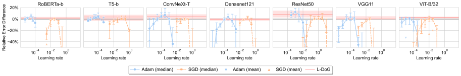
Figure 2: Relative error difference statistics (median, mean, and error bars showing IQR) across tasks for each model, as a function of peak learning rate. The red horizontal line and shaded region indicate the median and IQR RED for L-DoG, respectively.

Figure 2 depicts the median, IQR (inter-quantile range) and mean RED of each model, when trained with SGD and Adam with different peak learning rates. The figure shows that, when comparing across models, there is no good default learning rate for neither SGD nor Adam. Moreover, even for a single model only very specific SGD learning rate performs well, while most are considerably inferior to using DoG. Even when tuned to the best fixed learning-rate value per model (which we refer to as model tuned LR), some tasks may still fail (compared to DoG) as indicated by the large IQR and the gap between the mean (triangles) and the median RED (circles) in models such as ViT-B/32 ad Densenet121. While Adam also requires tuning, it is somewhat less sensitive than SGD to the choice of peak learning rate. For a full breakdown of performance per task, see Figure 7 and Sections F.1 and F.1 in Section F.1.

DoG performs similarly to well-tuned SGD in 79 out of the 80 model/task combinations in our testbed. The one exception is tuning T5-b on CoLA, where DoG behaves erratically while SGD succeeds only with a few learning rates. In contrast, both Adam and L-DoG achieved reasonable performance consistently. DoG’s poor performance on CoLA results in high RED measures for this case, which draw the mean RED (triangles) above the median one in Figure 2 for T5-b. We further analyze this exception in Section F.3 and show that choosing significantly smaller $r_{\epsilon}$ for DoG alleviates the problem.

Figure 3 (top) compares DoG to SGD with model tuned LR as defined above, as well as instance tuned LR, where for each model/task pair we select the best learning rate, at a computational expense 5–7 times larger than running DoG. The performance of DoG remains close to that of SGD with instance-tuned LR, with the largest median RED observed for ResNet50 and ViT-B/32.

Figure 3 (bottom) compares DoG to model-tuned and instance-tuned Adam, as well as to L-DoG. In a few cases (namely ResNet50 and ConvNeXt-T) the gaps between DoG and Adam are significant, and favor Adam. We hypothesize this is due to Adam’s per-parameter step-sizes and momentum mechanisms, which DoG does not exploit. L-DoG, which has per-layer steps, has positive median RED for all models, and narrows the gap between DoG and Adam, particularly for ResNet50.

The instance-tuned baselines consume significantly more compute than DoG and L-DoG. In Section F.2 we equalize the compute budget by reducing the number of steps for SGD and Adam. This makes DoG outperform instance-tune SGD in most cases, and brings L-DoG substantially closer to Adam.

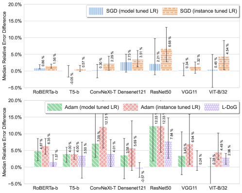
Figure 3: RED median (bar chart) and IQR (error bars) of each model on the set of applicable tasks. Top: Comparison with SGD when the LR is optimally tuned per model (model tuned LR) or per task (instance tuned LR). DoG is competitive with model-tuned SGD and often performs nearly as well as instance-tuned SGD. Bottom: Comparison of DoG with adaptive optimizers. L-DoG closes most of the gap to Adam.

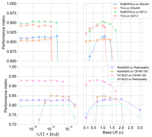
Figure 4: Performance metrics of models trained with DoG as a function of $\eta_{0}$ (left) or the base learning rate (right).

4.3 Sensitivity of DoG’s fixed parameters

Initial movement size $r_{\epsilon}$.

Our theory suggests that all sufficiently small choices of $r_{\epsilon}$ should perform similarly, but choosing $r_{\epsilon}$ too large (compared to the initial distance to the optimum) can hurt the performance of the algorithm. In Figure 4 (left) we plot the test performance as a function of $r_{\epsilon}$ for 8 model/task combinations. For 7 out of the 8, DoG is highly robust to the value of $r_{\epsilon}$ as long as it small enough, as predicted. However, ResNet50 on CIFAR-100 (bottom left) is an exception, where smaller values of $r_{\epsilon}$ result in an accuracy drop. We hypothesize this is due to scale invariance introduced by batch normalization (BN), and provide supporting evidence for that in Section F.4 (Figure 10), where we show that DoG is insensitive to $r_{\epsilon}$ when we turn off BN. In the appendix we also provide a complementary diagnostic for $r_{\epsilon}$ sensitivity by plotting $\eta_{t}$ vs. $\eta_{0}$ for different values of $t$ (see Figure 8).

Base learning rate.

For this experiment only, we consider variants of DoG with different values of base learning, i.e., step sizes of the form $\eta_{t}=c\cdot\frac{\max_{i\leq t}\|x_{i}-x_{0}\|}{\sqrt{\sum_{i\leq t}\|g_{i}\|^{2}}}$ with different values of $c$. We expect optimal performance when $c$ is close to 1. More specifically, we expect the algorithm to be unstable when $c>1$ and to be slower to converge (and less likely to generalize well) when $c<1$. As can be observed in Figure 4 (right), values around $c=1$ perform well for all models. For smaller values, there is indeed inferior performance in some models (mainly ResNet50 and RoBERTa-b)—indicating T-DoG would not work well in practice—while larger values result in divergence (in 6 out of 8 cases). Hence, the useful range for $c$ is very narrow (about [0.5, 1.5]) and tuning it is not likely to produce significant improvements. This is in contrast to Adam and SGD which generally require searching over a space spanning a few orders of magnitude to properly train a model.

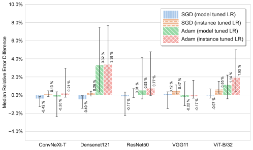
Figure 5: RED median and IQR (as in Figure 3) in tn the convex optimization setting (Section 4.4).

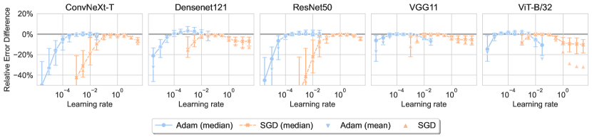
Figure 6: Per-learning rate RED statistics (as in Figure 2) in the convex optimization setting (Section 4.4).

4.4 Convex optimization

We also evaluate DoG on convex optimization tasks, matching the assumptions of our theoretical analysis. To do so, we perform multi-class logistic regression on features obtained from the computer vision models in our testbed, i.e., linear probes. We find that model-tuned SGD performs on par or worse than DoG, while instance-tuned SGD barely gains any advantage (Figure 5), with RED values well under 1% (corresponding to the difference between accuracies 90% and 90.1%). Moreover, even in this simple setting, SGD is sensitive to the choice of learning rate, which differ significantly between models (Figure 6).

Algorithm	LR	Acc. w/o averaging	Acc. with averaging
SGD	1e-03	60.70%	60.49%
	3e-03	73.62%	73.54%
	1e-02	76.82%	76.80%
	3e-02	77.51%	77.54%
	1e-01	75.73%	75.71%
DoG	-	74.78%	77.22%
AdamW	1e-05	78.23%	78.25%
	3e-05	79.04%	79.01%
	1e-04	75.02%	74.97%
L-DoG	-	78.20%	80.12%

Table 1: ImageNet top-1 validation accuracies after fine-tuning a CLIP ViT-B/32 model for 25K training steps, with and without polynomial decay averaging (see Section 4.5).

4.5 Fine-tuning on ImageNet

To complement our main fine-tuning testbed, we perform a more limited experiment involving ImageNet as a downstream task, which is more expensive to tune due its larger scale. We fine-tune a ViT-B/32 CLIP model [77] and compare DoG and L-DoG to training with SGD or AdamW [57]. We use a training prescription similar to Wortsman et al. [101]; see Section E.7 for additional details. Table 1 shows the ImageNet top-1 validation accuracies of the final model checkpoints, with and without the polynomial decay averaging used throughout our experiments. DoG performs similarly to SGD, but both algorithms perform significantly worse than AdamW, perhaps due to an insufficient iteration budget. L-DoG performs well in this setting, improving on AdamW by a little over 1 point.

Algorithm	LR	Acc. w/o averaging	Acc. with averaging
SGD	0.1	94.9%	94.9%
	0.3	95.8%	95.6%
	1	96.4%	84.4%
	3	95.9%	21.7%
	10	10.0%	10.0%
SGD w/ mom. 0.9	0.01	95.0%	95.1%
	0.03	95.8%	95.7%
	0.1 $\dagger$	96.3%	88.5%
	0.3	95.8%	27.5%
	1	42.0%	63.4%
DoG	-	85.2%	96.4%
Adam	3e-05	91.1%	91.1%
	1e-04	94.0%	94.0%
	3e-04	93.5%	93.8%
	1e-03	91.4%	91.6%
L-DoG	-	83.2%	93.5%

Table 2: CIFAR-10 test accuracies after training a Wide ResNet 28-10 model from scratch for 200 epochs, with and without polynomial decay averaging (see Section 4.6). $\dagger$ denotes the standard training configuration [cf. 19, Table 2].

4.6 Training from scratch

We conduct a preliminary experiment with training a model from scratch, specifically a Wide ResNet 28-10 [107] on CIFAR-10 [50]; see Section E.8 for details. Table 2 shows the test accuracy of the final checkpoint, with and without the polynomial averaging used throughout our experiments. Here DoG performs on par with the setting’s canonical training prescription of SGD with momentum 0.9 and learning rate 0.1 [19]. In this setting Adam produces poorer results, and L-DoG is 0.5 point worse than tuned Adam with the best learning rate, perhaps due to not reaching convergence.

4.7 Comparison to other tuning-free methods

We perform preliminary comparisons between DoG and L-DoG and other methods for removing the learning rate parameter: the Stochastic Polyak Step [56], D-Adaptation [24] and Continuous Coin Betting (COCOB) [71]. In all cases, we find that DoG and L-DoG provide better performance on most tasks and on average (see Sections G.4 and G.4). We provide detailed results in Appendix G, where we also discuss the practical prospects of the bisection procedure of Carmon and Hinder [11].

5 Related Work

Previous attempts to design theoretically principled and practical optimization algorithms that do not require learning rate tuning approach the problem from a variety of perspectives, resulting in a large variety of proposed algorithms. Rolinek and Martius [81], Vaswani et al. [90], Paquette and Scheinberg [72] lift classical line search technique from non-stochastic optimization to the stochastic setting, while Berrada et al. [9], Loizou et al. [56] do the same for the classical Polyak step size [76, 36]. Asi and Duchi [4] develop a class of algorithms based on stochastic proximal methods and demonstrate their improved robustness both theoretically and empirically. Schaul et al. [82] use a stochastic quadratic approximation for designing learning rates that maximize the expected one-step objective decrease. Chandra et al. [14] nest hypergradient descent to make a method that is insensitive to initial hyper-parameter choices. However, none of these results are parameter-free in the same sense as DoG: they either do not have converges guarantees, or have suboptimality bounds that blow up polynomially when the method’s parameters do not match a problem-dependent value. In contrast, parameter-free methods have convergence rates that depend at most logarithmically on algorithmic parameters.

While the parameter-free optimization literature has focused mainly on theoretical schemes, a number of works also include empirical studies [68, 71, 47, 15]. In particular, Orabona and Tommasi [71] build on coin-betting schemes to design an algorithm for training neural networks that has AdaGrad-style convergence guarantees for quasi-convex functions, showing promising results on neural network training problems. In recent work Chen et al. [15] obtain improved empirical results with an algorithm that leverages coin betting and truncated linear models. However, this method lacks theoretical guarantees.

In recent independent work Defazio and Mishchenko [24] propose a parameter-free dynamic step size schedule of dual averaging. While our work has the same motivation and shares a number of technical similarities (including the use of weighted regret bounds and an independently obtained Lemma 3), the proposed algorithms are quite different, and dual averaging is rarely used in training neural networks. (See additional discussion in Section G.3). Moreover, Defazio and Mishchenko [24] only prove parameter-free rates of convergence in the non-stochastic setting, while we establish high probability guarantees in the stochastic setting. Concurrently with our work, Defazio and Mishchenko [25] heuristically extended their dual averaging scheme to SGD- and Adam-like algorithms, reporting promising experimental results.

Finally, a number of neural network optimization methods—LARS [104], LAMB [105], Adafactor [84], and Fromage [8]—use the norm of neural network weights to scale the step size. DoG and L-DoG are similar in also using a norm to scale their step size, but they differ from prior work by considering the distance from initialization rather than the norm of the weights. We believe that this difference is crucial in making DoG parameter-free, while the above-mentioned method have a learning-rate parameter to tune (though Bernstein et al. [8] report that a single default value works well across different tasks).

6 Limitations and Outlook

Our theoretical and empirical results place DoG as a promising step toward a new generation of principled and efficient tuning-free optimization algorithms. However, much additional work is necessary for these algorithms to become ubiquitous. First, it is important to understand how to correctly combine DoG with proven technique such as momentum, per-parameter learning rates, and learning rate annealing—this is a challenge both from a theoretical and a practical perspective. Second, it is important to gain a better understanding of situations where DoG is more sensitive to the choice of $r_{\epsilon}$ than theory would have us expect. Our preliminary investigations suggest a connection to batch normalization, and following that lead could lead to even more robust training methods. Finally, while our experiments aim to cover a broad range of tasks and architectures, future work needs to explore DoG in additional settings, particularly those involving training from scratch.

Appendix A Relaxing the Convexity Assumption

This section describes relaxations of convexity under which our main theoretical results still hold. In particular, our results naturally extend to star-convex functions [65] which satisfy

$$f(x)-f_{\star}\leq\left<\nabla f(x),x-x_{\star}\right>\quad~{}\mbox{for all}~{}x\in\mathcal{X}.$$

Our results also extend (with changed constants) to quasarconvex functions [38], which require that $f(x)-f_{\star}\leq c\left<\nabla f(x),x-x_{\star}\right>$ holds for some $c<\infty$ and all $x\in\mathcal{X}$. A further relaxation of star convexity requires it to hold only along the optimization trajectory:

Assumption 3 (Zhou et al. [111, Definition 2]).

There exists $x_{\star}\in\operatorname*{arg\,min}_{x}f(x)$ and constant $c<\infty$ such that the iterates of SGD satisfy

$$f(x_{k})-f_{\star}\leq c\left<\nabla f(x_{k}),x_{k}-x_{\star}\right>~{}~{}\mbox{for all }~{}k$$

almost surely.

Zhou et al. [111] introduce this notion of a “star-convex path” and provide some empirical evidence that it may hold when training deep neural networks with SGD (see also Kleinberg et al. [49] for a related assumption). Zhou et al. [111] also prove that the assumption suffices to prove that SGD converges to the global minimizer; it suffices for DoG for similar reasons.

When substituting Assumption 1 with Assumption 3, our analysis goes through unchanged, except we can no longer use Jensen’s inequality to argue directly about the suboptimality of the point $\bar{x}_{\tau}$. Instead, Theorem 1 with Assumption 3 says that, with probability at least $1-\delta$,

$$\sum_{k=0}^{\tau-1}\omega_{k}(f(x_{k})-f_{\star})\leq O\left(c_{\delta,r_{\epsilon},T}\cdot\frac{d_{0}\sqrt{G_{\tau}+L^{2}}}{T}\right),$$

with $\omega_{k}\coloneqq\frac{\bar{r}_{k}}{\sum_{i=0}^{t-1}\bar{r}_{i}}$, the final iterate tau $\tau$, and the coefficient $c_{\delta,r_{\epsilon},T}$ as defined in Theorem 1. (Note that Assumption 3 implies $\sum_{k=0}^{t-1}\omega_{k}(f(x_{k})-f_{\star})\leq\sum_{k=0}^{t-1}\omega_{k}\left<\nabla f(x_{k}),x_{k}-x_{\star}\right>$ which replaces (3)).

We can turn the above bound into a constant-probability guarantee for a specific T-DoG iterate $x_{K}$ by sampling $K\sim\omega$ and using Markov’s inequality:

$$\mathbb{P}\left(f(x_{K})-f_{\star}\leq e\sum_{k=0}^{\tau-1}\omega_{k}(f(x_{k})-f_{\star})\right)\leq e^{-1}.$$

To obtain a high probability guarantee, we can make $l=\lceil\log\frac{1}{\delta}\rceil$ independent draws from $\omega$, denoted $K_{1},\ldots,K_{l}$ and use the fact that

$$\mathbb{P}\left(\min_{i\leq l}f(x_{K_{i}})-f_{\star}\leq e\sum_{k=0}^{\tau-1}\omega_{k}(f(x_{k})-f_{\star})\right)\leq\delta.$$

Finding the $i$ that minimizes $f(x_{K_{i}})$ requires a logarithmic number of evaluations of the exact objective. When this is not feasible, we can instead consider a statistical learning setup where we have sample access to stochastic functions $F(x)$ such that $\mathbb{E}F(x)=f(x)$ for all $x$ and, almost surely, $F$ is $L_{\star}$ Lipschitz in a ball of radius $3d_{0}$ around $x_{0}$. (The stochastic subgradient oracle $\mathcal{G}(x)$ is then implemented by sampling $F$ and returning its subgradient at $x$). We can then sample $T$ new stochastic functions $F_{1},\ldots,F_{T}$ and select $K^{\star}\in\arg\min_{k\in\{K_{1},\ldots,K_{l}\}}\sum_{i=1}^{T}F_{i}(x_{k})$. Straightforward application of Hoeffding’s inequality shows that (when $\bar{r}_{T}\leq 3d_{0}$)

$$f(x_{K^{\star}})-f_{\star}\leq\min_{i\leq l}f(x_{K_{i}})-f_{\star}+O\left(\frac{L_{\star}d_{0}}{\sqrt{T}}\sqrt{\log\frac{1}{\delta}}\right)$$

with probability at least $1-\delta$.

We remark that the literature contains a plethora of other convexity relaxations such as quasiconvexity [3], pseudoconvexity [59], Polyak-Łojasiewicz conditions [46] and weak convexity [23]. Exploring the convergence of DoG under these additional convexity relaxations is left to future work.

Appendix B Useful Algebraic Facts

B.1 Proof of Lemma 3

Proof.

Define $K\coloneqq\lceil\log(s_{T}/s_{0})\rceil$, and $n\coloneqq\lfloor\frac{T}{K}\rfloor$. Then, we have

$$\log\left(\frac{s_{T}}{s_{0}}\right)\geq\sum_{k=0}^{K-1}\log\left(\frac{s_{n(k+1)}}{s_{nk}}\right)\geq K\min_{k<K}\log\left(\frac{s_{n(k+1)}}{s_{nk}}\right).$$

Rearranging and using the definition of $K$ gives

$$\min_{k<K}\log\left(\frac{s_{n(k+1)}}{s_{nk}}\right)\leq\frac{\log\left(\frac{s_{T}}{s_{0}}\right)}{K}\leq 1\implies\min_{k<K}\frac{s_{n(k+1)}}{s_{nk}}\leq e.$$

where the implication follows from monotonicity of the exponential function. Therefore,

$$\max_{t\leq T}\sum_{i<t}\frac{s_{i}}{s_{t}}\geq\max_{t\in[n,T]}n\frac{s_{t-n}}{s_{t}}=\max_{k\leq K}n\frac{s_{n(k-1)}}{s_{nk}}\geq ne^{-1}=e^{-1}\left\lfloor\frac{T}{\left\lceil\log(s_{T}/s_{0})\right\rceil}\right\rfloor\geq e^{-1}\frac{T}{\log(s_{T}/s_{0})+1}-e^{-1},$$

where the first inequality uses that $s$ is positive nondecreasing sequence and the second inequality uses $\min_{k<K}\frac{s_{n(k+1)}}{s_{nk}}\leq e$ as shown above. ∎

B.2 Lemma 4

Lemma 4.

Let $a_{0},\dots,a_{t}$ be a nondecreasing sequence of nonnegative numbers. Then

$$\sum_{k=1}^{t}\frac{a_{k}-a_{k-1}}{\sqrt{a_{k}}}\leq 2(\sqrt{a_{t}}-\sqrt{a_{0}}).$$

Proof.

We have

$$\sum_{k=1}^{t}\frac{a_{k}-a_{k-1}}{\sqrt{a_{k}}}=\sum_{k=1}^{t}\frac{(\sqrt{a_{k}}-\sqrt{a_{k-1}})(\sqrt{a_{k}}+\sqrt{a_{k-1}})}{\sqrt{a_{k}}}\leq 2\sum_{k=1}^{t}\left(\sqrt{a_{k}}-\sqrt{a_{k-1}}\right)=2(\sqrt{a_{t}}-\sqrt{a_{0}}).$$

∎

B.3 Lemma 5

Lemma 5.

Let $a_{1},\ldots,a_{T}$ and $b_{1},\ldots,b_{T}$ be sequences in $\mathbb{R}$ such that $a_{1},\ldots,a_{T}$ is nonnegative and nondecreasing. Then, for all $t\leq T$,

$$\left\lvert\sum_{i=1}^{t}a_{i}b_{i}\right\rvert\leq 2a_{t}\max_{i\leq t}\left\lvert\sum_{j=1}^{i}b_{j}\right\rvert.$$

Proof.

Let $a^{\prime}_{i}=a_{i}-a_{i-1}$ and $B_{i}=\sum_{j\leq i}b_{j}$. Then (by discrete integration by parts)

$$\sum_{i=1}^{t}a_{i}b_{i}=\sum_{i=1}^{t}a_{i}\left(B_{i}-B_{i-1}\right)=\sum_{i=1}^{t-1}\left(a_{i}-a_{i+1}\right)B_{i}+a_{t}B_{t}=a_{t}B_{t}-\sum_{i=1}^{t-1}a^{\prime}_{i+1}B_{i}.$$

Therefore

$$\left|\sum_{i=1}^{t}a_{i}b_{i}\right| \overset{(i)}{\leq}\left|a_{t}B_{t}\right|+\left(\sum_{i=1}^{t-1}\left|a_{i+1}^{\prime}\right|\right)\max_{i<t}\left|B_{i}\right|\leq\left(\left|a_{t}\right|+\sum_{i=1}^{t-1}\left|a_{i+1}-a_{i}\right|\right)\max_{i\leq t}\left|B_{i}\right|\overset{(ii)}{\leq}2a_{t}\max_{i\leq t}\left|B_{i}\right|,$$

where $(i)$ uses the triangle and Hölder’s inequalities, and $(ii)$ uses that $a_{t}$ is nonnegative and nondecreasing and therefore $\sum_{i=1}^{t-1}|a_{i+1}-a_{i}|=a_{t}-a_{1}\leq a_{t}$. ∎

B.4 Lemma 6

Recall that $\log_{+}(z)\coloneqq 1+\log(t)$.

Lemma 6.

Let $a_{-1},a_{0},a_{1},\dots,a_{t}$ be a nondecreasing sequence of nonnegative numbers, then

$$\sum_{k=0}^{t}\frac{a_{k}-a_{k-1}}{a_{k}\log_{+}^{2}(a_{k}/a_{-1})}\leq 1.$$

Proof.

We have

$$\sum_{k=0}^{t}\frac{a_{k}-a_{k-1}}{a_{k}\log_{+}^{2}(a_{k}/a_{-1})} \leq\sum_{k=0}^{t}\int_{a_{k-1}/a_{0}}^{a_{k}/a_{-1}}\frac{d\alpha}{\alpha\log_{+}^{2}(\alpha)}=\int_{1}^{a_{t}/a_{-1}}\frac{d\alpha}{\alpha\log_{+}^{2}(\alpha)}$$

$$\leq\int_{1}^{\infty}\frac{d\alpha}{\alpha\log_{+}^{2}(\alpha)}=\left[\frac{1}{1+\log(\alpha)}\right]_{1}^{\infty}=1.$$

∎

Appendix C Proofs for Section 3

C.1 Proof of Lemma 2

We begin by citing the following corollary of a general bound due to Howard et al. [39]. (Recall that $\theta_{t,\delta}\coloneqq\log\frac{60\log(6t)}{\delta}$).

Corollary 2 (Carmon and Hinder [11, Corollary 1]).

Let $c>0$ and $X_{t}$ be a martingale difference sequence adapted to $\mathcal{F}_{t}$ such that $\left|X_{t}\right|\leq c$ with probability 1 for all $t$. Then, for all $\delta\in\left(0,1\right)$, and $\hat{X}_{t}\in\mathcal{F}_{t-1}$ such that $\lvert\hat{X}_{t}\rvert\leq c$ with probability 1,

$$\mathbb{P}\left(\exists t\leq T:\Bigg{\lvert}\sum_{s=1}^{t}X_{s}\Bigg{\rvert}\geq 4\sqrt{\theta_{t,\delta}\sum_{s=1}^{t}\left(X_{s}-\hat{X}_{s}\right)^{2}+c^{2}\theta_{t,\delta}^{2}}\,\right)\leq\delta.$$

Building on Corollary 2 we prove the following result, which allows for the sequence $X_{t}$ to be almost-surely bounded by a random (rather than deterministic) quantity.

Corollary 3.

Let $C_{t}\in\mathcal{F}_{t-1}$ and let $X_{t}$ be a martingale difference sequence adapted to $\mathcal{F}_{t}$ such that $\left|X_{t}\right|\leq C_{t}$ with probability 1 for all $t$. Then, for all $\delta\in\left(0,1\right)$, $c>0$, and $\hat{X}_{t}\in\mathcal{F}_{t-1}$ such that $\lvert\hat{X}_{t}\rvert\leq C_{t}$ with probability 1,

$$\mathbb{P}\left(\exists t\leq T:\Bigg{\lvert}\sum_{s=1}^{t}X_{s}\Bigg{\rvert}\geq 4\sqrt{\theta_{t,\delta}\sum_{s=1}^{t}\left(X_{s}-\hat{X}_{s}\right)^{2}+c^{2}\theta_{t,\delta}^{2}}\,\right)\leq\delta+\mathbb{P}\left(\exists t\leq T:C_{t}>c\right).$$

Proof.

Define the random variables

$$W_{t}\coloneqq\frac{X_{t}}{\max\{c,C_{t}\}}~{}~{}\mbox{and}~{}~{}\hat{W}_{t}\coloneqq\frac{\hat{X}_{t}}{\max\{c,C_{t}\}}$$

and note that they satisfy the requirements of Corollary 2: $W_{t}$ is a martingale difference sequence adapted to $\mathcal{F}_{t}$ while $\hat{W}_{t}\in\mathcal{F}_{t-1}$ and they both have absolute value bounded by 1 almost surely.

Next, define the events

$$E_{T}\coloneqq\left\{\exists t<T:\Bigg{\lvert}\sum_{s=1}^{t}X_{s}\Bigg{\rvert}\geq 4\sqrt{\theta_{t,\delta}\sum_{s=1}^{t}\left(X_{s}-\hat{X}_{s}\right)^{2}+c^{2}\theta_{t,\delta}^{2}}\right\}~{}~{}\mbox{and}~{}~{}H_{T}\coloneqq\{\exists t\leq T:C_{t}>c\}.$$

Then we have,

$$\mathbb{P}\left(E_{T}\right)=\mathbb{P}\left(E_{T}\cap\neg H_{T}\right)+\mathbb{P}\left(E_{T}\cap H_{T}\right)\leq\mathbb{P}\left(E_{T}\cap\neg H_{T}\right)+\mathbb{P}\left(H_{T}\right).$$

Writing $\bar{C}_{t}=\max\{c,C_{t}\}$ for short, we have

$$\mathbb{P}\left(E_{T}\cap\neg H_{T}\right) =\mathbb{P}\left(\exists t\leq{T}:\Bigg{\lvert}\sum_{s=1}^{t}\bar{C}_{s}W_{s}\Bigg{\rvert}\geq 4\sqrt{\theta_{t,\delta}\sum_{s=1}^{t}\bar{C}_{s}^{2}\left(W_{s}-\hat{W}_{s}\right)^{2}+c^{2}\theta_{t,\delta}^{2}}~{}\cap~{}\neg H_{T}\right)$$

$$\overset{(i)}{=}\mathbb{P}\left(\exists t\leq{T}:\Bigg{\lvert}\sum_{s=1}^{t}W_{s}\Bigg{\rvert}\geq 4\sqrt{\theta_{t,\delta}\sum_{s=1}^{t}\left(W_{s}-\hat{W}_{s}\right)^{2}+\theta_{t,\delta}^{2}}~{}\cap~{}\neg H_{T}\right)$$

$$\leq\mathbb{P}\left(\exists t\leq{T}:\Bigg{\lvert}\sum_{s=1}^{t}W_{s}\Bigg{\rvert}\geq 4\sqrt{\theta_{t,\delta}\sum_{s=1}^{t}\left(W_{s}-\hat{W}_{s}\right)^{2}+\theta_{t,\delta}^{2}}\right)\overset{(ii)}{\leq}\delta,$$

where $(i)$ uses the fact that $\bar{C}_{s}=c$ for all $s\leq T$ when $\neg H_{T}$ holds, and $(ii)$ uses Corollary 2. ∎

Next, we connect Corollary 3 with a handy algebraic fact (Lemma 5) to obtain the following result, which underpins Lemma 2.

Lemma 7.

Let $S$ be the set of nonnegative and nondecreasing sequences. Let $C_{t}\in\mathcal{F}_{t-1}$ and let $X_{t}$ be a martingale difference sequence adapted to $\mathcal{F}_{t}$ such that $\left|X_{t}\right|\leq C_{t}$ with probability 1 for all $t$. Then, for all $\delta\in\left(0,1\right)$, $c>0$, and $\hat{X}_{t}\in\mathcal{F}_{t-1}$ such that $\lvert\hat{X}_{t}\rvert\leq C_{t}$ with probability 1,

$$\mathbb{P}\left(\exists t\leq T,\exists\{y_{i}\}_{i=1}^{\infty}\in S:\Bigg{\lvert}\sum_{i=1}^{t}y_{i}X_{i}\Bigg{\rvert}\geq 8y_{t}\sqrt{\theta_{t,\delta}\sum_{i=1}^{t}\left(X_{i}-\hat{X}_{i}\right)^{2}+c^{2}\theta_{t,\delta}^{2}}\,\right)\leq\delta+\mathbb{P}\left(\exists t\leq T:C_{t}>c\right).$$

Proof.

Follows from Lemma 5 (with $y_{i}$ and $X_{i}$ taking the roles of $a_{i}$ and $b_{i}$, respectively), and Corollary 3 that bounds $\max_{i\leq t}\left\lvert\sum_{i\leq t}X_{i}\right\rvert$ for all $t\leq T$. ∎

Proof of Lemma 2.

For $k\in[T]$ define the random variables:

$$Y_{k}=\bar{r}_{k}\bar{d}_{k},\quad X_{k}=\left<\Delta_{k},\frac{x_{k}-x_{\star}}{\bar{d}_{k}}\right>,\quad\text{ and }\quad\hat{X}_{k}=-\left<\nabla f(x_{k}),\frac{x_{k}-x_{\star}}{\bar{d}_{k}}\right>.$$

From these definitions we get

$$\sum_{k=0}^{t-1}Y_{k}X_{k}=\sum_{k=0}^{t-1}\bar{r}_{k}\left<\Delta_{k},x_{k}-x_{\star}\right>.$$

Therefore,

$$\mathbb{P}\left(\exists t\leq T:\Bigg{\lvert}\sum_{k=0}^{t-1}\bar{r}_{k}\left<\Delta_{k},x_{k}-x_{\star}\right>\Bigg{\rvert}\geq 8\bar{r}_{t-1}\bar{d}_{t-1}\sqrt{\theta_{t,\delta}G_{t-1}+L^{2}\theta_{t,\delta}^{2}}\,\right)$$

$$\leq\mathbb{P}\left(\exists t\leq T:\Bigg{\lvert}\sum_{k=0}^{t-1}Y_{k}X_{k}\Bigg{\rvert}\geq 8Y_{t}\sqrt{\theta_{t,\delta}\sum_{k=0}^{t-1}\left(X_{k}-\hat{X}_{k}\right)^{2}+L^{2}\theta_{t,\delta}^{2}}\,\right)\leq\delta+\mathbb{P}\left(\bar{\ell}_{T}>L\right)$$

where the last inequality uses Lemma 7. ∎

C.2 Proof of Corollary 1

Proof.

If $T>2\log_{+}(\bar{r}_{T}/r_{\epsilon})$ then the corollary follows by Proposition 1 and Lemma 3 with $s_{t}=\bar{r}_{t}$, noting that the event $\bar{r}_{T}\leq D$ implies that $\bar{\ell}_{T}\leq L_{D}$. For the corner case when $T\leq 2\log_{+}(\bar{r}_{T}/r_{\epsilon})$ we use that $f(\bar{x}_{\tau})-f_{\star}\leq O(L\bar{d}_{\tau})\leq O(L(\bar{r}_{\tau}+d_{0}))$ where the first inequality uses (3), Cauchy-Schwartz and that $\|\nabla f(x_{t})\|\leq L$; the second inequality uses the triangle inequality. ∎

C.3 DoG can diverge on a pathological instance

Consider the following variant of Nemirovski’s function [63, 62] defined on $\mathbb{R}^{m}$:

$$f(x)=\max_{i\leq m}\max\left\{[x]_{i},-\frac{1}{\sqrt{m}}[x]_{i}\right\},$$

where $[x]_{i}$ denotes the $i$’th coordinate of $x$ and $[x_{0}]_{i}=10r_{\epsilon}/\sqrt{m}$ for all $i$, so that $d_{0}=10r_{\epsilon}>r_{\epsilon}$. We show that applying DoG on this function gives $\bar{r}_{T}/d_{0}=\sqrt{T}/10$ for all $T\leq m$, meaning that the ratio $\bar{r}_{T}/d_{0}$ can be made arbitrarily large by increasing $T$ and $m$.

Define

$$i(x)\coloneqq\min\operatorname*{arg\,max}_{i\leq m}\left\{[x]_{i},-\frac{[x]_{i}}{\sqrt{m}}\right\},$$

i.e., $i(x)$ is the smallest coordinate which is candidate for providing a subgradient. Using this notation, a valid subgradient for $f$ is:

$$\nabla f(x)=\begin{cases}e_{i(x)}&x_{i(x)}>0\\ -\frac{1}{\sqrt{m}}e_{i(x)}&\text{otherwise}\end{cases}$$

where $e_{j}$ is a vector with one in the $j$th entry and zero elsewhere. With this subgradient choice for $k\leq m$ the iterates become:

$$[x_{k}]_{j}=\begin{cases}10r_{\epsilon}/\sqrt{m}-r_{\epsilon}&j<k\\ 10r_{\epsilon}/\sqrt{m}&j\geq k\end{cases}$$ (7)

and therefore $\bar{r}_{k}=\sqrt{k}r_{\epsilon}=\sqrt{k}d_{0}/10$ as claimed. We confirm (7) by induction. Since $[x_{0}]_{i}=10r_{\epsilon}/\sqrt{m}$ for all $i$, the expression (7) holds for $k=0$. If (7) holds for all $k\leq n<m$ then

$$\nabla f(x_{k})=e_{k}$$

and therefore $G_{n}=n$ so that $\eta_{n}=\frac{r_{\epsilon}\sqrt{n}}{\sqrt{n}}=r_{\epsilon}$ and $x_{n+1}=x_{n}-\frac{\sqrt{n}}{\sqrt{n}}r_{\epsilon}e_{n}$, meaning that

$$[x_{n+1}]_{j}=\begin{cases}10r_{\epsilon}/\sqrt{m}-r_{\epsilon}&j<n+1\\ 10r_{\epsilon}/\sqrt{m}&j\geq n+1\end{cases}$$

which completes the induction.

C.4 Proof of Proposition 2

To show iterate boundedness in the stochastic setting we define the stopping time

$$\mathcal{T}_{\mathrm{out}}=\min\left\{t:\bar{r}_{t}>3d_{0}\right\},$$

so that the event $\{\bar{r}_{T}\leq 3d_{0}\}$ is the same as $\{\mathcal{T}_{\mathrm{out}}>T\}$. Let $\eta_{k}$ denote the sequence of T-DoG step sizes (for given $L,T$ and $\delta$). To facilitate our analysis we also define the following truncated step size sequence:

$$\tilde{\eta}_{k}\coloneqq\begin{cases}\eta_{k}&k<\mathcal{T}_{\mathrm{out}}\\ 0&\text{otherwise}.\end{cases}$$ (8)

Truncating the step size allows us to rigorously handle the possibility that $\bar{r}_{T}$ exceeds $3d_{0}$. In particular, the following holds for $\{\tilde{\eta}_{k}\}$ but not for $\{\eta_{k}\}$. (Recall that $\Delta_{t}\coloneqq g_{t}-\nabla f(x_{k})$).

Lemma 8.

Under Assumption 2 the truncated T-DoG step sizes (8) satisfy, for all $t\leq T$,

$$\tilde{\eta}_{t} \in\sigma(g_{0},\ldots,g_{t-1})~{},$$ (9)

$$\left\lvert\tilde{\eta}_{t}\left<\gamma,x_{t}-x_{\star}\right>\right\rvert \leq\frac{6d_{0}^{2}}{8^{2}\theta_{T,\delta}}~{}\mbox{for }\gamma\in\{g_{t},\nabla f(x_{t}),\Delta_{t}\}~{},$$ (10)

$$\sum_{k=0}^{t}\tilde{\eta}_{k}^{2}\|g_{k}\|^{2} \leq\frac{9d_{0}^{2}}{8^{4}\theta_{T,\delta}}~{}\mbox{, and}$$ (11)

$$\sum_{k=0}^{t}(\tilde{\eta}_{k}\left<g_{k},x_{k}-x_{\star}\right>)^{2} \leq\frac{12^{2}d_{0}^{4}}{8^{4}\theta_{T,\delta}}.$$ (12)

Proof.

Equation (9) holds directly from the definition of (T-DoG) and (8).

To see the bound (10), first note that that $\|\Delta_{k}\|\leq\|g_{k}\|+\|\nabla f(x_{k})\|\leq 2\ell(x_{k})$. Since $G_{t}^{\prime}\geq 4^{2}8^{4}\ell^{2}(x_{t})\theta_{T,\delta}^{2}$ for all $t$, the Cauchy-Schwartz inequality gives

$$\left\lvert\tilde{\eta}_{t}\left<\Delta_{t},x_{t}-x_{\star}\right>\right\rvert\leq\frac{\bar{r}_{t}}{\sqrt{G_{t}^{\prime}}}\|\Delta_{t}\|d_{t}\leq\frac{1}{2\cdot 8^{2}\theta_{T,\delta}}\bar{r}_{T}d_{t}\leq\frac{6d_{0}^{2}}{8^{2}\theta_{T,\delta}},$$

where the last inequality uses $\bar{r}_{t}\leq 3d_{0}$ (or else $\tilde{\eta}_{t}=0$) and $d_{t}\leq d_{0}+\bar{r}_{t}$. Bounds for $\left\lvert\tilde{\eta}_{t}\left<\gamma,x_{t}-x_{\star}\right>\right\rvert$ for $\gamma\in\{g_{t},\nabla f(x_{t})\}$ follow by the same argument.

To establish (11), first note that $\sum_{k=0}^{t}\tilde{\eta}_{k}^{2}\|g_{k}\|^{2}\leq\sum_{k=0}^{\mathcal{T}_{\mathrm{out}}-1}\eta_{k}^{2}\|g_{k}\|^{2}$ by the definition of $\tilde{\eta}_{k}$. Furthermore

$$\sum_{k=0}^{\mathcal{T}_{\mathrm{out}}-1}\eta_{k}^{2}\|g_{k}\|^{2}=\sum_{k=0}^{\mathcal{T}_{\mathrm{out}}-1}\frac{\bar{r}_{k}^{2}\|g_{k}\|^{2}}{G_{k}^{\prime}}\overset{(i)}{\leq}\frac{\bar{r}_{\mathcal{T}_{\mathrm{out}}-1}^{2}}{8^{4}\theta_{T,\delta}}\sum_{k=0}^{\mathcal{T}_{\mathrm{out}}-1}\frac{G_{k}-G_{k-1}}{(G_{k}+\bar{\ell}_{k}^{2})\log_{+}^{2}\frac{G_{k}+\bar{\ell}_{k}^{2}}{\bar{\ell}_{0}^{2}}}\overset{(ii)}{\leq}\frac{9d_{0}^{2}}{8^{4}\theta_{T,\delta}},$$

where $(i)$ uses that $\|g_{k}\|^{2}=G_{k}-G_{k-1}$ (with the shorthand $G_{-1}\coloneqq 0$) and

$$G_{k}^{\prime}\geq 8^{4}\theta_{T,\delta}(G_{k-1}+\|g_{k}\|^{2}+\bar{\ell}_{k}^{2})\log_{+}^{2}\left(\frac{\sum_{i\leq t}\bar{\ell}_{t}^{2}}{\bar{\ell}_{0}^{2}}\right)\geq 8^{4}\theta_{T,\delta}(G_{k}+\bar{\ell}_{k}^{2})\log_{+}^{2}\frac{G_{k}+\bar{\ell}_{k}^{2}}{\bar{\ell}_{0}^{2}}$$

by Assumption 2 which implies $\|g_{k}\|\leq\bar{\ell}_{k}$ for all $k$, while $(ii)$ uses Lemma 6 with $a_{k}=G_{k}+\bar{\ell}_{k}^{2}$ and $\bar{r}_{\mathcal{T}_{\mathrm{out}}-1}\leq 3d_{0}$.

The final bound (12) follows immediately from (11) by noting that

$$\sum_{k=0}^{t}(\tilde{\eta}_{k}\left<g_{k},x_{k}-x_{\star}\right>)^{2}\leq\sum_{k=0}^{t}\tilde{\eta}_{k}^{2}\|g_{k}\|^{2}d_{k}^{2}\leq(4d_{0})^{2}\sum_{k=0}^{t}\tilde{\eta}_{k}^{2}\|g_{k}\|^{2},$$

where the first inequality follows from Cauchy-Schwartz and the second inequality from the fact that only terms with $k<\mathcal{T}_{\mathrm{out}}$ contribute to the sum. ∎

The above properties allow us to establish the following concentration bound.

Lemma 9.

In the setting of Lemma 8,

$$\mathbb{P}\left(\exists t\leq T:\sum_{k=0}^{t-1}\tilde{\eta}_{k}\left<\Delta_{k},x_{\star}-x_{k}\right>>d_{0}^{2}\right)\leq\delta.$$

Proof.

Consider the filtration $\mathcal{F}_{t}=\sigma(g_{0},\ldots,g_{t})$ and define $X_{t}=\tilde{\eta}_{t}\left<\Delta_{t},x_{\star}-x_{t}\right>$ and $\hat{X}_{t}=-\tilde{\eta}_{t}\left<\nabla f(x_{t}),x_{\star}-x_{t}\right>$. Then, by (9) we have that $X_{t}$ is a martingale difference sequence adapted to $\mathcal{F}_{t}$ and $\hat{X}_{t}\in\mathcal{F}_{t-1}$. Moreover, by (10) we have that $\max\{\lvert X_{t}\rvert,\lvert\hat{X}_{t}\rvert\}\leq c$ almost surely for $c=\frac{24d_{0}^{2}}{8^{4}\theta_{T,\delta}}$. Substituting into Corollary 3 (and shifting the start of the summation from $1$ to $0$) we have

$$\mathbb{P}\left(\exists t\leq T:\Bigg{\lvert}\sum_{k=0}^{t-1}X_{k}\Bigg{\rvert}\geq 4\sqrt{\theta_{t,\delta}\sum_{k=0}^{t-1}\left(X_{k}-\hat{X}_{k}\right)^{2}+c^{2}\theta_{t,\delta}^{2}}\,\right)\leq\delta.$$

Noting that $X_{t}-\hat{X}_{t}=\tilde{\eta}_{t}\left<g_{t},x_{\star}-x_{t}\right>$ and substituting the definition of $c$ and the bound (12) gives, for every $t<T$,

$$4\sqrt{\theta_{t,\delta}\sum_{k=0}^{t-1}\left(X_{k}-\hat{X}_{k}\right)^{2}+c^{2}\theta_{t,\delta}^{2}}\leq 4\sqrt{\theta_{t,\delta}\frac{12^{2}d_{0}^{4}}{8^{4}\theta_{T,\delta}}+\left(\frac{6\theta_{t,\delta}d_{0}^{2}}{8^{2}\theta_{T,\delta}}\right)^{2}}\leq d_{0}^{2},$$

concluding the proof of lemma. ∎

Finally, we show that the event defined in Lemma 9 implies the desired distance bound.

Lemma 10.

In the setting of Proposition 2, if $\sum_{k=0}^{t-1}\tilde{\eta}_{k}\left<\Delta_{k},x_{\star}-x_{k}\right>\leq d_{0}^{2}$ for all $t\leq T$ then $\mathcal{T}_{\mathrm{out}}>T$, i.e., $\bar{r}_{T}\leq 3d_{0}$.

Proof.

To condense notation, let $B_{t}\coloneqq\max_{t^{\prime}\leq t}\sum_{k=0}^{t^{\prime}-1}\tilde{\eta}_{k}\left<\Delta_{k},x_{\star}-x_{k}\right>$, so that the claim becomes $B_{t}\leq d_{0}^{2}$ implies $\mathcal{T}_{\mathrm{out}}>t$ for all $t\leq T$. We prove the claim by induction on $t$. The basis of the induction is that $\mathcal{T}_{\mathrm{out}}>0$ always holds since $\bar{r}_{0}=r_{\epsilon}\leq 3d_{0}$ by assumption. For the induction step, we assume that $B_{t-1}$ implies $\mathcal{T}_{\mathrm{out}}\geq t$ and show that $B_{t}\leq d_{0}^{2}$ implies $\mathcal{T}_{\mathrm{out}}>t$. To that end, we use $\left<\nabla f(x_{t}),x_{t}-x_{\star}\right>\geq f(x_{t})-f_{\star}\geq 0$ to rearrange (5) and obtain

$$d_{k+1}^{2}-d_{k}^{2}\leq\eta_{k}^{2}\|g_{k}\|^{2}+2\eta_{k}\left<\Delta_{k},x_{\star}-x_{k}\right>$$

for all $k$. Summing this inequality from $k=0$ to $k=t-1$, we get

$$d_{t}^{2}-d_{0}^{2} \leq\sum_{k=0}^{t-1}\eta_{k}^{2}\|g_{k}\|^{2}+2\sum_{k=0}^{t-1}\eta_{k}\left<\Delta_{k},x_{\star}-x_{k}\right>=\sum_{k=0}^{t-1}\tilde{\eta}_{k}^{2}\|g_{k}\|^{2}+2\sum_{k=0}^{t-1}\tilde{\eta}_{k}\left<\Delta_{k},x_{k}-x_{\star}\right>,$$

where the equality holds since $\mathcal{T}_{\mathrm{out}}>t-1$ and therefore $\eta_{k}=\tilde{\eta}_{k}$ for all $k\leq t-1$. Now, by the bound (11) we have $\sum_{k=0}^{t-1}\tilde{\eta}_{k}^{2}\|g_{k}\|^{2}\leq\frac{9^{2}}{8^{4}\theta_{T,\delta}}d_{0}^{2}\leq d_{0}^{2}$. Moreover, $\sum_{k=0}^{t-1}\tilde{\eta}_{k}\left<\Delta_{k},x_{k}-x_{\star}\right>\leq B_{t}\leq d_{0}^{2}$ by definition and assumption, from which we conclude that $d_{t}^{2}\leq 4d_{0}^{2}$ and hence $r_{t}\leq d_{0}+d_{t}\leq 3d_{0}$. Since $\bar{r}_{t}=\max\{\bar{r}_{t-1},r_{t}\}$ and $\bar{r}_{t-1}\leq 3d_{0}$ by the induction assumption, we have that $\bar{r}_{t}\leq 3d_{0}$ as well, concluding the proof. ∎

Proposition 2 follows immediately from Lemmas 9 and 10.

C.5 Illustrating DoG’s guarantees for least squares problems

In order to illustrate the advantage of T-DoG’s iterate boundedness guarantee, we now instantiate Theorem 1 and Proposition 2 for stochastic least squares problems. Let $P$ be a distribution over pairs $(a,b)\in\mathbb{R}^{m}\times\mathbb{R}$, and for $(a,b)\sim P$ consider the gradient oracle

$$\mathcal{G}(x)=(\left<a,x\right>-b)a,$$

corresponding to the objective function

$$f(x)=\frac{1}{2}\mathbb{E}_{(a,b)\sim P}(\left<a,x\right>-b)^{2}.$$

For simplicity, we set $x_{0}=0$, and let $x_{\star}$ be the minimum norm minimizer of $f$.

If we assume that $\|a\|\leq A$ and $|b|\leq B$ with probability 1, then $\mathcal{G}(\cdot)$ satisfies Assumption 2 with

$$\ell(x)=A\|x\|+B.$$

The bounds $\|a\|\leq A$ and $|b|\leq B$ are often easy to verify (e.g., via data normalization).

With the expression for $\bar{\ell}_{T}$ in hand, we may apply T-DoG and use Proposition 2 to guarantee that $\bar{r}_{T}=O(\|x_{\star}\|)$ and hence $\bar{\ell}_{T}\leq L_{\star}=O(A\|x_{\star}\|+B)$ with high probability. As a consequence, we may bound the observed squared gradient norm sum $G_{\tau}$ by $O((A\|x_{\star}\|+B)^{2}T)$. Substituting into Theorem 1, the optimality of T-DoG is

$$\widetilde{O}\left(\frac{A\|x_{\star}\|^{2}+B\|x_{\star}\|}{\sqrt{T}}\right),$$

where $\widetilde{O}$ hides polylogarithmic terms in $T,\delta$, and $r_{\epsilon}$. We emphasize that the bound above depends on the value of $\|x_{\star}\|$ (the smallest minimizer norm) even though T-DoG assumes no knowledge of this value.

When the domain $\mathcal{X}$ is unbounded (e.g., $\mathcal{X}=\mathbb{R}^{m}$), previously-proposed general-purpose parameter-free methods [e.g. 69, 21, 11] do not directly apply, since there is no global bound on the magnitude of the stochastic gradients. To use these methods, one must assume an a-priori bound $D$ on $\|x_{\star}\|$ (e.g., by positing strong convexity of $f$) and constrain the domain to $\mathcal{X}^{\prime}=\{x\mid\|x\|\leq D\}$ where the stochastic gradients are globally bounded by $L=AD+B$. With such bounds in place, previous parameter-free methods yield optimality gap bounds of the form

$$\widetilde{O}\left(\frac{\|x_{\star}\|\sqrt{G_{T}+(AD+B)^{2}}}{T}\right),$$

where $G_{T}$ denotes the sum of square stochastic gradient norms observed by the algorithm. The coarseness of the upper bound $D\geq\|x_{\star}\|$ affects the leading order term in the above display: since the iterates can be anywhere in $\mathcal{X}^{\prime}$, the best we can guarantee about $G_{T}$ is $G_{T}=O(L^{2}T)=O((AD+B)^{2}T)$. Therefore, the best deterministic upper bound on the optimality gap of previous methods is

$$\widetilde{O}\left(\frac{AD\|x_{\star}\|+B\|x_{\star}\|}{\sqrt{T}}\right).$$

Comparing the bounds (C.5) and (C.5), we see that, for least squares problems, T-DoG can offer substantially stronger guarantees than previous parameter-free methods, even when we bound the domain to ensure that the latter methods apply.

Appendix D Guarantees for the unweighted DoG iterate average

In this section we derive guarantees similar to those presented in Section 3 for the unweighted iterate average

$$\hat{x}_{t}\coloneqq\frac{1}{t}\sum_{i=0}^{t-1}x_{i}.$$

The following proposition shows that the bound resulting from combining Proposition 1 with Lemma 3 holds also for uniform iterate averaging.

Proposition 3.

For all $\delta\in(0,1)$ and $L>0$, if Assumption 1, Assumption 2 hold then with probability at least $1-\delta-\mathbb{P}\left(\bar{\ell}_{T}>L\right)$ after $T$ iterations of any DoG-like algorithm (Definition 1) we have

$$f(\hat{x}_{T})-f(x_{\star})=O\left(\frac{(d_{0}\log_{+}\frac{\bar{r}_{T}}{r_{\epsilon}}+\bar{r}_{t})\sqrt{G_{T-1}^{\prime}+G_{T-1}\theta_{T,\delta}+L^{2}\theta_{T,\delta}^{2}}}{T}\right).$$ (15)

Moreover, in the noiseless case we have (with probability 1)

$$f(\hat{x}_{T})-f(x_{\star})\leq\frac{1}{T}\sum_{t=0}^{T-1}f(x_{t})-f(x_{\star})=O\left(\frac{(d_{0}\log_{+}\frac{\bar{r}_{T}}{r_{\epsilon}}+\bar{r}_{T})\sqrt{G_{T-1}^{\prime}}}{T}\right).$$ (16)

Proof.

Define the times

$$\tau_{i}=\min\left\{\min\left\{i\mid\bar{r}_{i}\geq 2\bar{r}_{\tau_{i-1}}\right\},T\right\},$$ (17)

with $\tau_{0}\coloneqq 0$. Moreover, let $K$ be the first index such that $\tau_{K}=T$ and note that $K\leq 1+\log_{2}\frac{\bar{r}_{T}}{r_{\epsilon}}$ by construction.

The argument proving Lemma 1 shows that

$$\sum_{t=\tau_{k-1}}^{\tau_{k}-1}\bar{r}_{t}\left<g_{t},x_{t}-x_{\star}\right>\leq\bar{r}_{\tau_{k}}(2\bar{d}_{\tau_{k}}+\bar{r}_{\tau_{k}})\sqrt{G_{\tau_{k}-1}^{\prime}}=O\left(\bar{r}_{\tau_{k}}(d_{0}+\bar{r}_{\tau_{k}})\sqrt{G_{T-1}^{\prime}}\right)$$

for all $k\leq K$. Moreover, by Lemma 2 we have that

$$\left\lvert\sum_{t=\tau_{k-1}}^{\tau_{k}-1}\bar{r}_{t}\left<\Delta_{t},x_{t}-x_{\star}\right>\right\rvert \leq\left\lvert\sum_{t=0}^{\tau_{k}-1}\bar{r}_{t}\left<\Delta_{t},x_{t}-x_{\star}\right>\right\rvert+\left\lvert\sum_{t=0}^{\tau_{k-1}-1}\bar{r}_{t}\left<\Delta_{t},x_{t}-x_{\star}\right>\right\rvert$$

$$\leq 16\bar{r}_{\tau_{k}-1}\bar{d}_{\tau_{k}-1}\sqrt{\theta_{t,\delta}G_{T-1}+\theta_{t,\delta}^{2}L^{2}}$$

holds for all $k\leq K$ with probability at least $1-\delta-\mathbb{P}(\bar{\ell}_{T}>L)$. (The rest of the analysis assumes this event holds).

Combining these two bounds, we have

$$\sum_{t=\tau_{k-1}}^{\tau_{k}-1}\left[f(x_{k})-f(x_{\star})\right] \leq\frac{1}{\bar{r}_{\tau_{k-1}}}\sum_{t=\tau_{k-1}}^{\tau_{k}-1}\bar{r}_{t}\left[f(x_{k})-f(x_{\star})\right]\leq\frac{1}{\bar{r}_{\tau_{k-1}}}\sum_{t=\tau_{k-1}}^{\tau_{k}-1}\bar{r}_{t}\left<\nabla f(x_{t}),x_{t}-x_{\star}\right>$$

$$=\frac{1}{\bar{r}_{\tau_{k-1}}}\sum_{t=\tau_{k-1}}^{\tau_{k}-1}\bar{r}_{t}\left<g_{t},x_{t}-x_{\star}\right>-\frac{1}{\bar{r}_{\tau_{k-1}}}\sum_{t=\tau_{k-1}}^{\tau_{k}-1}\bar{r}_{t}\left<\Delta_{t},x_{t}-x_{\star}\right>$$

$$=O\left(\frac{\bar{r}_{\tau_{k}}}{\bar{r}_{\tau_{k}-1}}(d_{0}+\bar{r}_{\tau_{k}})\sqrt{G_{T-1}^{\prime}+\theta_{t,\delta}G_{T-1}+\theta_{t,\delta}^{2}L^{2}}\right).$$

$$=O\left((d_{0}+\bar{r}_{\tau_{k}})\sqrt{G_{T-1}^{\prime}+\theta_{t,\delta}G_{T-1}+\theta_{t,\delta}^{2}L^{2}}\right),$$ (18)

where the last transition holds since, for any DoG-like method and all $t$,

$$\bar{r}_{t+1}\leq\bar{r}_{t}+\|x_{t+1}-x_{t}\|=\bar{r}_{t}\left(1+\frac{\|g_{t}\|}{\sqrt{G_{t}^{\prime}}}\right)\leq 2\bar{r}_{t}.$$

Summing Equation 18 over $k$ from $1$ to $K$, we obtain

$$\sum_{t=0}^{T-1}\left[f(x_{k})-f(x_{\star})\right] =\sum_{k=1}^{K}\sum_{t=\tau_{k-1}}^{\tau_{k}-1}\left[f(x_{k})-f(x_{\star})\right]$$

$$=O\left(\left(d_{0}K+\sum_{k=1}^{K}\bar{r}_{\tau_{k}}\right)\sqrt{G_{T-1}^{\prime}+\theta_{t,\delta}G_{T-1}+\theta_{t,\delta}^{2}L^{2}}\right).$$

Finally, recall that $K=O\left(\log_{+}\frac{\bar{r}_{T}}{r_{\epsilon}}\right)$ and note that $\sum_{k=1}^{K}\bar{r}_{\tau_{k}}=O(\bar{r}_{T})$ since $\frac{\bar{r}_{\tau_{i}}}{\bar{r}_{\tau_{K-1}}}\leq 2^{-K-1+i}$ for all $i\leq K-1$. The proof of Equation 15 is complete upon noting that $f(\hat{x}_{T})\leq\frac{1}{T}\sum_{t=0}^{T-1}f(x_{t})$ by Jensen’s inequality. To show Equation 17 we simply set $\Delta_{t}=0$ in the bound above. ∎

Using Proposition 3 we may replace the early-stopped weighted average $\bar{x}_{\tau}$ with the final unweighted average $\hat{x}_{T}$ in Corollary 1 and Theorem 1.

Proposition 3 also shows that (as long as iterates remain bounded) DoG attains a $1/T$ rate of convergence in the smooth noiseless cases. In particular, if we assume that $\nabla f$ is $S$-Lipschitz and noiseless gradients (i.e., $g_{i}=\nabla f(x_{i}))$, then we have

$$G_{T-1}\leq 2S\sum_{t=0}^{T-1}\left[f(x_{t})-f(x_{\star})\right].$$

Substituting this bound back into Equation 17 (with $G_{T-1}^{\prime}=G_{T-1}$ for DoG), we obtain

$$\frac{1}{T}\sum_{t=0}^{T-1}f(x_{t})-f(x_{\star})=O\left(\frac{(d_{0}\log_{+}\frac{\bar{r}_{T}}{r_{\epsilon}}+\bar{r}_{T})\sqrt{\frac{S}{T}\sum_{t=0}^{T-1}f(x_{t})-f(x_{\star})}}{\sqrt{T}}\right).$$

Dividing through by $\sqrt{\frac{1}{T}\sum_{t=0}^{T-1}f(x_{t})-f(x_{\star})}$ and squaring yields

$$f(\hat{x}_{T})-f(x_{\star})\leq\frac{1}{T}\sum_{t=0}^{T-1}f(x_{t})-f(x_{\star})=O\left(\frac{S(d_{0}\log_{+}\frac{\bar{r}_{T}}{r_{\epsilon}}+\bar{r}_{T})^{2}}{T}\right).$$

Appendix E Experiment Details

E.1 Environment settings

All experiments were based on PyTorch [74] (version 1.12.0).

Language experiments were done with the transformers [100] library (version 4.21.0) and tracked using the Comet.ML [18]. All datasets were provided by the Datasets library [53] (version 2.4.0) and were left as is, including train-eval-test splits.

Vision experiments were based on the pytorch-image-models (timm, version0.7.0dev0) repository [98], with TensorFlow datasets (version 4.6.0) as a dataset backend [1].

To support the training and analysis of the results, we used numpy [35], scipy [91], pandas [97] and scikit-learn [75].

E.2 Implementation details

Whenever possible, we used existing scripts and recipes provided by timm and transformers to fine-tune the models. We implemented DoG, L-DoG and the polynomial model averaging as a subclass of PyTorch Optimizer interface. We provide implementation of both in https://github.com/formll/dog.

E.3 Datasets

The datasets used in the language experiments are: CoLA [96], SST-2 [86], MRPC [27], QQP [41], STS-B [13], MNLI [99], QNLI [79], and RTE [22, 5, 32, 7]. Following Liu et al. [54], we discard WNLI [51] as it was found to be ill-defined and was reformulated differently in SuperGLUE [93].

The datasets used in the vision experiments are: Caltech101 [31], CIFAR-100 [50], CLEVR-Dist [43], DMLab [6], dSprites-Ori [60], DTD [17], Flowers102 [67], Pets [73], Resisc45 [16], Retinopathy [45], Sun397 [102, 103], and SVHN [66].

E.4 Models

When fine-tuning RoBERTa (from the ‘roberta-base’ checkpoint) on classification tasks, we follow the common technique of prepending a CLS token to the input, and feeding its final representation to a one hidden-layer, randomly initialized MLP that is used as a classification head. For SQuAD, the classification head is tasked with multi-label classification, predicting the probability that each word (token) in the input is the beginning/end of the answer span, and we then used the span that has the maximum likelihood as the model’s output. When fine-tuning T5 (from the ‘t5-base’ checkpoint), we treated all tasks as sequence-to-sequence tasks, translating classification labels to appropriate words (e.g. 0/1 to positive/negative) and then evaluated accuracy with exact match. The computer vision pre-trained models were accessed via timm, and had randomly initialized classification heads. The strings used to load the models were: ‘convnext_tiny’, ‘resnet50’, ‘densenet121’, ‘vit_base_patch32_224_in21k’ and ‘vgg11’.

Task	Batch size	Steps	Metric	LR warmup	LR annealing	Grad. clipping
VTAB datasets	128	20K	Accuracy	None	Cosine	None
SQuAD	48	5475	$F_{1}$	10%	Cosine	1
SST-2	32	31407	Accuracy	10%	Cosine	1
CoLA	32	10000	Matthews correlation	10%	Cosine	1
MRPC	32	1734	$F_{1}$	10%	Cosine	1
STSB	32	3281	Pearson correlation	10%	Cosine	1
QNLI	32	49218	Accuracy	10%	Cosine	1
RTE	32	10000	Accuracy	10%	Cosine	1
QQP	32	160625	$F_{1}$	10%	Cosine	1
MNLI	32	184218	Accuracy	10%	Cosine	1

Table 3: Configuration used for each dataset in our testbed (Section 4.1). For all language tasks, we used the batch size as in Liu et al. [54], and at least 150% the number of steps used there, in order to ensure convergence. Learning rate (LR) warmup and annealing refers to tuning with SGD and Adam. In all cases, both DoG and L-DoG used neither warmup nor annealing.

E.5 Hyper-parameters

We trained each model/task combination a fixed number of steps (see Table 3), performing evaluation every 500 update steps (except for the smaller datasets Caltech101, DTD, Flowers102 and Pets where we evaluated every 200) with both the latest checkpoint, and the polynomial averaged one (see below). We did not use any weight decay. For language models, we left dropout at its default value in the transformers library. We used batch sizes as is common practice for each task, as detailed in Table 3.

Data augmentation in vision experiments.

The VTAB suite [108] divides its datasets into three categories: natural, specialized and structured, and we used a suitable data augmentation strategy for each of the categories. In particular, for structured datasets we simply resized the images to a (224, 224) resolution, while for the natural and specialized datasets we used the standard “inception crop” [88] at training time and a 0.875 center crop at test time. For natural datasets we additionally applied a color jitter operation with parameter 0.4 (as implemented in timm). Finally, we applied a random horizontal flip for all datasets except SVHN and dSprites-Ori, where such augmentation clearly interferes with the task.

Model selection in vision experiments.

For computer vision experiments, we used the VTAB evaluation splits to select the best checkpoint, and then reported performance on the test split. Unlike the experiments accompanying the VTAB suite [108], we did not retrain selected models on the combination of training and validation data.

Repeated runs.

To account for randomness, we repeated our fine-tuning experiments using multiple seeds. In most cases (with exceptions listed below) we repeated each DoG and L-DoG training 5 times. For SGD and Adam repeating the training with all learning rates was computationally prohibitive, so instead for each task / model pair we repeated 5 times only the best-performing LR (i.e., instance-tuned LR) and the best-performing LR across all tasks for that model (i.e., model-tuned LR) according the validation split. A few experiments were too computationally expensive to repeat: for QQP and MNLI (which require a large step budget) we have only 1–3 repetitions per training configuration, and for ConvNeXt-T (which takes a long time per step) we did repeat the training runs.

Each relative error difference (RED) score combines the error of two optimization methods (one being DoG) on a particular model task combination. Given multiple seeds for each optimization method, we computed the RED scores for each possible seed combination. In Figures 2, 3, 6 and 5 (which aggregate multiple tasks) we average over those multiple RED values and compute the statistics of the average RED. In per-task breakdowns such as Figures 7, F.1 and F.1 we report the statistics over the multiple RED values.

Baseline optimizers.

For both SGD and Adam, we used cosine learning rate decay, and searched over appropriate values for peak learning rate. The base learning rate search space used when performing fine-tuning for each model/task combination can be found in Sections F.1 and F.1. We did not use momentum for SGD. For Adam we used $\beta_{1}=0.9$ for all experiments, and $\beta_{2}=0.999$ for language experiments and $\beta_{2}=0.99$ for vision experiments. For language models only, we used warmup of 10% of the maximum steps count, and gradient clipping at global norm 1. We did not perform learning rate warmup or gradient clipping for the vision experiment since we did not encounter any training stability issues there.

Setting $r_{\epsilon}$.

As explained in Section 4.1, setting $r_{\epsilon}\coloneqq\alpha(1+\|x_{0}\|)$ generally works well for $\alpha=10^{-4}$. However, in some cases such as with T5, $\lVert x_{0}\rVert$ can be very large, causing destructively large first updates, with $\eta_{t}$ increasing exponentially and the model diverging. This is easily detectable early during training, as usually $\eta_{t}$ exceeds $1000$ within the first $100$ steps. Since the theory requires $r_{\epsilon}$ to be small, we simply decreased $\alpha$ by a factor of 100. While preliminary experiments with RoBERTa indicated that DoG also performed well with $\alpha=10^{-4}$, for the sake of consistency we use the same values in all models of the same domain. Thus, models fine-tuned on vision tasks used $\alpha=10^{-4}$, while language models used $10^{-6}$ for DoG and $10^{-8}$ for L-DoG.

Model averaging.

As mentioned in Section 4.1, we used the polynomial decay averaging as proposed by Shamir and Zhang [83]. Namely, we kept an additional copy of the model weights, and in every update step we updated our running average of the model parameters as follows:

$$\bar{x}_{t}^{\gamma}=\left(1-\frac{1+\gamma}{t+\gamma}\right)\bar{x}_{t-1}^{\gamma}+\frac{1+\gamma}{t+\gamma}x_{t}$$ (19)

The vector $\bar{x}_{t}^{\gamma}$ roughly corresponds to an average of the last $t/\gamma$ iterates preceding iteration $t$. For all models, we set $\gamma=8$. We did not perform any tuning of the parameter $\gamma$; we chose the value $8$ because $1/8$ seemed like a good fraction of iterates to average, and because it worked well in the experiments of Levy et al. [52].

To ensure that iterate averaging is never harmful, for each optimization method we selected the best-performing checkpoint across both $x_{t}$ and $\bar{x}_{t}^{\gamma}$ (i.e., with or without averaging).

E.6 Figure 1 details

We generated Figure 1 as part of our fine-tuning testbed. In particular, SGD used a cosine learning rate annealing (without warmup), both algorithms use polynomial decay averaging, and we report test performance on the best checkpoint selected on a validation set.

E.7 Fine-tuning ImageNet

Our training setup mostly followed the default configuration in Wortsman et al. [101]. In particular, we used batch size 512 and the default timm augmentation (as in our main computer vision experiments) which Wortsman et al. [101] refer to as ‘medium aug.’ We trained for 25K steps, corresponding to roughly 10 passes over the data. However (keeping with our computer vision testbed setting) we did not perform learning rate warmup or gradient clipping, and we initialized the classification head to be random.

For AdamW [57] we used weight decay 0.1 and cosine learning rate annealing as in Wortsman et al. [101]. We obtained accuracies within 0.5% of the numbers reported in Appendix L of Wortsman et al. [101].

For DoG and L-DoG we used weight decay 0 since the value 0.1 is meant for decoupled weight decay and we did not wish to re-tune a weight decay parameter. We set $r_{\epsilon}$ to be $10^{-6}\cdot(1+\|x_{0}\|)$ without trying different values of this parameter.

For SGD we used cosine learning rate annealing and set weight decay to 0 for a more direct comparison to DoG.

E.8 Training from scratch

Our training setup followed the basic training configuration of Cubuk et al. [19], which is typical for training ResNets on CIFAR-10: data augmentations comprising a random crop after 4 pixel padding and random horizontal flip, batch size of 128, weight decay of 0.0005 and 200 epochs of training. SGD used cosine learning weight annealing and (when applicable) Nesterov momentum. We did not use dropout or any other additional form of regularization. For DoG and L-DoG, we set $r_{\epsilon}=10^{-4}\cdot(1+\|x_{0}\|)$ without trying different values of this parameter. The accuracies we obtained using SGD and DoG are consistent (and slightly better) than the baseline number reported in Table 2 of Cubuk et al. [19] and within 0.1% of the one reported in Table 1 of Carmon et al. [12].

Appendix F Additional experiment results

F.1 Full breakdown of main experiment results

Figure 7 as well as Sections F.1 and F.1 provide the full breakdown of our main fine-tuning results, comparing DoG and L-DoG to SGD and Adam with different learning rates for each model/task combination.

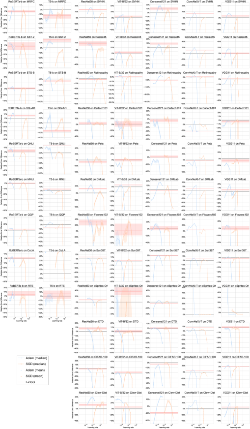
Figure 7: Relative error difference (RED) statistics across seeds (median, mean and IQR shown as shaded region) for all model/task combinations. The red horizontal line shows the median RED of L-DoG.

Model	Optimizer	LR	CoLA	MNLI	MRPC	QNLI	QQP	RTE	SQuAD	SST-2	STS-B	Avg.
RoBERTa-b	Adam	5e-06	60.8	87.8	89.8	93.0	88.7	77.6	90.3	95.1 (0.34)	90.4	85.46
		1e-05	63.4	87.9 (0.05)	90.5	93.1 (0.22)	89.0 (0.11)	77.6	91.5	95.1	90.8	86.22
		3e-05	63.5 (1.33)	87.3	92.3 (0.44)	92.9 (0.15)	88.8	80.6 (1.19)	92.3 (0.05)	94.8 (0.16)	91.1 (0.19)	86.94
		5e-05	61.8	86.8	92.0	92.3	88.0	78.7	92.4 (0.07)	94.3	90.9	85.93
		0.0001	57.5	86.2	91.8	91.3	0.0	79.4	91.9	94.7	89.8	75.33
	SGD	0.003	56.3	86.4	81.9	91.5	85.1	75.5	79.4	93.6	87.0	81.44
		0.01	59.1	87.4	89.7	92.5	87.0	79.0 (0.69)	86.2	94.8	90.3 (0.25)	84.81
		0.03	62.3 (1.38)	87.8 (0.04)	91.8 (0.21)	92.7 (0.18)	88.3	78.9 (0.79)	89.5 (0.12)	95.0 (0.15)	90.7 (0.12)	86.30
		0.1	58.7	87.4	91.0	92.2	88.7 (0.06)	78.3	91.0	94.0	90.4	85.52
		0.3	0.0	86.0	81.2	85.3	87.7	64.6	91.3 (0.11)	92.8	27.0	68.14
		1.0	0.0	81.5	81.2	83.8	79.4	52.7	82.8	89.7	13.0	62.22
	DoG	-	62.8 (1.17)	87.7 (0.12)	91.6 (0.29)	92.6 (0.15)	88.2 (0.02)	78.5 (2.91)	91.3 (0.17)	94.9 (0.26)	90.5 (0.33)	86.46
	L-DoG	-	63.3 (0.32)	87.7 (0.12)	91.5 (0.19)	92.8 (0.28)	88.7 (0.14)	80.1 (1.00)	91.8 (0.18)	94.8 (0.54)	90.6 (0.34)	86.81
T5-b	Adam	5e-06	53.4 (0.93)	86.8	91.4	93.4	88.0	79.8	90.3	93.9	90.4	84.82
		1e-05	56.0 (0.63)	86.9	91.2	93.5	88.2	80.5	90.4	94.2	90.6	85.33
		3e-05	58.9 (1.10)	87.1	91.6	93.4 (0.16)	88.8	82.3	90.8	94.8 (0.24)	90.7	86.12
		5e-05	58.9 (0.80)	87.3	91.8	93.3	89.0	80.9	90.7	94.8	90.8 (0.10)	85.97
		0.0001	58.3 (0.80)	86.9	92.9 (0.35)	93.5 (0.10)	89.2	82.5 (0.48)	90.9 (0.15)	94.9 (0.26)	90.8 (0.18)	86.53
		0.0005	55.4 (0.45)	86.1	92.3	92.7	88.8	81.2 (1.48)	90.0	94.6	89.7	85.29
	SGD	0.003	22.9 (1.64)	85.8	90.1	92.7	87.5	66.8	90.3	92.1	90.3	79.43
		0.01	49.4 (0.27)	86.4	92.2	93.1	87.4	80.9	90.3	93.0	90.5	84.49
		0.03	56.4 (0.52)	86.5	92.0	93.2 (0.03)	88.1	80.9	90.5	93.6	90.6	85.40
		0.1	58.9 (0.82)	86.8	91.8	93.1	88.7	84.1	90.7 (0.04)	93.7	90.6 (0.09)	86.13
		0.3	56.7 (0.83)	86.1	92.8 (0.47)	93.0 (0.13)	88.7	82.8 (1.24)	90.7 (0.05)	93.9 (0.15)	90.7 (0.21)	86.07
		1.0	0.0 (0.00)	32.8	81.2	91.7	56.9	78.7	90.1	92.1	88.7	67.56
	DoG	-	7.3 (6.78)	86.9 (0.21)	92.8 (0.35)	93.1 (0.09)	88.5	81.7 (3.06)	90.6 (0.05)	94.1 (0.19)	90.7 (0.09)	80.58
	L-DoG	-	59.9 (1.43)	87.3 (0.10)	91.9 (0.32)	93.6 (0.02)	87.8	83.1 (0.78)	90.3 (0.02)	95.0 (0.19)	90.5 (0.05)	86.51

Table 4: Average (std) performance of RoBERTa-b and T5-b on language tasks, when fine-tuned with different optimization algorithms and their respective base learning rate (when applicable). DoG uses $r_{\epsilon}=10^{-6}(1+\|x_{0}\|)$ and L-DoG uses $r_{\epsilon}=10^{-8}(1+\|x_{0}\|)$. Scores are reported as mean across seeds, measured in the corresponding performance metric as detailed in Table 3.

Model	Optimizer	LR	Caltech101	CIFAR-100	Clevr-Dist	DMLab	dSprites-Ori	DTD	Flowers102	Pets	Resisc45	Retinopathy	Sun397	SVHN	Avg.
ConvNeXt-T	Adam	3e-06	-	70.0	89.2	70.5	86.5	72.1	92.5	93.1	91.2	-	36.7	-	-
		1e-05	89.0	84.7	91.7	72.7	95.7	70.9	93.5	93.3	94.7	83.2	64.2	96.6	85.33
		3e-05	89.4	87.8	91.4	73.2	96.3	71.3	93.3	92.9	95.6	83.2	74.3	97.3	86.75
		0.0001	87.5	88.5	91.9	76.0	96.4	73.3	93.9	92.6	95.9	83.7	76.0	97.4	87.25
		0.0003	91.1	88.2	93.2	77.5	7.6	72.5	94.3	93.8	96.3	83.9	76.3	97.8	80.58
		0.001	87.5	85.9	93.2	78.5	7.6	69.1	93.4	92.3	95.9	83.5	74.7	97.5	79.42
		0.003	87.6	73.7	90.2	22.2	7.6	63.4	87.9	88.3	94.7	73.6	71.7	19.6	64.50
	SGD	0.01	90.2	85.0	90.8	70.3	7.6	72.0	92.0	94.3	93.4	82.9	68.4	96.2	78.25
		0.03	89.5	87.2	91.1	72.2	7.6	72.6	91.8	94.1	94.8	83.4	74.2	97.0	79.25
		0.1	89.1	87.5	90.9	74.3	7.6	72.3	92.9	94.7	95.4	83.6	75.4	97.2	79.58
		0.3	89.7	87.4	24.5	75.2	7.6	71.4	92.4	93.8	95.9	83.4	75.1	97.3	74.00
		1.0	88.1	86.1	24.5	22.2	7.6	64.0	0.4	13.4	2.1	73.6	74.5	19.6	39.33
		3.0	0.4	1.0	20.0	22.2	7.4	2.1	0.3	2.7	2.2	73.6	0.5	6.7	11.25
		10.0	-	1.0	20.0	22.2	7.4	2.1	0.3	2.7	2.2	-	0.5	-	-
	DoG	-	89.9	87.7	90.7	75.3	7.6	71.6	92.4	93.8	95.5	83.5	75.0	97.3	79.50
	L-DoG	-	87.7	88.2	88.5	76.3	96.4	73.8	92.7	93.7	95.9	83.7	75.9	97.7	86.92
Densenet121	Adam	3e-06	-	62.3	84.3	65.0	84.8	65.9	88.1	88.4	90.6	-	37.9	-	-
		1e-05	86.5 (1.24)	76.9	86.9	66.3	95.4	66.4	88.6	89.7	93.9	81.1	59.6	95.6	81.71
		3e-05	85.2	82.0	89.0	69.0	95.9	66.4 (0.76)	90.0	89.0	94.4	81.0	68.7	96.8	83.70
		0.0001	86.7 (1.40)	82.8 (0.26)	91.4 (0.16)	72.7 (0.69)	96.3 (0.07)	65.8 (0.39)	89.4 (1.08)	89.4 (0.57)	94.8 (0.16)	81.7 (0.10)	70.8 (0.45)	97.3 (0.05)	84.92
		0.0003	84.5	83.3	92.7	76.3	96.4 (0.03)	65.1	88.9	89.2	95.1 (0.20)	82.7	71.6	97.7 (0.08)	84.93
		0.001	81.8	80.8	93.9	76.6 (0.39)	96.4	62.8	87.2	84.7	94.9	83.0 (0.08)	69.7	97.7	83.55
		0.003	76.0	76.7	93.7 (0.17)	74.6	96.0	56.1	81.5	82.7	93.9	82.8	66.2	97.4	81.06
	SGD	0.01	87.7 (0.74)	83.6	89.5	68.5	96.1	65.7	87.4	90.9	94.2	81.6	68.9	96.7	83.73
		0.03	87.0	84.0 (0.08)	91.1	71.4	96.3 (0.07)	66.6 (1.59)	88.6	90.5 (0.47)	94.7	82.0	71.1	97.1	84.87
		0.1	87.9 (0.57)	83.7 (0.31)	92.8 (0.26)	74.5 (0.53)	96.4 (0.05)	65.9 (0.49)	88.3 (0.82)	90.6 (0.28)	94.9 (0.36)	82.5 (0.08)	71.5 (0.21)	97.4 (0.09)	85.53
		0.3	85.5	82.5	92.4 (0.56)	69.1 (3.67)	95.9	62.9	87.6	87.9	95.0 (0.25)	82.6 (0.28)	70.9	97.2	83.67
		1.0	61.6	65.1	91.4	61.9	7.6	35.4	55.4	64.6	82.6	80.0	62.0	95.6	63.17
		3.0	50.1	61.6	88.5	59.2	7.6	23.4	44.1	39.8	85.8	76.5	45.6	94.7	55.92
	DoG	-	87.4 (0.65)	84.0 (0.18)	91.4 (0.19)	71.9 (0.43)	96.2 (0.04)	66.1 (0.90)	88.5 (0.92)	90.3 (0.40)	94.8 (0.12)	82.0 (0.08)	71.6 (0.22)	97.2 (0.13)	85.12
	L-DoG	-	86.9 (0.27)	83.5 (0.18)	89.8 (0.31)	71.5 (0.24)	96.1 (0.03)	66.4 (0.61)	88.7 (0.70)	90.6 (0.13)	95.3 (0.17)	81.9 (0.10)	71.4 (0.25)	97.5 (0.09)	84.97
ResNet50	Adam	0.0003	87.8 (1.52)	84.8	91.0	73.3	96.2	68.5 (0.97)	92.7	93.1 (0.27)	95.5	82.2	73.9	97.0	86.03
		0.001	88.3 (1.18)	83.9 (0.31)	92.4 (0.21)	76.5 (0.53)	96.3 (0.04)	67.2 (0.94)	89.2 (1.83)	92.0 (0.37)	95.5 (0.25)	83.0 (0.18)	73.7 (0.33)	97.6 (0.07)	86.30
		0.003	86.9	83.1	93.3 (0.37)	78.3 (0.30)	96.1	64.4	90.1	90.2	95.4	83.4 (0.15)	72.2	97.7	85.67
		0.01	79.9	75.9	93.5	75.0	95.9	58.0	85.1	85.0	94.4	83.0	66.5	97.4	82.08
		0.03	62.8	64.9	92.4	71.3	95.3	46.9	63.1	67.0	89.3	82.0	50.8	96.4	73.08
	SGD	0.01	86.7	62.9	83.7	52.5	68.3	66.2	80.9	91.9	84.0	75.9	48.0	80.2	72.92
		0.03	86.7	77.0	88.0	63.0	88.5	67.2	82.1	92.8	90.5	78.8	64.7	91.4	80.50
		0.1	87.6 (0.66)	82.8	90.2	67.0	95.5	67.5 (1.71)	89.2	93.5	93.8	81.7	71.6	95.0	84.26
		0.3	87.4	84.8	91.1	70.7	95.9	70.5	85.8 (2.54)	92.9	94.7	82.3	73.9	96.1	84.98
		1.0	86.6 (0.50)	84.5 (0.46)	90.1 (0.51)	72.6 (1.56)	96.0 (0.08)	66.4 (1.16)	85.5 (2.39)	93.0 (0.30)	94.6 (0.28)	82.6 (0.09)	73.6 (0.44)	96.8 (0.06)	85.19
		3.0	87.4	84.7	91.8	70.1	96.0	66.9	90.3	92.1	94.8 (0.49)	82.1	73.7	97.0 (0.10)	85.23
		10.0	86.2	81.2	91.4 (0.71)	67.2	7.6	59.4	86.6	82.2	94.6	78.2	70.0	96.9	74.78
		30.0	0.4	12.1	20.0	22.2	7.4	24.1	43.6	16.5	83.6	73.6	3.1	6.7	25.75
	DoG	-	86.8 (0.62)	84.8 (0.37)	89.3 (0.58)	71.4 (0.77)	95.7 (0.09)	66.4 (1.48)	85.8 (2.64)	92.9 (0.38)	94.6 (0.33)	82.6 (0.16)	73.5 (0.41)	96.5 (0.10)	85.02
	L-DoG	-	87.6 (1.15)	84.6 (0.38)	90.8 (0.38)	75.0 (0.44)	96.0 (0.05)	69.1 (1.30)	90.2 (2.02)	92.4 (0.36)	95.6 (0.46)	82.2 (0.15)	74.6 (0.32)	97.4 (0.08)	86.29
VGG11	Adam	3e-06	80.2 (0.71)	-	-	-	-	-	-	-	-	79.8 (0.07)	-	93.8 (0.15)	-
		1e-05	80.5	73.7	89.3	63.5	94.3	61.5	82.1	87.3	91.4	80.0	65.4	95.3	80.00
		3e-05	82.2 (0.48)	74.9	90.5	67.7	96.1 (0.06)	61.4 (0.84)	84.0	88.1 (0.17)	92.9	81.1	66.6	96.4	81.48
		0.0001	82.6	75.6 (0.23)	92.4	71.9	7.6	61.6	83.5 (1.06)	87.2	93.5 (0.23)	82.3	66.9 (0.12)	96.8	74.79
		0.0003	82.3	74.1	93.2 (0.25)	74.4 (0.47)	7.5	59.6	83.0	86.0	93.4	82.9 (0.08)	66.3	96.8 (0.14)	74.77
		0.001	61.7	61.1	24.5	64.6	7.5	48.0	53.7	65.0	89.1	73.6	50.5	96.5	57.58
		0.003	-	1.0	89.4	68.4	7.6	2.1	0.5	2.7	76.2	-	30.5	-	-
		0.01	-	1.0	24.5	22.2	7.6	2.1	1.2	2.7	2.2	-	2.0	-	-
	SGD	0.001	81.0	68.5	85.0	62.3	14.8 (3.59)	61.3	80.3	88.0	89.3	78.9	61.9	92.0	71.65
		0.003	81.8	72.4	90.3	64.2	12.3	62.2	80.9	88.0	90.9	80.3	64.9	94.4	73.08
		0.01	82.4	73.5	91.9 (0.19)	67.0	9.8	61.2	82.0 (0.99)	89.0 (0.37)	91.7	81.7	65.8	95.7	73.91
		0.03	83.0 (0.50)	74.7 (0.21)	92.1 (0.19)	69.1 (0.36)	7.6 (0.04)	61.9 (0.41)	82.3 (1.09)	89.4 (0.32)	92.5 (0.28)	82.2 (0.06)	66.1 (0.10)	96.4 (0.08)	74.77
		0.1	49.6 (44.91)	74.6 (0.08)	20.0	22.2	7.6	60.5	0.3	87.5	2.2	73.6	53.2 (29.49)	6.7	37.87
		0.3	-	1.0	20.0	22.2	7.4	2.1	0.3	2.7	2.2	-	0.5	-	-
		1.0	-	1.0	20.0	22.2	7.4	2.1	0.3	2.7	2.2	-	0.5	-	-
	DoG	-	82.9 (0.45)	74.7 (0.22)	91.5 (0.17)	68.4 (0.53)	10.4 (0.82)	62.5 (1.19)	82.8 (0.95)	89.5 (0.23)	92.4 (0.22)	81.6 (0.07)	66.3 (0.33)	96.3 (0.09)	74.94
	L-DoG	-	82.4 (0.60)	74.8 (0.16)	92.0 (0.11)	69.9 (0.44)	92.1 (8.59)	62.6 (0.95)	82.7 (1.15)	88.9 (0.62)	92.4 (0.15)	81.9 (0.18)	65.8 (0.09)	96.5 (0.12)	81.83
ViT-B/32	Adam	3e-06	90.7 (0.76)	92.3 (0.22)	89.5 (0.35)	66.0 (0.69)	94.0 (0.24)	74.9 (0.24)	98.5 (0.53)	91.6 (0.11)	95.5 (0.07)	79.7 (0.08)	75.5 (0.23)	96.8 (0.06)	87.08
		1e-05	90.2 (0.47)	92.8 (0.21)	89.9 (0.52)	67.5	51.5 (48.10)	76.9	98.7 (0.29)	90.7	96.3	79.8	78.0 (0.12)	97.6	83.84
		3e-05	88.6	92.5	89.7	70.1	7.6	75.3 (0.24)	98.7	91.6 (0.21)	96.5 (0.13)	80.1 (0.09)	78.3	97.7	80.21
		0.0001	89.5	91.2	89.1	70.8 (0.32)	7.6	72.9	98.1	90.0	96.1	80.1	77.0	97.8 (0.07)	79.80
		0.0003	87.9	87.3	87.9	68.5	7.6	69.0	94.9	87.9	94.9	79.3	72.5	97.9	77.33
		0.001	80.3	62.1	88.1	51.2	7.6	50.4	71.0	58.3	88.6	73.6	53.6	96.3	64.75
		0.003	-	13.5	64.6	29.3	7.6	14.1	26.7	12.1	71.9	-	19.5	-	-
	SGD	3e-05	-	6.1	52.7	40.8	32.7	45.9	61.4	80.3	59.7	-	5.2	-	-
		0.0001	85.0	73.7	71.3	50.4	57.0	69.0	98.1	90.1	83.0	75.3	24.7	79.1	71.17
		0.0003	88.7	88.7	83.1	60.3	69.6	74.7	98.8	91.9	90.2	76.6	59.6	90.7	80.50
		0.001	90.8	91.7	88.1	65.6	87.5	74.8	98.7 (0.51)	93.0 (0.21)	93.5	78.2	73.4	95.2	85.48
		0.003	90.9 (0.89)	92.8 (0.10)	87.3 (1.28)	66.3 (0.40)	85.6 (15.77)	75.3 (0.29)	98.9 (0.31)	92.5 (0.27)	95.3 (0.10)	79.4 (0.02)	77.3 (0.16)	96.6 (0.17)	86.52
		0.01	90.7 (0.63)	92.9 (0.14)	85.9	68.8	56.1	75.2	99.3	92.5	95.8	79.7	78.9 (0.08)	97.4	84.04
		0.03	89.8	92.5	83.1	69.7 (0.29)	65.8	75.8 (0.59)	99.3	92.2	96.2 (0.06)	78.9 (2.51)	78.3	97.7 (0.05)	84.69
		0.1	88.0	91.2	25.2	22.2	7.6	74.9	98.7	91.0	95.9	73.6	76.8	97.8	69.75
		0.3	0.4	1.0	24.5	22.2	7.6	70.5	1.8	2.7	2.3	73.6	0.5	19.6	18.42
	DoG	-	89.5 (1.26)	92.5 (0.22)	85.0 (0.27)	69.5 (0.11)	67.7 (36.66)	75.5 (0.71)	98.9 (0.25)	92.4 (0.16)	96.4 (0.10)	79.7 (0.01)	77.8 (0.13)	97.7 (0.08)	85.22
	L-DoG	-	89.6 (0.81)	92.8 (0.15)	86.0 (0.40)	70.7 (0.29)	95.3 (0.08)	75.8 (0.71)	99.0 (0.26)	92.3 (0.45)	96.5 (0.17)	79.8 (0.07)	78.3 (0.26)	97.8 (0.04)	87.82

Table 5: Average (std) test accuracy across seeds for vision tasks, when fine-tuned with different optimization algorithms and their respective base learning rate when applicable. DoG and L-DoG use $r_{\epsilon}=10^{-4}(1+\|x_{0}\|)$.

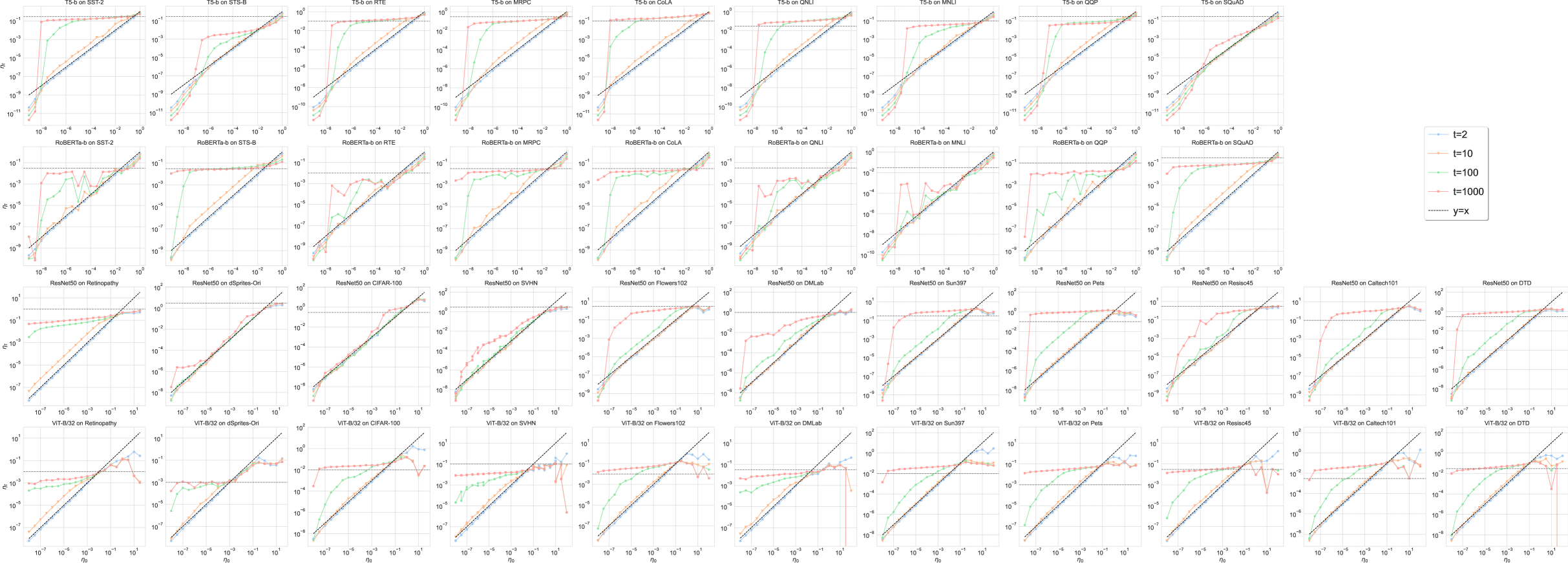
Figure 8: Stabilizing behavior of DoG on $\eta_{t}$ as a function of $\eta_{0}$ ($x$-axis) and $t$ (color). In most cases $\eta_{t}$ quickly stabilizes around a value close to the optimal SGD base learning rate (dashed horizontal line) for all sufficiently small $\eta_{0}=r_{\epsilon}/\|g_{0}\|$. The main exceptions (where $\eta_{t}$ depends strongly on $\eta_{0}$) are dSprites-Ori, CIFAR-100 and SVHN when trained with ResNet50; see F.4 for further discussion.

F.2 Comparison with equalized compute budget

Throughout the paper, our experiments focus on comparing different methods by the final test performance they are able to reach given sufficient compute budget to essentially fully converge. As a consequence, SGD and Adam—which require learning rate tuning—use up significantly more computation than DoG and L-DoG. More specifically, for each model/task combination we tune the SGD and Adam learning rates over a grid of at least 5 values (and often 6 or more), resulting in computational cost increased by the same factor.

In this subsection only, we compare different optimizers using roughly the same computational budget, by measuring the performance of Adam and SGD after roughly 20% of their overall step budget. Figure 9 shows the result of this comparison, contrasting it to our main experiment. The figure shows that DoG often exceeds the performance of instance-tuned SGD with equalized step budget.

We note a number of caveats regarding the equalized compute budget comparison:

1. Since our experiments are focused on getting the best possible generalization, we substantially over-provisioned the iteration budget, and hence the performance of instance-tuned SGD and Adam declines only mildly when we cut the budget by roughly 5. Our tightest budget was for RoBERTa (150% the iterations in Liu et al. [54]), and there we can see that performance degraded more substantially. If we were to instead take the number of iterations DoG actually needs to reach its peak performance, its advantage over equalized-compute SGD would likely be far larger.

2. Since the results reported here are obtained by re-analysis of our original experiments, the cosine learning rate schedule for SGD and Adam is not properly set for using 20% of the iteration budget; in particular, the learning rate does not decay to zero at the end of the training. Running these methods with a properly set cosine schedule would likely improve their performance. However, we note that the addition of iterate averaging appears to partially compensate for the lack of sharp learning rate decay.

3. Given sufficient resources, it is possible to run all the different learning rates of SGD and Adam in parallel. Therefore, the comparison equalizes overall computational cost, but not necessarily wall time.

4. The comparison also does not take into account more sophisticated learning rate tuning schemes that early-stop unpromising learning rate candidates. However, such schemes run the risk of choosing a suboptimal learning rate.

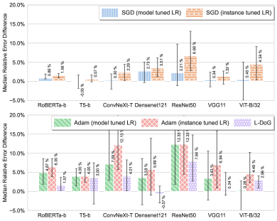
(a) SGD/Adam have $>5$x the DoG/L-DoG budget.

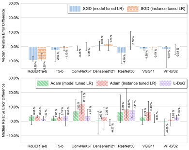
(b) SGD/Adam have roughly the same budget as DoG/L-DoG

Figure 9: RED median (bar chart) and IQR (error bars) of each model on the set of applicable tasks, where we either (a) give the same iteration budget for each optimizer run, resulting in SGD and Adam using more than 5x total compute than DoG and L-DoG due to learning rate tuning (this is a reproduction of Figure 3), or (b) give each algorithm roughly equal compute budget by running SGD and Adam (with 5 or more learning rates) for roughly 20% of the steps that DoG and L-DoG use. With equalized compute budget, DoG outperforms model-tuned SGD almost always and often outperforms the instance-tuned SGD as well, while L-DoG closes most of the gap to Adam.

F.3 Fine-tuning CoLA

As discussed in Section 4.2, DoG with $r_{\epsilon}=10^{-6}(1+\|x_{0}\|)$ failed in fine-tuning T5-b on CoLA. To investigate this issue, we ran DoG and L-DoG with different choices of $r_{\epsilon}$. Figure 11 depicts the results of this experiment as well as the performance of SGD and Adam with different learning rates. The figure shows that using lower values of $r_{\epsilon}$ allows DoG to reach reasonable results, but with some seeds still failing. In contrast, L-DoG shows consistent and superior performance across a large range of $r_{\epsilon}$ values. We leave further investigations on the cause of failure in CoLA to future work.

F.4 Sensitivity of DoG to $r_{\epsilon}$ and the effect of batch normalization

In Section 4.3, we discuss DoG’s insensitivity to the choice of $r_{\epsilon}$ as long as it is small enough. Here, we expand on this analysis by testing how the DoG step size at iteration $t$, denoted $\eta_{t}$, depends on its initial step size $\eta_{0}=r_{\epsilon}/\|g_{0}\|$. For each task in our testbed and for 4 models, we perform short training runs with a large number of $\eta_{0}$ values. In Figure 8 we plot $\eta_{t}$ vs. $\eta_{0}$ for $t\in\{2,10,100,1000\}$. We also show a horizontal line for the learning rate of of SGD reaching the best validation accuracy, and the $y=x$ diagonal. The figure shows that for most model/task combinations, $\eta_{t}$ converges quickly (within the first $1000$ steps) to a value near the optimal one for SGD, and mostly independent of $\eta_{0}$ as long as it is small enough.

However, we also observe some failure cases where $\eta_{t}$ strongly depends on $\eta_{0}$, such as fine-tuning ResNet50 on CIFAR-100. This provides a complementary perspective on the fact DoG is sensitive to $r_{\epsilon}$ in this setting, as already shown in Figure 3: when $\eta_{0}$ is to low, DoG fails to reach a suitable value of $\eta_{t}$ in a reasonable time. We hypothesize that this is due to the batch normalization (BN) layers in the model causing many different step size to “look” like solutions to the implicit equation motivating DoG. To test this hypothesis, we repeat the CIFAR-100 training experiment but without BN (we disable BN by fine-tuning the model in evaluation mode). Figure 10(a) shows that removing BN allows DoG to recover its stabilizing behavior. Moreover, Figure 10(b) further shows that without batch normalization, the performance of DoG again becomes insensitive to the choice of $r_{\epsilon}$ provided it is sufficiently small. Unsurprisingly, we also observe that removing BN slightly hurts generalization performance in this task. As mentioned in Section 6, improving DoG to be more robust in the presence of normalization layers in general and batch normalization in particular is an important direction for future research.

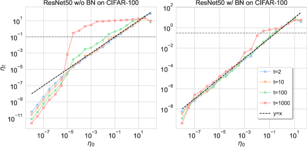
(a)

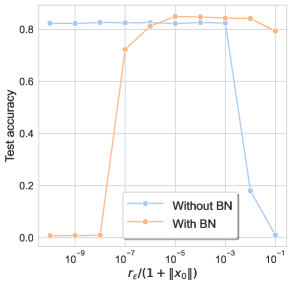
(b)

Figure 10: ResNet50 fine-tuned on CIFAR-100 with and without batch normalization. The dashed horizontal line indicates the best SGD learning rate. (a) Stabilizing behavior of DoG on $\eta_{t}$ as a function of $\eta_{0}$ ($x$-axis) and $t$ (color). Turning off batch normalization (left) mitigates the sensitivity of $\eta_{t}$ to $\eta_{0}$ observed in batch normalized model (right). (b) Accuracies of models trained with DoG (for 20K steps) as a function of $r_{\epsilon}$. Without batch normalization, DoG is robust to smaller values of $r_{\epsilon}$.

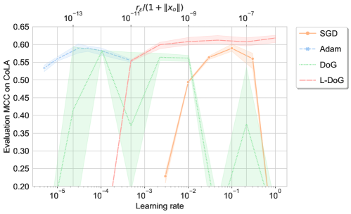
Figure 11: Matthews correlation of T5-base fine-tuned on CoLA with SGD and Adam with different base learning rates (bottom axis), as well as with DoG and L-DoG with different $r_{\epsilon}$ (top axis). Only L-DoG and Adam perform consistently well across different parameters. The lines and shaded regions show the average Matthews correlation and the min-max range, respectively, computed over 3 seeds.

F.5 The growth rate of $\bar{r}_{t}$

Figure 12 plots $\bar{r}_{t}$ for DoG as a function of the iteration index $t$. As the figure shows, $\bar{r}_{t}$ grows very rapidly and then approximately plateaus. Therefore, the quantity $\sum_{i\leq t}\frac{\bar{r}_{i}}{\bar{r}_{t}}$ grows roughly linearly in $t$, implying a near-optimal rate of convergence for DoG, as discussed in Section 3.2.

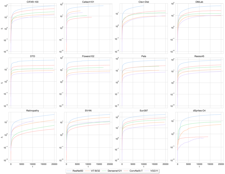
Figure 12: The quantity $\bar{r}_{t}=\max_{i\leq t}{\lVert x_{i}-x_{0}\rVert}$ as a function of the number of steps $t$ in our computer vision testbed. The value of $\bar{r}_{t}$ grows rapidly at first and then almost plateaus.

Appendix G Comparison to Other Tuning-Free Methods

Section 4.7 discusses a comparison between DoG and other parameter-free optimizers. In this section, we provide further details on the experiments.

G.1 Parameter-free SGD

Carmon and Hinder [11] propose a bisection procedure for tuning the SGD learning rate. A direct implementation of this method would need to perform at least 4 or 5 bisection steps and therefore, in the best case, perform similarly to our instance-tuned SGD baseline. Since our learning rate tuning employs a tight grid of values selected using some prior knowledge of the problem, and since we select learning rates based on validation set performance and not a step size certificate, instance-tuned SGD is likely a conservative upper bound on the performance of bisection approach.

Similar to instance tuned SGD, the bisection procedure has increased computational cost relative to DoG that is due to the need for multiple SGD runs. That is, performing 5 steps of bisection where each SGD call has the same step budget as DoG consumes 5 times more compute than DoG. We may also consider a situation where each bisection step uses only 20% of the DoG compute budget, leading to equal overall cost. In this setting, the “equalized compute budget” comparison we perform in Section F.2 and Figure 9 provides a conservative upper bound on the bisection performance, indicating it is likely to under-perform DoG.

G.2 Stochastic Polyak step-size

We apply the Stochastic Polyak Step (SPS) proposed by Loizou et al. [56] using their open-source implementation to a subset of our fine-tuning testbed, and present the results in Sections G.4 and G.4. For the vision experiments, the SPS with the hyper-parameters proposed in the paper ($c=0.2$, $\tau=2$) and initial step size of 1.0 (the default in the code) worked reasonably well, but not as well as DoG. For the language experiments the same algorithm diverges; we find initial learning rate of 0.01 worked reasonably well, but again not as well as DoG (we also attempted an initial learning rate of 0.0001, which produced worse results). For vision tasks, similarly tuning the initial step size did not significantly improve performance. We run 5 random seeds per experiment, and average the results across seeds. DoG outperforms SPS in 22 out of 34 task/model combinations, and by 2.3 percentage points on average. L-DoG further increases this gap by outperforming SPS in 24 out of 34 pairs, with an average of 5.3 percentage points.

G.3 D-adaptation

Empirical comparison to D-adapt SGD and Adam.

We perform a preliminary empirical evaluation of the practical algorithms proposed in Defazio and Mishchenko [25] using the code they release and a subset of our fine-tuning testbed. As Sections G.4 and G.4 show, D-adapt SGD and and D-adapt Adam perform reasonably well but slightly worse than DoG, and noticeably worse than L-DoG and Adam. DoG outperforms D-adapt SGD in 24 out of 34 task/model combinations, and by 1.9 percentage points on average. L-DoG further increases this gap by outperforming D-adapt SGD in 30 out of 34 pairs, with an average of 4.9 percentage points. D-adapt Adam is less stable on many of the tasks in our testbed, being outperformed by DoG in 26 out of 34 task/model combinations, and by L-DoG in 27, with an average of 10.8 and 13.8 percentage points respectively.

Theoretical comparison to Algorithm 1 of Defazio and Mishchenko [25].

Defazio and Mishchenko [25] carry out their main theoretical analysis on a “Parameter Free Dual Averaging” (PFDA) method. We now provide some additional remarks comparing PFDA and DoG. The iterate $x_{t}$ in PFDA is

$$x_{t}=x_{0}-\frac{1}{\sqrt{G_{t}}}\sum_{i\leq t}q_{i}g_{i}$$

where $G_{t}=\sum_{i\leq t}\|g_{i}\|^{2}$ and $q_{i}$ is a lower bound on the distance to optimality (denoted $d_{i}$ in [25]). In contrast, the DoG iterates are

$$x_{t}=x_{0}-\sum_{i\leq t}\frac{\bar{r}_{i}}{\sqrt{G_{i}}}g_{i}$$

where $\bar{r}_{t}=\max_{i\leq t}\|x_{i}-x_{0}\|$. While both $d_{t}$ in PFDA and $\bar{r}_{t}$ are lower bounds for (a constant factor times) the distance to optimality, only DoG aims to approximate $\eta_{\star}=\frac{\|x_{0}-x_{\star}\|}{\sqrt{G_{t}}}$; PFDA instead approximates the optimal step size for dual averaging.

The dual averaging prescription of putting the factor $1/\sqrt{G_{t}}$ outside the summation defining $x_{t}$ likely hurts performance in practice. The practical D-adapt SGD and D-adapt Adam methods that Defazio and Mishchenko [25] propose do not follow this prescription. Consequently, these algorithms are very different from PFDA and have no theoretical guarantees.

G.4 Continuous Coin Betting

Orabona and Tommasi [71] propose a parameter-free algorithm based on coin-betting schemes and demonstrate its effectiveness in training neural networks. We use an open source implementation to apply COCOB on the same subset of our testbed as the other experiments in this section, and present the results in Sections G.4 and G.4. While the default parameters work well for ResNet50 (slightly better than DoG and similar to L-DoG), they produced poor results on the other models. We found that increasing the $\alpha$ parameter (which roughly corresponds to the number of “warmup” steps) from a constant 100 to 10% of the step budget improves the results dramatically for all transformer-based models, though in most cases DoG continues to significantly outperform it. Additionally, we find that in almost all cases, our averaging scheme benefits COCOB.

Model	Optimizer	CoLA	MRPC	QNLI	RTE	SQuAD	SST-2	Avg.
RoBERTa-b	D-Adapt (Adam)	0.0 (0.00)	83.4 (4.93)	66.7 (22.13)	68.4 (14.40)	7.0 (0.16)	58.2 (17.88)	47.28
	D-Adapt (SGD)	49.4 (27.59)	91.6 (0.43)	91.9 (0.67)	81.4 (1.04)	91.5 (0.13)	94.1 (0.38)	83.32
	SPS	49.8 (6.79)	88.4 (3.21)	91.8 (0.21)	52.7	90.1 (0.10)	94.1 (0.28)	77.70
	COCOB	0.0 (0.00)	81.2 (0.00)	92.5 (0.33)	52.7 (0.00)	1.1 (0.00)	92.0 (1.19)	53.25
	DoG	62.8 (1.17)	91.6 (0.29)	92.6 (0.15)	78.5 (2.91)	91.3 (0.17)	94.9 (0.26)	85.28
	L-DoG	63.3 (0.32)	91.5 (0.19)	92.8 (0.28)	80.1 (1.00)	91.8 (0.18)	94.8 (0.54)	85.72
T5-b	D-Adapt (Adam)	11.1 (2.51)	81.8 (0.65)	85.0 (1.91)	58.1 (1.35)	90.4 (0.06)	87.1 (3.00)	68.92
	D-Adapt (SGD)	0.0 (0.00)	92.5 (0.59)	92.9 (0.04)	81.2 (0.78)	90.4 (0.06)	80.3 (2.67)	72.88
	SPS	39.1 (2.35)	92.9 (1.21)	93.2 (0.10)	80.9 (1.82)	90.5 (0.04)	94.3 (0.31)	81.82
	COCOB	59.2 (1.02)	86.2 (2.93)	93.4 (0.12)	83.5 (1.66)	90.5 (0.05)	94.8 (0.35)	84.60
	DoG	7.3 (6.78)	92.8 (0.35)	93.1 (0.09)	81.7 (3.06)	90.6 (0.05)	94.1 (0.19)	76.60
	L-DoG	59.9 (1.43)	91.9 (0.32)	93.6 (0.02)	83.1 (0.78)	90.3 (0.02)	95.0 (0.19)	85.63

Table 6: Average (std) performance of RoBERTa-b and T5-b on language tasks, when fine-tuned with different optimization algorithms. DoG uses $r_{\epsilon}=10^{-6}(1+\|x_{0}\|)$ and L-DoG uses $r_{\epsilon}=10^{-8}(1+\|x_{0}\|)$. SPS uses $c=0.2$, $\tau=2$ as recommended by Loizou et al. [56], but initial step size of 0.01 as the recommended value 1.0 diverged for some tasks. Still, when fine-tuning RoBERTa-b on RTE, 3 out of 5 training runs diverged; for this case we report the mean of the two successful runs and omit the standard deviation. For COCOB we set $\alpha$ to be 10% of the total steps per task, as the default of $\alpha=100$ failed to outperform a random guess. We measure performance as detailed in Table 3.

Model	Optimizer	Caltech101	CIFAR-100	Clevr-Dist	DMLab	dSprites-Ori	DTD	Flowers102	Pets	Resisc45	Retinopathy	Sun397	SVHN	Avg.
ResNet50	D-Adapt (Adam)	79.0 (1.60)	82.9 (0.23)	92.3 (0.50)	75.2 (0.97)	96.3 (0.01)	60.1 (0.51)	84.6 (1.73)	85.1 (0.95)	94.1 (0.28)	83.4 (0.07)	72.9 (0.11)	97.0 (0.21)	83.58
	D-Adapt (SGD)	86.2 (0.93)	84.3 (0.15)	89.6 (0.60)	74.8 (0.73)	95.9 (0.04)	64.4 (1.31)	84.9 (1.12)	92.0 (0.25)	94.7 (0.17)	82.7 (0.12)	73.0 (0.09)	97.1 (0.06)	84.97
	SPS	86.4 (1.14)	80.2 (1.20)	92.9 (0.25)	76.2 (0.60)	96.0 (0.05)	63.7 (0.83)	84.3 (1.45)	92.4 (0.19)	94.9 (0.22)	83.3 (0.17)	70.9 (0.82)	97.5 (0.03)	84.89
	COCOB	86.3 (1.53)	83.5 (0.21)	87.4 (0.43)	68.4 (0.72)	95.8 (0.03)	66.4 (0.31)	87.0 (1.11)	92.4 (0.35)	93.8 (0.18)	82.0 (0.10)	72.2 (0.16)	96.8 (0.07)	84.33
	DoG	86.8 (0.62)	84.8 (0.37)	89.3 (0.58)	71.4 (0.77)	95.7 (0.09)	66.4 (1.48)	85.8 (2.64)	92.9 (0.38)	94.6 (0.33)	82.6 (0.16)	73.5 (0.41)	96.5 (0.10)	85.02
	L-DoG	87.6 (1.15)	84.6 (0.38)	90.8 (0.38)	75.0 (0.44)	96.0 (0.05)	69.1 (1.30)	90.2 (2.02)	92.4 (0.36)	95.6 (0.46)	82.2 (0.15)	74.6 (0.32)	97.4 (0.08)	86.29
ViT-B/32	D-Adapt (Adam)	87.6 (0.48)	91.8 (0.31)	89.0 (0.42)	70.7 (0.48)	7.6 (0.00)	69.4 (1.55)	94.7 (0.92)	86.6 (1.42)	95.5 (0.32)	80.1 (0.09)	76.2 (0.38)	97.9 (0.05)	78.92
	D-Adapt (SGD)	88.7 (0.58)	91.8 (0.20)	84.2 (2.39)	70.5 (0.17)	44.0 (31.87)	74.9 (0.38)	98.2 (0.43)	91.5 (0.72)	96.3 (0.06)	79.8 (0.05)	76.3 (0.13)	97.7 (0.03)	82.82
	SPS	89.7 (0.51)	91.4 (0.18)	84.6 (1.18)	71.3 (0.27)	7.6 (0.00)	74.4 (0.96)	98.4 (0.33)	91.1 (0.49)	96.2 (0.17)	79.9 (0.09)	77.5 (0.46)	98.0 (0.04)	80.01
	COCOB	89.2 (1.01)	91.5 (0.19)	84.9 (0.88)	70.7 (0.70)	7.6 (0.00)	74.7 (0.92)	98.4 (0.48)	90.8 (0.26)	96.5 (0.12)	80.0 (0.15)	77.1 (0.22)	97.9 (0.07)	79.94
	DoG	89.5 (1.26)	92.5 (0.22)	85.0 (0.27)	69.5 (0.11)	67.7 (36.66)	75.5 (0.71)	98.9 (0.25)	92.4 (0.16)	96.4 (0.10)	79.7 (0.01)	77.8 (0.13)	97.7 (0.08)	85.22
	L-DoG	89.6 (0.81)	92.8 (0.15)	86.0 (0.40)	70.7 (0.29)	95.3 (0.08)	75.8 (0.71)	99.0 (0.26)	92.3 (0.45)	96.5 (0.17)	79.8 (0.07)	78.3 (0.26)	97.8 (0.04)	87.82

Table 7: Average (std) test accuracy across seeds for vision tasks, when fine-tuned with different optimization algorithms. DoG and L-DoG use $r_{\epsilon}=10^{-4}(1+\|x_{0}\|)$. SPS uses $c=0.2$, $\tau=2$ and initial step size of 1 as recommended by Loizou et al. [56]. For COCOB we set $\alpha$ to be 10% of the total steps per task; the default value of $\alpha=100$ performed well on ResNet50 but very badly on ViT-B/32.

References

- Abadi et al. [2015] Martín Abadi, Ashish Agarwal, Paul Barham, Eugene Brevdo, Zhifeng Chen, Craig Citro, Greg S. Corrado, Andy Davis, Jeffrey Dean, Matthieu Devin, Sanjay Ghemawat, Ian Goodfellow, Andrew Harp, Geoffrey Irving, Michael Isard, Yangqing Jia, Rafal Jozefowicz, Lukasz Kaiser, Manjunath Kudlur, Josh Levenberg, Dandelion Mané, Rajat Monga, Sherry Moore, Derek Murray, Chris Olah, Mike Schuster, Jonathon Shlens, Benoit Steiner, Ilya Sutskever, Kunal Talwar, Paul Tucker, Vincent Vanhoucke, Vijay Vasudevan, Fernanda Viégas, Oriol Vinyals, Pete Warden, Martin Wattenberg, Martin Wicke, Yuan Yu, and Xiaoqiang Zheng. TensorFlow: Large-scale machine learning on heterogeneous systems, 2015. URL https://www.tensorflow.org/. Software available from tensorflow.org.
- Agarwal et al. [2012] Alekh Agarwal, Peter L Bartlett, Pradeep Ravikumar, and Martin J Wainwright. Information-theoretic lower bounds on the oracle complexity of stochastic convex optimization. IEEE Transactions on Information Theory, 58(5):3235–3249, 2012.
- Arrow and Enthoven [1961] Kenneth J Arrow and Alain C Enthoven. Quasi-concave programming. Econometrica: Journal of the Econometric Society, pages 779–800, 1961.
- Asi and Duchi [2019] Hilal Asi and John C Duchi. The importance of better models in stochastic optimization. Proceedings of the National Academy of Sciences, 116(46):22924–22930, 2019.
- Bar Haim et al. [2006] Roy Bar Haim, Ido Dagan, Bill Dolan, Lisa Ferro, Danilo Giampiccolo, Bernardo Magnini, and Idan Szpektor. The second PASCAL recognising textual entailment challenge. In Proceedings of the Second PASCAL Challenges Workshop on Recognising Textual Entailment, 2006.
- Beattie et al. [2016] Charles Beattie, Joel Z Leibo, Denis Teplyashin, Tom Ward, Marcus Wainwright, Heinrich Küttler, Andrew Lefrancq, Simon Green, Víctor Valdés, Amir Sadik, et al. Deepmind lab. arXiv:1612.03801, 2016.
- Bentivogli et al. [2009] Luisa Bentivogli, Ido Dagan, Hoa Trang Dang, Danilo Giampiccolo, and Bernardo Magnini. The fifth PASCAL recognizing textual entailment challenge. In Text Analysis Conference (TAC), 2009.
- Bernstein et al. [2020] Jeremy R. Bernstein, Arash Vahdat, Yisong Yue, and Ming-Yu Liu. On the distance between two neural networks and the stability of learning. arXiv:2002.03432, 2020.
- Berrada et al. [2020] Leonard Berrada, Andrew Zisserman, and M Pawan Kumar. Training neural networks for and by interpolation. In International Conference on Machine Learning (ICML), 2020.
- Bhaskara et al. [2020] Aditya Bhaskara, Ashok Cutkosky, Ravi Kumar, and Manish Purohit. Online learning with imperfect hints. In International Conference on Machine Learning (ICML), 2020.
- Carmon and Hinder [2022] Yair Carmon and Oliver Hinder. Making SGD parameter-free. In Conference on Learning Theory (COLT), 2022.
- Carmon et al. [2019] Yair Carmon, Aditi Raghunathan, Ludwig Schmidt, John C Duchi, and Percy S Liang. Unlabeled data improves adversarial robustness. Advances in Neural Information Processing Systems (NeurIPS), 2019.
- Cer et al. [2017] Daniel Matthew Cer, Mona T. Diab, Eneko Agirre, Iñigo Lopez-Gazpio, and Lucia Specia. Semeval-2017 task 1: Semantic textual similarity multilingual and crosslingual focused evaluation. In International Workshop on Semantic Evaluation, 2017.
- Chandra et al. [2022] Kartik Chandra, Audrey Xie, Jonathan Ragan-Kelley, and Erik Meijer. Gradient descent: The ultimate optimizer. Advances in Neural Information Processing Systems (NeurIPS), 2022.
- Chen et al. [2022] Keyi Chen, John Langford, and Francesco Orabona. Better parameter-free stochastic optimization with ODE updates for coin-betting. In AAAI Conference on Artificial Intelligence, 2022.
- Cheng et al. [2017] Gong Cheng, Junwei Han, and Xiaoqiang Lu. Remote sensing image scene classification: Benchmark and state of the art. Proceedings of the IEEE, 105(10):1865–1883, 2017.
- Cimpoi et al. [2014] Mircea Cimpoi, Subhransu Maji, Iasonas Kokkinos, Sammy Mohamed, and Andrea Vedaldi. Describing textures in the wild. In Conference on Computer Vision and Pattern Recognition (CVPR), 2014.
- Comet.ML [2021] Comet.ML. Comet.ML home page, 2021. URL https://www.comet.ml/.
- Cubuk et al. [2019] Ekin D Cubuk, Barret Zoph, Dandelion Mane, Vijay Vasudevan, and Quoc V Le. AutoAugment: Learning augmentation strategies from data. In Conference on Computer Vision and Pattern Recognition (CVPR), 2019.
- Cutkosky [2019] Ashok Cutkosky. Artificial constraints and hints for unbounded online learning. In Conference on Learning Theory (COLT), 2019.
- Cutkosky and Orabona [2018] Ashok Cutkosky and Francesco Orabona. Black-box reductions for parameter-free online learning in Banach spaces. In Conference on Learning Theory (COLT), 2018.
- Dagan et al. [2006] Ido Dagan, Oren Glickman, and Bernardo Magnini. The PASCAL recognising textual entailment challenge. In Machine learning challenges. Evaluating predictive uncertainty, visual object classification, and recognising tectual entailment. Springer, 2006.
- Davis and Drusvyatskiy [2019] Damek Davis and Dmitriy Drusvyatskiy. Stochastic model-based minimization of weakly convex functions. SIAM Journal on Optimization, 29(1):207–239, 2019.