Non-Abelian currents bootstrap

Abstract

We initiate the study of correlation functions of non-Abelian spin-1 conserved current in three dimensional conformal field theories using numerical conformal bootstrap. We discuss the general framework and apply it to the particular cases of $SU(N)$ and $O(N)$ global symmetry. In both cases we obtain general bounds on operator dimensions. In the large-$N$ limit our bounds show features in correspondence of the expected position of fermionic QED₃ in three dimensions, as well as other interesting theories. By imposing gaps inspired by the spectrum of QED₃ at large-$N$, we manage to restrict the plane of certain operator dimensions to a small island, where QED₃ must live.

I Introduction

The conformal bootstrap Rattazzi et al. (2008); Rychkov and Vichi (2009) has proven itself a successful tool which allowed us to precisely determine critical exponents of many conformal field theories (CFTs) Kos et al. (2016); Atanasov et al. (2022); Chester et al. (2020, 2021), such as the O(N) vector model and Gross-Neveu Yukawa CFTs Erramilli et al. (2022) (see also Poland et al. (2019) for a review). Despite the outstanding results obtained, CFTs arising as infrared (IR) fixed points of gauge theories have still eluded any bootstrap attempt to narrow them Chester and Pufu (2016a); Li (2018); He et al. (2021a); Li and Poland (2021); He et al. (2021b); Albayrak et al. (2022); He et al. (2022); Li (2022); Reehorst et al. (2020); Manenti and Vichi (2021).

Quantum electrodynamics in 2+1 dimensions, besides being an interesting theoretical model by itself, is also an interesting model because of its connection to important condensed matter systems. In particular, the IR fixed point of $N=4$ flavors of Dirac fermions coupled to U(1) gauge theory were proposed to describe the so-called U(1) Dirac spin liquid (DSL) phase Affleck and Marston (1987); Wen and Lee (1996); Hastings (2000); Hermele et al. (2005, 2008); Song et al. (2020, 2019). Similar to the famous Kosterlitz–Thouless phase Kosterlitz and Thouless (1973) in 1+1 dimensions, the U(1) Dirac spin liquid phase is a conformal phase of matter. Various theoretical and even real life materials were proposed which could potentially realize the U(1) DSL phase in their phase diagram Song et al. (2020, 2019); Ran et al. (2007); Iqbal et al. (2013, 2016); He et al. (2017); Hu et al. (2019).

The validity of these theoretical predictions and correspondingly the realization of the conformal U(1) DSL phase in nature depend on two necessary conditions: 1) the $N=4$ QED₃ theory indeed flow to an IR conformal fixed point under renormalization, 2) certain operators that are not protected by the lattice symmetry must be irrelevant.

For QED₃ theory with $N$ flavors of Dirac fermions coupled to U(1) gauge theory, it is believed that there exists a critical $N^{critical}$, above which the theory flows to a conformal fixed point. Below $N^{critical}$, on the other hand, the conformal phase is replaced by a gapped phase analogous to the chiral symmetry breaking phase of four dimension Quantum chromodynamics (QCD). Remember that for (4-dimensional) QCD with SU(3) gauge symmetry coupled to $N$ quarks, there also exists a critical $N^{critical}$, above which the theory is believed to flow to the famous Banks-Zaks fixed point Belavin and Migdal (1974); Caswell (1974); Banks and Zaks (1982). Even though there have been many attempts in determining the $N^{critical}$ for 2+1 dimensional QED₃ using various methods Dagotto et al. (1990); Kaveh and Herbut (2005); Grover (2012); Karthik and Narayanan (2016a, b); Giombi et al. (2016); Di Pietro et al. (2016), just like the 3+1D QCD, the number has not been concretely determined, mainly due to the strong coupling nature of the theory.

Among the many models proposed to realize the U(1) Dirac spin liquid, one promising type is the spin-1/2 quantum magnet on various non-bipartite lattices (e.g. kagome and triangular lattice). On these lattices, the lattice model usually preserves a UV symmetry group which is strictly smaller than the symmetry group of the IR conformal QED₃ theory. From the renormalization group flow point of view, this means that if an operator is not protected by symmetry, it will be generated by the Renormalization Group (RG) flow. Since the conformal fixed point lives in the IR of the RG flow, if the operator is an irrelevant operator of the CFT, its coupling constant will grow along the RG flow and eventually will drive the system away from the conformal fixed point. In other words, if the conformal phase of QED₃ can be realized as a conformal phase of these lattice Hamiltonians, all operators allowed by the UV symmetry must be irrelevant.

In order to check both of the necessary conditions concretely, it is very important to study the corresponding CFT non-perturbatively, this makes the conformal bootstrap method a very promising tool to attack this problem. However, even though there have been various attempts to precisely pin-point of $N=4$ QED₃ among the vast region consistent with the bootstrap constraints He et al. (2022); Albayrak et al. (2022), its precise location has not been identified yet. The second necessary condition was used in He et al. (2022) to get lower bounds on the order parameter critical exponents. The lower bounds seem to be consistent with various Monte Carlo studies.

One possible approach to bootstrap QED₃ is to first locate the theory in a certain perturbative limit, where perturbative results provide a concrete guide in the choice of assumptions on the operator dimensions. Indeed, bootstrap islands corresponding to the large-$N$ limits of scalar QED₃ theories has been discovered in He et al. (2021b). After locating QED₃ in the perturbative limits, one may hope to follow the bootstrap islands to the non-perturbative regime by continuously changing the fermion/boson flavor number $N$. Recently, various advanced numerical techniques Reehorst et al. (2021) have made such a calculation possible Benoit et al. (2023).

It is not our goal in this paper to completely solve the problem of bootstrapping QED₃. We will rather try to attack the first part of the problem, finding QED₃ in a bootstrap setup in the large-$N$ limit. One of the main features of CFTs corresponding to gauge theories is the absence of low dimensional scalar operators, since the fundamental fields appearing in the UV Lagrangian are not gauge invariant. Unfortunately conformal bootstrap starts to lose strength when the scaling dimension is far from the unitarity bound, leading to bounds that are not very constraining. On the other hand, a common feature of gauge theories is the presence of conserved currents associated with non-abelian global symmetries. One might hope that considering such universal operators inside correlation functions might lead to stronger constraints.

In the context of supersymmetric CFTs the inclusion of conserved operators is greatly simplified since most conserved currents belong to supersymmetric multiplets also containing scalar operators. Since supersymmetry relates correlation functions of operators in the same multiplet, one can get non trivial constraints by restricting to scalars only. In the general case instead one needs to deal with correlation functions of spinning operators. Previous works have considered conserved spin-1 currents associated to a global abelian $U(1)$ symmetry, both alone Dymarsky et al. (2019) and mixed with a charged scalar Reehorst et al. (2019), as well as the stress tensor Dymarsky et al. (2018). In this work we initiate a systematic study of correlation functions of non-abelian conserved currents. We begin by considering the non-abelian currents alone and study the bounds on the CFT data contributing to this particular four point (4pt) function in the case of $SU(N)$ and $O(N)$ global symmetry. We plan to consider mixed correlation functions in future works. We will comment on this in the conclusions.

One of the main difficulties of the present analysis is that any CFT with a given global symmetry represents a solution of our crossing equations, it being free, bosonic, fermionic, based on gauge theory or not. Thus, in order to focus on a specific theory it is important to get a rough intuition of its expected spectrum and how it differs from other CFTs. After reviewing the general setup in Sec. II, we will concentrate on the case of $SU(N)$ and $O(N)$ global symmetries in Sec. III and Sec. IV. At the beginning of each section we discuss possible assumptions that can distinguish among gauge theories in the large-$N$ limit and less interesting free theories (more details are also given in Appendix A). Next, we present various bounds that apply to the space of all CFTs with a given global symmetry. Finally, in order to focus on a specific theory, we will impose ad-hoc assumptions on the CFT spectrum and obtain more stringent bounds. Appendix B contains a detailed review of the bootstrap constraints for four identical currents, while Appendix C generalizes the analysis to the non abelian case and Appendix D formulates the boostrap problem.

II Setup

In this work we consider the constraints arising from imposing CFT axioms on the 4pt functions of four conserved currents associated to a global symmetry $\mathcal{G}$.

Since the current $J^{a}_{\mu}$ satisfies Ward identities, its normalization is fixed by this condition. Hence the two point function normalization acquire a physical meaning, as for the stress energy tensor:

$$\langle J_{\mu}^{a}(x)J_{\nu}^{b}(0)\rangle=C_{J}\frac{\eta_{\mu\nu}-2\frac{x_{\mu}x_{\nu}}{x^{2}}}{x^{2(d-1)}}\delta^{ab}\,.$$ (1)

The coefficient $C_{J}$ is called current central charge.

Whenever we take the diverge of $J_{\mu}^{a}$, up to contact terms, one has the conservation condition

$$\langle\partial^{\mu}J_{\mu}^{a}(x)\mathcal{O}_{1}(x_{1})\ldots\mathcal{O}_{n}(x_{n})\rangle=0.$$ (2)

for any set of operators $\mathcal{O}_{i}(x_{i})$. As we review in the appendices, when restricted to 3pt function, the above conditions translates to an algebraic relation among OPE coefficients involving $J$, while when imposed on 4pt function, it produces a set of differential equations linking some of the functions parametrizing the correlator.

In Appendix B we first review the bootstrap setup for abelian currents and we generalize it to the non-abelian case in Appendix C. In the main text we will maintain a schematic notation. Since currents transform in the adjoint representation of $\mathcal{G}$ we have the schematic OPE

$$J_{\mu}^{a}\times J_{\nu}^{b}\sim\sum_{r\in Adj\otimes Adj}\widetilde{T}_{r}^{ab,A}\sum_{\mathcal{O}}\sum_{i=1}^{n_{3}}\lambda_{JJO}^{(i)}\widetilde{Q}_{i}^{\mu\nu,\alpha_{1}\ldots\alpha_{\ell}}\mathcal{O}^{A}_{\alpha_{1}\ldots\alpha_{\ell}}\,.$$ (3)

In the above expression we denoted $\widetilde{T}_{r}^{ab,A}$ a tensor in flavor space that converts adjoint indices $a,b$ to representation $r$ indices, collectively denoted $A$. Similarly $\widetilde{Q}_{i}^{\mu\nu,\alpha_{1}\ldots\alpha_{\ell}}$ translates the vector indices $\mu,\nu$ to spin-$\ell$ representation. Notice that for a given operator there are multiple OPE coefficients $\lambda_{JJO}^{(i)}$: this is different from the OPE of two scalar operators.

Similarly, we write the 4pt correlation function as

$$\langle J_{\mu}^{a}(x_{1})J_{\nu}^{b}(x_{2})J_{\rho}^{c}(x_{3})J_{\sigma}^{d}(x_{4})\rangle=\sum_{r}\sum_{s=1}^{n_{4}}\mathcal{K}_{4}(x_{i})T_{r}^{abcd}\mathcal{Q}_{\mu\nu\rho\sigma}^{(s)}(x_{i})g_{s}^{(r)}(u,v)\,,$$ (4)

$$\mathcal{K}_{4}(x_{i})=x_{12}^{-4}x_{34}^{-4},\quad u=\frac{x_{12}^{2}x_{34}^{2}}{x_{13}^{2}x_{24}^{2}},\quad v=\frac{x_{14}^{2}x_{23}^{2}}{x_{13}^{2}x_{24}^{2}},\quad x_{ij}^{2}=(x_{i}^{\mu}-x_{j}^{\mu})(x_{i}^{\mu}-x_{j}^{\mu})\,,$$ (5)

where the sum over $r$ represents a finite sum over irreducible representations of $\mathcal{G}$ while $s$ labels the independent tensor structures $\mathcal{Q}_{\mu\nu\rho\sigma}^{(s)}(x_{i})$ one can construct using four points. The number of independent four point structures is $n_{4}=41$ when $J$’s are non-conserved currents, the number will be greatly reduced if $J$ is conserved. Finally $T_{r}^{abcd}$ are invariant tensors of the flavor symmetry group. The indices $a,b,c,d$ live in the adjoint representation of the flavor symmetry group, the superscript $r$ denotes the irreducible representations that appears in the (reducible) tensor product representation $Adj\otimes Adj$ (10). $T_{r}^{abcd}$ are projectors that project the $Adj\otimes Adj$ (10) into invariant sub-spaces that correspond to the irreducible representations. The conformal invariant functions $g_{s}^{(r)}(u,v)$ also admit a conformal block decomposition in terms of operators in a given flavor symmetry irreducible representation, as in (3). The coefficients in such an expansion are related to the OPE coefficients in (3). The details will be discussed in Appendix B and C.

II.1 Special operators in $J^{a}_{\mu}\times J^{b}_{\nu}$

As reviewed in Appendix B.1, in the case of abelian currents, there are no spin-1 operators appearing in the OPE $J\times J$, neither parity even, nor parity odd. One important novelty in the present setup is instead the possibility to access these operators. In particular, $J^{a}_{\mu}$ appears in its own OPE. Following Li et al. (2016) we can parametrize the 3pt function $\langle J_{\mu}^{a}(x_{1})J_{\nu}^{b}(x_{2})J_{\rho}^{c}(x_{3})\rangle$ using the embedding formalism Costa et al. (2011a) (see appendix B for all definitions)

$$\langle J^{a}(P_{1},Z_{1})J^{b}(P_{2},Z_{2})J^{c}(P_{3},Z_{3})\rangle=f^{abc}\frac{\lambda_{1}V_{1}V_{2}V_{3}+\lambda_{2}(V_{1}H_{23}+H_{13}V_{2}+H_{12}V_{3})}{(-2P_{1}\cdot P_{2})^{\frac{3}{2}}(-2P_{1}\cdot P_{3})^{\frac{3}{2}}(-2P_{2}\cdot P_{3})^{\frac{3}{2}}}\,,$$ (6)

where $P_{i},Z_{i}$ are coordinates and polarizations in the embedding space. Using Ward identities one can relate the coefficients $\lambda_{1},\lambda_{2}$ to the current central charge $C_{J}$ and a second parameter:

$$\lambda_{1}=\frac{3C_{J}}{S_{3}}-5\lambda_{JJJ}\,,\qquad\lambda_{2}=-\lambda_{JJJ}\,.$$ (7)

Here $S_{d}$ is the volume of the $(d-1)$ dimensional sphere $S_{d}=\frac{2\pi^{d/2}}{\Gamma(d/2)}$. An important point we should stress is that the 3pt function of three conserved currents is parametrized by 2 independent coefficients while the 3pt function of two currents and a generic non-conserved parity even spin-1 operator by only one.

Another important operator is the stress tensor, which appears in the parity even singlet sector:

$$\langle J^{a}(P_{1},Z_{1})J^{b}(P_{2},Z_{2})T(P_{3},Z_{3})\rangle=\delta^{ab}\frac{\lambda_{1}V_{1}V_{2}V_{3}^{2}+\lambda_{2}H_{12}V_{3}^{2}+\lambda_{3}(V_{1}H_{23}+H_{13}V_{2})+\lambda_{4}H_{13}H_{23})}{(-2P_{1}\cdot P_{2})^{\frac{1}{2}}(-2P_{1}\cdot P_{3})^{\frac{1}{2}}(-2P_{2}\cdot P_{3})^{\frac{1}{2}}}\,.$$ (8)

A convenient parametrization of the coefficients $\lambda_{i}$ is Li et al. (2016); Dymarsky et al. (2019):

$$\lambda_{1} =-\left(7+108\gamma\right)C\,, \lambda_{2} =(5+36\gamma)C\,, C= \frac{3}{32\pi}C_{J}\,,$$

$$\lambda_{3} =-6(1+4\gamma)C\,, \lambda_{4} =2\left(1-12\gamma\right)C\,.$$ (9)

We recall that the parameter $\gamma$ is subject to the conformal collider bounds $|\gamma|\leq 1/2$, as shown in Hofman and Maldacena (2008).

III $SU(N)$ currents

After the general introduction of the previous sections, let us now concentrate on two cases of interest: in this section we analyze theories with a global $SU(N)$ global symmetry, while the next section will focus on $O(N)$ symmetry. In a similar fashion as for the case of abelian currents Dymarsky et al. (2019), it is possible to obtain bounds on the smallest dimension operator with a given spin, parity and transforming in a given irreducible representation of the global symmetry group. In the main text we only present plots relevant to the discussion.

III.1 OPE and targets

The tensor product of two $SU(N)$ adjoint representations $Adj_{i}$, i.e. rank-2 traceless tensors with one index in the fundamental and one in the anti-fundamental, is given by

$$Adj_{1}\times Adj_{2}=S^{+}+Adj^{+}+S\bar{S}^{+}+A\bar{A}^{+}+Adj^{-}+S\bar{A}^{-}+A\bar{S}^{-}\,.$$ (10)

Here $S$ and $Adj$ refer to $SU(N)$ singlet and adjoint representations. Instead $A\bar{A}$, $S\bar{S}$, $S\bar{A}$, $S\bar{A}$ are rank-4 tensors with two upper and two lower indices. The naming convention refers to whether the upper and lower indices are symmetric (S) or antisymmetric (A). In addition the label $\pm$ refers to the symmetry properties under exchange of the irreps $Adj_{i}$. In the case of OPE of scalars, this would translate into the parity of spins exchanged in a given representation. In the case of spinning operators the connection is less straightforward and is outlined in Appendix C.

Below we will use the notation (Space-time Parity, Group representation, Spin) to refer to the OPE channels. For example, $(-,S,\ell=2)$ means parity odd, $SU(N)$ singlet, and $\ell=2$ channel.

Since our approach is very general, our bounds will contain all CFTs with an $SU(N)$ global symmetry, including free theories of fermions, free theories of scalars and generalized free fields (GFFs) of currents. The latter are defined as a conserved current of dimension $d-1$ and standard two point function, while all other correlation functions are defined though Wick contractions. All these theories only contain operators with integer dimension.

In order to focus on more interesting interacting theories one has to carefully understand the expected spectrum of the target theory and hopefully identify a series of assumptions that eliminates unwanted solutions. Let us focus on the difference among QED₃, GNY and QCD₃ at large-$N$.

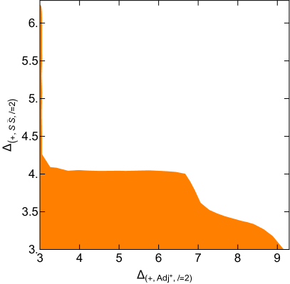
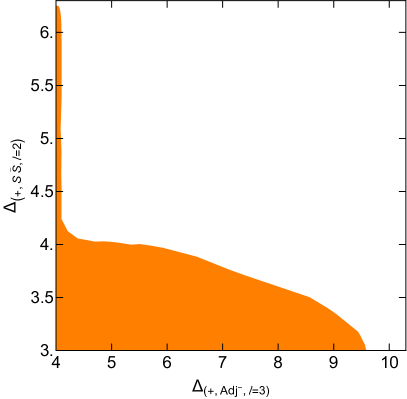
Figure 1: The lowest operator in the $(+,S\bar{S}$, $\ell=2)$ sector v.s. the sector $(+,Adj^{+},\ell=2)$ and $(+,Adj^{-},\ell=3)$: $SU(100)$ CFT. $\Lambda=19$ and no gap is imposed.

The key feature distinguishing QED₃ from QCD₃ is in the leading operators in the $(+,S\bar{S},\ell=2)$ sector, where QED₃ and QCD₃ take values around 6 and 4 respectively. This difference is due to the fact QED₃ has no color index. In the Lagrangian picture, in order to construct such an operator in QED₃, some derivatives need to be inserted, which increases the scaling dimension. Such a mechanism to distinguish different color groups is explained in Reehorst et al. (2020); Manenti and Vichi (2021) and in He et al. (2021b), where the operator is called the decoupling operator. Demanding a large gap closer to 6 in the sector $(+,S\bar{S},\ell=2)$, we are left with QED₃, free fermion and GNY. Finally, a sharp difference between GNY and QED₃ is that GNY has a singlet scalar of dimension 2, while QED₃ has no relevant singlet scalar at large-$N$. In the next section we make use of these expectations to strengthen our bounds and zoom on QED₃ at large-$N$.

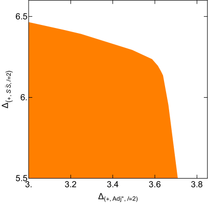
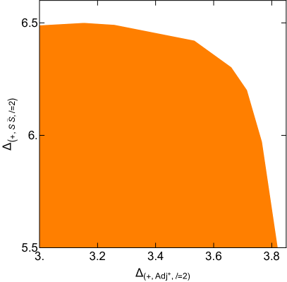
Figure 2: The lowest operator in the $(+,S\bar{S}$, $\ell=2)$ sector v.s. the sector $(+,Adj^{+},\ell=2)$: $SU(4)$ and $SU(3)$ CFT. $\Lambda=19$ and small gaps in several sectors are imposed: $(+,S,\ell=0)\geq 3$, $(+,Adj^{+},\ell=0)\geq 2$, $(+,A\bar{A},\ell=0)\geq 2$, $(+,S\bar{S},\ell=0)\geq 3$. These gaps are topological, namely the numerical bounds will not change if the gaps are either relaxed or tightened up.

III.2 Numerical results

Let us begin with a general bound on spin $\ell=2,3$ operators in the adjoint and $S\bar{S}$ representation at large-$N$, say $N=100$. As shown in Fig. 1 these bounds contain several features, the most peculiar being a prominent spike in the dimensions of the smallest operator in the $(+,S\bar{S},\ell=2)$ sector. As observed in the previous subsection, a large gap in the $S\bar{S}$ sector is expected in the free fermion theory and in QED₃. These bounds imply that once we demand a large gap for the $S\bar{S}$ spin 2 operator, a slightly broken higher spin current has to be present in the spectrum. When the gap for the $S\bar{S}$ spin 2 operator is relaxed to around 4, we observe a kink, where higher spin currents are strongly broken. This corresponds to the GFF solution.

In Fig. 3 we compare the position of the kink with the prediction for the anomalous dimension of the slightly broken higher spin current of Zhou and He (2022) in presence of additional assumptions and we observe a good agreement. The sharp spikes evolve to smoother kinks for smaller values of $N$, as shown in Fig. 2, but in this case the large-$N$ prediction cannot be trusted.

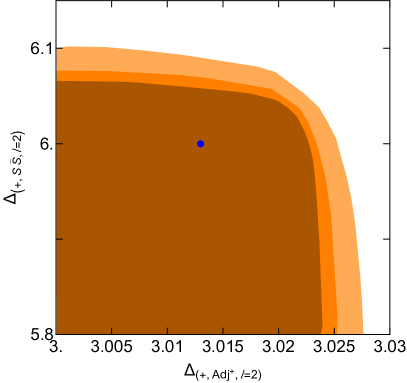
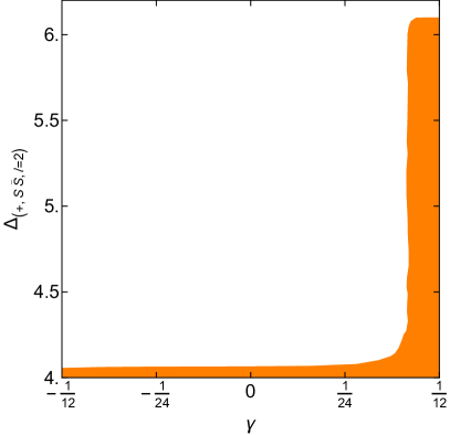
Figure 3: Left panel: The lowest operator in the $(+,S\bar{S}$, $\ell=2)$ sector v.s. the sector $(+,Adj^{+},\ell=2)$: $SU(100)$ CFT. $\Lambda=19,23,27$ and mild gaps in several sectors are imposed: $(+,S,\ell=0)\geq 3$, $(+,Adj,\ell=0)\geq 2$, $(+,A\bar{A},\ell=0)\geq 2$, $(+,S\bar{S},\ell=0)\geq 3$. Right panel: $\gamma$ versus the lowest operator in the $(+,S\bar{S}$, $\ell=2)$ sector: $SU(100)$ CFT. $\Lambda=19$ and mild gaps in several sectors are imposed: $(+,S,\ell=0)\geq 3$, $(+,S,\ell=2)_{2nd}\geq 3.5$, $(+,Adj,\ell=0)\geq 2$, $(+,A\bar{A},\ell=0)\geq 2$, $(+,S\bar{S},\ell=0)\geq 3$. These gaps are topological, namely the numerical bounds will not change if the gaps are either relaxed or tightened up.

The fact that a large gap in the $S\bar{S}$ sector corresponds to a theory resembling the free fermion is also suggested by the bound in Fig. 3. There we bound the dimension of the lowest operator in the $(+,S\bar{S}$, $\ell=2)$ sector v.s. the parameter $\gamma$ defined in (II.1). We recall that the ANEC imposes the constraints $|\gamma|\leq 1/12$, where the two extremes are saturated by free theories. For free fermion, it is known $\gamma=1/12$ Osborn and Petkou (1994). We observed a sharp pike around $\gamma=1/12$. It’s likely that QED₃ sits on the top of the pike with $\gamma<1/12$. In this bound we also add a gap of 3 in the scalar singlet, in principle to avoid a contamination from the GNY model.

We conclude this subsection by observing that the present setup, if combined with the correlation functions of scalars in the adjoint representation (namely the parity odd fermion bilinear $\bar{\psi}_{i}\psi_{j}$) has the potential to create an island with minimal assumptions. Indeed, the request $\Delta_{(+,S\bar{S},\ell=2)}\sim 6$ in the single correlator bootstrap of adjoint scalars forces $\Delta_{\bar{\psi}\psi}\gtrsim 2$ (assuming the bounds has the usual GFF behavior); on the other hand our setup requires $\Delta_{\bar{\psi}\psi}\equiv\Delta_{(-,Adj,\ell=0)}\lesssim 2$, see Fig. 4. This tension might result in a small allowed region.

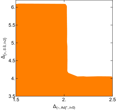
Figure 4: The lowest operator in the $(+,S\bar{S}$, $\ell=2)$ sector v.s. the sector $(-,Adj^{+},\ell=0)$: $SU(100)$ CFT. $\Lambda=19$ and mild gaps in several sectors are imposed: $(+,S,\ell=0)\geq 3$, $(+,Adj,\ell=0)\geq 2$, $(+,A\bar{A},\ell=0)\geq 2$, $(+,S\bar{S},\ell=0)\geq 3$. .

Table 1: Approximate dimension (up to $1/N$ corrections) of operators in QED₃ and free fermion theory. The highlighted sectors distinguish the two theories In particular, one can add proper gaps in the red (blue) sectors to exclude the free fermion theory (QED₃). We also write down the schematic form of operators.

Operator sector	Dimension	QED3	Free fermion
$(+,S,\ell=0)$	$\Delta=4$	$(\bar{\psi}\psi)^{2}$, $F_{\mu\nu}^{2}$	$(\bar{\psi}\psi)^{2}$, $(\bar{\psi}\gamma_{\mu}\psi)^{2}$
$(-,S,\ell=0)$	$\Delta=2$	$(\bar{\psi}\psi)$	$(\bar{\psi}\psi)$
$(+,S,\ell=2)$	$\Delta=3$	$\bar{\psi}\gamma_{\mu}\partial_{\nu}\psi$	$\bar{\psi}\gamma_{\mu}\partial_{\nu}\psi$
	$\Delta=4$	$J^{top}_{\mu}J^{top}_{\nu}$	$(\bar{\psi}\gamma_{\mu}\psi)(\bar{\psi}\gamma_{\nu}\psi)$
$(-,S,\ell=2)$	$\Delta\leq 4$	None	None
$(+,Adj,\ell=0)$	$\Delta=4$	$(\bar{\psi}\psi)(\bar{\psi}^{i}\psi_{j})$	$(\bar{\psi}\psi)(\bar{\psi}^{i}\psi_{j})$, $(\bar{\psi}\gamma_{\mu}\psi)(\bar{\psi}^{i}\gamma_{\mu}\psi_{j})$
	$\Delta=5$	$(\partial_{\nu}F_{\mu\nu})(\bar{\psi}^{i}\gamma_{\mu}\psi_{j})$	None
$(-,Adj,\ell=0)$	$\Delta=2$	$\bar{\psi}^{i}\psi_{j}$	$\bar{\psi}^{i}\psi_{j}$
	$\Delta=4$	$(\bar{\psi}^{i}\gamma_{\mu}\psi_{j})J_{\mu}^{top}$	None
$(+,Adj,\ell=1)$	$\Delta=2$	$\bar{\psi}^{i}\gamma_{\mu}\psi_{j}$	$\bar{\psi}^{i}\gamma_{\mu}\psi_{j}$
	$\Delta=4$	$(\bar{\psi}^{i}\psi_{j})J_{\mu}^{top}$, $(\bar{\psi}^{i}\gamma_{\mu}\psi_{j})F_{\mu\nu}$	None
$(-,Adj,\ell=1)$	$\Delta\leq 3$	None	None
$(+,Adj,\ell=2)$	$\Delta=3$	$\bar{\psi}^{i}\gamma_{\mu}\partial_{\nu}\psi_{j}$	$\bar{\psi}^{i}\gamma_{\mu}\partial_{\nu}\psi_{j}$
	$\Delta=4$	None	$(\bar{\psi}\gamma_{\mu}\psi)(\bar{\psi}^{i}\gamma_{\nu}\psi_{j})$
$(-,Adj,\ell=2)$	$\Delta=4$	$(\bar{\psi}^{i}\gamma_{\mu}\psi_{j})J_{\nu}^{top}$	None
$(+,A\bar{A},\ell=0)$	$\Delta=4$	$\bar{\psi}^{2}\psi^{2}$	$\bar{\psi}^{2}\psi^{2}$
	$\Delta=6$	$\bar{\psi}^{2}\partial^{2}\psi^{2}$	$\bar{\psi}^{2}\partial^{2}\psi^{2}$

III.3 An island for QED₃

In this section we show how it is possible to create an island that is consistent with QED₃ but excludes the free fermion theory. In order to do this we need to impose aggressive assumptions on the spectrum. Let us justify them.

In the large-$N$ limit, the spectrum of QED₃ and free fermions are quite similar, with very few distinct features. Both theories have such $SU(N)$ flavor current. However, QED₃ also has a parity odd topological U(1) current

$$J_{\text{top}}^{\mu}\sim\varepsilon^{\mu\nu\rho}F_{\nu\rho}\,,$$ (11)

while the free fermion theory has a parity even U(1) current $\bar{\psi}\gamma^{\mu}\psi$. In the QED₃ theory one can still write the operator $\bar{\psi}\gamma^{\mu}\psi$: it is, however, a descendent of the topological current due to the equation of motion,

$$e^{2}\bar{\psi}\gamma^{\nu}\psi\sim\partial_{\mu}F^{\mu\nu}\,.$$ (12)

Thus, when classifying operators of QED₃ in the large-$N$ limit, one should use the above identification.

As shown in Table 1, there are various gap features to distinguish QED₃ from free fermion theory. We tried to explore whether free fermion theory can be excluded by exploiting those differences. The simplest setup corresponds to assume the existence of an isolated operator in the $(+,Adj,\ell=2)$ sector, with dimension $\Delta_{(+,Adj,\ell=2)}$, input a gap $\Delta\gtrsim 5$ for the next operator and then scan the value of $\Delta_{(+,Adj,\ell=2)}$ together with other quantities. Unfortunately this setup is not sufficient to exclude the free fermion solution, at least not at $\Lambda\leq 23$.

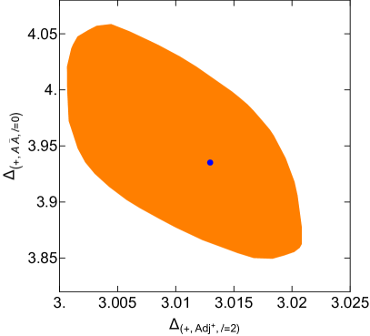
Figure 5: An island of $SU(100)$ CFT in the ($\Delta_{(+,A\bar{A},\ell=0)}$, $\Delta_{(+,Adj,\ell=0)})$ space, which excludes the free fermion theory and is consistent with QED₃. The blue dot corresponds to the large-$N$ value Zhou and He (2022); Chester and Pufu (2016b) of $N=100$ QED₃. $\Lambda=23$ and the specific condition for the setup is in Appendix E.

In order to restrict the space of allowed solution we impose a form of a spectrum close to the expected spectrum at large-$N$. The idea is to demand that operators should exist only within certain intervals centered around the large-$N$ prediction for QED₃. We take $N$ to be large and the size of the interval to be $10/N$. This assumption, together with the gap discussed in the previous paragraph turns out to be sufficient to exclude the free fermion solution, leaving an island in the plane $(\Delta_{(+,A\bar{A},\ell=0)},\Delta_{(+,Adj,\ell=2)})$ consistent only with QED₃.

The result at $\Lambda=23,N=100$ is shown in Figure 5. If we relax the derivative order to $\Lambda=19$, the free fermion theory won’t be excluded. It would be very interesting to see how the island converges at very large $\Lambda$. We leave it for the future.

IV $O(N)$ currents

Let us now move to the case of $O(N)$ global symmetry currents.

Table 2: Expected spectrum for theories with $O(N)$ symmetry up to 1/N correction. The first column indicates the parity, irrep and spin of the operator.

Operator	Free boson	WF	free fermion	GNY	GVFF	bQCD	fQCD
$(+,S,0)$	1	2	4	2	4	2	4
$(+,T,0)$	1	1	4	3	4	1	4
$(+,Q1,0)$	8	8	7	7	4	4	7
$(-,Q1,0)$	5	5	5	5	5	5	5
$(+,Q1,2)$	6	6	4	4	4	4	4
$(+,Q2,0)$	4	4	4	4	4	4	4
$(+,Q2,2)$	4	4	6	6	4	4	4

IV.1 OPE and targets

The tensor product of $O(N)$ adjoint $A$, i.e. rank-2 antisymmetric tensor, is

$$A\times A=S^{+}+T^{+}+Q1^{+}+Q2^{+}+A^{-}+Q3^{-}.$$ (13)

$S$ refers to singlet, $T$ refers to rank-2 symmetric traceless tensor, $Q1,Q2,Q3$ are rank-4 tensors, and the superscript $\pm$ refers to symmetric or antisymmetric tensor product. The dimensions of the three rank-4 tensors are

$$\textrm{dim}[Q1] =\frac{1}{24}(N-3)(N-2)(N-1)N,$$ (14)

$$\textrm{dim}[Q2] =\frac{1}{12}(N-3)N(N+1)(N+2),$$ (15)

$$\textrm{dim}[Q3] =\frac{1}{8}(N-3)(N-1)N(N+2).$$ (16)

It is worth noting that $Q1$ is a fully antisymmetric rank-4 tensor, so for $N=4$ it becomes the pseudo-singlet, namely it is $SO(4)$ singlet but is odd under the improper $Z_{2}$ of $O(4)$.

Theories with the $O(N)$ conserved current include free boson, free fermion, $O(N)$ Wilson-Fisher, $O(N)$ Gross-Neveu-Yukawa theory, generalized vector free field theory, and $SO(N_{c})$ (or $O(N_{c})$) gauge theories. 

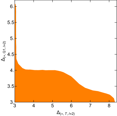
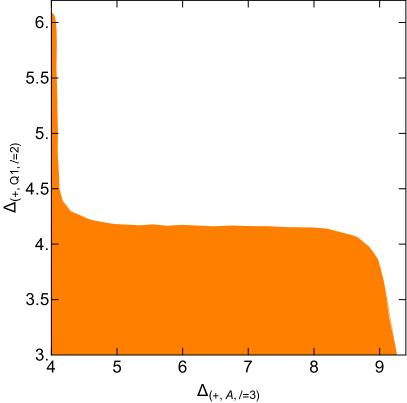
Figure 6: The lowest operator in the $(+,Q1,\ell=2)$ sector v.s. the sector $(+,T,\ell=2)$ and $(+,A,\ell=3)$: $O(100)$ CFT. $\Lambda=19$ and no gap is imposed.

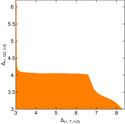
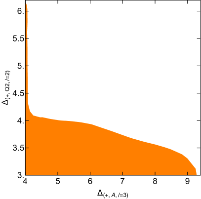
Figure 7: The lowest operator in the $(+,Q2,\ell=2)$ sector v.s. the sector $(+,T,\ell=2)$ and $(+,A,\ell=3)$: $O(100)$ CFT. $\Lambda=19$ and no gap is imposed.

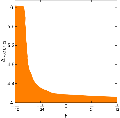
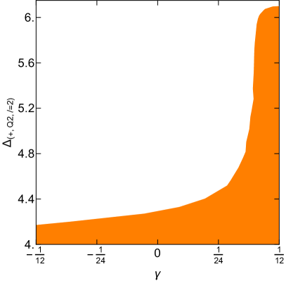
Figure 8: $\gamma$ v.s. the lowest operator in the $(+,Q1,\ell=2)$ or $(+,Q2,\ell=2)$ sector: $O(100)$ CFT. $\Lambda=19$ and mild gaps are imposed: $(+,S,\ell=0)\geq 1$, $(+,S,\ell=2)_{2nd}\geq 3.5$, $(+,Q_{1},\ell=0)\geq 3$, $(+,Q_{2},\ell=0)\geq 3$. These gaps are topological, namely the numerical bounds will not change if the gaps are either relaxed or tightened up.

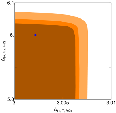
Figure 9: Haunting $O(100)$ GNY CFT: $\Delta_{(+,T,\ell=2)}$ v.s. $\Delta_{(+,Q2,\ell=2)}$. $\Lambda=19,23,27$ and strong gaps in several sectors are imposed: $(+,S,\ell=0)\geq 1.5$, $(+,S,\ell=2)_{2nd}\geq 3.5$, $(+,Q1,\ell=0)\geq 6.5$, $(+,Q1,\ell=2)\geq 3.5$, $(+,T,\ell=0)\geq 3.5$, $(+,Q2,\ell=0)\geq 3.5$, $(+,A,\ell=1)_{2nd}\geq 2.5$.

Table 2 lists several low lying operators that appear in the $J\times J$ OPE. It is worth noting that the lowest operators in certain sectors have dimension that vary substantially depending on the theory. For instance, the sector $(+,Q1,2)$ distinguishes free boson and Wilson-Fisher from all other theories such as fermionic theories, GVFF and QCD₃. Similarly, the leading operator in the $(+,Q2,2)$ sector distinguishes free fermion and GNY from all other theories such as bosonic theories, GVFF and QCD₃.

IV.2 Numerical results

We begin by exploring the bounds on the lowest operators in sectors $(+,Q1,2)$ and $(+,Q2,2)$ discussed in the previous section. The peaks shown in Fig. 6 and Fig. 7 correspond precisely to the large gaps expected in these sectors. In Fig. 8 and 9 further study these peaks by considering the upper bound as a function of the parameter $\gamma$ defined in (II.1), imposing additional gaps in various sectors: this verifies that the peaks correspond to either bosonic theories ($\gamma\sim-1/12$) or fermionic theories ($\gamma\sim 1/12$).

Therefore, as in the case of $SU(N)$, imposing a large gap in the sectors $(+,Q1/Q2,2)$ localizes the value of gamma toward the ends the allowed interval and it imposes the presence of slightly broken higher-spin currents.

Finally, in Fig. 9 we compare the allowed region and the prediction from large-$N$ for two operators. We imposed a set of assumptions to remove the contamination from theories except for GNY. We observe that the peak is not far from the large-$N$ prediction Manashov and Skvortsov (2017), but the convergence in $\Lambda$ is still slow.

V Discussion

In this work, we considered the correlation functions of four conserved spin-1 currents associated with a non-abelian global symmetry. We systematically analyzed the consequences of conservation and permutations for three and four point functions and presented a complete set of linearly independent crossing equations. We applied the machinery of numerical conformal bootstrap, focusing on the case of $SU(N)$ or $O(N)$ symmetry. In both cases, we obtained bounds on scaling dimensions of certain operators. We presented general bounds, which are valid for any unitary CFT in $3d$, but also considered ad-hoc assumptions, which allowed us to focus on specific cases of interest.

One of the main motivations for the present work was to study the IR fixed point of QED₃. To achieve this, we analyzed the spectrum of various theories with $SU(N)$ symmetry at large-$N$, looking for distinct features that allow us to single out QED₃ from other solutions of crossing equations. We identified several such characteristics: a large gap in the parity even, spin-2 sector of the $SU(N)$ representation $S\bar{S}$, and a mild gap between the first and second operator in the parity-even, spin-2, adjoint representation.

We presented bounds on the scaling dimension of the first $S\bar{S}$ spin 2 operator as a functions of various quantities and we observed a sharp pike in the allowed region: it is tempting to identify this peak with the location of QED₃. We also observed that by demanding the $S\bar{S}$ spin 2 operator has dimension around 6, slightly broken higher spin currents must exist in the theory.

In order to completely isolate QED₃ we had to impose aggressive assumptions on the spectrum in the form of narrow intervals centered around the large-$N$ predictions. This assumption is somewhat justified at large-$N$ and allowed us to create a closed region in parameter space which excludes the free theory solution.

In order to go beyond this result, especially for small values of $N$ where anomalous dimensions are expected to be $O(1)$, we will need an effective way to distinguish the QED₃ from free fermion. One way is to include in the bootstrap setup correlators of QED₃ operators that do not exist in the free fermion. Possible candidates are the topological current and monopole operators.

Given the encouraging results of this work, it would be very interesting to obtain more large-$N$ predictions for more low lying operators, especially those transforming in more involved irreducible representations, as well as additional parameters, such as $\gamma$ and $\lambda_{JJJ}$.

Appendix A Operator spectrum of theories with non-Abelian current

Our strategy is the following. We first calculate the partition function for the theories we care about. The partition function is the plethystic exponential of single particle characters, which was used in Meneses et al. (2019) to calculate the partition function of free theory in four dimensions. The SO(3) character for the global symmetry can be written as

$$\chi_{\ell}(x)=\sum_{i=-2\ell}^{2\ell}x^{i},$$ (17)

then the conformal character for a generic (long) multiplet can be written as

$$\chi_{\Delta,\ell}(q,x)=\frac{q^{\Delta}\chi_{\ell}(x)}{(1-q)(1-q/x)(1-qx)}.$$ (18)

The numerator corresponds to the conformal primary, while the denominator comes from the $\partial_{\mu}$’s acting on the conformal primary. For free theory scalar saturating the unitarity bound, due to shortening condition, the character becomes

$$\chi^{short}_{\Delta=1/2,\ell=0}=\chi_{1/2,0}(q,x)-\chi_{5/2,0}(q,x).$$ (19)

The partition function for free theory can then be written as

$$Z(q,x,a)=\text{PE}[\chi^{short}_{\Delta=1/2,\ell=0}(q,x)\cdot\chi_{V}(a)].$$ (20)

Here PE stands for “plethystic exponential”. The character $\chi_{V}(a)$ is the character for the global symmetry, which indicates that the scalar field is in the vector representation of O(N). For details of the characters of O(N), see Appendix B of Henriksson (2023). Expanding the above partition function in terms consisting of conformal characters times the character for the global symmetry (which depends on the global symmetry representation), we get degeneracies of operators at each level. For Wilson-Fisher fixed point at large-$N$, one need to perform the Hubbard-Stratonovich transformation,

$$Z(q,x,a)=\text{PE}[\chi^{short}_{\Delta=1/2,\ell=0}(q,x)\cdot\chi_{V}(a)-\chi_{1,0}(q,x)+\chi_{2,0}(q,x)].$$ (21)

The partition function for other theories (at their perturbative limits) can be worked out in a similar manner. Since the partition function calculation doesn’t tell us about parity symmetry, we still need to enumerate operators to understand their parity symmetry.

Appendix B Review: abelian case

B.1 3pt functions in embedding formalism

In this section we construct the most generic 3pt function of two spin-1 conserved currents and a generic parity even/odd traceless symmetric operator in a CFT in $d=3$. We do this using the embedding formalism developed in Costa et al. (2011a, b).

Let us begin by introducing our basis of tensor structures in embedding space:

$$H_{ij}=\frac{(Z_{i}\cdot Z_{j})(P_{i}\cdot P_{j})-(Z_{i}\cdot P_{j})(P_{i}\cdot Z_{j})}{(P_{i}\cdot P_{j})}\,$$ (22a)

$$V_{i,jk}=\frac{(Z_{i}\cdot P_{j})(P_{i}\cdot P_{k})-(Z_{i}\cdot P_{k})(P_{i}\cdot P_{j})}{\sqrt{{-2(P_{i}\cdot P_{j})(P_{i}\cdot P_{k})(P_{j}\cdot P_{j})}}}\,$$ (22b)

$$V_{1}=V_{1,23}\,\qquad V_{2}=V_{2,31}\,\qquad V_{3}=V_{3,12}\,$$ (22c)

$$\epsilon_{ij}=\varepsilon_{ABCDE}P^{A}_{i}P^{B}_{j}Z_{1}^{C}Z_{2}^{D}Z_{3}^{E}\,.$$ (22d)

where $P_{i}^{A},Z_{i}^{A}$ are $d+2$ dimensional vectors representing the position and polarization vectors in embedding space. We can choose them such that $P_{i}^{2}=Z_{i}^{2}=P_{i}\cdot P_{i}=0$.

The 3pt function of two currents and a third operator is

$$\langle J_{1}(P_{1},Z_{1})J_{2}(P_{2},Z_{2})\mathcal{O}_{\Delta,\ell}(P_{3},Z_{3})\rangle=\frac{\mathcal{T}_{\ell}(P_{i},Z_{i})}{(-2P_{1}\cdot P_{2})^{2-\Delta/2}(-2P_{1}\cdot P_{3})^{\Delta/2}(-2P_{2}\cdot P_{3})^{\Delta/2}}$$ (23)

where the tensor structure for parity even operators reads

$$\mathcal{T}_{0}(P_{i},Z_{i})=\lambda_{1}V_{1}V_{2}+\lambda_{2}H_{12}$$ (24)

$$\mathcal{T}_{1}(P_{i},Z_{i})=\lambda_{1}V_{1}V_{2}V_{3}+\lambda_{2}V_{1}H_{23}+\lambda_{3}H_{13}V_{2}+\lambda_{4}H_{12}V_{3}$$ (25)

$$\mathcal{T}_{\ell}(P_{i},Z_{i})=\lambda_{1}V_{1}V_{2}V_{3}^{\ell}+\lambda_{2}V_{1}H_{23}V_{3}^{\ell-1}+\lambda_{3}H_{13}V_{2}V_{3}^{\ell-1}+\lambda_{4}H_{13}H_{23}V_{3}^{\ell-2}+\lambda_{5}H_{12}V_{3}^{\ell}$$ (26)

and we have suppressed the explicit dependence of the OPE coefficients $\lambda_{i}$ on the 3pt functions operators.

For non-abelian currents we will be interested in the case in which the 3pt function is both symmetric or antisymmetric under exchange of the currents at point 1 and 2. Hence we will analyze the two cases separately. Imposing the correct behavior under permutation and conservation at point 1 and 2, we get the relations among the OPE coefficients summarized in Table 3 and Table 4.

spin	Parity-even: Symmetric & cons			$\#$ ind
$\ell=0$	$\lambda_{2}=-\frac{(2-\Delta)\lambda_{1}}{\Delta}$			1
$\ell=1$		$\lambda_{i}=0$		0
$\ell>0$ even	$\lambda_{1}=-\frac{\lambda_{2}(-\Delta+\ell+4)}{\Delta-2}-\frac{\lambda_{5}(-\Delta-\ell)}{\Delta-2}$;	$\lambda_{3}=\lambda_{2}$;	$\lambda_{4}=\frac{\lambda_{5}\ell}{-\Delta+\ell+2}-\frac{(\Delta-1)\lambda_{2}}{-\Delta+\ell+2}$	2
$\ell>1$ odd		$\lambda_{i}=0$		0

Table 3: OPE relations for conserved currents, symmetric under exchange $1\leftrightarrow 2$, and a third parity-even operator with spin-$\ell$

spin	Parity-even: Anti-sym & cons			$\#$ ind
$\ell=0$		$\lambda=0$		0
$\ell=1$	$\lambda_{1}=(\Delta+3)\lambda_{2}$;	$\lambda_{3}=\lambda_{2}$;	$\lambda_{4}=(\Delta-1)\lambda_{2}$	1
$J$		$\lambda_{2}=\lambda_{3}=\lambda_{4}$		2
$\ell>0$ even		$\lambda_{i}=0$		0
$\ell>1$ odd	$\lambda_{1}=-\frac{\lambda_{2}(-\Delta+\ell+4)}{\Delta-2}-\frac{\lambda_{5}(-\Delta-\ell)}{\Delta-2}$ ;	$\lambda_{3}=\lambda_{2}$ ;	$\lambda_{4}=\frac{\lambda_{5}\ell}{-\Delta+\ell+2}-\frac{(\Delta-1)\lambda_{2}}{-\Delta+\ell+2}$	2

Table 4: OPE relations for conserved currents, antisymmetric under exchange $1\leftrightarrow 2$, and a third parity-even operator with spin-$\ell$. Here $J$ represents a conserved spin-1 current at point 3. Notice that there is one extra OPE coefficient compared to a generic spin-1 non-conserved operator. This is because the rank of the linear relations among OPE coefficients is smaller for $\Delta=2,\ell=1$ compared to the generic case. The same phenomenon appears in $\langle TTT\rangle$.

The tensor structure for parity odd operators instead has the following form

$$\mathcal{T}_{\ell}(P_{i},Z_{i})=\lambda_{1}\varepsilon_{13}V_{2}V_{3}^{\ell-1}+\lambda_{2}\varepsilon_{23}V_{1}V_{3}^{\ell-1}+\lambda_{3}\varepsilon_{13}H_{23}V_{3}^{\ell-2}+\lambda_{4}\varepsilon_{23}H_{13}V_{3}^{\ell-2}$$ (27)

$$\mathcal{T}_{0}(P_{i},Z_{i})=\lambda_{1}\varepsilon_{12}$$ (28)

$$\mathcal{T}_{1}(P_{i},Z_{i})=\lambda_{1}\varepsilon_{13}V_{2}+\lambda_{2}\varepsilon_{23}V_{1}+\lambda_{3}\varepsilon_{12}V_{3}$$ (29)

Notice that for $\ell>1$ we removed one of the $\varepsilon_{ij}$ in terms of the other two using the liner relation

$$\varepsilon_{12}V_{3}^{2}(P_{1}\cdot P_{2})-\varepsilon_{12}(H_{13}+V_{1}V_{3})(P_{2}\cdot P_{3})+\varepsilon_{13}(H_{23}+V_{2}V_{3})(P_{1}\cdot P_{3})=0$$ (30)

which follows from the fact that in $d=5$ dimensions, any six vectors are linearly dependent Costa et al. (2011a).

Imposing the correct behavior under permutation and conservation at point 1 and 2, we get the relations among the OPE coefficients summarized in Table 5 and Table 6.

spin	Parity-odd: Symmetric & cons			$\#$ ind
$\ell=0$		/		1
$\ell=1$		$\lambda_{i}=0$		0
$J$		$\lambda_{i}=0$		0
$\ell>0$ even	$\lambda_{2}=-\lambda_{1}$,	$\lambda_{3}=-\frac{(3-\Delta)\lambda_{1}}{\Delta-\ell-3}$;	$\lambda_{4}=\frac{(3-\Delta)\lambda_{1}}{\Delta-\ell-3}$	1
$\ell>1$ odd	$\lambda_{2}=\lambda_{1}$,	$\lambda_{3}=\frac{(\Delta-1)\lambda_{1}}{\Delta-\ell-3}$;	$\lambda_{4}=\frac{(\Delta-1)\lambda_{1}}{\Delta-\ell-3}$	1

Table 5: OPE relations for conserved currents, symmetric under exchange $1\leftrightarrow 2$, and a third parity-odd operator with spin-$\ell$

spin	Parity-odd: Anti-sym & cons			$\#$ ind
$\ell=0$		$\lambda_{1}=0$		0
$\ell=1$	$\lambda_{2}=-\lambda_{1}$;	$\lambda_{3}=(\Delta-3)\lambda_{1}$;		1
$J$		$\lambda_{2}=\lambda_{3}=-\lambda_{1}$		1
$\ell>1$ even	$\lambda_{2}=\lambda_{1}$,	$\lambda_{3}=\frac{(\Delta-1)\lambda_{1}}{\Delta-\ell-3}$;	$\lambda_{4}=\frac{(\Delta-1)\lambda_{1}}{\Delta-\ell-3}$	1
$\ell>0$ odd	$\lambda_{2}=-\lambda_{1}$ ,	$\lambda_{3}=-\frac{(3-\Delta)\lambda_{1}}{\Delta-\ell-3}$ ;	$\lambda_{4}=\frac{(3-\Delta)\lambda_{1}}{\Delta-\ell-3}$	1

Table 6: OPE relations for conserved currents, antisymmetric under exchange $1\leftrightarrow 2$, and a third parity-odd operator with spin-$\ell$

B.1.1 From embedding to $SO(3)$-basis

In this appendix we work out the change of basis between the embedding frame used in the previous section and the $SO(3)$ basis used by block_3d Erramilli et al. (2021).

Let us begin by introducing the projection from the embedding frame to the conformal frame. For three points we can choose:

$$x_{1}=(0,0,0)$$

$$x_{2}=(0,0,1)$$

$$x_{3}=(0,0,\infty)$$

In addition, we introduce polarization spinors

$$s_{i}=\begin{pmatrix}\xi_{i}\\ \eta_{i}\end{pmatrix}$$ (31)

The projection to this frame can be achieved by the choice of embedding vectors (see Erramilli et al. (2021), appendix F)

$$P^{A}_{1}=(0,0,0,\frac{1}{2},\frac{1}{2})$$

$$P^{A}_{2}=(0,0,1,0,1)$$

$$P^{A}_{3}=(0,0,0,-\frac{1}{2},\frac{1}{2})$$ (32)

$$Z^{A}_{1}=\left(\frac{\xi_{1}^{2}+\eta_{1}^{2}}{\sqrt{2}},\frac{\xi_{1}^{2}-\eta_{1}^{2}}{\sqrt{2}},-\sqrt{2}\xi_{1}\eta_{1},0,0\right)$$

$$Z^{A}_{2}=\left(\frac{\xi_{2}^{2}+\eta_{2}^{2}}{\sqrt{2}},\frac{\xi_{2}^{2}-\eta_{2}^{2}}{\sqrt{2}},-\sqrt{2}\xi_{2}\eta_{2},\sqrt{2}\xi_{2}\eta_{2},-\sqrt{2}\xi_{2}\eta_{2}\right)$$

$$Z^{A}_{3}=\left(\frac{\xi_{1}^{2}+\eta_{1}^{2}}{\sqrt{2}},\frac{\xi_{1}^{2}-\eta_{1}^{2}}{\sqrt{2}},\sqrt{2}\xi_{1}\eta_{1},0,0\right)$$ (33)

Plugging in the above expression in $H_{i,j}$ and $V_{i}$ one can express any 3pt function in conformal frame.

Let us now introduce the $SO(3)$-basis. First, let us define the Clebsch-Gordan $C(j_{1},m_{1};j_{2},m_{2}|j,m)$ to merge two $SO(3)$ representations $(j_{1},m_{1}),(j_{2},m_{2})$ in a third representation $(j,m)$:

$$C(j_{1},m_{1};j_{2},m_{2}|j,m)=\sqrt{\frac{(2j+1)\left(j+j_{1}-j_{2}\right)!\left(j-j_{1}+j_{2}\right)!\left(-j+j_{1}+j_{2}\right)!}{\left(j+j_{1}+j_{2}+1\right)!}}\times$$

$$\times\sqrt{(j-m)!(j+m)!\left(j_{1}-m_{1}\right)!\left(j_{1}+m_{1}\right)!\left(j_{2}-m_{2}\right)!\left(j_{2}+m_{2}\right)!}\times$$ (34)

$$\times\sum_{k}\frac{(-1)^{k}}{k!\left(-j+j_{1}+j_{2}-k\right)!\left(j_{1}-k-m_{1}\right)!\left(j-j_{2}+k+m_{1}\right)!\left(j-j_{1}+k-m_{2}\right)!\left(j_{2}-k+m_{2}\right)!}$$ (35)

where the sum over $k$ runs over all values such that:

$$(j_{1}+j_{2}-j-k)\geq 0 (j_{1}-m_{1}-k)\geq 0$$ or

$$(j_{2}+m_{2}-k)\geq 0 (j-j_{2}+m_{1}+k)\geq 0$$ or (36)

or $$(j-j_{1}-m_{2}+k)\geq 0$$

With this definition, we can define the following state, which is an eigenstate of rotations at the three points $x_{i}$ (namely we diagonalize $J^{2}_{i},J^{z}_{i}$)

$$\left|j_{1},m_{1},j_{2},m_{2},j_{3},m_{3}\right>=(-1)^{j_{1}-j_{3}+m_{2}}\sqrt{\binom{2j_{1}}{j_{1}+m_{1}}\binom{2j_{2}}{j_{2}+m_{2}}\binom{2j_{3}}{j_{3}+m_{3}}}\times$$

$$\times\,\xi_{1}^{j_{1}+m_{1}}\eta_{1}^{j_{1}-m_{1}}\xi_{2}^{j_{2}+m_{2}}\eta_{2}^{j_{2}-m_{2}}\xi_{3}^{j_{3}+m_{3}}\eta_{3}^{j_{3}-m_{3}}$$

$$\qquad\text{for}\quad(m_{1}+m_{2}+m_{3}=0)$$ (37)

Next, we introduce a new basis to diagonalize $J_{12}^{2}$ and $J_{12}^{z}$, where $\vec{J}_{12}=\vec{J}_{1}\vec{J}_{2}$. To do this, we trade the $m_{1},m_{2}$ quantum numbers for $j_{12},m_{12}$. The new basis can be written in terms of the old one by:

$$\left|j_{1},j_{2}|j_{12},m_{12},j,m\right>=\sum_{m_{1}=-j_{1}}^{j_{1}}\sum_{m_{2}=-j_{2}}^{j_{2}}C(j_{1},m_{1},j_{2},m_{2}|j_{12},m_{12})\left|j_{1},m_{1},j_{2},m_{2},j,m\right>$$

$$\qquad\text{for}\quad(m_{1}+m_{2}+m_{3}=0),\quad|j_{1}-j_{2}|\leq j_{12}\leq j_{1}+j_{2},\quad|m_{12}|\leq j_{12}$$ (38)

Finally, we make another change of variable and consider the total angular momentum of the three points $\vec{J}_{123}=J_{12}+J_{3}$ and consider eigenvalues of $J^{2}_{i},J_{12}^{2}$ and $J_{123}^{2}$. The new basis reads:

$$\left|j_{1},j_{2},j_{3}|j_{12},j_{123}\right>=\sum_{m=-j_{3}}^{j_{3}}C(j_{12},-m,j_{3},m|j_{123},0)\left|j_{1},j_{2}|j_{12},-m,j_{3},m\right>$$

The basis of 3pt functions tensor structures for $\langle O_{j_{1}}O_{j_{2}}O_{j_{3}}\rangle$ is finally given by the list

$$\left\{\left|j_{1},j_{2},j_{3}|j_{12},j_{123}\right>,\,\text{ with }|j_{1}-j_{2}|\leq j_{12}\leq j_{1}+j_{2},|j_{3}-j_{12}|\leq j_{123}\leq j_{12}+j_{3}\right\}$$ (39)

$j_{12}$	$j_{123}$	parity
0	$\ell$	even
1	$\ell$	even
1	$\ell-1,\ell+1$	odd
2	$\ell-2,\ell,\ell+2$	even
2	$\ell-1,\ell+1$	odd

Table 7: Values of the entries $j_{12}$ and $j_{123}$ for the case of currents. Last column is the space-time parity. When $\ell\leq 1$ certain values are not present.

A final comment concerns the space-time parity of the tensor structure, which is given by $(-1)^{j_{1}-j_{2}+j_{3}-j_{123}}$.

This is called $SO(3)$ basis and is the basis used by block_3d Erramilli et al. (2021). In Table 7 we explicitly list the elements of the basis for the case of $\langle O_{1}O_{1}O_{\ell}\rangle$.

Going through the chain of basis changes, we can express the embedding basis tensor structures in terms of the $SO(3)$ ones:

$$M(\ell)^{a}_{\,\,b}T_{SO(3)}^{b}=T^{a}_{EF}$$ (40)

where the matrices $M(\ell)$ are $5\times 5$ for parity even structures and $4\times 4$ for parity odd ones.

$$M_{+}(\ell)^{a}_{\,\,b}=(-1)^{\ell}\sqrt{\frac{\sqrt{\pi}2^{-\ell}\Gamma(\ell+1)}{3\Gamma\left(\ell+\frac{1}{2}\right)}}\begin{pmatrix}1&0&-\sqrt{\frac{3(\ell-1)\ell}{(2\ell-1)(2\ell+1)}}&\sqrt{\frac{2\ell(\ell+1)}{(2\ell-1)(2\ell+3)}}&-\sqrt{\frac{3(\ell+1)(\ell+2)}{(2\ell+1)(2\ell+3)}}\\ -1&\sqrt{\frac{3}{2}}\sqrt{\frac{\ell+1}{\ell}}&\sqrt{\frac{3(\ell-1)(2\ell+1)}{\ell(2\ell-1)}}&-\frac{\sqrt{\frac{(\ell+1)(2\ell+3)}{\ell(2\ell-1)}}}{\sqrt{2}}&0\\ -1&\sqrt{\frac{3}{2}}\sqrt{\frac{\ell+1}{\ell}}&-\sqrt{\frac{3(\ell-1)}{\ell(2\ell-1)(2\ell+1)}}&-\frac{\sqrt{\frac{(\ell+1)(2\ell-3)^{2}}{\ell(2\ell-1)(2\ell+3)}}}{\sqrt{2}}&\sqrt{\frac{12(\ell+1)(\ell+2)}{(2\ell+1)(2\ell+3)}}\\ 2&-\sqrt{\frac{6(\ell+1)}{\ell}}&\sqrt{\frac{3(2\ell+1)}{(\ell-1)\ell(2\ell-1)}}&\sqrt{\frac{2(\ell+1)(2\ell+3)}{\ell(2\ell-1)}}&0\\ -3&0&0&0&0\\ \end{pmatrix}$$ (41)

$$M_{-}(\ell)^{a}_{\,\,b}=(-1)^{\ell}\sqrt{\frac{\sqrt{\pi}2^{-\ell-4}(\ell+1)\Gamma(\ell+2)}{\ell\Gamma\left(\ell+\frac{3}{2}\right)}}\begin{pmatrix}-1&-\sqrt{\frac{\ell}{1+\ell}}&\sqrt{\frac{-1+\ell}{1+\ell}}&-\sqrt{\frac{2+\ell}{1+\ell}}\\ -1&-\sqrt{\frac{\ell}{1+\ell}}&-\sqrt{\frac{-1+\ell}{1+\ell}}&\sqrt{\frac{2+\ell}{1+\ell}}\\ \sqrt{\frac{(1+2\ell)^{2}}{(1+\ell)^{2}}}&0&-\sqrt{\frac{(1+2\ell)^{2}}{-1+\ell^{2}}}&0\\ \sqrt{\frac{1}{(1+\ell)^{2}}}&2\sqrt{\frac{\ell}{1+\ell}}&-3\sqrt{\frac{1}{-1+\ell^{2}}}&-2\sqrt{\frac{2+\ell}{1+\ell}}\end{pmatrix}$$ (42)

For $\ell=0$ the parity-even matrix of change of basis is $2\times 2$, while is just a number for parity-odd:

$$M_{+}(0)^{a}_{\,\,b}=\begin{pmatrix}\frac{1}{\sqrt{3}}&-\sqrt{\frac{2}{3}}\\ -\sqrt{3}&0\\ \end{pmatrix},\qquad M_{-}(0)=\frac{1}{\sqrt{2}}$$ (43)

Finally for $\ell=1$ the parity-even matrix of change of basis is $4\times 4$ and the parity-odd matrix is $3\times 3$:

$$M_{+}(1)^{a}_{\,\,b}=\begin{pmatrix}-\frac{1}{\sqrt{3}}&0&-\frac{2}{\sqrt{15}}&\sqrt{\frac{2}{5}}\\ \frac{1}{\sqrt{3}}&-1&\sqrt{\frac{5}{3}}&0\\ \frac{1}{\sqrt{3}}&-1&-\frac{1}{\sqrt{15}}&-2\sqrt{\frac{2}{5}}\\ \sqrt{3}&0&0&0\\ \end{pmatrix}\qquad M_{-}(1)^{a}_{\,\,b}=\begin{pmatrix}\frac{1}{\sqrt{6}}&\frac{1}{2\sqrt{3}}&\frac{1}{2}\\ \frac{1}{\sqrt{6}}&\frac{1}{2\sqrt{3}}&-\frac{1}{2}\\ \frac{1}{\sqrt{6}}&-\frac{1}{\sqrt{3}}&0\\ \end{pmatrix}$$ (44)

B.2 4pt function

In this section we review the analysis of the 4pt functions of four identical conserved currents, thus translating the analysis of Dymarsky et al. (2019) to the conformal frame introduced in Kravchuk and Simmons-Duffin (2018); Dymarsky et al. (2018).

Our convention for the conformal frame of four points is

$$x_{1}=(0,0,0)$$

$$x_{2}=(\frac{\bar{z}-z}{2},\frac{z+\bar{z}}{2},0)$$ (45)

$$x_{3}=(0,1,0)$$

$$x_{4}=(0,\infty,0)$$

In addition, we introduce polarization spinors

$$s_{i}=\begin{pmatrix}\xi_{i}\\ \eta_{i}\end{pmatrix}$$ (46)

In the following we will also use an alternative set of polarization variables, in terms of three dimensional vectors $Z^{\mu}_{j}$. They are related to the above spin variables by the simple relation

$$Z^{\mu}_{j}=s_{j}\sigma^{\mu}\epsilon s_{j}=\left(\frac{w_{j}+\bar{w}_{j}}{2},\frac{w_{j}-\bar{w}_{j}}{2i},w^{0}_{j}\right)$$ (47)

where $\sigma^{\mu}$ are the Pauli matrices. In fact, we will use the variables $w,\bar{w}$ and $w_{0}$.

A 4pt tensor structure will be indicated as

$$\mathcal{T}^{(\ell_{1},\ell_{2},\ell_{3},\ell_{4})}_{[q_{1},q_{2},q_{3},q_{4}]}=\prod_{i_{1}}^{4}\xi_{i}^{\ell_{i}+q_{i}}\eta_{i}^{\ell_{i}-q_{i}}$$ (48)

This is called the $q-$ basis. Parity invariance of the tensor structures restrict the values $q_{i}$ to those such that $\displaystyle\sum_{i=1}^{4}q_{i}$ is an even quantity.

All in all, we parametrize the four point function of four spin-1 conserved currents as

$$\langle J_{1}(s_{1},x_{1})\ldots J_{4}(s_{4},x_{4})\rangle=\sum_{\begin{subarray}{c}q_{i}=-1,0,1,\\ q_{1}+q_{2}+q_{3}+q_{4}\text{ even}\end{subarray}}\mathcal{T}^{(1,1,1,1)}_{[q_{1},q_{2},q_{3},q_{4}]}f_{[q_{1},q_{2},q_{3},q_{4}]}(z,\bar{z})$$ (49)

The sum in the r.h.s. produces 41 independent tensor structures. Alternatively, we can use the following parametrization

$$\mathbb{T}^{(\ell_{1},\ell_{2},\ell_{3},\ell_{4})}_{[h_{1},h_{2},h_{3},h_{4}]}=\prod_{i_{1}}^{4}[h_{i}]$$ (50)

where we define monomials of charge $h_{i}$ under rotation along the 3rd axis:

$$[-1]=\bar{w}\,\qquad[+1]=w\,\qquad[0]=w_{0}\,.$$ (51)

Finally, we can express the the four point function of four spin-1 conserved currents in the $w-$basis as

$$\langle J_{1}(w_{1},x_{1})\ldots J_{4}(w_{4},x_{4})\rangle=\sum_{\begin{subarray}{c}h_{i}=-1,0,1,\\ h_{1}+h_{2}+h_{3}+h_{4}\text{ even}\end{subarray}}\mathbb{T}^{(1,1,1,1)}_{[h_{1},h_{2},h_{3},h_{4}]}g_{[h_{1},h_{2},h_{3},h_{4}]}(z,\bar{z})$$ (52)

Again, there are 41 independent tensor structures. There is a simple one-to-one correspondence between the functions $f_{[q_{1},q_{2},q_{3},q_{4}]}(z,\bar{z})$ and $g_{[h_{1},h_{2},h_{3},h_{4}]}(z,\bar{z})$ which simply amounts to a numerical factor. (check!)

B.2.1 Permutation symmetry

Whenever the currents appearing in the correlation functions are identical, or belonging to the same irreducible representation of the global symmetry, the correlation function must obey certain permutation symmetries. This in turn translates into relations between the g-functions.

In this section we only consider the case of identical currents. In this case the correlator is invariant under any exchange of labels $i\leftrightarrow j$. Among all possible combination, there is a subgroup of pairwise permutations that leaves the conformal invariants $z,\bar{z}$ un-altered:

$$1234\leftrightarrow 2143\leftrightarrow 4321\leftrightarrow 3412$$ (53)

Invariance under this set of permutations will then imply an algebraic relation between the $g-$(and $f-$)functions.

One has to be careful however when dealing with permutation-symmetry in the conformal frame: because the conformal frame is not permutation invariant, the exchange of any two points will bring us in a different frame. One then needs to combine the permutation with a space-time rotation to go back to the original conformal frame. Because the $s_{i}$ and $w_{i}$ are not scalars, they pick up a phase under this additional rotation. This analysis has been done in detail in Kravchuk and Simmons-Duffin (2018) for the $q-$basis and in Dymarsky et al. (2018) for the $w-$basis. Here we simply summarize the recipe.

	$r_{1}$	$r_{2}$	$r_{3}$	$r_{4}$
id	$1$	$1$	$1$	$1$
$(12)(34)$	$-(1-z)$	$-(1-\bar{z})$	$-(1-\bar{z})$	$-(1-z)$
$(13)(24)$	$\bar{z}(1-z)$	$\bar{z}(1-\bar{z})$	$z(1-\bar{z})$	$z(1-z)$
$(14)(23)$	$-\bar{z}$	$-\bar{z}$	$-z$	$-z$

Table 8: Permutation phases for a 4-point function of identical operators.

A permutation $\pi\in\Pi^{\mathrm{kin}}$ acts on a monomials $[h_{i}]$ as

$$\pi:[h_{i}]\longrightarrow n(r_{i}(\pi))^{h_{i}}[h_{\pi(i)}],$$ (54)

where $n(x)=\sqrt{x/\bar{x}}$ is a phase and the $r_{i}(\pi)$ are given in the table 8.

Applying repetitively the permutations (53) we can group the various tensor structure 17 orbits, with at most 4 elements each. Let us choose a representative for each orbit and construct a basis of permutation invariant tensor structures:

$$\widetilde{\mathbb{T}}{[h_{1},h_{2},h_{3},h_{4}]}= \Bigg{(}\mathbb{T}^{(1,1,1,1)}_{[h_{1}h_{2}h_{3}h_{4}]}+n(1-z)^{-h_{1}+h_{2}+h_{3}-h_{4}}\mathbb{T}^{(1,1,1,1)}_{[h_{2}h_{1}h_{4}h_{3}]}$$

$$+n(z)^{h_{1}+h_{2}-h_{3}-h_{4}}\mathbb{T}^{(1,1,1,1)}_{[h_{4}h_{3}h_{2}h_{1}]}$$

$$+n(z)^{h_{1}+h_{2}-h_{3}-h_{4}}n(1-z)^{-h_{1}+h_{2}+h_{3}-h_{4}}\mathbb{T}^{(1,1,1,1)}_{[h_{3}h_{4}h_{1}h_{2}]}\Bigg{)}$$ (55)

where we decided to take as orbit representatives the following set:

$$[h_{1},h_{2},h_{3},h_{4}]\in\mathcal{S}=\{ [-1,-1,-1,-1],[-1,-1,-1,1],[-1,-1,0,0],[0,-1,-1,0],$$

$$[-1,-1,1,1],[1,-1,-1,1],[-1,0,-1,0],[-1,0,0,1],$$

$$[0,0,-1,1],[0,1,0,-1],[-1,1,-1,1],[1,1,1,-1],[0,0,0,0],$$

$$[1,1,0,0],[0,1,1,0],[1,0,1,0],[1,1,1,1]\}$$ (56)

with this choice, the currents 4pt function can be written as

$$\langle J_{1}(w_{1},x_{1})\ldots J_{4}(w_{4},x_{4})\rangle=\sum_{[h_{i}]\in\mathcal{S}}\widetilde{\mathbb{T}}{[h_{1},h_{2},h_{3},h_{4}]}g_{[h_{1},h_{2},h_{3},h_{4}]}(z,\bar{z})$$ (57)

B.2.2 Conservation

Up to this point we have reduced the size of the problem to 17 independent functions of two variables. Let us now review how the conservation of the currents can reduce the problem further. As shown in Dymarsky (2015); Dymarsky et al. (2019, 2018), conservation implies a system of coupled first order differential equations. We should stress that, once we impose the conformal block decomposition and we use the relation between OPE coefficients obtained in the previous section, the correlation function will automatically satisfy the differential equations. In fact, each conformal block will. Hence, the constraints presented in this section should not be imposed again. Rather, they represent a non trivial relation among the $g-$functions. In particular, we can regard the conservation equation as an evolution equation from a certain initial condition. The evolution kernel is crossing symmetric, therefore it will evolve crossing symmetric initial conditions to fully crossing symmetric functions. As a bottom line, it is sufficient to impose crossing symmetry on the initial conditions and not on the full set of $g-$functions.

Before discussing how to find linearly independent bootstrap equations, we would like to emphasize the necessity of this procedure for numerical applications. Naively, one might think that even if we don’t remove the linearly dependent equations, the equations will just be redundant but not wrong. But in practice, the linear dependence can actually lead to catastrophic errors in the numerics. The key reason is that we will not be able to exactly implement those equations. Instead, in numerical bootstrap, we use rational approximations, which may or may not keep the exact linear dependence among the equations. Assuming our approximation slightly breaks the linear dependence, which is the case for the bootstrap equations in this work, it is possible one may be able to show the system of equations is inconsistent regardless of the choice of parameters . This means the error of the approximation could lead to completely uncontrolled errors in the allowed region of the parameter space. On the other hand, if we only keep the linearly dependent equations, although the boundary of the allowed region would still be affected by the error raised from the rational approximation, the error is small and controllable.

Let us proceed by steps. First let us introduce the conservation operator in conformal frame

$$D_{i}=\left(\frac{1}{2}-w_{j}\partial_{w_{j}}\right)\partial_{\bar{z}}\partial_{\bar{w}_{j}}+\left(\frac{1}{2}-\bar{w}_{j}\partial_{\bar{w}_{j}}\right)\partial_{z}\partial_{w_{j}}-\frac{3i}{\bar{z}-z}\mathcal{D}_{j}\mathcal{L}_{23}$$ (58)

where $\mathcal{D}_{j}$ is the Todorov operator while $\mathcal{L}_{23}$ is the generator of rotations around the first direction in the $w-$representation. Applying the differential operator (58) to (57) produces a system of equations of the form

$$\left(A_{z}\partial_{z}+B_{\bar{z}}\partial_{\bar{z}}+C\right)\cdot\vec{g}(z,\bar{z})=0\,,$$ (59)

where we have collected the $g-$functions in a 17-dimensional vector $\vec{g}(z,\bar{z})$ and $A_{z},B_{\bar{z}},C$ are $17\times 14$ matrices.

Let us interpret (59) as an evolution equation along a certain time direction, which for the time being we will identify with the $\bar{z}$ direction. It turns out that the matrix $B_{\bar{z}}$ has only rank 12: in fact one can immediately see that all functions not dependent on $\bar{w}_{j}$ will not appear in this term. Hence the functions

$$g_{[0,0,0,0]}\,,\quad g_{[1,1,0,0]},\quad g_{[0,1,1,0]},\quad g_{[1,0,1,0]},\quad g_{[1,1,1,1]}$$ (60)

cannot be time-evolved and instead must be known in the whole $(z,\bar{z})$ plane. We call the above set bulk functions. All other functions in (57) instead can be time-evolved starting from an initial condition: we call them boundary functions.

Let us now rotate the time direction and choose a different one. We choose

$$z=\frac{1}{2}+x+t\,\qquad\bar{z}=\frac{1}{2}+x-t\,.$$ (61)

Now the initial time corresponds to the line $z=\bar{z}$, while the time direction corresponds to the orthogonal direction. When making this change of coordinates, the conservation equations also transform in a simple way:

$$\left(A^{\prime}_{t}\partial_{t}+B^{\prime}_{x}\partial_{x}+C^{\prime}\right)\cdot\vec{g}(x,t)=0\,,$$ (62)

In particular, the set of functions that cannot be time-evolved is going to be a linear combination of (60) and the other 12. The same is true for those that can be evolved. Hence, we can maintain the same distinction between bulk and boundary functions. In fact we can maintain the same boundary functions as long as they are not completely contained in the kernel of the time evolution operator.
This would not be true if, for instance, we choose $z$ as the new time direction. In that case some of the functions that cannot be time-evolved would be exactly contained among the 12 boundary ones.

Up to this point we have made use of 12 equations to reduce the boundary functions to 12 single variable functions on the $z=\bar{z}$ line. The system (62), however, contains two additional equations we haven’t exploited. To do this, we compute the left kernel of $A_{t}$, $\vec{v}_{1}$ and $\vec{v}_{2}$ such that $\vec{v}_{k}\cdot A^{\prime}_{t}=0$. Hence the resulting equations only contain $x$-derivatives and can be regarded as evolution equations in the $x-$direction. We can use them to evolve at most two functions from an initial condition at the crossing symmetric point $z=\bar{z}=1/2$. We will come back to the most convenient choice after the next subsection.

B.2.3 Smoothness condition

The conformal frame B.2 has a $\mathbb{Z}_{2}$ stabilizer, i.e. a set of conformal transformations that leaves it invariant. This symmetry is however enhanced in the special configuration when $z=\bar{z}$. In that case indeed the four points are aligned in the 2nd direction and one is free to rotate the system around it and the stabilizer symmetry is enhanced to $SO(2)$. When the points are not aligned the symmetry is explicitly broken. We can parametrize such breaking by the vector orthogonal to the $z=\bar{z}$ line: $\vec{n}=(z-\bar{z})\hat{e}_{1}$, where $\hat{e}_{1}$ is a unit vector point in the direction $1$.

As a preliminary step, we can classify the 4pt functions tensor structures according to their irreducible representations under $SO(2)$. Clearly we expect to find singlets and non-singlets. The important observation is that only the former can survive in the limit $z=\bar{z}$. In addition, the rate at which non singlets vanish in this limit is linked to the $SO(2)$ irrep. Let us see this in detail.

Let us define the action of the generator of rotations around direction 1 in the spinor $s_{k}$

$$\mathcal{L}^{(j)}_{23}s_{k}=i\delta_{jk}\sigma^{1}s_{k}$$ (63)

where $\sigma^{1}$ is the first Pauli matrix. Then the quadratic $SO(2)$ Casimir operator acting on a 4pt tensor structure is given by:

$$C^{SO(2)}_{2}\mathcal{T}^{(1,1,1,1)}_{[q_{1},q_{2},q_{3},q_{4}]}=\left(\sum_{j}\mathcal{L}^{(j)}_{23}\right)^{2}T^{(1,1,1,1)}_{[q_{1},q_{2},q_{3},q_{4}]}$$ (64)

For any choice $[q_{1},q_{2},q_{3},q_{4}]$ one can express the action of the Casimir in terms of elements of the basis $T^{(1,1,1,1)}_{[q_{1},q_{2},q_{3},q_{4}]}$. Diagonalizing the resulting $17\times 17$ matrix we can find the following $SO(2)$ representations

$$0^{7}\oplus 1^{4}\oplus 2^{4}\oplus 3\oplus 4$$ (65)

and the corresponding eigenvectors. We conclude that there exist only 7 combinations of tensor structures that are allowed to be non zero on the line $z=\bar{z}$. All other combinations must vanish.

B.2.4 Final choice of crossing condition

Let us combine the analysis of the previous two subsections into the final choice of crossing condition. In Sec. B.2.2 we saw that using conservation equations we can reconstruct the 12 of the 17 functions $g$ if we know the other 5 everywhere. We also need boundary conditions for these 12. Moreover, using the results of Sec. B.2.3 we know that at most 7 functions can be non zero on the line $z=\bar{z}$.

One can explicitly check that the projection of the bulk functions 60 into the space of $SO(2)$ singlets is full rank, which means that when restricted to $z=\bar{z}$ they still are independent. Hence we need to specify only two more boundary conditions. At the end of Sec. B.2.2 we saw that we can use two differential equations restricted on $z=\bar{z}$ to evolve at most two functions from an initial condition, say at $z=\bar{z}=1/2$. Again one can inspect the kernel and find a pair of functions that do not belong to the kernel, have a non zero overlap with the singlet sector, are independent from the bulk functions and are mapped into each other under crossing. For this pair we only need to specify boundary conditions on a single point. A convenient choice is $[-1,-1,1,1]$ and $[1,-1,-1,1]$. We call them point functions.

All other functions are determined entirely by the knowledge of the bulk functions and the point functions. For the specific case of abelian currents we don’t have any line functions left.

In conclusion, we will impose crossing symmetry for generic $z,\bar{z}$ on bulk functions:

$$g_{[0,0,0,0]}(z,\bar{z})=g_{[0,0,0,0]}(1-z,1-\bar{z})\,,$$

$$g_{[1,1,0,0]}(z,\bar{z})=g_{[0,1,1,0]}(1-z,1-\bar{z})\,,$$

$$g_{[1,0,1,0]}(z,\bar{z})=g_{[1,0,1,0]}(1-z,1-\bar{z})\,,$$

$$g_{[1,1,1,1]}(z,\bar{z})=g_{[1,1,1,1]}(1-z,1-\bar{z})\,,$$ (66)

and for $z=\bar{z}=1/2$ on point functions:

$$g_{[-1,-1,1,1]}(1/2,1/2)=g_{[1,-1,-1,1]}(1/2,1/2)$$ (67)

Appendix C Non-abelian case

The generalization to non-abelian currents is quite straightforward. Let us outline the main steps. The 4pt function of four currents transforming in the adjoint (Adj) representation of a global symmetry $\mathcal{G}$ is

$$\langle J^{a}(w_{1},x_{1})J^{b}(w_{2},x_{2})J^{c}(w_{3},x_{3})J^{d}(w_{4},x_{4})\rangle$$

$$=\sum_{r\in Adj\otimes Adj}T^{abcd}_{r}\sum_{\begin{subarray}{c}h_{i}=-1,0,1,\\ h_{1}+h_{2}+h_{3}+h_{4}\text{ even}\end{subarray}}\mathbb{T}^{(1,1,1,1)}_{[h_{1},h_{2},h_{3},h_{4}]}g^{(r)}_{[h_{1},h_{2},h_{3},h_{4}]}(z,\bar{z})$$ (68)

where $T^{abcd}_{r}$ is a tensor structure in flavor space and we introduced different functions $g^{(r)}_{[h_{1},h_{2},h_{3},h_{4}]}$ for each irrep appearing in the tensor product $Adj\otimes Adj$.

Given the above parametrization we can repeat the analysis of permutation, conservation and smoothness conditions. Clearly the last two are not affected by the flavor indices, since the global symmetry commutes with space-time symmetries.

Permutation (and crossing) require some care. If we assume the symmetry properties

$$T^{abcd}_{r}=T^{badc}_{r}=T^{dcba}_{r}=T^{cdab}_{r}\,,\quad\forall\,r\in Adj\otimes Adj$$ (69)

then the analysis of Sec.B.2.1 applies without any change. Within each representation then we can reduce to bulk functions and point functions. Crossing equations however will mix different representations through a crossing matrix $\mathcal{M}$:

$$g^{(r)}_{[0,0,0,0]}(z,\bar{z})=\mathcal{M}^{r}_{\,\,s}\,g^{(s)}_{[0,0,0,0]}(1-z,1-\bar{z})\,,$$

$$g^{(r)}_{[1,1,0,0]}(z,\bar{z})=\mathcal{M}^{r}_{\,\,s}\,g^{(s)}_{[0,1,1,0]}(1-z,1-\bar{z})\,,$$

$$g^{(r)}_{[1,0,1,0]}(z,\bar{z})=\mathcal{M}^{r}_{\,\,s}\,g^{(s)}_{[1,0,1,0]}(1-z,1-\bar{z})\,,$$

$$g^{(r)}_{[1,1,1,1]}(z,\bar{z})=\mathcal{M}^{r}_{\,\,s}\,g^{(s)}_{[1,1,1,1]}(1-z,1-\bar{z})\,,$$

$$g^{(r)}_{[-1,-1,1,1]}(1/2,1/2)=\mathcal{M}^{r}_{\,\,s}\,g^{(s)}_{[1,-1,-1,1]}(1/2,1/2)$$ (70)

The crossing matrices for $SU(N)$ and $O(N)$ are:

$$\mathcal{M}^{O(N)}=\leavevmode\resizebox{390.25534pt}{}{$\left(\begin{array}[]{cccccc}\frac{2}{(N-1)N}&\frac{\sqrt{2}(N+2)}{N\sqrt{N^{2}+N-2}}&\frac{\sqrt{N\left(N^{3}-7N-6\right)}}{\sqrt{3}(N-1)N}&\frac{(N-3)(N-2)}{\sqrt{6}\sqrt{(N-3)(N-2)(N-1)N}}&-\frac{\sqrt{2}}{\sqrt{(N-1)N}}&-\frac{(N-3)(N+2)}{\sqrt{2}\sqrt{(N-3)(N-1)N(N+2)}}\\ \frac{\sqrt{2}\sqrt{N^{2}+N-2}}{(N-1)N}&\frac{2}{N}+\frac{1}{2-N}+\frac{1}{2}&\frac{(N-4)\sqrt{N\left(N^{3}-7N-6\right)}}{\sqrt{6}(N-2)N\sqrt{N^{2}+N-2}}&-\frac{(N-3)\sqrt{N^{2}+N-2}}{\sqrt{3}\sqrt{(N-3)(N-2)(N-1)N}}&-\frac{(N-4)\sqrt{N^{2}+N-2}}{2(N-2)\sqrt{(N-1)N}}&\frac{2\sqrt{(N-3)(N-1)N(N+2)}}{(N-2)N\sqrt{N^{2}+N-2}}\\ \frac{\sqrt{N\left(N^{3}-7N-6\right)}}{\sqrt{3}(N-1)N}&\frac{(N-4)\sqrt{N\left(N^{3}-7N-6\right)}}{\sqrt{6}(N-2)N\sqrt{N^{2}+N-2}}&-\frac{2}{N-1}+\frac{1}{N-2}+\frac{1}{3}&\frac{\sqrt{N\left(N^{3}-7N-6\right)}}{3\sqrt{2}\sqrt{(N-3)(N-2)(N-1)N}}&\frac{\sqrt{N\left(N^{3}-7N-6\right)}}{\sqrt{6}(N-2)\sqrt{(N-1)N}}&\frac{(N-4)\sqrt{N\left(N^{3}-7N-6\right)}}{\sqrt{6}(N-2)\sqrt{(N-3)(N-1)N(N+2)}}\\ \frac{(N-3)(N-2)}{\sqrt{6}\sqrt{(N-3)(N-2)(N-1)N}}&-\frac{(N-3)(N-1)(N+2)}{\sqrt{3}\sqrt{(N-3)(N-2)(N-1)N}\sqrt{N^{2}+N-2}}&\frac{(N-3)N(N+1)(N+2)}{3\sqrt{2}\sqrt{(N-3)(N-2)(N-1)N}\sqrt{N\left(N^{3}-7N-6\right)}}&\frac{1}{6}&-\frac{\sqrt{(N-3)(N-2)(N-1)N}}{\sqrt{3}(N-2)\sqrt{(N-1)N}}&\frac{\sqrt{(N-3)(N-2)(N-1)N}(N+2)}{2\sqrt{3}(N-2)\sqrt{(N-3)(N-1)N(N+2)}}\\ -\frac{\sqrt{2}}{\sqrt{(N-1)N}}&-\frac{(N-4)\sqrt{(N-1)N}(N+2)}{2(N-2)N\sqrt{N^{2}+N-2}}&\frac{\sqrt{N\left(N^{3}-7N-6\right)}}{\sqrt{6}(N-2)\sqrt{(N-1)N}}&-\frac{(N-3)\sqrt{(N-1)N}}{\sqrt{3}\sqrt{(N-3)(N-2)(N-1)N}}&\frac{1}{2}&0\\ \frac{-N^{2}+N+6}{\sqrt{2}\sqrt{(N-3)(N-1)N(N+2)}}&\frac{2\sqrt{(N-3)(N-1)N(N+2)}}{(N-2)N\sqrt{N^{2}+N-2}}&\frac{(N-4)(N+1)\sqrt{(N-3)(N-1)N(N+2)}}{\sqrt{6}(N-2)(N-1)\sqrt{N\left(N^{3}-7N-6\right)}}&\frac{\sqrt{(N-3)(N-1)N(N+2)}}{2\sqrt{3}\sqrt{(N-3)(N-2)(N-1)N}}&0&\frac{1}{2}\\ \end{array}\right)$ }$$ (77)

$$\mathcal{M}^{SU(N)}=\leavevmode\resizebox{346.89731pt}{}{$\left(\begin{array}[]{cccccc}\frac{1}{N^{2}-1}&\frac{1}{\sqrt{N^{2}-1}}&\frac{\sqrt{(N-3)N^{2}(N+1)}}{2\left(N^{2}-1\right)}&\frac{\sqrt{(N-1)N^{2}(N+3)}}{2\left(N^{2}-1\right)}&-\frac{1}{\sqrt{N^{2}-1}}&-\frac{N^{2}-4}{\sqrt{2}\sqrt{N^{4}-5N^{2}+4}}\\ \frac{1}{\sqrt{N^{2}-1}}&\frac{1}{\frac{16}{N^{2}-12}+2}&-\frac{\sqrt{(N-3)N^{2}(N+1)}}{2(N-2)\sqrt{N^{2}-1}}&\frac{\sqrt{(N-1)N^{2}(N+3)}}{2(N+2)\sqrt{N^{2}-1}}&-\frac{1}{2}&\frac{\sqrt{2}\sqrt{N^{2}-1}}{\sqrt{N^{4}-5N^{2}+4}}\\ \frac{\sqrt{(N-3)N^{2}(N+1)}}{2\left(N^{2}-1\right)}&-\frac{\sqrt{(N-3)N^{2}(N+1)}\sqrt{N^{2}-1}}{2(N-2)(N-1)(N+1)}&\frac{1}{N-2}+\frac{1}{2-2N}+\frac{1}{4}&\frac{(N-3)\sqrt{(N-1)N^{2}(N+3)}}{4(N-1)\sqrt{(N-3)N^{2}(N+1)}}&-\frac{\sqrt{(N-3)N^{2}(N+1)}}{2N\sqrt{N^{2}-1}}&\frac{(N-3)N\sqrt{N^{4}-5N^{2}+4}}{2\sqrt{2}\sqrt{(N-3)N^{2}(N+1)}\left(N^{2}-3N+2\right)}\\ \frac{\sqrt{(N-1)N^{2}(N+3)}}{2\left(N^{2}-1\right)}&\frac{N^{2}(N+3)\sqrt{N^{2}-1}}{2(N+1)(N+2)\sqrt{(N-1)N^{2}(N+3)}}&\frac{\sqrt{(N-3)N^{2}(N+1)}(N+3)}{\sqrt{(N-1)N^{2}(N+3)}(4N+4)}&\frac{1}{\frac{8N}{N^{2}+N+2}+4}&\frac{\sqrt{(N-1)N^{2}(N+3)}}{2N\sqrt{N^{2}-1}}&\frac{N(N+3)\sqrt{N^{4}-5N^{2}+4}}{2\sqrt{2}(N+1)(N+2)\sqrt{(N-1)N^{2}(N+3)}}\\ -\frac{1}{\sqrt{N^{2}-1}}&-\frac{1}{2}&-\frac{\sqrt{(N-3)N^{2}(N+1)}}{2N\sqrt{N^{2}-1}}&\frac{\sqrt{(N-1)N^{2}(N+3)}}{2N\sqrt{N^{2}-1}}&\frac{1}{2}&0\\ -\frac{N^{2}-4}{\sqrt{2}\sqrt{N^{4}-5N^{2}+4}}&\frac{\sqrt{2}\sqrt{N^{2}-1}}{\sqrt{N^{4}-5N^{2}+4}}&\frac{\left(\frac{1}{N}+\frac{1}{2}\right)\sqrt{(N-3)N^{2}(N+1)}}{\sqrt{2}\sqrt{N^{4}-5N^{2}+4}}&\frac{\left(\frac{1}{2}-\frac{1}{N}\right)\sqrt{(N-1)N^{2}(N+3)}}{\sqrt{2}\sqrt{N^{4}-5N^{2}+4}}&0&\frac{1}{2}\\ \end{array}\right)$}$$ (85)

where, for $\mathcal{M}^{O(N)}$, the indices run over the representation $S^{+},T^{+},Q2^{+},Q1^{+},A^{-},Q3^{-}$, and for $\mathcal{M}^{O(N)}$, the indices run over the representation $S^{+},Adj^{+},A\bar{A}^{+},S\bar{S}^{+},+Adj^{-},S\bar{A}^{-}$.

Appendix D Conformal blocks decomposition

All functions appearing in (C) admit a conformal blocks decomposition over parity even/odd operators $O^{\pm}_{\Delta,\ell}$ transforming in a given irreducible representation $r$ of $\mathcal{G}$. It reads as follows:

$$g^{(r)}_{\vec{h}}(z,\bar{z})= \sum_{\mathcal{O}^{+}_{\Delta,\ell}\in r}\sum_{a,b=1}^{5}\lambda_{SO(3)}^{a}\lambda_{SO(3)}^{b}g^{a,b}_{+,{\vec{h}},\Delta,\ell}(z,\bar{z})\,$$

$$+ \sum_{\mathcal{O}^{-}_{\Delta,\ell}\in r}\sum_{c,d=1}^{4}\tilde{\lambda}_{SO(3)}^{c}\tilde{\lambda}_{SO(3)}^{c}g^{a,b}_{-,{\vec{h}},\Delta,\ell}(z,\bar{z})$$ (87)

where $\lambda_{SO(3)}^{a}$ are OPE coefficients for a given tensor structure in the $SO(3)$ basis for $\langle JJ\mathcal{O}^{+}_{\Delta,\ell}\rangle$ discussed in Sec.B.1.1 and $\tilde{\lambda}_{SO(3)}^{c}$ are OPE coefficients for a given tensor structure in the $SO(3)$ basis for $\langle JJ\mathcal{O}^{-}_{\Delta,\ell}\rangle$. They are related to the more familiar embedding basis by

$$\langle JJ\mathcal{O}^{+}_{\Delta,\ell}\rangle =\sum_{a=1}^{5}\lambda_{SO(3)}^{a}T_{SO(3)}^{a}=\sum_{a=1}^{5}\lambda_{EF}^{a}T_{EF}^{a}\,$$ (88)

$$\langle JJ\mathcal{O}^{-}_{\Delta,\ell}\rangle =\sum_{c=1}^{4}\tilde{\lambda}_{SO(3)}^{c}\tilde{T}_{SO(3)}^{a}=\sum_{c=1}^{4}\tilde{\lambda}_{EF}^{a}\tilde{T}_{EF}^{a}\,$$ (89)

where the two basis of 3pt-functions are related by (40).

All the ingredients discussed in this appendix were implemented in simpleboot, which also interfaces with the conformal block generator block_3d Erramilli et al. (2021). The semi-definite problems have been solved using SDPB program Simmons-Duffin (2015).

Appendix E Parameters in numerics and gap assumptions

We used the following choices for the set of spins at each value of $\Lambda$:

$$S_{19} =\{0,\dots,26\}\cup\{49,52\}\,,$$

$$S_{23} =\{0,\dots,26\}\cup\{29,30,33,34,37,38,41,42,45,46,49,50\}\,,$$

$$S_{27} =\{0,\dots,26\}\cup\{29,30,33,34,37,38,41,42,45,46,49,50\}\,,$$

The parameters used in the bootstrap softwares are summarized in Table 9.

$\Lambda$	19	23	27
keptPoleOrder	14	18	20
order	56	72	80
spins	$S_{19}$	$S_{23}$	$S_{27}$
precision	765	765	765
dualityGapThreshold	$10^{-20}$	$10^{-20}$	$10^{-20}$
primalErrorThreshold	$10^{-25}$	$10^{-25}$	$10^{-20}$
dualErrorThreshold	$10^{-25}$	$10^{-25}$	$10^{-20}$
initialMatrixScalePrimal	$10^{20}$	$10^{20}$	$10^{20}$
initialMatrixScaleDual	$10^{20}$	$10^{20}$	$10^{20}$
maxComplementarity	$10^{100}$	$10^{100}$	$10^{100}$
detectPrimalFeasibleJump	yes	yes	yes
detectDualFeasibleJump	yes	yes	yes

Table 9: Parameters used in blocks_3d and SDPB. For feasibility computations, we specified “–detectPrimalFeasibleJump –detectDualFeasibleJump” in SDPB. We used default parameters if unspecified above. The sets $S_{\Lambda}$ are defined in (E).

For the computation of Figure 5, we demand that many operators should exist within an interval $(a-0.1,a+0.1)$, where $a$ is the large-$N$ prediction, and put gaps after those individual operators. The individual operators and gaps are summarized in Table 10.

Representation	$\Delta$	Gap
$(+,S,\ell=0)$	4	4.5
$(+,S,\ell=2)$	4	2
$(+,Adj^{+},\ell=0)$	4	4.5
$(+,Adj^{+},\ell=2)$	5	5.5
$(+,A\bar{A},\ell=0)$	6	6.5
$(+,S\bar{S},\ell=0)$	4, 6	6.5
$(+,S\bar{S},\ell=2)$	6	6.5
$(+,Adj^{-},\ell=1)$		3.5
$(+,S\bar{A},\ell=1)$	5	5.5
$(-,S,\ell=0)$	2, 5	5.5
$(-,Adj^{+},\ell=0)$	2, 5	5.5
$(-,Adj^{+},\ell=2)$		3.5
$(-,A\bar{A},\ell=0)$	5	5.5
$(-,A\bar{A},\ell=2)$		4.5
$(-,S\bar{S},\ell=0)$	6	6.5
$(-,S\bar{S},\ell=2)$	5	5.5
$(-,Adj^{-},\ell=1)$		3.5
$(-,Adj^{-},\ell=2)$		4.5
$(-,S\bar{A},\ell=1)$		3.5
$(-,S\bar{A},\ell=2)$		4.5

Table 10: The bootstrap condition for the computation of Figure 5.

References

- Rattazzi et al. (2008) Riccardo Rattazzi, Vyacheslav S. Rychkov, Erik Tonni, and Alessandro Vichi, “Bounding scalar operator dimensions in 4D CFT,” JHEP 0812, 031 (2008), arXiv:0807.0004 [hep-th] .
- Rychkov and Vichi (2009) Vyacheslav S. Rychkov and Alessandro Vichi, “Universal Constraints on Conformal Operator Dimensions,” Phys.Rev. D80, 045006 (2009), arXiv:0905.2211 [hep-th] .
- Kos et al. (2016) Filip Kos, David Poland, David Simmons-Duffin, and Alessandro Vichi, “Precision Islands in the Ising and Models,” JHEP 08, 036 (2016), arXiv:1603.04436 [hep-th] .
- Atanasov et al. (2022) Alexander Atanasov, Aaron Hillman, David Poland, Junchen Rong, and Ning Su, “Precision bootstrap for the = 1 super-Ising model,” JHEP 08, 136 (2022), arXiv:2201.02206 [hep-th] .
- Chester et al. (2020) Shai M. Chester, Walter Landry, Junyu Liu, David Poland, David Simmons-Duffin, Ning Su, and Alessandro Vichi, “Carving out OPE space and precise model critical exponents,” JHEP 06, 142 (2020), arXiv:1912.03324 [hep-th] .
- Chester et al. (2021) Shai M. Chester, Walter Landry, Junyu Liu, David Poland, David Simmons-Duffin, Ning Su, and Alessandro Vichi, “Bootstrapping Heisenberg magnets and their cubic instability,” Phys. Rev. D 104, 105013 (2021), arXiv:2011.14647 [hep-th] .
- Erramilli et al. (2022) Rajeev S. Erramilli, Luca V. Iliesiu, Petr Kravchuk, Aike Liu, David Poland, and David Simmons-Duffin, “The Gross-Neveu-Yukawa Archipelago,” (2022), arXiv:2210.02492 [hep-th] .
- Poland et al. (2019) David Poland, Slava Rychkov, and Alessandro Vichi, “The Conformal Bootstrap: Theory, Numerical Techniques, and Applications,” Rev. Mod. Phys. 91, 15002 (2019), arXiv:1805.04405 [hep-th] .
- Chester and Pufu (2016a) Shai M. Chester and Silviu S. Pufu, “Towards bootstrapping QED3,” JHEP 08, 019 (2016a), arXiv:1601.03476 [hep-th] .
- Li (2018) Zhijin Li, “Solving QED3 with Conformal Bootstrap,” (2018), arXiv:1812.09281 [hep-th] .
- He et al. (2021a) Yin-Chen He, Junchen Rong, and Ning Su, “Non-Wilson-Fisher kinks of numerical bootstrap: from the deconfined phase transition to a putative new family of CFTs,” SciPost Phys. 10, 115 (2021a), arXiv:2005.04250 [hep-th] .
- Li and Poland (2021) Zhijin Li and David Poland, “Searching for gauge theories with the conformal bootstrap,” JHEP 03, 172 (2021), arXiv:2005.01721 [hep-th] .
- He et al. (2021b) Yin-Chen He, Junchen Rong, and Ning Su, “A roadmap for bootstrapping critical gauge theories: decoupling operators of conformal field theories in dimensions,” SciPost Phys. 11, 111 (2021b), arXiv:2101.07262 [hep-th] .
- Albayrak et al. (2022) Soner Albayrak, Rajeev S. Erramilli, Zhijin Li, David Poland, and Yuan Xin, “Bootstrapping =4 conformal QED3,” Phys. Rev. D 105, 085008 (2022), arXiv:2112.02106 [hep-th] .
- He et al. (2022) Yin-Chen He, Junchen Rong, and Ning Su, “Conformal bootstrap bounds for the Dirac spin liquid and Stiefel liquid,” SciPost Phys. 13, 014 (2022), arXiv:2107.14637 [cond-mat.str-el] .
- Li (2022) Zhijin Li, “Conformality and self-duality of Nf = 2 QED3,” Physics Letters B 831, 137192 (2022), arXiv:2107.09020 [hep-th] .
- Reehorst et al. (2020) Marten Reehorst, Maria Refinetti, and Alessandro Vichi, “Bootstrapping traceless symmetric scalars,” (2020), arXiv:2012.08533 [hep-th] .
- Manenti and Vichi (2021) Andrea Manenti and Alessandro Vichi, “Exploring adjoint correlators in ,” (2021), arXiv:2101.07318 [hep-th] .
- Affleck and Marston (1987) Ian Affleck and J. Brad Marston, “Large n limit of the Heisenberg-Hubbard model: Implications for high t(c) supconductors,” Phys. Rev. B 37, 3774–3777 (1987).
- Wen and Lee (1996) Xiao-Gang Wen and Patrick A. Lee, “Theory of Underdoped Cuprates,” Phys. Rev. Lett. 76, 503–506 (1996), arXiv:cond-mat/9506065 .
- Hastings (2000) MB Hastings, “Dirac structure, rvb, and goldstone modes in the kagomé antiferromagnet,” Physical Review B 63, 014413 (2000).
- Hermele et al. (2005) Michael Hermele, T Senthil, and Matthew PA Fisher, “Algebraic spin liquid as the mother of many competing orders,” Physical Review B 72, 104404 (2005).
- Hermele et al. (2008) Michael Hermele, Ying Ran, Patrick A Lee, and Xiao-Gang Wen, “Properties of an algebraic spin liquid on the kagome lattice,” Physical Review B 77, 224413 (2008).
- Song et al. (2020) Xue-Yang Song, Yin-Chen He, Ashvin Vishwanath, and Chong Wang, “From spinon band topology to the symmetry quantum numbers of monopoles in dirac spin liquids,” Physical Review X 10, 011033 (2020).
- Song et al. (2019) Xue-Yang Song, Chong Wang, Ashvin Vishwanath, and Yin-Chen He, “Unifying description of competing orders in two-dimensional quantum magnets,” Nature communications 10, 1–12 (2019).
- Kosterlitz and Thouless (1973) John Michael Kosterlitz and David James Thouless, “Ordering, metastability and phase transitions in two-dimensional systems,” Journal of Physics C: Solid State Physics 6, 1181 (1973).
- Ran et al. (2007) Ying Ran, Michael Hermele, Patrick A Lee, and Xiao-Gang Wen, “Projected-wave-function study of the spin-1/2 heisenberg model on the kagomé lattice,” Physical review letters 98, 117205 (2007).
- Iqbal et al. (2013) Yasir Iqbal, Federico Becca, Sandro Sorella, and Didier Poilblanc, “Gapless spin-liquid phase in the kagome spin-1 2 heisenberg antiferromagnet,” Physical Review B 87, 060405 (2013).
- Iqbal et al. (2016) Yasir Iqbal, Wen-Jun Hu, Ronny Thomale, Didier Poilblanc, and Federico Becca, “Spin liquid nature in the heisenberg j 1- j 2 triangular antiferromagnet,” Physical Review B 93, 144411 (2016).
- He et al. (2017) Yin-Chen He, Michael P Zaletel, Masaki Oshikawa, and Frank Pollmann, “Signatures of dirac cones in a dmrg study of the kagome heisenberg model,” Physical Review X 7, 031020 (2017).
- Hu et al. (2019) Shijie Hu, W Zhu, Sebastian Eggert, and Yin-Chen He, “Dirac spin liquid on the spin-1/2 triangular heisenberg antiferromagnet,” Physical review letters 123, 207203 (2019).
- Belavin and Migdal (1974) A. A. Belavin and A. A. Migdal, “Calculation of anomalous dimensions in non-abelian gauge field theories,” Pisma Zh. Eksp. Teor. Fiz. 19, 317–320 (1974).
- Caswell (1974) William E Caswell, “Asymptotic behavior of non-abelian gauge theories to two-loop order,” Physical Review Letters 33, 244 (1974).
- Banks and Zaks (1982) Tom Banks and A. Zaks, “On the Phase Structure of Vector-Like Gauge Theories with Massless Fermions,” Nucl. Phys. B 196, 189–204 (1982).
- Dagotto et al. (1990) Elbio Dagotto, Aleksandar Kocić, and JB Kogut, “Chiral symmetry breaking in three dimensional qed with nf flavors,” Nuclear Physics B 334, 279–301 (1990).
- Kaveh and Herbut (2005) Kamran Kaveh and Igor F. Herbut, “Chiral symmetry breaking in three-dimensional quantum electrodynamics in the presence of irrelevant interactions: A renormalization group study,” Phys. Rev. B 71, 184519 (2005), arXiv:cond-mat/0411594 [cond-mat.supr-con] .
- Grover (2012) Tarun Grover, “Chiral Symmetry Breaking, Deconfinement and Entanglement Monotonicity,” arXiv e-prints , arXiv:1211.1392 (2012), arXiv:1211.1392 [hep-th] .
- Karthik and Narayanan (2016a) Nikhil Karthik and Rajamani Narayanan, “No evidence for bilinear condensate in parity-invariant three-dimensional QED with massless fermions,” Phys. Rev. D 93, 045020 (2016a), arXiv:1512.02993 [hep-lat] .
- Karthik and Narayanan (2016b) Nikhil Karthik and Rajamani Narayanan, “Scale invariance of parity-invariant three-dimensional QED,” Phys. Rev. D 94, 065026 (2016b), arXiv:1606.04109 [hep-th] .
- Giombi et al. (2016) Simone Giombi, Igor R. Klebanov, and Grigory Tarnopolsky, “Conformal QEDd, -Theorem and the Expansion,” J. Phys. A 49, 135403 (2016), arXiv:1508.06354 [hep-th] .
- Di Pietro et al. (2016) Lorenzo Di Pietro, Zohar Komargodski, Itamar Shamir, and Emmanuel Stamou, “Quantum Electrodynamics in d =3 from the Expansion,” Phys. Rev. Lett. 116, 131601 (2016), arXiv:1508.06278 [hep-th] .
- Reehorst et al. (2021) Marten Reehorst, Slava Rychkov, David Simmons-Duffin, Benoit Sirois, Ning Su, and Balt van Rees, “Navigator function for the conformal bootstrap,” SciPost Physics 11, 072 (2021).
- Benoit et al. (2023) S. Benoit, M. Reehorst, S. Rychkov, and B. Van Rees, (2023), to appear.
- Dymarsky et al. (2019) Anatoly Dymarsky, Joao Penedones, Emilio Trevisani, and Alessandro Vichi, “Charting the space of 3D CFTs with a continuous global symmetry,” JHEP 05, 098 (2019), arXiv:1705.04278 [hep-th] .
- Reehorst et al. (2019) Marten Reehorst, Emilio Trevisani, and Alessandro Vichi, “Mixed Scalar-Current bootstrap in three dimensions,” (2019), arXiv:1911.05747 [hep-th] .
- Dymarsky et al. (2018) Anatoly Dymarsky, Filip Kos, Petr Kravchuk, David Poland, and David Simmons-Duffin, “The 3d Stress-Tensor Bootstrap,” JHEP 02, 164 (2018), arXiv:1708.05718 [hep-th] .
- Li et al. (2016) Daliang Li, David Meltzer, and David Poland, “Conformal Collider Physics from the Lightcone Bootstrap,” JHEP 02, 143 (2016), arXiv:1511.08025 [hep-th] .
- Costa et al. (2011a) Miguel S. Costa, Joao Penedones, David Poland, and Slava Rychkov, “Spinning Conformal Correlators,” JHEP 11, 071 (2011a), arXiv:1107.3554 [hep-th] .
- Hofman and Maldacena (2008) Diego M. Hofman and Juan Maldacena, “Conformal collider physics: energy and charge correlations,” Journal of High Energy Physics 2008, 012 (2008), arXiv:0803.1467 [hep-th] .
- Zhou and He (2022) Zheng Zhou and Yin-Chen He, “Slightly broken higher-spin current in bosonic and fermionic QED in the large- limit,” arXiv e-prints , arXiv:2205.07897 (2022), arXiv:2205.07897 [hep-th] .
- Osborn and Petkou (1994) H. Osborn and A.C. Petkou, “Implications of conformal invariance in field theories for general dimensions,” Annals Phys. 231, 311–362 (1994), arXiv:hep-th/9307010 [hep-th] .
- Chester and Pufu (2016b) Shai M. Chester and Silviu S. Pufu, “Anomalous dimensions of scalar operators in QED3,” JHEP 08, 069 (2016b), arXiv:1603.05582 [hep-th] .
- Manashov and Skvortsov (2017) A. N. Manashov and E. D. Skvortsov, “Higher-spin currents in the Gross-Neveu model at 1/n2,” Journal of High Energy Physics 2017, 132 (2017), arXiv:1610.06938 [hep-th] .
- Meneses et al. (2019) Simão Meneses, João Penedones, Slava Rychkov, J. M. Viana Parente Lopes, and Pierre Yvernay, “A structural test for the conformal invariance of the critical 3d Ising model,” JHEP 04, 115 (2019), arXiv:1802.02319 [hep-th] .
- Henriksson (2023) Johan Henriksson, “The critical O(N) CFT: Methods and conformal data,” Phys. Rept. 1002, 1–72 (2023), arXiv:2201.09520 [hep-th] .
- Costa et al. (2011b) Miguel S. Costa, Joao Penedones, David Poland, and Slava Rychkov, “Spinning Conformal Blocks,” JHEP 1111, 154 (2011b), arXiv:1109.6321 [hep-th] .
- Erramilli et al. (2021) Rajeev S. Erramilli, Luca V. Iliesiu, Petr Kravchuk, Walter Landry, David Poland, and David Simmons-Duffin, “blocks_3d: software for general 3d conformal blocks,” JHEP 11, 006 (2021), arXiv:2011.01959 [hep-th] .
- Kravchuk and Simmons-Duffin (2018) Petr Kravchuk and David Simmons-Duffin, “Counting Conformal Correlators,” JHEP 02, 096 (2018), arXiv:1612.08987 [hep-th] .
- Dymarsky (2015) Anatoly Dymarsky, “On the four-point function of the stress-energy tensors in a CFT,” JHEP 10, 075 (2015), arXiv:1311.4546 [hep-th] .
- Rong and Su (2021) Junchen Rong and Ning Su, “Bootstrapping the minimal = 1 superconformal field theory in three dimensions,” JHEP 06, 154 (2021), arXiv:1807.04434 [hep-th] .
- Iliesiu et al. (2016) Luca Iliesiu, Filip Kos, David Poland, Silviu S. Pufu, David Simmons-Duffin, and Ran Yacoby, “Bootstrapping 3D Fermions,” JHEP 03, 120 (2016), arXiv:1508.00012 [hep-th] .
- Simmons-Duffin (2015) David Simmons-Duffin, “A Semidefinite Program Solver for the Conformal Bootstrap,” JHEP 06, 174 (2015), arXiv:1502.02033 [hep-th] .