Third-Family Quark–Lepton Unification and Electroweak Precision Tests
Abstract
We analyze the compatibility of the hypothesis of third-family quark-lepton unification at the TeV scale with electroweak precision data, lepton flavor universality tests, and high- constraints. We work within the framework of the UV complete flavor non-universal 4321 gauge model, which is matched at one loop to the Standard Model Effective Field Theory. For consistency, all electroweak precision observables are also computed at one loop within the effective field theory. At tree level, the most sizeable corrections are to and due to integrating out a pseudo-Dirac singlet fermion required by the model for neutrino mass generation. At loop level, the new colored states of the model generate large flavor-universal contributions to the electroweak precision observables via leading- and next-to-leading log running effects, yielding a significant improvement in the electroweak fit (including an increase in the -boson mass). These effects cannot be decoupled if the model addresses the charged-current -meson anomalies. Overall, we find good compatibility between the data sets, while simultaneously satisfying all low- and high-energy constraints.
I Introduction
The large amount of data constraining physics beyond the Standard Model (SM) has significantly increased the pressure on models addressing the Higgs hierarchy problem via TeV-scale new physics (NP). However, a closer inspection of present high-energy bounds shows that they are quite different depending on the flavor structure of the hypothetical new states: NP coupled universally to the SM fermions (or only to the light families) is strongly constrained by LHC searches, with mass bounds typically in the several TeV range. On the contrary, the bounds on new states coupled dominantly to the third generation are significantly weaker, barely exceeding 1 TeV in several well-motivated cases. Given that the light families are weakly coupled to the Higgs sector, the possibility of addressing the Higgs hierarchy problem via new states with flavor non-universal interactions lying just above the TeV scale remains an attractive possibility.
An independent but complementary indication toward new flavor non-universal interactions comes from the flavor sector itself. Also in this case the strongest NP bounds are those derived from the light fermion families. Moreover, the natural assumption that the highly hierarchical SM Yukawa couplings are the result of some beyond-the-SM interactions points toward the existence of flavor non-universality in the ultraviolet (UV) completion of the SM.
An interesting way to combine these two general indications is realized by postulating new flavor non-universal gauge interactions at the TeV scale, with the non-universality distinguishing the third generation. This idea has received a lot of interest in the last few years in connection with a series of hints of deviations from the SM in -meson decays Bordone:2017bld ; Greljo:2018tuh ; Fuentes-Martin:2020pww ; Fuentes-Martin:2020bnh ; Fuentes-Martin:2022xnb ; Davighi:2022bqf . However, it is worth stressing that the appeal goes beyond the -meson anomalies and connects to the older, more general idea of a (flavor-based) multi-scale structure in the UV completion of the SM Dvali:2000ha ; Panico:2016ull ; Allwicher:2020esa ; Barbieri:2021wrc .
The common aspect of all the recent flavor non-universal proposals in Ref. Bordone:2017bld ; Greljo:2018tuh ; Fuentes-Martin:2020pww ; Fuentes-Martin:2020bnh ; Fuentes-Martin:2022xnb ; Davighi:2022bqf is the hypothesis that TeV-scale dynamics is ruled by the extended gauge group . Commonly denoted the “4321” group, it was first proposed in a flavor universal version in DiLuzio:2017vat and then later in a non-universal version featuring quark-lepton unification à la Pati-Salam Pati:1974yy for the third family SM fermions Bordone:2017bld ; Greljo:2018tuh . Besides the clear theoretical appeal corresponding to an explanation of the observed flavor hierarchies Bordone:2017bld , quark-lepton unification Greljo:2018tuh , and the possibility to address the Higgs hierarchy problem Fuentes-Martin:2020bnh ; Fuentes-Martin:2022xnb , the key phenomenological property of the 4321 setup is the presence of a TeV-scale gauge vector leptoquark (LQ). Before any of these model-building attempts, this particle was recognized as the most efficient mediator to explain all the anomalies in semi-leptonic decays Alonso:2015sja ; Calibbi:2015kma ; Barbieri:2015yvd ; Bhattacharya:2016mcc ; Buttazzo:2017ixm . Its main phenomenological virtue is addressing the charged-current anomaly BaBar:2013mob ; Belle:2016dyj ; LHCb:2015gmp ; LHCb:2017smo ; LHCb:2017rln that defines the scale of the model while being consistent with all available low- and high-energy constraints. In this respect, the updated analysis of lepton flavor universality (LFU) violations in the LHCb:2022qnv system changes little concerning the theoretical motivation of and interest in the model, although there is clearly less experimental evidence for a large NP effect in light-family leptons.
The rich phenomenology following from the quark-lepton unification hypothesis has been studied in detail in several previous works, including implications for decays Allwicher:2021ndi , and transitions DiLuzio:2018zxy ; Fuentes-Martin:2020hvc ; Crosas:2022quq , and high- collider signatures Allwicher:2022gkm ; Baker:2019sli ; Buonocore:2020erb ; Buonocore:2022msy . An element that has been missing so far, however, is a systematic study of the implications for electroweak precision observables (EWPO), which constitutes the main objective of this paper.
The interplay between semi-leptonic interactions at the TeV scale, generated by flavor non-universal interactions, and EWPO has already been pointed out in a pure Effective Field Theory (EFT) context Feruglio:2016gvd ; Feruglio:2017rjo : the running of the (non-universal) four-fermion operators into Higgs-fermion operators results in sizable corrections to the EWPO. Having a UV-complete model at hand, we now go beyond these initial studies including all the relevant finite pieces resulting from the matching of the 4321 model into the EFT of the SM (the so-called SMEFT). In this respect, we analyze for the first time in a systematic way the effects of new fermion fields (and related interactions), which are present in all realistic scenarios featuring third-family quark-lepton unification at the TeV scale. First, these models necessarily include vector-like fermions in order to describe the mixing between the light and heavy SM families. Second, an inevitable consequence of unifying quarks and leptons of the third family is the prediction of a degenerate top quark and tau neutrino. In order to resolve this issue, an inverse-seesaw mechanism with additional gauge singlet fermions is a necessary ingredient Greljo:2018tuh . In addition to the LQ, the model requires the existence of two massive neutral vector bosons. As we shall show, all of these new states generate important effects in EWPO. For example, the exotic fermions in many cases induce one-loop matching contributions that can compete in size with pure renormalization group (RG) effects. Additionally, four-quark operators generated after integrating out the neutral vectors can run beyond the leading-log approximation into relevant contributions for the electroweak (EW) fit. Besides providing analytical expressions to evaluate all these effects in general terms, we perform a detailed phenomenological analysis of different EWPO, identifying the most interesting ones to further test this hypothesis in the future. Finally, we analyze the compatibility of EWPO with LFU tests in and -decays, as well as with high- constraints by performing a global fit to the data.
The paper is organized as follows. In Section II we define the non-universal 4321 model. In Section III we discuss the matching procedure from the non-universal 4321 model to the SMEFT, the main running effects from the 4321 breaking scale down to the electroweak scale, and the one-loop computation of the EWPO in the EFT. The phenomenological discussion as well as the results of the global fit are presented in Section IV and summarized in the Conclusions. A series of appendices contain more technical aspects: a detailed discussion about one-loop matching contributions (A); a discussion and analytical expressions for the RG running of the Wilson coefficients (WCs) (B); one-loop expressions for the EWPO in terms of SMEFT coefficients (C); phenomenological expressions for the LFU ratios in transitions (D).
II The model
As already anticipated, the gauge group of the model is
| (1) |
where is identified as the diagonal subgroup of and the flavor-universal group acts like in the SM. The hypercharge is given by , where is a generator of , meaning that coincides with hypercharge for the light families (see Table 1 for the full matter field content). Without mass mixing, the three multiplets and can be identified with the SM third-generation fermions (with the addition of a right-handed neutrino). The only exotic fermions are a vector-like fermion , with the same gauge quantum numbers as , and a gauge singlet needed to achieve an acceptable tau neutrino mass.
| Field | ||||
|---|---|---|---|---|
| 0 | ||||
The scalar fields , , and mediate the SM breaking at the TeV scale.111In this version of the model, the scalar field is necessary to induce a mixing between the -charged fields. In alternative versions of the model, this can also be achieved by charging differently the vector-like fermion Fuentes-Martin:2020bnh . This results in three heavy gauge fields, transforming under the SM as , and . More details about symmetry breaking can be found in Fuentes-Martin:2020hvc . In the broken phase, a mixing between chiral and vector-like fermions is generated. Defining and , the mass mixing can be written as
| (2) |
where, without loss of generality, the mass vector can be decomposed as
| (3) |
with and being the physical vector-like fermion masses. Here, describe the mixing between different representations ( and ), parameterized by the angle , while parameterizes the mixing amongst states ( and ). After moving to the mass basis, , the relevant interactions of the fermions with the massive gauge bosons read
| (4) |
where indicates the gauge coupling, is the relative phase between left- and right-handed currents, and with being the Gell-Mann matrices. The flavor structure is summarised in the matrices
| (5) | ||||
| (6) |
| (7) |
where we have neglected terms and , where and are the SM strong and hypercharge couplings. By re-phasing , , and the left-handed vector-like fermion fields, the matrix can be written as a real rotation, parameterized by an angle ,
| (8) |
Similarly, we can write the Yukawa interactions in the mass basis as
| (9) |
where the Yukawa vectors can be expressed as
| (10) |
with being the top and bottom Yukawa couplings, respectively, and a complex parameter. Stringent constraints from mixing mediated by the neutral gauge bosons at tree-level imply that a significant amount of alignment to the down-quark mass basis in the 2-3 sector is phenomenologically required Crosas:2022quq . The dominant breaking of that generates 2-3 mixing in the Cabibbo–Kobayashi–Maskawa (CKM) mixing matrix must therefore be realized in the up-quark sector, corresponding to the limit . In this case, the contribution of to the CKM matrix element can be neglected, and we have
| (11) |
Working in the limit , the leading Yukawa interactions with the Higgs field are those involving and
| (12) |
where the couplings and are defined as222In the model as written, the -matrix is the only source of quark-lepton splitting and the angle and the phase are therefore fixed by . However, on general grounds, we expect additional sub-leading -breaking corrections such as from integrating-out heavier fields that do not impact the low-energy phenomenology. These corrections can however have a significant impact on the (small) down-type Yukawas, so we treat and as free parameters in what follows.
| (13) |
Finally, the smallness of the tau-neutrino mass is obtained via the addition of a singlet fermion in order to implement the inverse-seesaw mechanism Greljo:2018tuh ; Fuentes-Martin:2020pww . Effectively, it interacts with through the Lagrangian
| (14) |
resulting in a pseudo-Dirac pair split by the lepton number violating parameter . In particular, in the limit , these states have nearly degenerate masses tied to the 4321 breaking scale. After EW symmetry breaking there is also a light, active Majorana state with mass . In order to obtain small active neutrino masses for TeV and , we need to work near the (technically natural) preserving limit . Thus, it is a very good approximation to consider only a single heavy Dirac neutrino of mass , and we work in this limit in what follows.
III Matching, Running, and Observables in the SMEFT
In this section, we discuss the matching of the model introduced in the previous section to the SMEFT. We normalize the Lagrangian as
| (15) |
where the operators of interest, , are listed in Table 2 and 3. We perform tree-level and one-loop matching, with the following guiding principles:
-
•
Tree-level. All operators generated by tree-level integration of the heavy fields are included, except those that do not enter EWPO, high- constraints, or observables, neither directly nor through RGE effects. In particular, integrating out the vector-like quark and the right-handed neutrino yields some of the Higgs-fermion current operators in Table 2, while integrating out the heavy gauge bosons (, , and ) gives rise to the four-fermion operators in Table 3.
-
•
One-loop. One-loop effects are accounted for by taking corrections from , , and for the operators entering the electroweak fit directly. In practice, this means that we give the one-loop matching conditions for , , and , with third-generation flavor indices only. We do not include one-loop matching for since it impacts EWPO only via RG mixing into . Operators with light fermion fields are always suppressed, e.g. by , and have a minimal impact on the electroweak fit. Finally, we include one-loop corrections in for the semi-leptonic operators relevant for and high- observables.
In the following, we give the results for the tree-level matching and the leading running effects. The expressions for the finite parts from the one-loop computation and a more detailed discussion of the matching procedure are given in Appendix A.
III.1 Tree-level matching
All tree-level matching conditions are given in Table 4. For example, integrating out the vector-like quark gives , whose RG mixing into the operator (proportional to ) provides a shift to the mass and couplings of the EW gauge bosons to fermions. Furthermore, integrating out the massive Dirac neutrino gives , resulting in tree-level modifications to -boson couplings to -neutrinos as well as the -boson coupling to . In the matching of the four-fermion operators, we introduce the effective scale
| (16) |
while the coupling matrix (omitting couplings with the vector-like fermions) explicitly reads
| (17) |
where the fact that the does not interact with the first generation prior to electroweak symmetry breaking is manifest. Of the four-fermion operators generated by integrating out the and , we retain only those with purely third-generation flavor indices as they are the only relevant ones for our purposes. In principle, the Wilson coefficients of are also generated through the mixing of vector-like leptons with the second-generation leptons
| (18) |
and the Wilson coefficient enters the electroweak fit via a modification of the muon decay width that is used to extract the Fermi constant . However, including as a parameter would open up a new flat direction in the EW fit, requiring an -sensitive observable to lift. In this work, we set due to a lack of experimental evidence for large LFU violating effects in the system.
III.2 Leading running effects
Working with the complete UV model, we are able to compute one-loop corrections arising from the matching conditions at the scale of new physics. The leading effects are encoded in the leading-log (LL) and next-to-leading log (NLL) contributions arising due to the RG evolution of those operators induced at the tree level. In this work, we consider LL running in the three largest SM couplings , , , as well as NLL running in and . Here, we summarize the leading running effects, which are due to .
III.2.1 Leading log
In the following, we report the LL contributions to the Wilson coefficients of the operators affecting EWPO. Starting with , which receives contributions from the running of , , , and , the corresponding Wilson coefficient reads
| (19) |
By arguments, the contribution to the Wilson coefficient of the triplet operator can be obtained as
| (20) |
Moreover, the running of the semi-leptonic operators results in effects in , as already shown in Allwicher:2021ndi . In addition, the operators also run into themselves. The complete leading-log result is therefore
| (21) |
and . Finally, the operator runs into , resulting in
| (22) |
III.2.2 Next-to-leading log
We find that the NLL running can give important contributions to the operators relevant for the electroweak fit. It can be calculated as
| (23) |
where represents the vector of all dimension-6 Wilson coefficients and is the anomalous dimension matrix that can be read from Jenkins:2013zja ; Jenkins:2013wua ; Alonso:2013hga (see Appendix B for more details). The most important contribution comes from the top Yukawa-induced NLL running of the four-quark operators , , and generated by tree-level coloron exchange into , corresponding to the two-loop diagram shown on the right in Fig. 1. This NLL contribution to reads
| (24) |
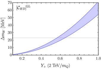
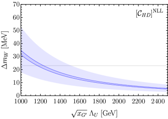
where the WCs are understood to have purely third-family flavor indices. To illustrate the potential importance of this effect, we convert the leading and next-to-leading log contributions to into shifts in (Eq. 128) and plot the result in Fig. 2. One can see for TeV that the NLL running can easily be of the same order or larger than the LL contribution. Additionally, both the LL and NLL contributions to have the same sign and thus add coherently. We include this contribution as well as all NLL running contributions in the couplings and from third-family operators generated at the tree level in the UV in our analysis. The complete expressions for the NLL effects are given in Section B.2, and the proper treatment of the top Yukawa is discussed in detail in Appendix B.
As a final comment, we note that violates custodial symmetry, and therefore its generation should correspond to custodial violations within the model. In the case of the LL contribution, the violation comes from , which is required phenomenologically to pass the bounds on mixing. In the case of the NLL contribution, the custodial symmetry violation is of SM origin, namely . It is interesting to note that taking the symmetric limit in both cases is not possible, so these effects cannot be switched off by invoking custodial symmetry.
III.3 Observables at one-loop accuracy
Besides the tree-level matching and running effects, we include the one-loop matching in , , and of the operators involved in the EW fit, as given in Appendix A. Once this is done, for consistency we have to include the one-loop corrections in of the EWPO. These corrections are of the same size as the non-log-enhanced terms of the one-loop matching. If we include these finite pieces from the one-loop matching, the computation of the EWPO at the tree-level in SMEFT would be basis dependent due to the existence of evanescent operators Fuentes-Martin:2022vvu . However, the one-loop calculation of the observables cancels these ambiguities. Moreover, the IR scale dependence of the observables is also canceled at the leading-log order. For all beyond leading-log effects, we choose to fix . Working in the input scheme Breso-Pla:2021qoe , the EWPO can be written in terms of the and bosons vertex corrections and boson mass shift. In Appendix C we provide all the expressions for these pseudo-observables, including one-loop corrections in .
IV Phenomenology and Global Fit
In the following, we discuss the phenomenology of the model given in Section II featuring third-family quark-lepton unification. We begin with some general remarks about the expected NP effects in EWPO, breaking them down into flavor non-universal and flavor universal effects:
-
•
Flavor non-universal effects. At tree level, the only operators generated by the model that directly affect EWPO are [ and , leading to effects in EW gauge boson couplings to third-family leptons. However, because they are generated with the relation , there is no modification to -boson couplings to tau leptons at tree level. Indeed, only and are affected at tree level, as can be seen in Appendix C. The sign of the effect is such that existing tensions in are worsened, while is made more compatible with data. At the loop level, this statement remains true when considering only LL running in (see Eq. 21), so the leading breaking to the relation comes from LL running effects in the gauge coupling . We give the expressions for this effect in Section B.3 and take it into account in our analysis. However, the effect in is small and we find no significant constraint from it. Similarly, no modification of -boson couplings to bottom quarks is generated at tree level. The leading effect in comes from the breaking of the relation by the -induced running of into (Eq. 19), LL running in , and NLL running in and . These contributions are all of a similar size and we take them into account. Again, we find no significant correction to vertex. There is also a coloron-induced NLL running effect leading to a sizeable modification of the -boson coupling to right-handed bottom quarks (101), but this coupling is poorly constrained and leads to no significant impact on the fit.
-
•
Flavor universal effects. As discussed in detail in Section III.2, LL and NLL running of tree-level operators induced by the new colored states of the model lead to large flavor universal effects in (see Fig. 1). Furthermore, these effects have the same sign and thus add coherently, giving a large universal NP effect that is preferred by the current EW data. In particular, the sign of the effect is such that it increases as well as -pole observables such as , the effective number of neutrinos , and asymmetry observables such as and via flavor universal shifts to the -boson couplings (shown in Appendix C). Finally, the flavor non-universal operator generated at tree level gives flavor-universal contributions to and via LL runnning in . While this effect is irrelevant compared to the universal contribution from , we take it into account via the expressions in Section B.3.
As we will see below, this flavor universal effect in , together with the tree-level non-universal effects in and , are dominantly responsible for the behavior of the EW fit.
We now proceed with a global fit taking into account data from low-energy experiments, EWPO, and neutral current Drell-Yan processes at high-. In principle, the parameters relevant for the phenomenological discussion are:
-
I.
-vector mediated: , , , , , ,
-
II.
Vector-like fermion mediated: , , , , , ,
with and , where , , and are the masses of the heavy 4321 gauge bosons , , and , respectively. Notice that can be written in terms of using Eq. (11), which eliminates it as a free parameter. While is in general a complex parameter, a non-vanishing phase would make it necessary to re-phase the SM fields to match the standard CKM phase convention (see Appendix B of Crosas:2022quq for details). This re-phasing would affect the couplings of the LQ to second-family quarks, namely in Eq. 17. To obtain the correct sign and maximize the effect of the LQ on observables, we fix and consider to be real in what follows. Furthermore, we fix according to the discussion below Eq. 18. As can be seen in Table 4, all tree-level effects are described by the effective scales
| (25) |
up to mass splittings between the 4321 gauge bosons encoded by , . This is no longer true beyond tree level, where the masses appear alone inside logs and loop functions. Still, the leading behavior is captured by the ratios in Eq. 25, so our strategy will be to fix the masses , , , , and to natural values while allowing , , and to vary in the fit freely. The reason we do not fix all masses is that, from Eq. 13, the coupling
| (26) |
is not an independent parameter. Furthermore, we choose to vary instead of since the scale is bounded from below by the process in the EWPO and -decays, so fixing prevents the fit from finding points with very light by fine-tuning the two terms in Eq. 26. The benchmark point for the fixed parameters, and the variables freely varied in the fit, are summarized as follows
-
I.
Fixed parameters: TeV, , , TeV, and TeV ,
-
II.
Varied parameters: , , , , and .
IV.1 Fit Observables and Methodology
We construct the likelihoods used in the fit by building the -function, defined as
| (27) |
where is the inverse of the covariance matrix. Here, we discuss all observables included in the fit and the corresponding theory predictions. The observables we choose to include are:
-
•
LFU tests in transitions. These include the ratios and , as well as , defined as
(28) The expressions for shifts of these observables from their SM predictions in terms of SMEFT operators are given in Appendix D. The world averages of ratios, including the recent LHCb measurement, read HFLAV:2019otj
(29) (30) with correlation . For the SM predictions, we use the HFLAV averages HFLAV:2019otj
(31) Additional discussion about the SM predictions for and their uncertainties can be found in MILC:2015uhg ; Na:2015kha ; Bernlochner:2017jka ; Gambino:2019sif ; Bordone:2019vic ; Martinelli:2021onb . Regarding , we use the recent LHCb measurement as the input LHCb:2022piu and the result in Becirevic:2022bev as the SM prediction
(32) -
•
LFU tests in decays. These are expressed through the ratios
(33) (34) (35) expected to be equal to one in the SM by definition. We use the experimental average from Cornella:2021sby
(36) The theory predictions for the LFU tests can be found in Appendix D.
-
•
Electroweak precision observables. At the - and -pole, we include all the observables listed in Tables 1 and 2 of Ref. Breso-Pla:2021qoe using the same SM theory predictions, and we follow the same input scheme. For the NP theory predictions, we parameterize deviations from the SM due to NP effects via shifts in the and boson couplings, , and the shift in the -boson mass . To simplify notation, we include in the vector and define the theory prediction for a given EWPO as
(37) The theory predictions for the in terms of the SMEFT Wilson coefficients at one-loop in , as well as the map between the EWPO and the that determines the , are given in Appendix C.
We will discuss and compare the fit in the two scenarios, one with and one without the latest CDF II result on CDF:2022hxs . In the former case, given the statistical incompatibility of the CDF II measurement with all the previous determinations, a strategy needs to be defined in order to be able to perform a combination. Our choice is to assume that all experimental errors have been underestimated. Penalizing all measurements “democratically”, and inflating the errors until the per degree of freedom is equal to one, one finds for the averaged mass. Therefore, we consider two scenarios with different input values for
(38) (39) -
•
High- constraints. We consider the tail of distributions obtained at the LHC experiments. The likelihood is obtained using HighPT Allwicher:2022mcg , and for the theory input we use the semi-leptonic SMEFT coefficients computed at NLO in , as discussed in Section A.6. The likelihood is constructed using data from ATLAS ATLAS:2020zms . However, it is interesting to consider also the recent search by CMS CMS:2022goy which shows a small excess, leading to a weaker bound on the NP scale. As done in Ref. Aebischer:2022oqe , we rescale the likelihood obtained from HighPT to match the NLO predictions derived in Ref. Haisch:2022afh for the ATLAS and CMS searches in the b-tag channel. In addition, a lower bound on the vector-like quark mass is implemented by introducing a term in the likelihood of the form
(40) where is the lower bound on the mass at 95% CL CMS:2022fck from direct searches for -doublet vector-like quarks pair-produced via QCD and decaying dominantly to and , as we expect in this model.
IV.2 Fit Results
As discussed in Section IV.1, we have the likelihoods , , , and . We define the global likelihood simply as the sum of the individual likelihoods
| (41) |
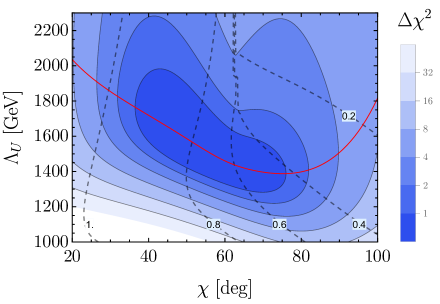
Fixing the parameters as discussed in the beginning of Section IV, the global likelihood is a function of 5-parameters, namely . However, as can be seen in Fig. 3, when choosing the global -function is very flat for , where it changes by less than 2 units along the red line giving the optimal value of . However, the optimal value of (dashed black contours) is not flat in this range. Instead, it decreases from around 1 for to around 0.4 for . Generally speaking, larger values of favor the EWPO which calls for non-zero , while smaller values of favor the observables, which call for larger . Due to the flatness of the -function between and , we choose to fix for everything that follows, to allow for an intermediate value of that strikes a compromise between EWPO and observables while making essentially no difference in the goodness of the fit. We have explicitly checked that this choice for is also good for the fit using .
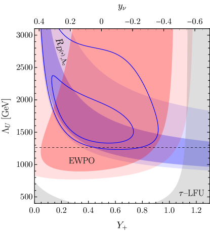
Having fixed the angle , we minimize the global -function with respect to the remaining 4 parameters and report their best-fit values and -confidence intervals in Table 5. The best-fit point (BFP) corresponds to in the case of , indicating a significant improvement over the SM hypothesis.333Assuming 4 degrees of freedom as in Table 5, this change in corresponds to a improvement over the SM hypothesis. However, the effective number of degrees of freedom is likely to be smaller than 4 (and the significance therefore higher) given the poor sensitivity of the fit to some of the free parameters. On the other hand, we note that the selection of observables we have considered is somewhat biased by the choice of the model. Next, we show the and preferred regions in the vs. plane in Fig. 4 for the observables (blue), EWPO (red), as well as the global preferred regions including all observables (blue lines without filling). The region below the dashed black line is excluded by CMS data, while the gray shaded region is excluded by -LFU tests, both at 95% CL. In addition, the explicit relation between the couplings and , fixed by Eq. (26), allows us to show the preferred regions for (upper horizontal axis in Fig. 4) simultaneously. Importantly, the parameters that are not varied in the plots are fixed to their global best-fit points, except in the case of where we fix TeV. This is due to the insensitivity of the fit to when TeV, so we simply choose a theoretically reasonable value in the case. We now offer some general conclusions from the results of the fit.
|
|
 |
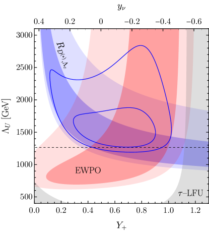 |
In the case of transition observables, we remark that the preferred region allows for larger values as gets smaller. This behavior is mainly dictated by the fact that LFU ratios and receive contributions proportional to , where . Smaller , therefore, increases this contribution, allowing for a higher effective scale to achieve the same size NP effect. Moreover, as shown in Crosas:2022quq , – mixing and measurements of limit the magnitude of , thus requiring larger values of . On the other hand, the confidence interval for translates to . It is very interesting that the results of this fit, which does not include kaon observables, are well compatible with the bound on the leading breaking parameter found in Ref. Crosas:2022quq .
Finally, moving in the direction of larger (smaller ), we observe the simultaneous decrease in the value of necessary to accommodate the data as expected.
Regarding -LFU tests, they exclude at 95% CL for almost all values of , with the bound becoming somewhat stronger for very low values (around 500 GeV) of .
This is due to constructive addition between the tree-level () and one-loop () contributions to the operator (see also the discussion below).
These statements hold where the mass of the right-handed neutrino has been fixed to TeV. At the best-fit point, we have , and the confidence interval is . This corresponds to mixing angles in the range , where GeV. As a consistency check for the fit, these values are well below the bound obtained from EWPO in the literature of Antusch:2014woa ; Antusch:2015mia . Switching on only , we find a similar but somewhat stronger bound of at 95% CL when combining the likelihoods from -LFU tests and EWPO that neatly explains the preferred range on from the fit. We note that smaller values of will lead to a tighter upper bound on , while the bound gets relaxed in the large limit. However, since , it cannot be fully decoupled without simultaneously decoupling the LQ. Therefore, when the scale of the model is low enough to address the charged-current -anomalies, it always predicts sizeable unitarity violations, , in the active neutrino mixing matrix unless is tuned small, as first pointed out in Greljo:2018tuh .
Coming next to the EWPO, one can observe that:
-
i)
When is used as an EWPO (left panel in Fig. 4), the fit generally prefers lower values of and TeV, i.e. those regions in which does not receive a large shift. This is a consequence of the fact that , from the LL contribution to , as can be seen in Eq. 22. Additionally, there is the NLL contribution given in Eq. (24) that is proportional to and adds constructively with the LL contribution. It is interesting that the lower bound of TeV, coming dominantly from the NLL contribution to , is stronger than that of -LFU tests when is fixed to .
-
ii)
When is used as an EWPO (right panel in Fig. 4), the EW fit prefers to have larger , reflected in the fact that larger values of are now preferred by EW precision data for TeV, where the NLL effect is less relevant (as shown in Fig. 2). Furthermore, we note the preferred region also stretches to smaller values of and , and TeV. This is due to the NLL contributions to from the four-quark operators induced by the coloron exchange at tree-level, Eq. 24. This effect is inversely proportional to , and adds constructively with the NLL contribution, allowing a larger mass to be accommodated even for small , provided is small enough.
Finally, we note that for fixed values of the angle , the high- constraints are sensitive only to the value of . The black dashed line gives the 95% CL exclusion limit from CMS, which is providing by far the most stringent lower bound on the NP scale TeV. Similarly, the 95% CL exclusion limit from the ATLAS data is TeV. However, due to the fact that ATLAS currently has an under-fluctuation in the data and is therefore setting more stringent limits than expected (and also does not yet have a dedicated non-resonant search in the channel), we consider the CMS bound of TeV to be the current hard lower bound on the scale. Therefore, in the global fit, we have used the CMS likelihood for . Finally, it is worth mentioning that the right-handed couplings of the LQ to the SM fermions can be reduced in less minimal versions of the model, e.g. via mixing with extra vector-like fermions. In such a case, the bound from high- constraints would be reduced, decreasing the tension with the current ATLAS data Aebischer:2022oqe .
IV.3 Selected Observables
|
|
Having discussed the general behavior of the fit, it is interesting to have a look at the observables that dominantly drive the fit. We define the pull of a particular observable computed in a theoretical model M to be
| (42) |
where is the experimental uncertainty for a given measurement . In Table 6, we show the highest pulling observables for the best-fit point (BFP) of the NP model as well as the same observables within the SM. Furthermore, in Fig. 5 we compare the NP model predictions using (blue regions) with the current experimental determinations for selected individual observables (red regions). We also show the interval for the model parameter being plotted in green, so the overlap of the blue and green regions should be considered as reasonably obtainable within the model. We can make the following observations:
-
•
/ [Figs. 5(a) and 5(b)]. At the best-fit point, we have and , so the model gives a very good fit for , while lying slightly below the central experimental value () for . The reason why a large contribution to can be obtained even for relatively high is due to the right-handed - coupling of the LQ in this model. As the fit prefers , a large constructive scalar contribution to is generated via (see 151). In general, as argued before, smaller values of or are required to increase the contribution to both ratios, which then increases the tension with EWPO or high-, respectively.
-
•
[Figs. 5(c) and 5(d)]. The opposite is true for , where one can see in Fig. 5(c) that larger values of give a larger NP contribution via LL running into . In Fig. 5(d), which shows as a function of , one can see the impact of NLL running into from coloron exchange, giving a large effect in for small values of . The small TeV region is, however, strongly in tension with data. We note that the central value of lies within the overlap of the green and blue regions, and is therefore achievable within the model.
- •
-
•
and -LFU [Figs. 5(g) and 5(h)]. The same flavor non-universal NP effects appear in both observables, predicting in general a decrease from the SM expectation. Also here, the experimental central values lie in opposite directions, with NP effects causing more tension with -LFU measurements. As large corresponds to negative , the asymmetric shape of the prediction for negative values of stems from universal contributions to the -boson couplings to neutrinos via . Such universal shifts cancel out in the LFU ratios and are therefore not seen in Fig. 5(h), where the model always increases the tension with data.
V Conclusions
We have studied for the first time the phenomenological implications of a UV complete model featuring third-family quark-lepton unification for electroweak precision tests. This was done by matching the UV model (defined in Section II) to the SMEFT at one loop, paired with a one-loop computation of the EWPO within the SMEFT (which is necessary to consistently capture all finite parts). We find good agreement between the model predictions for the EWPO and the experimental results, with an overall improvement of the EW fit with respect to the SM.
At tree level, the most sizeable corrections come from integrating out a heavy pseudo-Dirac singlet necessary to account for acceptable neutrino masses within the model. The primary impact of this state on EWPO and -LFU tests is to increase the pre-existing tension in the -boson coupling to third-family leptons. However, one of the most important results of our analysis is the demonstration that higher-order effects play a key role. They give rise to a qualitatively different behavior of the fit compared to the inclusion of tree-level effects only, and break flat directions in the parameter space. In this respect, many of the results we have derived, from the matching to the SMEFT to the computation of EWPO, have a range of applicability that goes well beyond the specific model analyzed here. They provide an important addition to any phenomenological analysis of a wide class of models featuring vector-like fermions, extended gauge groups, or TeV-scale implementations of the inverse-seesaw mechanism.
Concerning the specific framework we have analysed, we find that the new colored states of the model, while not affecting EWPO at the tree level, generate a large flavor universal contribution at the loop level. This loop contribution comes via LL and NLL running, as well as finite one-loop matching contributions to the SMEFT operator . This effect dominates the overall improvement in the electroweak fit via an increase in the -boson mass and universal shifts in several other -pole observables. Furthermore, we observe good compatibility in the interplay of EWPO with other data, such as LFU tests at low energies and high- bounds, where the global best-fit point of the model gives a significant improvement over the SM hypothesis. In the case where the model addresses the charged-current -anomalies, our combined analysis suggests the existence of new states not far above the TeV scale, giving effects in EWPO that cannot be decoupled. This sets a clear target for both current and near-future experiments, both at the intensity and high-energy frontiers.
Acknowledgements
We thank Javier Fuentes Martín and Felix Wilsch for useful discussions in relation to the one-loop matching of the model. This project has received funding from the European Research Council (ERC) under the European Union’s Horizon 2020 research and innovation programme under grant agreement 833280 (FLAY), and by the Swiss National Science Foundation (SNF) under contract 200020-204428.
| (a) | 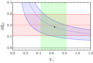 |
(b) | 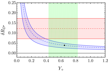 |
| (c) | 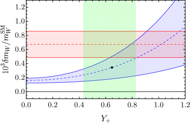 |
(d) | 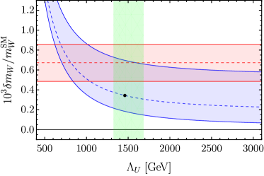 |
| (e) | 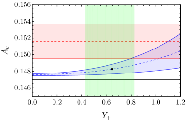 |
(f) | 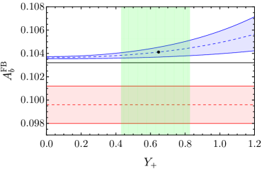 |
| (g) | 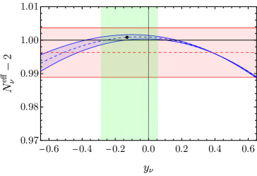 |
(h) | 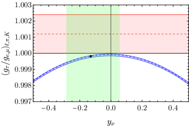 |
Appendix A One-loop matching
A.1 Box-diagram contributions to Higgs-fermion operators
| (a) | (b) | (c) |
The one-loop diagrams in the full theory proceed through box diagrams propagating fermions and either vector or scalar particles, as shown in Fig. 6. In dimensional regularisation with , the box diagram involving a heavy vector of mass , Fig. 6(a), where is the leptoquark mass, reads (omitting the coupling structure and gauge group indices)
| (43) |
with being the external massless spinors whose chirality is projected with , and we defined , with as in Fig. 6. Similarly, in the case of the box diagram with a scalar exchange, Fig. 6(b,c), we distinguish two cases. The first case is when the scalar in question is the massless Higgs boson and the diagram reads
| (44) |
where the same notation, as in the case of a box diagram with the vector exchange, applies. The second case corresponds to the exchange of the Goldstone modes, and since we work in the Feynman gauge, the diagram reads
| (45) |
In the Feynman gauge, the couplings of the Goldstone modes, , to the fermions are Fuentes-Martin:2020hvc
| (46) |
where and , and similarly for leptons. In order to couple to the external Higgs bosons through couplings in Eq. 12, we need a chirality flip on the fermion lines corresponding to the masses and in Fig. 6(c), which reflects in the fact that the amplitude Eq. 45 is proportional to these masses. On the other hand, the couplings of the Goldstone bosons, are
| (47) |
with , and similarly for leptons. Notice that they do not allow for couplings to and . As we are interested in the Higgs-fermion operators with at least one third-generation fermion, we neglect the effects of the and Goldstone bosons.
In the following, we give explicit expressions for the loop functions that appear in the evaluation of Wilson coefficients, written in terms of , , and .
| (48) | |||
| (49) | |||
| (50) |
A.2 Triangle-diagram contributions to Higgs-quark operators
Another type of contribution to the Higgs-fermion operators comes from triangle diagrams as in Fig. 7. At zero momentum, these renormalize the top Yukawa coupling, while the next order in the momenta gives, after applying the equations of motion (EOMs) for the massless external fermions, a contribution to operators.
| (a) | (b) |
Before applying EOMs, these amplitudes match onto three independent structures (operators in the Green’s basis). Following the notation from Gherardi:2020det , these are
| (51) | ||||
| (52) | ||||
| (53) |
The mapping of these onto the Warsaw basis operators reads
| (54) |
where indicate the Wilson coefficients in Green’s basis and we have used . In order to compute the one-loop matching onto and , one needs to choose three different momentum configurations and solve the linear system
| (55) |
where , the matrix encodes the EFT amplitudes, and is determined from the triangle diagrams for different momentum configurations. The final result for the Wilson coefficients is momentum independent, and we can make a convenient choice for the three configurations , such that the result can be written as
| (56) | ||||
| (57) | ||||
| (58) |
where
| (59) |
and
| (60) | ||||
| (61) |
In the following, we give explicit expressions for the loop functions that appear in the evaluation of Wilson coefficients, written in terms of and
| (62) | |||
| (63) |
where we define the function as
| (64) |
A.3 Finite contribution to Higgs-lepton operators from inverse see-saw mechanism
The Yukawa couplings of the Goldstone boson in Eq. 46 give contributions to the Higgs-lepton current operators through the diagrams in Fig. 8.
| (a) | (b) |
Expanding in and keeping only the leading term gives the contribution to dimension-6 operators. Omitting Yukawa couplings, both diagrams give
| (65) |
with
| (66) |
Notice that the Yukawa coupling involving in Eq. 46 is proportional to , so the dependence on will cancel. Adding the two diagrams we get contributions to and .
A.4 Results: finite parts
In the following, we will present the results for the finite parts of the Wilson coefficients from the one-loop matching procedure. In the previous sections, we have shown the contributions in the full UV theory. In order to obtain the matching, both tree-level and one-loop contributions in the SMEFT must be taken into account.
| (a) | (b) | (c) | (d) |
| (a) | (b) |
A.5 Matching of
| (a) | (b) | (c) |
The relevant diagrams for the matching of , both in the SMEFT and in the full 4321 model, are shown in Fig. 11. Similarly to the case of the triangle diagrams above, the four-point function receives contributions from four operators in the Green’s basis Gherardi:2020det :
| (71) | ||||
| (72) | ||||
| (73) | ||||
| (74) |
Therefore, we need to choose four different momentum configurations for the external Higgs states, , and , set up the system for , and , and solve for . We obtain
| (75) |
with the loop functions being
| (76) | ||||
| (77) |
and .
A.6 Semileptonic Wilson coefficients at one loop
The relevant four-fermion Wilson coefficients for transitions and high-, improved with the NLO corrections in gauge coupling, where , read
| (78) | ||||
| (79) | ||||
| (80) | ||||
| (81) | ||||
| (82) | ||||
| (83) | ||||
| (84) | ||||
| (85) |
where the loop functions are
| (86) | ||||
| (87) | ||||
| (88) | ||||
| (89) | ||||
| (90) |
In the limit of vanishing vector-like fermion masses, , the loop functions go to 1, while , thus reproducing the results of Ref. Fuentes-Martin:2019ign ; Fuentes-Martin:2020luw .
Appendix B Running effects
We include the running of the Wilson coefficients from the UV to the EW scale. This running can be found solving the RGE equations:
| (91) |
where is a vector with all dimension 6 Wilson coefficients, including flavor indices, and is the anomalous dimension matrix, that can be read from Jenkins:2013zja ; Jenkins:2013wua ; Alonso:2013hga :
| (92) |
The anomalous dimension matrix depends on through the running of the SM parameters. Notice that the impact of dimension 6 operators on the SM parameters running is a dimension 8 effect Fuentes-Martin:2020zaz so it can be neglected. The solution to this differential equation is
| (93) |
where is the -ordered product. If we neglect the running of the SM parameters, Eq. 93 reads
| (94) |
B.1 Leading-log running in
The one-integral term of the expansion in Eq. 93 corresponds to the leading-log running. In this work, the most important leading-log contribution to the operators relevant for the EW fit is the one induced by the top Yukawa ( does not induce any leading-log running in the sector relevant for our model):
| (95) |
where is the average of ,
| (96) |
Substituting , we recover the leading-log formulas given in section III.2.1. Running from TeV to , and using DsixTools Fuentes-Martin:2020zaz , we get , which is the value we use for in this work.
B.2 Next-to-leading-log running in and
The two-integral term of (93), or the term of (94), give the next-to-leading-log running. Including and effects, using the tree-level expressions of the third-family Wilson coefficients of Table 3, and running from the UV, we get:
| (97) | ||||
| (98) | ||||
| (99) | ||||
| (100) | ||||
| (101) |
These expressions include the running of the SM parameters if for we use the average of Eq. 96, and for , the average
| (102) |
Running from TeV to , and using DsixTools Fuentes-Martin:2020zaz , we get .
B.3 Leading-log running in
The weak running in gives contributions to and , but not to the corresponding singlet Wilson coefficients. Taking the leading log, neglecting the running of , and using that is real, we find that the third-family contributions are
| (103) |
Similarly, using that is real, we find
| (104) |
where the sum on is understood to be over the and contributions to . In terms of the model parameters, the Wilson coefficients read
| (105) |
and similarly
| (106) |
Appendix C Electroweak observables at 1-loop
C.1 Connection with SMEFT
Inserting the generated SMEFT operators induces vertex and mass modifications of the EW gauge bosons. Working in the input scheme, the relevant terms of the effective Lagrangian for the EW fit become Breso-Pla:2021qoe
| (107) |
where
| (108) |
The vertex modifications of the -boson are
| (109) | ||||
| (110) | ||||
| (111) | ||||
| (112) | ||||
| (113) | ||||
| (114) | ||||
| (115) |
where is a family-universal contribution that is given by
| (116) |
| (a) | (b) | (c) |
To be consistent with the one-loop matching, we include one-loop corrections in . In our model, they are given by the diagrams in Fig. 12. Notice that neglecting terms and , diagrams (a) and (b) only affect the purely third-family vertices. In principle, diagram (c) affects the -mass, but due to the input scheme we are using this correction is translated into a correction of the flavor-universal shift and the -mass we show below. The one-loop corrections in to the -vertex modifications relevant for the EW fit (which excludes the coupling) in our model are
| (117) | ||||
| (118) | ||||
| (119) | ||||
| (120) | ||||
| (121) | ||||
| (122) | ||||
| (123) | ||||
| (124) |
Notice that in Eq. 114 is only sensitive to the sum of and . This sum contains finite pieces of the one-loop matching given in Sections A.4 and A.4,
| (125) |
If we neglect the running, these finite pieces exactly cancel with the non-log terms of the one-loop correction to in Eq. 123. Moreover, when we insert the four-fermion operators at the tree level (see Table 3) in the one-loop corrections to all vertex modifications relevant for the EW fit, and contributions systematically cancel, leaving only the leptoquark contributions.
The variations of the couplings relevant for the EW fit (which excludes the vertex), including the one-loop corrections in (diagram (b) of Fig. 12) are
| (126) | ||||
| (127) |
The mass modification, including the one-loop corrections in our model, is
| (128) |
C.2 Electroweak observable variations
To construct the likelihood for the EW fit, we use the observables of Tables 1 and 2 of Breso-Pla:2021qoe , that collect the measurements presented in ALEPH:2005ab ; Janot:2019oyi ; dEnterria:2020cgt ; SLD:2000jop ; ParticleDataGroup:2020ssz ; ALEPH:2013dgf ; CDF:2005bdv ; LHCb:2016zpq ; ATLAS:2016nqi ; D0:1999bqi ; ATLAS:2020xea , and the SM predictions. Some sub-blocks of the observables are correlated. In Table 7 and Table 8 we provide the correlations among these sub-blocks for the -pole observables ALEPH:2005ab and the -pole observables ALEPH:2013dgf respectively.
| 1 | 0.105 | 0.131 | 0.092 | 0.001 | 0.003 | 0.002 | |
| 1 | 0.069 | 0.046 | -0.371 | 0.02 | 0.013 | ||
| 1 | 0.069 | 0.001 | 0.012 | -0.003 | |||
| 1 | 0.003 | 0.001 | 0.009 | ||||
| 1 | -0.024 | -0.02 | |||||
| 1 | 0.046 | ||||||
| 1 |
| 1 | -0.18 | -0.1 | 0.07 | |
| 1 | 0.04 | -0.06 | ||
| 1 | 0.15 | |||
| 1 |
| 1 | 0.038 | 0.033 | |
| 1 | 0.007 | ||
| 1 |
| 1 | 0.11 | |
| 1 |
| Br | Br | Br | |
|---|---|---|---|
| Br | 1 | 0.136 | -0.201 |
| Br | 1 | -0.122 | |
| Br | 1 |
We calculate the variation of the observables, , at leading order in the EW boson vertex modifications and , as defined in Eq. 107, and neglecting the SM fermion masses. The expressions of the EW boson vertex modifications and in terms of the SMEFT Wilson coefficients are given in Section C.1. To write the variation of the observables, it is convenient first to define
| (129) | ||||
| (130) | ||||
| (131) | ||||
| (132) | ||||
| (133) | ||||
| (134) | ||||
| (135) |
where represents the SM prediction of the observable at the tree level. The variation of the -pole observables is then
| (136) | ||||
| (137) | ||||
| (138) | ||||
| (139) | ||||
| (140) | ||||
| (141) | ||||
| (142) | ||||
| (143) |
The variation of the -pole observables, working in the limit , is
| (144) | ||||
| (145) | ||||
| (146) | ||||
| (147) |
where , and . The effective number of neutrinos describes the invisible width,
| (148) |
It is not an observable of the EW fit itself, but can be calculated as a function of some of the EWPO ALEPH:2005ab ; Janot:2019oyi . Its variation, as function of the -vertex modifications is
| (149) |
Appendix D Expressions for other observables
D.1 transitions
The Lagrangian relevant for transitions affecting the LFU ratios , is
| (150) |
so the LFU ratios read
| (151) | ||||
| (152) | ||||
| (153) |
The running can be neglected for , but not for . Including QCD running effects,
| (154) |
Defining the following Wilson coefficients
| (155) |
the mapping to the Warsaw basis is
| (156) | ||||
| (157) |
D.2 LFU ratios
Following Allwicher:2021ndi , the LFU ratios can be expressed in terms of SMEFT coefficients as
| (158) |
where we have used the assumption that only couplings to taus are affected and substituted the tree-level matching for the as in Table 4.
References
- (1) M. Bordone, C. Cornella, J. Fuentes-Martin and G. Isidori, A three-site gauge model for flavor hierarchies and flavor anomalies, Phys. Lett. B 779 (2018) 317–323, [1712.01368].
- (2) A. Greljo and B. A. Stefanek, Third family quark–lepton unification at the TeV scale, Phys. Lett. B 782 (2018) 131–138, [1802.04274].
- (3) J. Fuentes-Martin, G. Isidori, J. Pagès and B. A. Stefanek, Flavor non-universal Pati-Salam unification and neutrino masses, Phys. Lett. B 820 (2021) 136484, [2012.10492].
- (4) J. Fuentes-Martín and P. Stangl, Third-family quark-lepton unification with a fundamental composite Higgs, Phys. Lett. B 811 (2020) 135953, [2004.11376].
- (5) J. Fuentes-Martin, G. Isidori, J. M. Lizana, N. Selimovic and B. A. Stefanek, Flavor hierarchies, flavor anomalies, and Higgs mass from a warped extra dimension, Phys. Lett. B 834 (2022) 137382, [2203.01952].
- (6) J. Davighi, G. Isidori and M. Pesut, Electroweak-flavour and quark-lepton unification: a family non-universal path, 2212.06163.
- (7) G. R. Dvali and M. A. Shifman, Families as neighbors in extra dimension, Phys. Lett. B 475 (2000) 295–302, [hep-ph/0001072].
- (8) G. Panico and A. Pomarol, Flavor hierarchies from dynamical scales, JHEP 07 (2016) 097, [1603.06609].
- (9) L. Allwicher, G. Isidori and A. E. Thomsen, Stability of the Higgs Sector in a Flavor-Inspired Multi-Scale Model, JHEP 01 (2021) 191, [2011.01946].
- (10) R. Barbieri, A View of Flavour Physics in 2021, Acta Phys. Polon. B 52 (2021) 789, [2103.15635].
- (11) L. Di Luzio, A. Greljo and M. Nardecchia, Gauge leptoquark as the origin of B-physics anomalies, Phys. Rev. D 96 (2017) 115011, [1708.08450].
- (12) J. C. Pati and A. Salam, Lepton Number as the Fourth Color, Phys. Rev. D 10 (1974) 275–289.
- (13) R. Alonso, B. Grinstein and J. Martin Camalich, Lepton universality violation and lepton flavor conservation in -meson decays, JHEP 10 (2015) 184, [1505.05164].
- (14) L. Calibbi, A. Crivellin and T. Ota, Effective Field Theory Approach to , and with Third Generation Couplings, Phys. Rev. Lett. 115 (2015) 181801, [1506.02661].
- (15) R. Barbieri, G. Isidori, A. Pattori and F. Senia, Anomalies in -decays and flavour symmetry, Eur. Phys. J. C 76 (2016) 67, [1512.01560].
- (16) B. Bhattacharya, A. Datta, J.-P. Guévin, D. London and R. Watanabe, Simultaneous Explanation of the and Puzzles: a Model Analysis, JHEP 01 (2017) 015, [1609.09078].
- (17) D. Buttazzo, A. Greljo, G. Isidori and D. Marzocca, B-physics anomalies: a guide to combined explanations, JHEP 11 (2017) 044, [1706.07808].
- (18) BaBar collaboration, J. P. Lees et al., Measurement of an Excess of Decays and Implications for Charged Higgs Bosons, Phys. Rev. D 88 (2013) 072012, [1303.0571].
- (19) Belle collaboration, S. Hirose et al., Measurement of the lepton polarization and in the decay , Phys. Rev. Lett. 118 (2017) 211801, [1612.00529].
- (20) LHCb collaboration, R. Aaij et al., Measurement of the ratio of branching fractions , Phys. Rev. Lett. 115 (2015) 111803, [1506.08614].
- (21) LHCb collaboration, R. Aaij et al., Measurement of the ratio of the and branching fractions using three-prong -lepton decays, Phys. Rev. Lett. 120 (2018) 171802, [1708.08856].
- (22) LHCb collaboration, R. Aaij et al., Test of Lepton Flavor Universality by the measurement of the branching fraction using three-prong decays, Phys. Rev. D 97 (2018) 072013, [1711.02505].
- (23) LHCb collaboration, Test of lepton universality in decays, 2212.09152.
- (24) L. Allwicher, G. Isidori and N. Selimovic, LFU violations in leptonic decays and B-physics anomalies, Phys. Lett. B 826 (2022) 136903, [2109.03833].
- (25) L. Di Luzio, J. Fuentes-Martin, A. Greljo, M. Nardecchia and S. Renner, Maximal Flavour Violation: a Cabibbo mechanism for leptoquarks, JHEP 11 (2018) 081, [1808.00942].
- (26) J. Fuentes-Martín, G. Isidori, M. König and N. Selimović, Vector Leptoquarks Beyond Tree Level III: Vector-like Fermions and Flavor-Changing Transitions, Phys. Rev. D 102 (2020) 115015, [2009.11296].
- (27) O. L. Crosas, G. Isidori, J. M. Lizana, N. Selimovic and B. A. Stefanek, Flavor non-universal vector leptoquark imprints in and transitions, Phys. Lett. B 835 (2022) 137525, [2207.00018].
- (28) L. Allwicher, D. A. Faroughy, F. Jaffredo, O. Sumensari and F. Wilsch, Drell-Yan Tails Beyond the Standard Model, 2207.10714.
- (29) M. J. Baker, J. Fuentes-Martín, G. Isidori and M. König, High- signatures in vector–leptoquark models, Eur. Phys. J. C 79 (2019) 334, [1901.10480].
- (30) L. Buonocore, U. Haisch, P. Nason, F. Tramontano and G. Zanderighi, Lepton-Quark Collisions at the Large Hadron Collider, Phys. Rev. Lett. 125 (2020) 231804, [2005.06475].
- (31) L. Buonocore, A. Greljo, P. Krack, P. Nason, N. Selimović, F. Tramontano et al., Resonant leptoquark at NLO with POWHEG, JHEP 11 (2022) 129, [2209.02599].
- (32) F. Feruglio, P. Paradisi and A. Pattori, Revisiting Lepton Flavor Universality in B Decays, Phys. Rev. Lett. 118 (2017) 011801, [1606.00524].
- (33) F. Feruglio, P. Paradisi and A. Pattori, On the Importance of Electroweak Corrections for B Anomalies, JHEP 09 (2017) 061, [1705.00929].
- (34) E. E. Jenkins, A. V. Manohar and M. Trott, Renormalization Group Evolution of the Standard Model Dimension Six Operators I: Formalism and lambda Dependence, JHEP 10 (2013) 087, [1308.2627].
- (35) E. E. Jenkins, A. V. Manohar and M. Trott, Renormalization Group Evolution of the Standard Model Dimension Six Operators II: Yukawa Dependence, JHEP 01 (2014) 035, [1310.4838].
- (36) R. Alonso, E. E. Jenkins, A. V. Manohar and M. Trott, Renormalization Group Evolution of the Standard Model Dimension Six Operators III: Gauge Coupling Dependence and Phenomenology, JHEP 04 (2014) 159, [1312.2014].
- (37) J. Fuentes-Martín, M. König, J. Pagès, A. E. Thomsen and F. Wilsch, Evanescent operators in one-loop matching computations, JHEP 02 (2023) 031, [2211.09144].
- (38) V. Bresó-Pla, A. Falkowski and M. González-Alonso, AFB in the SMEFT: precision Z physics at the LHC, JHEP 08 (2021) 021, [2103.12074].
- (39) HFLAV [https://hflav.web.cern.ch] collaboration, Y. S. Amhis et al., Averages of b-hadron, c-hadron, and -lepton properties as of 2018, Eur. Phys. J. C 81 (2021) 226, [1909.12524].
- (40) MILC collaboration, J. A. Bailey et al., B→D form factors at nonzero recoil and —Vcb— from 2+1-flavor lattice QCD, Phys. Rev. D 92 (2015) 034506, [1503.07237].
- (41) HPQCD collaboration, H. Na, C. M. Bouchard, G. P. Lepage, C. Monahan and J. Shigemitsu, form factors at nonzero recoil and extraction of , Phys. Rev. D 92 (2015) 054510, [1505.03925].
- (42) F. U. Bernlochner, Z. Ligeti, M. Papucci and D. J. Robinson, Combined analysis of semileptonic decays to and : , , and new physics, Phys. Rev. D 95 (2017) 115008, [1703.05330].
- (43) P. Gambino, M. Jung and S. Schacht, The puzzle: An update, Phys. Lett. B 795 (2019) 386–390, [1905.08209].
- (44) M. Bordone, M. Jung and D. van Dyk, Theory determination of form factors at , Eur. Phys. J. C 80 (2020) 74, [1908.09398].
- (45) G. Martinelli, S. Simula and L. Vittorio, and ) using lattice QCD and unitarity, Phys. Rev. D 105 (2022) 034503, [2105.08674].
- (46) LHCb collaboration, R. Aaij et al., Observation of the decay , Phys. Rev. Lett. 128 (2022) 191803, [2201.03497].
- (47) D. Bečirević and F. Jaffredo, Looking for the effects of New Physics in the decay mode, 2209.13409.
- (48) C. Cornella, D. A. Faroughy, J. Fuentes-Martin, G. Isidori and M. Neubert, Reading the footprints of the B-meson flavor anomalies, JHEP 08 (2021) 050, [2103.16558].
- (49) CDF collaboration, T. Aaltonen et al., High-precision measurement of the boson mass with the CDF II detector, Science 376 (2022) 170–176.
- (50) L. Allwicher, D. A. Faroughy, F. Jaffredo, O. Sumensari and F. Wilsch, HighPT: A Tool for high- Drell-Yan Tails Beyond the Standard Model, 2207.10756.
- (51) ATLAS collaboration, G. Aad et al., Search for heavy Higgs bosons decaying into two tau leptons with the ATLAS detector using collisions at TeV, Phys. Rev. Lett. 125 (2020) 051801, [2002.12223].
- (52) CMS collaboration, Searches for additional Higgs bosons and for vector leptoquarks in final states in proton-proton collisions at = 13 TeV, 2208.02717.
- (53) J. Aebischer, G. Isidori, M. Pesut, B. A. Stefanek and F. Wilsch, Confronting the vector leptoquark hypothesis with new low- and high-energy data, 2210.13422.
- (54) U. Haisch, L. Schnell and S. Schulte, Drell-Yan production in third-generation gauge vector leptoquark models at NLO+PS in QCD, 2209.12780.
- (55) CMS collaboration, Search for pair production of vector-like quarks in leptonic final states in proton-proton collisions at = 13 TeV, 2209.07327.
- (56) S. Antusch and O. Fischer, Non-unitarity of the leptonic mixing matrix: Present bounds and future sensitivities, JHEP 10 (2014) 094, [1407.6607].
- (57) S. Antusch and O. Fischer, Testing sterile neutrino extensions of the Standard Model at future lepton colliders, JHEP 05 (2015) 053, [1502.05915].
- (58) V. Gherardi, D. Marzocca and E. Venturini, Matching scalar leptoquarks to the SMEFT at one loop, JHEP 07 (2020) 225, [2003.12525].
- (59) J. Fuentes-Martín, G. Isidori, M. König and N. Selimović, Vector Leptoquarks Beyond Tree Level, Phys. Rev. D 101 (2020) 035024, [1910.13474].
- (60) J. Fuentes-Martín, G. Isidori, M. König and N. Selimović, Vector leptoquarks beyond tree level. II. corrections and radial modes, Phys. Rev. D 102 (2020) 035021, [2006.16250].
- (61) J. Fuentes-Martin, P. Ruiz-Femenia, A. Vicente and J. Virto, DsixTools 2.0: The Effective Field Theory Toolkit, Eur. Phys. J. C 81 (2021) 167, [2010.16341].
- (62) ALEPH, DELPHI, L3, OPAL, SLD, LEP Electroweak Working Group, SLD Electroweak Group, SLD Heavy Flavour Group collaboration, S. Schael et al., Precision electroweak measurements on the resonance, Phys. Rept. 427 (2006) 257–454, [hep-ex/0509008].
- (63) P. Janot and S. Jadach, Improved Bhabha cross section at LEP and the number of light neutrino species, Phys. Lett. B 803 (2020) 135319, [1912.02067].
- (64) D. d’Enterria and C. Yan, Revised QCD effects on the Z forward-backward asymmetry, 2011.00530.
- (65) SLD collaboration, K. Abe et al., First direct measurement of the parity violating coupling of the Z0 to the s quark, Phys. Rev. Lett. 85 (2000) 5059–5063, [hep-ex/0006019].
- (66) Particle Data Group collaboration, P. A. Zyla et al., Review of Particle Physics, PTEP 2020 (2020) 083C01.
- (67) ALEPH, DELPHI, L3, OPAL, LEP Electroweak collaboration, S. Schael et al., Electroweak Measurements in Electron-Positron Collisions at W-Boson-Pair Energies at LEP, Phys. Rept. 532 (2013) 119–244, [1302.3415].
- (68) CDF collaboration, A. Abulencia et al., Measurements of inclusive W and Z cross sections in p anti-p collisions at s**(1/2) = 1.96-TeV, J. Phys. G 34 (2007) 2457–2544, [hep-ex/0508029].
- (69) LHCb collaboration, R. Aaij et al., Measurement of forward production in collisions at TeV, JHEP 10 (2016) 030, [1608.01484].
- (70) ATLAS collaboration, M. Aaboud et al., Precision measurement and interpretation of inclusive , and production cross sections with the ATLAS detector, Eur. Phys. J. C 77 367, [1612.03016].
- (71) D0 collaboration, B. Abbott et al., A measurement of the production cross section in collisions at TeV, Phys. Rev. Lett. 84 (2000) 5710–5715, [hep-ex/9912065].
- (72) ATLAS collaboration, G. Aad et al., Test of the universality of and lepton couplings in -boson decays with the ATLAS detector, Nature Phys. 17 (2021) 813–818, [2007.14040].