Approximation Ineffectiveness of a Tour-Untangling Heuristic

Abstract

We analyze a tour-uncrossing heuristic for the Euclidean Travelling Salesperson Problem, showing that its worst-case approximation ratio is $\Omega(n)$ and its average-case approximation ratio is $\Omega(\sqrt{n})$ in expectation. We furthermore evaluate the approximation performance of this heuristic numerically on average-case instances, and find that it performs far better than the average-case lower bound suggests. This indicates a shortcoming in the approach we use for our analysis, which is a rather common method in the analysis of local search heuristics.

1 Introduction

The Travelling Salesperson Problem (TSP) is a classic example of an NP-hard combinatorial optimization problem [8]. Different variants of the problem exist, with one of the most studied variants being the Euclidean TSP. In this version, the weight of an edge is given by the Euclidean distance between its endpoints. Even this restricted version is NP-hard [9].

Due to this hardness, practitioners often turn to approximation algorithms and heuristics for the TSP. One simple heuristic is 2-opt [1]. In each iteration of this heuristic, one searches for a pair of edges in the tour that can be replaced by a different pair, such that the total length of the tour decreases. Although this heuristic performs quite well in practice [1, Chapter 8], it may require an exponential number of iterations to converge even in the plane [6].

Interestingly, Van Leeuwen & Schoone showed that a restricted variant of 2-opt in which one only removes intersecting edges terminates in $O(n^{3})$ iterations in the worst case [11]. For convenience, we refer to this variant as X-opt. More recently, da Fonseca et al. [5] analyzed this heuristic once more, extending the results to matching problems and showing a bound of $O(tn^{2})$ for instances where all but $t$ points are in convex position. Their work builds on previous related work on computing uncrossing matchings [2].

The insight that removing intersecting edges improves the tour is a key intuition behind 2-opt. However, not all 2-opt iterations remove intersections. Indeed, 2-opt has proved extremely effective also for non-metric TSP instances, where there is no notion of intersecting edges at all.

This raises the question of approximation performance: can one get away with using X-opt instead of 2-opt at minimal cost to the approximation guarantee, thereby ensuring an efficient heuristic for TSP instances in the plane? The approximation ratio of 2-opt has long been known to sit between $\Omega\mathopen{}\mathclose{{}\left(\frac{\log n}{\log\log n}}\right)$ and $O(\log n)$ for $d$-dimensional Euclidean instances [4], and has recently been settled to $\Theta\mathopen{}\mathclose{{}\left(\frac{\log n}{\log\log n}}\right)$ for 2-dimensional instances [3]. However, no previous work seems to have discussed X-opt.

We analyze this simpler case here, showing an approximation ratio of $\Omega(n)$ in the worst case and $\Omega(\sqrt{n})$ in the average case. This answers our previously raised question in the negative; in order to obtain a good approximation ratio, one must allow for iterations that improve the tour without removing intersections. Especially the average-case result stands in stark contrast to the average-case approximation ratio of 2-opt, which is known to be $O(1)$ [4].

We also perform a numerical experiment, which presents a different picture from our formal results. To within the precision we are able to achieve, our experiments indicate an average-case approximation ratio of X-opt of $O(1)$. We consider this evidence that the techniques we use to obtain the average-case bound of $\Omega(\sqrt{n})$, which are standard techniques used to perform probabilistic analyses of local search heuristics, fall short of explaining the true practical performance of X-opt.

1.1 Definitions and Notation

Given two points $x,y\in\mathbb{R}^{2}$, we define $d(x,y)$ as the Euclidean distance between $x$ and $y$. We define $L(x,y)$ as the line segment between $x$ and $y$. By an abuse of notation, if $e=\{x,y\}$ with $x\neq y$, we write $L(e)=L(x,y)$. We write $\ell(e)=d(x,y)$ for the length of $L(e)$.

Let $X\subseteq\mathbb{R}^{2}$. For a set $E\subseteq\{e\in 2^{X}\>\lvert\>|e|=2\}$, we write $\ell(E)=\sum_{e\in E}\ell(e)$. If $L(e)\cap L(f)\neq\emptyset$ for some $e,f\in E$, i.e., some of the line segments represented by the edges in $E$ intersect, then we say $E$ is crossing. Conversely, if $E$ is not crossing, then it is noncrossing. In particular, a local optimum for X-opt is exactly a noncrossing tour.

Given $A\subset\mathbb{R}^{2}$ and $x\in\mathbb{R}^{2}$, we define the distance between $A$ and $x$ as $d(x,A)=\min_{y\in A}d(x,y)$. Note that $d(x,A)$ might not exist, for instance, if $A$ is an open set. However, we will only consider sets for which $d(x,A)$ is well-defined.

Let $A$ be a rectangular region in $\mathbb{R}^{2}$. Let $X$ be a set of $n$ points in $A$. We call the four line segments that make up the boundary of $A$ the edges of $A$. For an edge $e$ of $A$, let $x_{e}=\arg\min_{x\in X}d(x,e)$ be the point closest to $e$. We call $X$ nice for $A$ if for each pair of edges $e$, $f$ of $A$, it holds that $x_{e}\neq x_{f}$.

Figure 1: The construction used in Theorem 2.1. Left: a noncrossing tour of length $\Omega(n)$. Right: a tour of length $O(1)$.

2 Worst Case

We construct a worst-case instance in which there exists a noncrossing tour with length $\Omega(n)$, as well as a tour of constant length. The construction we use is depicted in Figure 1.

Theorem 2.1

Let $n\in\mathbb{N}$ be even. For $\epsilon>0$ sufficiently small, there exists an instance of the Euclidean TSP in the plane where X-opt has approximation ratio at least $\frac{n}{2}\cdot(1-\epsilon)$. In particular, the approximation ratio can be brought arbitrarily close to $\frac{n}{2}$.

Proof

We place one point $s$ at $(0,0)$. Next, we place $k=n/2$ points equally spaced along the line segment extending from $(1-\epsilon/2,1)$ to $(1,1-\epsilon/2)$. We label these points $\{y_{i}\}_{i=1}^{k}$, ordering them by increasing $x$-coordinate.

Consider the cone $K$ with vertex at the origin, defined by all conic combinations of $\{y_{1},y_{k}\}$. Define the height along the axis of $K$ of a point $a$ by the distance of $a$ from the origin along the axis of $K$. We place $k-1$ points along the line segment perpendicular to the axis of $K$ at a height $\epsilon/\sqrt{8}$, excluding its endpoints. We label these points $\{x_{i}\}_{i=1}^{k-1}$, sorting them again by increasing $x$-coordinate. Note that it does not matter where exactly we place these points, as long as no two points are placed in the same location. Observe that we have now placed exactly $2k=n$ points inside $[0,1]^{2}$.

To draw a noncrossing tour, we start at $s$, and draw the edge $\{s,y_{1}\}$. We then draw the edges $\{y_{i},x_{i}\}_{i=1}^{k-1}$. Lastly, we add the edges $\{x_{k-1},y_{k}\}$ and $\{y_{k},s\}$, which closes up the tour.

By construction, this tour contains no intersecting edges. To bound its length from below, observe that all edges have a length of at least $\sqrt{2}-\epsilon/\sqrt{2}=\sqrt{2}(1-\epsilon/2)$. Thus, this tour has a length of at least $\sqrt{2}n(1-\epsilon/2)$.

We now bound the length of the optimal tour from above, by

$$d(s,x_{1})+d(x_{1},y_{1})+d(s,x_{k-1})+d(x_{k-1},y_{k})+d(x_{1},x_{k})+d(y_{1},y_{k})\leq 2\sqrt{2}(1+\epsilon/2).$$

Putting these bounds together, we find a ratio of

$$\frac{\sqrt{2}n(1-\epsilon/2)}{2\sqrt{2}(1+\epsilon/2)}=\frac{n}{2}\cdot\frac{1-\epsilon/2}{1+\epsilon/2}\geq\frac{n}{2}\cdot(1-\epsilon),$$

as claimed. ∎

Remark

The construction used for Theorem 2.1 only holds for $n$ even. For odd $n$, we can use a similar construction, but the approximation ratio then becomes $(n-1)/2\cdot(1-\epsilon)$.

A simple argument shows that the approximation ratio given in Theorem 2.1 is essentially as bad as one can get in the metric TSP. Given any instance, let $x$ and $y$ be those points separated by the greatest distance. Any tour must travel from $x$ to $y$ and back to $x$ again, so any tour is of length at least $2\cdot d(x,y)$. Moreover, every tour contains exactly $n$ edges, so any tour has length at most $n\cdot d(x,y)$. Hence, the approximation ratio of any algorithm for the metric TSP is at most $n/2$.

3 Average Case

Although the worst-case construction of Section 2 shows that the uncrossing heuristic may yield almost as bad of an approximation as is possible for TSP, it is possible that the heuristic still shows good behavior on average. To exclude this possibility, we consider a standard average-case model wherein $n$ points are placed uniformly and independently in the plane. We then construct a tour of length $\Omega(n)$ in expectation. We present our results in Theorem 3.3.

To simplify our arguments, it would be convenient if we could consider only a subset of all points, so that we can look at a linear-size sub-instance with nicer properties. Constructing a long noncrossing tour through this subset would be much easier.

Since an optimal tour through a set of points $X$ is always at least as long as an optimal tour through a subset $Y\subset X$, it is tempting to conjecture that something similar holds for all noncrossing tours. Perhaps, given a noncrossing tour through $Y\subseteq X$, we can extend the tour to all of $X$ without decreasing its length?

Unfortunately, this turns out to be false. We provide a counterexample in Figure 2.

Figure 2: Left: instance described in Theorem 3.1. Center: the tour $T$ from Theorem 3.1. Right: the longest possible noncrossing tour through all points in the instance.

Theorem 3.1

There exists a set of points in the plane, together with a noncrossing tour $T$ through all but one of these points, such that all noncrossing tours through all points have length strictly less than $\ell(T)$.

Proof

Consider the instance shown in Figure 2, along with the tour $T=avcubwa$. Note that $T$ passes through all points, except for the central point $x$. We construct this instance such that $d(b,c)=d(a,b)=d(a,c)=1$, so that $a$, $b$ and $c$ form the vertices of an equilateral triangle. We also set the distances $d(v,c)=d(b,u)=d(a,w)=L$, where $L\gg 1$. We set the angle $\angle cub=\angle avc=\angle awb$ small, so that $d(c,u)=d(v,a)=d(b,w)=L-1+o(1)$; here, $o(1)$ means terms decreasing in $L$. For instance, setting this angle to $1/L$ would suffice. Then we have $d(w,c)=L-\frac{1}{2}+o(1)$. By construction, $d(x,a)=d(x,b)=d(x,c)=1/\sqrt{3}$. We can furthermore compute $d(u,v)=d(v,w)=d(u,w)=\sqrt{3}L+o(1)$, $d(a,u)=d(b,v)=d(c,w)=L-\frac{1}{2}+o(1)$, and $d(x,u)=d(x,v)=d(x,w)=L-\frac{1}{4\sqrt{3}}+o(1)$. Since we will compare sums of these various distances, all inequalities in the remainder of the proof are understood to hold for sufficiently large $L$.

We classify the edges into types:

Type	1	2	3	4	5	6	7
Length (up to $o(1)$ terms)	$\frac{1}{\sqrt{3}}$	1	$L-1$	$L-\frac{1}{2}$	$L-\frac{1}{4\sqrt{3}}$	$L$	$\sqrt{3}L$

We furthermore call the edges of types 1 and 2 the short edges, of types 3 through 6 the long edges, and of type 7 the very long edges. Finally, we classify the points $\{a,b,c,u,v,w\}$ into the near points $N=\{a,b,c\}$ and the far points $F=\{u,v,w\}$.

We start by computing the length of $T$:

$$\ell(T)=3L+3(L-1)+o(1)=6L-3+o(1).$$

We now show that all noncrossing tours that include $x$ are shorter than $6L-3+o(1)$.

As it is laborious to check all possible noncrossing tours, we begin by excluding some possibilities. First, suppose the tour contains $k$ very long edges. Then the tour can contain at most $6-2k$ long edges, since each long edge has exactly one endpoint in $F$, and $k+1$ of these have been used. Such a tour has a length of at most $k\sqrt{3}+(6-2k)L+O(1)<6L-3+o(1)$. Thus, any sufficiently long tour cannot contain any very long edges.

Now suppose that a tour contains two short edges. Since very long edges are excluded, such a tour has length at most $5L+2+o(1)<6L-3+o(1)$. Therefore, the tour must consist of six long edges and one short edge.

Suppose the unique short edge in our tour is of type 2. Without loss of generality, we assume it is $\{a,b\}$. Since all other edges are long, both $a$ and $b$ must connect to points in $F$. Suppose $a$ connects to $u$. Then $x$ must connect to $u$ and $w$, since otherwise we would introduce a second short edge. But this makes it impossible to connect $c$ to $v$ without creating an intersection or a subtour. Thus, $a$ cannot connect to $u$.

By identical reasoning, we cannot connect $b$ to $u$. The only option is thus to connect $a$ to $v$ and $b$ to $w$. As very long edges are excluded, $v$ must connect to $c$ (connecting to $x$ would yield an intersection with $L(a,b)$) and $x$ must connect to $w$. But this makes it impossible to connect $u$ to the tour without creating an intersection. This shows that the short edge can only be of type 1.

Suppose the tour contains an edge of type 6. Without loss of generality, we assume this to be $\{b,u\}$. Then observe that $w$ can only be connected to the rest of the instance by connecting it to $b$ or $c$, since very long edges are excluded. Hence, connecting $w$ would yield a subtour, and so no edges of type 6 are possible.

We now note that the tour cannot contain all three edges of type 5, since these all connect to $x$. Suppose the tour contains two such edges, say, $\{x,v\}$ and $\{x,w\}$. Then it is not possible to connect $b$ to the rest of the instance without creating an intersection or a subtour. Hence, at most one edge of type 5 is permissible.

The longest tour now contains one edge of type 5, three edges of type 4, two edges of type 3 and one edge of type 1, which yields a length of

$$L-\frac{1}{4\sqrt{3}}+3\mathopen{}\mathclose{{}\left(L-\frac{1}{2}}\right)+2(L-1)+\frac{1}{\sqrt{3}}+o(1)=6L-3.5+\frac{3}{4\sqrt{3}}+o(1)<6L-3+o(1).$$

Therefore, all noncrossing tours through all points of the instance have length strictly less than $\ell(T)$. ∎

Theorem 3.1 shows that in constructing a tour through a random instance, we must carefully make sure to take all points into account. Any points we leave behind could reduce the length of the tour if we attempt to add them after constructing a long subtour.

As the worst-case tour consists of many long almost-parallel edges, we seek to construct a similar tour in random instances. Our strategy will consist of dividing part of the unit square into many long parallel strips, and forming noncrossing Hamiltonian paths within these strips. We then connect paths of adjacent strips without creating intersections, forming a long Hamiltonian path through all strips together. The endpoints can then be connected if we leave out some space for points along which to form a connecting path. See Figure 3 for a schematic depiction of our construction.

Before we proceed to the proof of Theorem 3.3, we need some simple lemmas. We start with a lemma that bounds the probability that any region in $[0,1]^{2}$ contains too few points for our construction to work.

Lemma 1

Let $A\subseteq[0,1]^{2}$, and let $X$ be a finite set of $n$ points placed independently uniformly at random in $[0,1]^{2}$. Let $N=|A\cap X|$. Then

$$\mathbb{P}(N\leq k)\leq e^{k}e^{-\frac{k^{2}}{2n\mathrm{area}(A)}}e^{-n\cdot\mathrm{area}(A)/2}$$

for $k\leq n\cdot\mathrm{area}(A)$.

Proof

For $x\in X$, let $S(x)$ be an indicator variable taking a value of $1$ iff $x\in A$, and 0 otherwise. Then $N=\sum_{x\in X}S(x)$. Let $\mu=\mathbb{E}(N)=n\cdot\mathrm{area}(A)$. By Chernoff’s bound, for $\delta\in(0,1)$,

$$\mathbb{P}(N\leq(1-\delta)\mu)\leq e^{-\delta^{2}\cdot n\cdot\mathrm{area}(A)/2}.$$

The result now follows from setting $\delta=1-k/\mu$, which implies $\delta^{2}=1+k^{2}/\mu^{2}-2k/\mu$, and inserting this into the above bound. ∎

The following observation and lemma are required to form suitable Hamiltonian paths through subsets of our random instance.

Observation 3.2

Let $a,b,c,d$ be four distinct points in the plane, no three of which are collinear. Suppose $L(a,b)$ intersects $L(c,d)$. Then $L(a,d)$ cannot intersect $L(b,c)$. Moreover, $d(a,b)+d(c,d)>d(a,d)+d(b,c)$.

Lemma 2

Let $X$ be a set of distinct points in the plane, and assume no three points in $X$ are collinear. Fix distinct points $s,t\in X$. Then there exists a noncrossing Hamiltonian path through $X$ with endpoints $s$ and $t$.

Proof

Fix an arbitrary, possibly crossing Hamiltonian path with endpoints $s$ and $t$. Suppose the edges $e=\{a,b\}$ and $f=\{c,d\}$ intersect. By Observation 3.2, $e^{\prime}=\{a,d\}$ and $f^{\prime}=\{b,c\}$ do not intersect. We assume that the path remains connected if we exchange $e$ and $f$ for $e^{\prime}$ and $f^{\prime}$ (if this fails, then we swap $a$ for $b$).

Observation 3.2 also shows that the length of the resulting path is strictly smaller than the length of the original path. We repeat this process, removing intersections until we obtain a noncrossing path. This process must terminate in a finite number of steps, since the number of Hamiltonian paths is finite and each step strictly decreases the path length. Hence, no path is seen twice.

It remains to show that $s$ and $t$ remain the endpoints throughout this process. Observe that a point is an endpoint of the path if and only if it has degree 1. Since the exchange operation preserves the degree of all vertices in the path, the endpoints of the path do not change. ∎

The next lemma is useful to connect Hamiltonian paths in neighboring rectangular regions.

Lemma 3

Let $A$, $B$ and $C$ be distinct rectangular regions in the plane. Assume $B$ shares an edge with $A$ and with $C$, but $A$ and $C$ are disjoint except possibly in a single point. Let $S_{A}$, $S_{B}$ and $S_{C}$ be finite sets of points in $A$, $B$ and $C$ respectively. Let $x_{A}$ and $x_{C}$ be the points in $B$ closest to $A$ and $C$, and assume $x_{A}\neq x_{C}$. Let $P$ be a noncrossing Hamiltonian path through $S_{B}$ with endpoints $x_{A}$ and $x_{C}$. Let $P^{\prime}$ be a path obtained by connecting $x_{A}$ to any point in $S_{A}$ and $x_{C}$ to any point in $S_{C}$. Then $P^{\prime}$ is noncrossing.

Proof

Without loss of generality, we assume the regions $A$, $B$ and $C$ are aligned at the horizontal axis. Moreover, we assume (again without loss of generality) that $C$ borders $B$ to the right. This leaves three cases to examine for $A$: it may border $B$ to the left, to the bottom, or to the top. The latter two cases are identical, so we examine only the first two.

Suppose $A$ borders $B$ to the left. Let $y_{A}\in S_{A}$, and suppose we extend $P$ by connecting $y_{A}$ to $x_{A}$. Because $P$ is noncrossing, we need only check whether the edge $e=\{y_{A},x_{A}\}$ intersects any edge of $P$. Suppose such an edge, say $e^{*}$, exists. Then this implies that one endpoint of $e^{*}$ must lie to the left of $x_{A}$, which is a contradiction.

Now consider the border of $B$ with $C$, and extend the path by adding the edge $f=\{y_{C},x_{C}\}$ for some $y_{C}\in S_{C}$. By the same reasoning, $f$ cannot intersect any edge of $P$. It remains to check whether $e$ can intersect $f$. Observe that $L(e)$ lies entirely to the left of $x_{A}$, which lies to the left of $x_{C}$, which in turn lies to the left of the entirety of $L(f)$. Thus, $e$ and $f$ cannot intersect.

Now suppose $A$ borders $B$ to the top. The argument from the previous case now fails, since we can no longer order the extending edges from left to right. Suppose that $e$ intersects $f$ in the point $q\in B$. We add a direction to $e$ and $f$, taking $x_{A}$ and $x_{C}$ as their origin. Since $x_{C}$ lies below $x_{A}$, we know that $e$ must lie below $f$ after passing through $q$, and stay above $f$ until it reaches its endpoint. Since the endpoints of $e$ and $f$ lie outside of $B$, this implies that either the point where $e$ exits $B$ lies below the point where $f$ exits $B$, or both edges exit $B$ in the same border of $B$. This is a contradiction, and so we are done. ∎

The proof of Lemma 3 fails when the points $x_{A}$ and $x_{C}$ are identical, or equivalently, when the point set contained in $B$ is not nice for $B$. The following lemma shows that, provided $B$ contains enough randomly placed points, this is unlikely to occur.

Lemma 4

Let $A$ be a rectangular region in the plane. Let $X$ be a set of $n\geq 2$ points placed uniformly at random in $A$. The probability that $X$ is not nice for $A$ is at most $6/n$.

Proof

Let $e_{i}$, $i\in[4]$, be any edge of $A$. Let $E_{ij}$ denote the event that $x_{e_{i}}=x_{e_{j}}$ for $i\neq j$. Then we seek to bound $\mathbb{P}(\cup_{i=1}^{4}\cup_{j=i+1}^{4}E_{ij})$ from above.

Without loss of generality, we assume that $e_{i}$ lies along the $x$-axis, and that $A\setminus e_{i}$ lies above $e_{i}$, i.e., $e_{i}$ is the bottom edge of $A$.

Let $e_{j}$ be a different edge of $A$. If $e_{j}$ is the top edge of $A$, then the event $E_{ij}$ occurs with probability 0, since it requires all points to lie on the same horizontal line.

Suppose now that $e_{j}$ is the right edge of $A$, and let $y\in X\setminus\{x_{e_{i}}\}$. Observe that the horizontal coordinates of all points in $X$ are independent uniform random variables. Thus, the probability that $x_{e_{i}}$ is the point with the largest horizontal coordinate is $1/n$ by symmetry. Therefore, $\mathbb{P}(E_{ij})=1/n$.

To conclude, we apply a union bound to obtain

$$\mathbb{P}\mathopen{}\mathclose{{}\left(\cup_{1\leq i<j\leq 4}E_{ij}}\right)\leq\sum_{1\leq i<j\leq 4}\mathbb{P}\mathopen{}\mathclose{{}\left(E_{ij}}\right)=\frac{6}{n}$$

as claimed. ∎

The final lemma we require follows from elementary calculus and probability theory.

Lemma 5

Let $X$ and $Y$ be uniformly distributed over $[a,b]$. Then

$$\mathbb{E}(|X-Y|)=\frac{b-a}{3}.$$

Proof

As $X$ and $Y$ are independent, we can compute the required quantity directly using their joint distribution. Let $f_{X}$ and $f_{Y}$ denote their respective probability density functions. We have

$$\mathbb{E}(|X-Y|) =\int_{a}^{b}\int_{a}^{b}|x-y|f_{X}(x)f_{Y}(y)\mathop{}\!\mathrm{d}x\mathop{}\!\mathrm{d}y$$

$$=\frac{1}{(b-a)^{2}}\int_{a}^{b}\int_{a}^{b}|x-y|\mathop{}\!\mathrm{d}x\mathop{}\!\mathrm{d}y.$$

Substituting $x=a+(b-a)\bar{x}$ and $y=a+(b-a)\bar{y}$, the integral reduces to $(b-a)^{3}\int_{0}^{1}\int_{0}^{1}|\bar{x}-\bar{y}|\mathop{}\!\mathrm{d}\bar{x}\mathop{}\!\mathrm{d}\bar{y}=(b-a)^{3}/3$, completing the proof. ∎

Figure 3: The construction used in Theorem 3.3. Wavy lines represent Hamiltonian paths within the rectangular region they lie in, while straight lines represent edges.

We are now in a position to prove Theorem 3.3. See Figure 3 for a sketch of the construction we use in the proof.

Theorem 3.3

Suppose a TSP instance is formed by placing $n$ points uniformly at random in the unit square. Then the expected value of the ratio of the worst local optimum of X-opt and the optimal tour on this instance is $\Omega(\sqrt{n})$.

Proof

We begin by partitioning the unit square into six rectangular regions. Let $c\in(0,1)$ be a constant, to be fixed later. Let $C_{1}$ denote the square region with opposite points $(0,0)$ and $(c,c)$, and let $C_{2}$ similarly denote the square region with corner points $(1-c,0)$ and $(1,c)$. Next, let $C_{3}$ be the rectangular region with opposite corners $(c,0)$ and $(1-c,c)$. The region $C_{4}$ denotes the rectangular region with corner points $(0,c)$ and $(c,1)$, while $C_{5}$ denotes the region with corners $(1-c,c)$ and $(1,1)$. Finally, the region $C_{6}$ denotes the rectangle with corners $(c,c)$ and $(1-c,1)$.

We divide $C_{6}$ into vertical strips of width $\alpha\cdot\frac{1-2c}{n}$ for some $\alpha>0$ to be fixed later, so that there are $k=\lfloor n/\alpha\rfloor$ strips in total. We label the strips from left to right as $\{S_{i}\}_{i=1}^{k}$.

Let $X$ be a set of $n$ points placed uniformly at random in $[0,1]^{2}$. Note that, by Lemma 1, the probability that any of $X_{C_{i}}:=C_{i}\cap X$ for $i\in[5]$ contains fewer than 31 points is at most $5e^{-\Omega(n)}$. Hence, we assume for the remainder of the proof that these regions contain at least 31 points. The possibility that this is not true reduces the expected tour length by a factor of at most $1-e^{-\Omega(n)}$, which does not affect the result.

Observe that each $x\in X_{C_{i}}$ is uniformly distributed over $C_{i}$. Since we assume that each $X_{C_{i}}$ contains at least 31 points, we see by Lemma 4 that the probability that $X_{C_{i}}$ is not nice for $X$ is at most $6/31$. By a union bound, the probability that $X_{C_{i}}$ is not nice for $C_{i}$ for any $i\in[5]$ is at most $5\cdot\frac{6}{31}=\frac{30}{31}$. Hence, we assume for the remainder that each $X_{C_{i}}$ is nice for $C_{i}$, $i\in[5]$. The possibility that this is not true reduces the expected tour length by at most a factor of $\frac{1}{31}$, which does not affect the result.

Consider strip $S_{i}$. Let $l_{i}$ be the point in $S_{i}\cap X$ with the smallest $x$-coordinate, the leftmost point, provided it exists. Similarly, $r_{i}$ denotes the point in $S_{i}\cap X$ with the largest $x$-coordinate, or the rightmost point. Since the probability that any three points in $X$ are collinear is 0, we can use Lemma 2 to establish the existence of a noncrossing Hamiltonian path through $S_{i}$ with endpoints $l_{i}$ and $r_{i}$. Let $P_{S_{i}}$ be such a path.

After forming the paths $P_{S_{i}}$ for all $i\in[k]$, we connect $P_{S_{i}}$ to $P_{S_{i+1}}$ for $i\in[k-1]$. To do this, we simply connect $r_{i}$ to $l_{i+1}$. The result is a Hamiltonian path $P_{6}$ through $C_{6}$, which contains the paths $P_{i}$ as subpaths. By Lemma 3, we know that $P_{6}$ is noncrossing.

Next, we form noncrossing Hamiltonian paths through the remaining regions. For the region $C_{4}$, we let the endpoints of the path be the rightmost and bottom-most points in $X\cap C_{4}$. For $C_{5}$, the endpoints are the leftmost and bottom-most points. For $C_{1}$, we take the top-most and rightmost points, for $C_{2}$ the leftmost and top-most, and for $C_{3}$ the leftmost and rightmost. We label the path through region $C_{i}$ by $P_{i}$, $i\in[6]$. Observe that these endpoints are distinct in all cases, since we assume that $X_{C_{i}}$ is nice for $C_{i}$ for each $i\in[5]$.

We now connect these paths as follows. Let $C_{i}$ be any of the regions. If the region shares a border with $C_{j}$, excluding the bottom border of $C_{6}$, then we connect the points from $C_{i}$ and $C_{j}$ closest to the border. Observe that this is exactly the process we used to form $P_{6}$. Again using Lemma 2, the tour $T$ so formed is noncrossing.

To bound the length of $T$ from below, we consider the length of the paths $P_{S_{i}}$, $i\in[k]$. The sum of these lengths is clearly a lower bound for $\ell(T)$. We thus have

$$\mathbb{E}(\ell(T))\geq\sum_{i=1}^{k}\mathbb{E}(\ell(P_{S_{i}})),$$

by linearity of expectation. Moreover, observe that $\ell(P_{S_{i}})=0$ if fewer than 2 points are placed in $S_{i}$. Thus, we find by the law of total expectation

$$\mathbb{E}(\ell(P_{S_{i}}))=\mathbb{E}(\ell(P_{S_{i}})\>\lvert\>|S_{i}\cap X|\geq 2)\cdot\mathbb{P}(|S_{i}\cap X|\geq 2).$$

Assume the event $|S_{i}\cap X|\geq 2$ occurs. Let $x,y$ be any two points in $S_{i}\cap X$. Then by the triangle inequality, $\ell(P_{i})\geq d(x,y)\geq d_{v}(x,y)$, where $d_{v}$ denotes the vertical distance between $x$ and $y$. Observe that the vertical coordinates of $x$ and $y$ are independent and uniformly distributed over $[c,1]$. This implies by Lemma 5 that

$$\mathbb{E}(\ell(P_{i})\>\lvert\>|S_{i}\cap X|\geq 2)\geq\frac{1-c}{3}.$$

Using Lemma 1 to bound $\mathbb{P}(|S_{i}\cap X|\geq 2)$ from below, we have

$$\mathbb{E}(\ell(T))\geq\mathopen{}\mathclose{{}\left\lfloor\frac{n}{\alpha}}\right\rfloor\cdot\frac{1-c}{3}\cdot\mathopen{}\mathclose{{}\left(1-e^{1-\frac{1}{2}\alpha(1-2c)(1-c)}\cdot e^{-\frac{1}{2\alpha(1-2c)(1-c)}}}\right),$$

where we use the fact that $\mathrm{area}(S_{i})=\alpha(1-c)(1-2c)/n$.

It remains to fix values for $c$ and $\alpha$ such that this expectation is nontrivial; for instance, $\alpha=10$ and $c=0.1$ suffice. We then find $\mathbb{E}(\ell(T))=\Omega(n)$. Since there exists a tour of length $O(\sqrt{n})$ in the Euclidean TSP with high probability [7], we are done. ∎

4 Practical Performance of Uncrossing Tours

In this section, we show that in practical instances there is a large gap with the results suggested by Theorem 3.3. We generate instances with $n$ points sampled from the uniform distribution over $[0,1]^{2}$, and run X-opt on these instances. As a starting tour, we pick a tour from the uniform distribution on all tours. We compute the lengths of the locally optimal tours obtained from our implementation of X-opt, and average them for each fixed value of $n$ we evaluate. We consider the simplest possible pivot rule: starting from an arbitrary edge $e$ in the tour, we check whether $e$ intersects with any other edge, performing an exchange when we find the first such edge. If we do not find such an intersecting edge, we move on to the next edge in the tour and repeat the process. By “next”, we mean that we order the edges of a tour according to the permutation on the vertices by which we represent the tour.

Since the optimal tour length is $\Theta(\sqrt{n})$ with high probability [7], we compare the length of the tours we obtain with this function. Their ratio then serves as a proxy for the approximation ratio of X-opt. We perform this procedure for $n\in\{100,\ldots,1000,2000,\ldots,10000\}$. For each value of $n$, we take $N=16,000$ samples. The results are shown in Figure 4. To the precision we are able to obtain, we cannot distinguish the approximation ratio from constant.

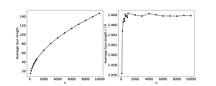
Figure 4: Numerical evaluation of the average-case performance of X-opt.

5 Discussion

Although the results we presented in Theorem 2.1 and Theorem 3.3 are rather negative for X-opt, the numerical experiments of Section 4 paint a much more optimistic picture. The heuristic appears to be much more efficient in practice than our lower bounds suggest. Indeed, while Theorem 3.3 suggests an approximation ratio of $\Omega(\sqrt{n})$, the numerical experiments in Section 4 suggest a constant approximation ratio.

One possible explanation for this discrepancy is that we compare the optimal solution on any instance to local optima specifically constructed to be bad. This is a rather standard approach, and it is not surprising that it gives pessimistic results. However, the results in this case are especially pessimistic, considering that we can show a tight lower bound for the expected tour length in the average case.

We consider this to be an indication that this approach is incapable of explaining the practical approximation performance of local search heuristics. In order to more closely model the true behavior of heuristics, it seems one must analyze the landscape of local optima, and the probability of reaching different local optima. We stress that this discrepancy cannot be resolved by other standard methods of probabilistic analysis. In particular, smoothed analysis [10] cannot help, since the smoothed approximation ratio of an algorithm is bounded from below by the average-case approximation ratio.

References

- [1] Aarts, E., Lenstra, J.K. (eds.): Local Search in Combinatorial Optimization. Princeton University Press (2003). https://doi.org/10.2307/j.ctv346t9c
- [2] Biniaz, A., Maheshwari, A., Smid, M.: Flip Distance to some Plane Configurations (May 2019). https://doi.org/10.48550/arXiv.1905.00791
- [3] Brodowsky, U.A., Hougardy, S., Zhong, X.: The Approximation Ratio of the k-Opt Heuristic for the Euclidean Traveling Salesman Problem (Aug 2021). https://doi.org/10.48550/arXiv.2109.00069
- [4] Chandra, B., Karloff, H., Tovey, C.: New Results on the Old k-opt Algorithm for the Traveling Salesman Problem. SIAM Journal on Computing 28(6), 1998–2029 (Jan 1999). https://doi.org/10.1137/S0097539793251244
- [5] da Fonseca, G.D., Gerard, Y., Rivier, B.: On the Longest Flip Sequence to Untangle Segments in the Plane (Dec 2022). https://doi.org/10.48550/arXiv.2210.12036
- [6] Englert, M., Röglin, H., Vöcking, B.: Smoothed Analysis of the 2-Opt Algorithm for the General TSP. ACM Transactions on Algorithms 13(1), 10:1–10:15 (Sep 2016). https://doi.org/10.1145/2972953
- [7] Frieze, A.M., Yukich, J.E.: Probabilistic Analysis of the TSP. In: Gutin, G., Punnen, A.P. (eds.) The Traveling Salesman Problem and Its Variations, pp. 257–307. Combinatorial Optimization, Springer US, Boston, MA (2007). https://doi.org/10.1007/0-306-48213-4_7
- [8] Korte, B., Vygen, J.: Combinatorial Optimization: Theory and Algorithms. Algorithms and Combinatorics, Springer-Verlag, Berlin Heidelberg (2000). https://doi.org/10.1007/978-3-662-21708-5
- [9] Papadimitriou, C.H.: The Euclidean travelling salesman problem is NP-complete. Theoretical Computer Science 4(3), 237–244 (Jun 1977). https://doi.org/10.1016/0304-3975(77)90012-3
- [10] Spielman, D.A., Teng, S.H.: Smoothed analysis of algorithms: Why the simplex algorithm usually takes polynomial time. Journal of the ACM 51(3), 385–463 (May 2004). https://doi.org/10.1145/990308.990310
- [11] Van Leeuwen, J., Schoone, A.: Untangling a traveling salesman tour in the plane. Proc. 7th Internat. Workshop Graph-Theoret. Concepts Comput. Sci. (Jan 1980)