X-ray time lag evaluation of MAXI J1820+070 with a differential cross-correlation analysis

Abstract

MAXI J1820$+$070 is a transient black hole binary (BHB) discovered on 2018 March 11. The unprecedented rich statistics brought by the NICER X-ray telescope allows detailed timing analysis up to $\sim$1 kHz uncompromised by the photon shot noise. To estimate the time lags, the Fourier analysis was applied, which led to two different conclusions for the system configuration; one supporting the lamp-post configuration with a stable accretion disk extending close to the innermost stable circular orbit and the other supporting the truncated accretion disk contracting with time. Using the same data set, we present the results based on the cross-correlation function (CCF). The CCF is calculated between two different X-ray bands and one side is subtracted from the other side, which we call the differential CCF (dCCF). The soft and hard lags respectively of $\sim$0.03 and 3 s are clearly identified without being diluted by the spectral mixture, demonstrating the effectiveness of the dCCF analysis. The evolution of these lags is tracked, along with spectral changes for the first 120 days since the discovery. Both the dCCF and spectral fitting results are interpreted that the soft lag is a reverberation lag between the Comptonized emission and the soft excess emission and that the hard lag is between the disk black body emission and the Comptonized emission. The evolution of these lags is in line with the picture of the truncated disk contracting with time.

1 Introduction

MAXI J1820+070 (hereafter J1820) is a transient black-hole binary (BHB) that exhibited outbursts four times in a row from March 2018 to October 2019. It was first reported in the optical band by ASSASSN (Tucker et al., 2018) and observed in the X-ray band by the Monitor of All-sky X-ray Image (MAXI) (Matsuoka et al., 2009) a few days later. Due to its extreme brightness (4 Crab at the maximum; Shidatsu et al. 2019) and low galactic absorption ($N_{H}\sim 10^{-21}~{}\text{cm}^{-2}$; Uttley et al. 2018) at a short distance ($3\pm 1$ kpc; Gandhi et al. 2019), J1820 was intensively observed with a suite of observatories and was found to exhibit many behaviors similar to other BHBs. The Neutron star Interior Composition Explorer (NICER; Gendreau et al. 2016) observed J1820 most frequently, providing a unique data set that enables detailed X-ray timing-spectroscopy analyses up to a $\sim$1 kHz range against the photon shot noise.

The combination of the favorable features of J1820 and the rich data set of NICER are ideal to investigate some of the unsolved problems of BHBs. One of them is the geometry of the hot corona in the low/hard state, which is considered to be the production site of the Comptonized emission that dominates the X-ray band. Two competing pictures are proposed; one is the hot accretion flow and truncated-disk model (Plant et al., 2014; Ingram & Done, 2011), in which the optically-thick disk is truncated at a radius far away from the innermost stable circular orbit (ISCO) from which matter falls along the advection-dominated accretion flow (ADAF). Thermal photons are thought to come from the optically-thick disk, which are Comptonized in the hot corona in the ADAF. The other is the lamp-post model with a different configuration (Fabian et al., 2014; García et al., 2015); the accretion disk is close to the ISCO radius and a small hot corona exists along the rotation axis of the black hole.

The above two models have been pursued for J1820. Kara et al. (2019) found that the reverberation time lag from the Comptonized emission to its disk reflected emission is shorter than that observed in other BHBs. Together with a stable Fe K$\alpha$ line profile produced by reprocessing the Comptonized emission off of the disk, they supported the lamppost configuration (Kara et al., 2019; Buisson et al., 2019). This interpretation was challenged by many others using the same data set with various techniques (De Marco et al., 2021; Axelsson & Veledina, 2021; Zdziarski et al., 2021; Kawamura et al., 2022a, b), all of which point to the truncated-disk model with the inner disk radius much larger than the ISCO.

Amongst many analysis techniques, the reverberation time lag is a key for providing a direct constraint on the geometry. It is conventionally analyzed by using the cross spectrum in the frequency domain. Curiously, the two camps used this technique with the same data set, but reached different conclusions. On one hand, Kara et al. (2019) reported a shorter reverberation lag of $\mathcal{O}$(1 ms) using the phase shift in the cross spectrum and argued for the lamppost geometry. On the other hand, De Marco et al. (2021) reported a longer lag of $\mathcal{O}$(10 ms) using the zero-crossing points in the cross spectrum and argued for the truncated-disk geometry.

The time lags derived from the cross-spectrum need some caution, regardless of whether the estimate is based on the phase shift or the zero crossing points, as we will describe in § 2. Here, we propose an approach based on the cross-correlation function (CCF) as an alternative method to determine the time lag. This is a time-domain technique complementary to the cross-spectrum and free from the cautions associated with the frequency-domain technique. The CCF has not been an often-used approach within X-ray bands since its early applications (e.g. Priedhorsky et al., 1979; Maccarone et al., 2000) mainly because the small contrast between the two spectral components with a time lag yields a small cross correlation that is overwhelmed by an autocorrelation of the component of interest. However, with the availability of the NICER data with rich photon statistics and a subtraction of the autocorrelation contributions, we revisit the utility of this technique in actual applications to J1820. In addition to the CCF-based time lag, we also perform spectral analysis to confirm that the CCF-based time lag result can be interpreted in a picture consistently with the spectral analysis result.

The plan of the paper is as follows. In § 2, we give a formalism of the CCF and compare it with the cross-spectrum. In § 3, we describe the NICER data, to which we apply the CCF. In § 4, we start with an overview of the data set (§ 4.1). We first apply the CCF and spectral analysis at one epoch (§ 4.2) and expand the function to the entire range of interest (§ 4.3) to track the development of the CCF parameters. In § 5, we discuss interpretation of the result. We show that both the CCF-based time lag and the spectral results can be interpreted with the truncated-disk model with contracting inner radius as the low/hard state proceeds up till the transition to the soft state. The summary and conclusion are given in § 6.

2 Method

We briefly compare two approaches for the time lag analysis; one is the conventionally-used cross spectra in the frequency domain and the other is the CCF in the time domain used in this paper. Readers are referred to Poutanen (2002) for derivation of the equations for a typical disk geometry. We give a brief derivation below for the sake of completeness.

We take two X-ray light curves in the different energy bands 1 and 2. We assume that the band 1 is dominated by the direct emission $x(t)$, whereas the band 2 is a linear composition of the direct emission and its reprocessed emission lagged from the direct emission by a fixed time $t_{\mathrm{lag}}$. The light curve of each band is given by

$$\begin{array}[]{ccl}y_{1}(t)&=&x(t)\\ y_{2}(t)&=&\alpha x(t)+\beta x(t-t_{\mathrm{lag}}),\end{array}$$ (1)

where $\alpha$ and $\beta$ are linear coefficients.

The cross spectrum, on one hand, is calculated in the frequency domain as

$$\begin{split}S_{1,2}(f)&=Y_{1}^{*}(f)Y_{2}(f)\\ &=\overline{x(t)^{2}}\left[\alpha+\beta e^{-i2\pi ft_{\mathrm{lag}}}\right],\\ \end{split}$$ (2)

in which $Y_{i}(f)$ denotes the Fourier transform of $y_{i}(t)$ for $i=1,2$, and ${\overline{x(t)^{2}}}$ is the time average for $x(t)^{2}$. The argument of $S_{1,2}$ is translated as the lag amplitude by

$$\Delta t(f)=\frac{1}{2\pi f}\arctan\left({\frac{\beta\sin{(2\pi ft_{\mathrm{lag}})}}{\alpha+\beta\cos{(2\pi ft_{\mathrm{lag}})}}}\right).$$ (3)

Only when $\alpha=0$, i.e., the band 2 is composed only of the reprocessed emission, $\Delta t$ matches $t_{\mathrm{lag}}$. At the zero frequency limit,

$$\Delta t(f)\rightarrow\frac{\beta}{\alpha+\beta}t_{\mathrm{lag}}~{}~{}(f\rightarrow 0).$$ (4)

In many cases, the reprocessed emission is subtle compared to the direct emission within the X-ray band ($\alpha\gg\beta$), thus the $t_{\mathrm{lag}}$ is diluted in $\Delta t(f)$ by a large factor ($\frac{\beta}{\alpha+\beta}$) (Miller et al., 2010). Therefore, the face value of the lag amplitude in the cross spectrum should not be used to derive the reverberation distance. The first zero-crossing point of $\Delta t(f)=0$ at $f=\frac{1}{2t_{\mathrm{lag}}}$ is a more robust estimate of the lag amplitude (Mizumoto et al., 2018). In practice, though, it is not easy to track the oscillatory behavior of $\Delta t(f)$ to identify the first zero-crossing point in a small dynamic range of $f$ limited by the observation duration and the time binning against the photon shot noise.

The CCF, on the other hand, is defined as the inverse Fourier transform of $S_{1,2}(f)$ in the time domain. The real part is expressed as

$$\begin{split}C(\tau)&=\Re\left\{\int_{-\infty}^{\infty}S_{1,2}(f)e^{i2\pi f\tau}dt\right\}\\ &=\alpha A(\tau)+\beta A(\tau-t_{\mathrm{lag}}),\\ \end{split}$$ (5)

where $A(\tau)$ is the auto-correlation function (ACF). Two peaks at $\tau=0$ and $t_{\mathrm{lag}}$ appear separately with an amplitude contrast of $\alpha/\beta$.

The cross spectra have been more dominantly used to date in assessing the reverberation time lags in the X-ray band (Uttley et al., 2014). This is because the contrast $\beta/\alpha$ is usually too small within the X-ray bands. Only when high contrast is expected between two different wavelengths, the CCF becomes a powerful technique. This was indeed the case in J1820 between X-ray and UV or optical bands (Kajava et al., 2019; Paice et al., 2021). Now, when combined with rich photon statistics that NICER brings for the first time, the CCF, or a variant thereof, can be used between two different X-ray bands even for a small contrast. We will demonstrate this by using the NICER data of J1820.

3 Observations and data reduction

We use the data obtained with NICER, with which J1820 was observed many times. The entire view of the NICER data set can be found in Stiele & Kong (2020). We use the period from MJD 58190 to 58304, which covers the first brightening followed by the gradual decline and the onset of the second brightening. This period has been intensively studied by several authors, leading to the dispute of its interpretation described in § 1.

NICER is an X-ray timing-spectroscopy mission operated in the international space station since 2017. It consists of 56 independent X-ray Timing Instruments (XTI), each of which has the X-ray concentrator optics and the silicon drift detector (Gendreau et al., 2016). In addition to its specific mission goals (Gendreau et al., 2016), NICER is useful in a wide range of astrophysics. Its large effective area and large dynamic range allow timing analysis beyond 1 kHz, which has been inaccessible with other X-ray instruments due to photon shot noise or slow response. Moreover, its moderate energy resolution (140 eV at 6 keV) and bandpass (0.5–12 keV) make broad-band spectral analyses possible. For the purpose of this study, NICER is uniquely suited.

We retrieved the pipeline products from the archive for the observation sequences 1200120101–1200120196. Detailed information on the data set can be found in De Marco et al. (2021). We used HEASoft version 6.29 for data analysis. We generated the redistribution matrix function (RMF) and the auxiliary response function (ARF) for each data set. We used the background file provided by the instrument team.

4 Analysis

We start with a brief overview of the data set (§ 4.1). We first use the data at one epoch to describe the analysis in detail (§ 4.2), which will be expanded in the entire duration (§ 4.3).

4.1 Overview of data

After the first X-ray detection of J1820 (Kawamuro et al., 2018) on March 11, 2018, the X-ray flux increased rapidly for two weeks to reach the peak flux of $\sim$4 Crab on March 26. The spectral hardness remained hard and the flux gradually decreased for the next $\sim$90 days (the low hard state in Shidatsu et al. 2019) when the source made a drastic transition to the high soft state. The source exhibited further changes later, which is out of the scope of this paper. We focus on the entirety of the low hard state and the onset of the transition to the high soft state, in which a dense coverage by NICER was made for $\sim$120 days. The detailed description of the data set is given extensively in the literature (Kara et al., 2019; Stiele & Kong, 2020; Axelsson & Veledina, 2021; De Marco et al., 2021). Here, we only give two characterizations —the light curve and the color-color diagram— for the sake of completeness of this paper.

Figure 1 shows the X-ray light curve in the soft (0.5–1.0 keV) and hard (1.0–10.0 keV) bands ($S(t)$ and $H(t)$, respectively) and the spectral hardness defined as $\left\{H(t)-S(t)\right\}/\left\{H(t)+S(t)\right\}$. After the rapid brightening at the beginning, the flux change was slow with a noticeable break between MJD 58240 and 58260. In the last part after MJD 58280, the source started a transition to a new state, which is dubbed as the intermediate state (Shidatsu et al., 2019). Hereafter, we follow the phase definition by De Marco et al. (2021): i.e., rise (until MJD 58201), plateau (until MJD 58251), bright decline (until MJD 58289), and hard-soft transition (until MJD 58305).

Figure 2 shows evolution of the spectral change. Three bands are defined as soft (0.5–2 keV), medium (2.0–3.5 keV), and hard (3.5–10 keV) and the ratios of the adjacent two bands are plotted. The color codes are given to aid chronological interpretation. The initial rapid change (red), the gradual and monotonic decay with a break between MJD 58240 and 58260 (yellow), and the start of the state transition (green) are clearly traced.

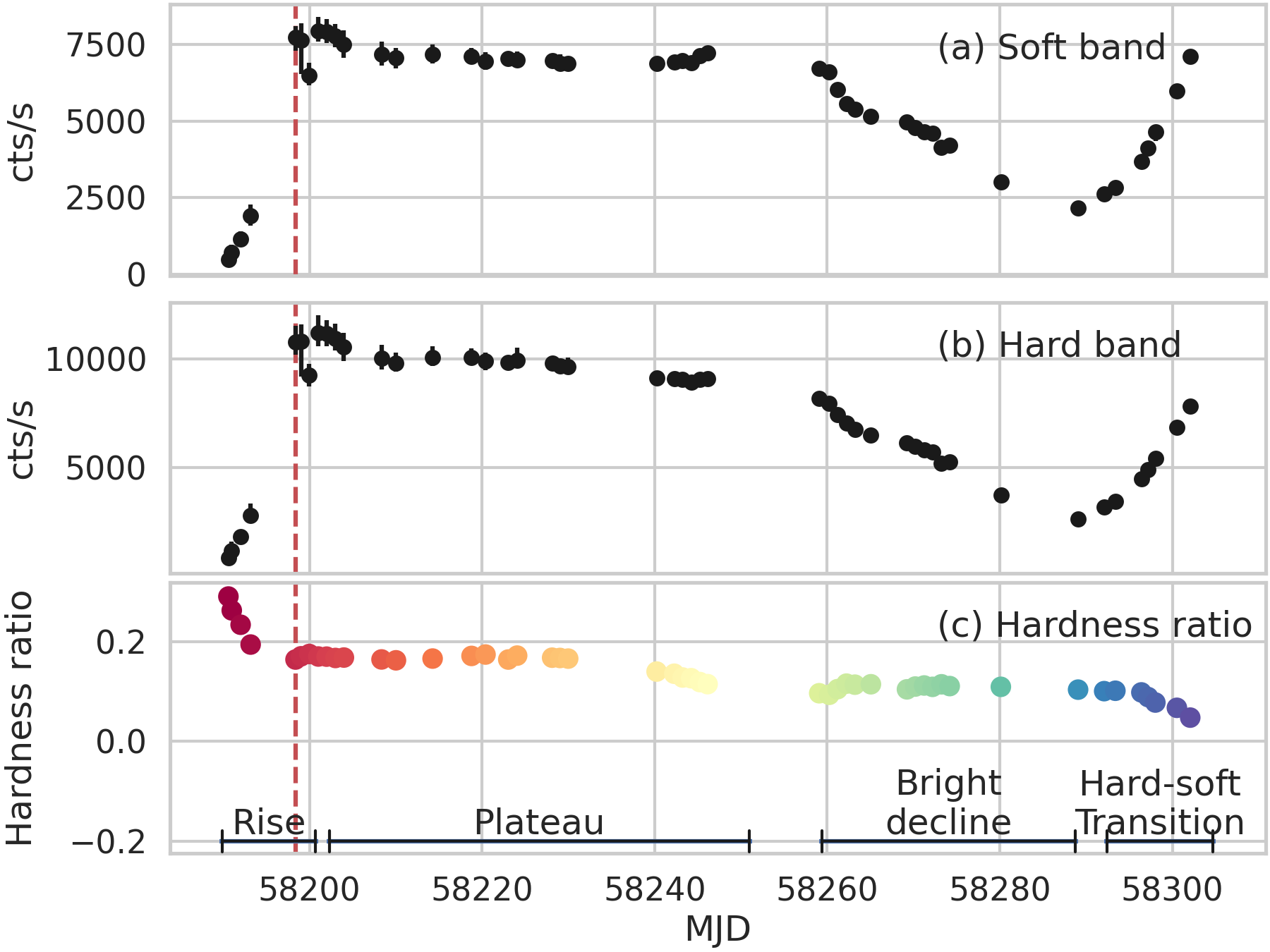
Figure 1: X-ray light curves in the soft (0.5–1 keV) and hard (1–10 keV) bands (top and middle panels, respectively) and the hardness ratio (bottom panel). Each point is calculated for a mean value among 64 s bins of the light curve in a certain duration. Colors in the hardness ratio represent MJD in the same manner as in Figure 2. The phase definitions are given in the bottom panel. The red vertical dashed line shows MJD 58197 (2018 March 21) used in the detailed analysis (§ 4.2).

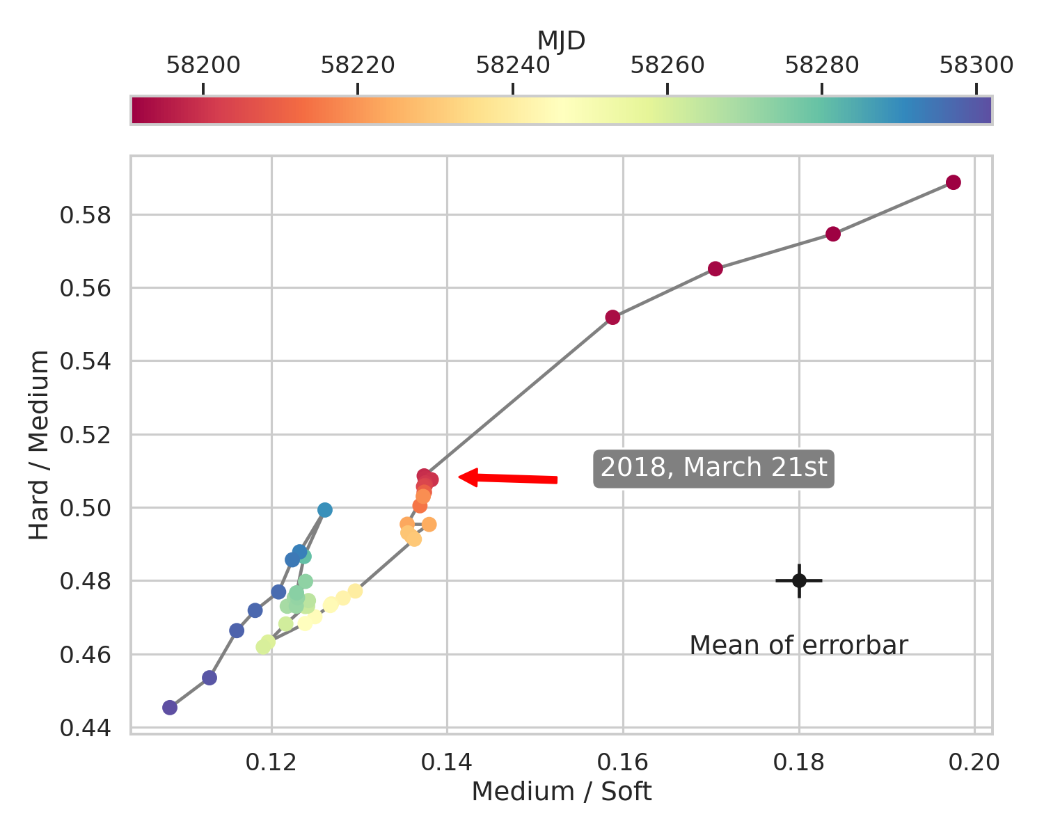
Figure 2: X-ray color-color diagram. Here, we defined the soft, medium, and hard bands as 0.5–2, 2.0–3.5, and 3.5-10.0 keV, respectively. Two colors are calculated as the ratio of the two adjacent bands. The black curve gives the track connecting data points. MJD 58197 (2018 March 21) is shown by the red arrow, which is used for the detailed analysis (§ 4.2).

4.2 Observation of 2018 March 21

We use the data (OBSID 1200120106) at the peak flux on 2018 March 21 (MJD 58197) to establish the data analysis method. We first fit the X-ray spectrum with a phenomenological model to decompose it into major spectral components and select energy bands where they are most dominant (§ 4.2.1). We then apply CCF analysis between these bands (§ 4.2.2).

4.2.1 Spectral decomposition

A phenomenological model fitting was performed in 0.7–10 keV to define appropriate energy bands for the CCF analysis. In the hard state, the Comptonized component in the power-law form is dominant in the entire energy range (Axelsson & Veledina, 2021). Deviations are seen in the soft band with another broad component attributable to the disk emission, and in the Fe K band with both narrow and broad emission lines (Axelsson & Veledina, 2021). In addition, an excess emission in the softest band is required for complete spectral modeling (De Marco et al., 2021).

We include all these components to fit the spectrum. The multi-color disk black body component was represented using the diskbb model in the XSpec spectral fitting package. A part of the disk emission is inverse Compton scattered into power-law emission, which was modeled with the simpl model. The soft excess component was represented by a broad Gaussian component. The narrow and broad lines at the Fe K band are the Gaussian components with their center fixed at 6.4 keV. The summation is attenuated by an interstellar extinction by TBabs (Wilms et al., 2000) with the hydrogen-equivalent column fixed at $1.5\times 10^{21}$ cm^-2 (Uttley et al., 2018).

The three broad components (disk black body, Comptonized, and soft excess) are coupled with each other at the softest band in the spectral fitting. In order to decouple them as much as possible, we first fitted the spectrum in the 2.2–10.0 keV band where the soft excess emission is negligible, and constrained the disk black body and its Comptonized components along with the Fe K emission lines. We then extrapolated the best-fit model to the entire 0.7–10.0 keV band and added the soft excess component. The spectrum, the best-fit model, and the residuals to the fit are shown in Figure 3. The detector response calibration and the fitting models are presumably imperfect at this moment, leaving some structures below $\sim$3 keV in the residual, which we ignore in this paper, because the purpose here is to define the appropriate energy bands for the following CCF analysis.

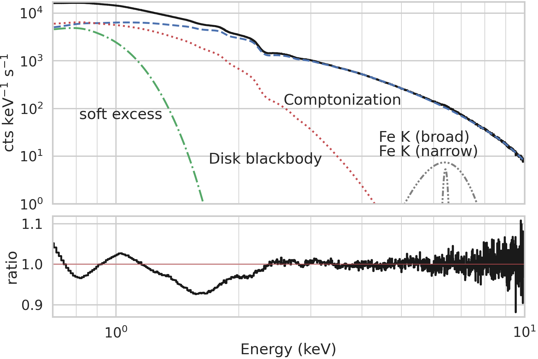
Figure 3: Observed spectrum on MJD58197 and the best-fit model (top), and residuals of the fit (bottom). Models of each spectral component are shown with different symbols.

The Comptonized component dominates the entire energy range. The disk emission is sub-dominant below $\sim$5 keV and the soft excess emission below $\sim$2 keV. We thus define five fine energy bands: 0.5–1, 1–2, 2–3, 3–5, and 5–10 keV having different mixtures of these spectral components. Alternatively, we also use the two coarse bands, the soft band (0.5–1 keV) and the hard band (1–10 keV).

4.2.2 CCF

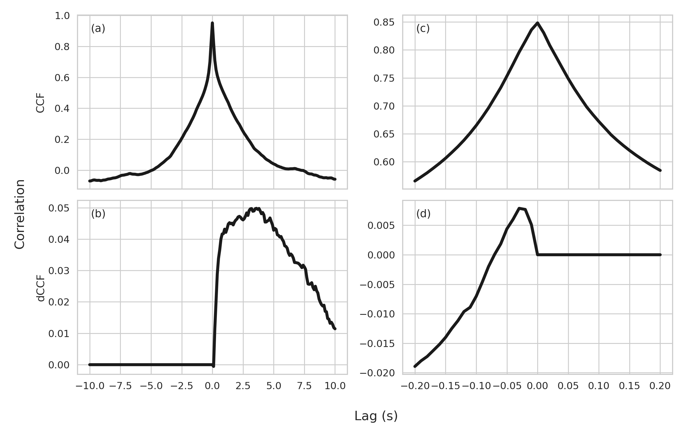
Figure 4: (top) CCF and (bottom) dCCF between the two coarse energy bands —soft (0.5–1.0 keV) and hard (1.0–10.0 keV) bands— in the longer ($\tau<10$ s; left) and the shorter ($\tau<0.2$ s; right) time scales.

We calculated the CCF between the two coarse bands (soft and hard), and show the result in two different time scales: (1) $-10\leq\tau\leq+10$ s (panel a) and (2) $-0.2\leq\tau\leq+0.2$ s (panel c) in Figure 4. Because both bands are dominated by the same spectral component (Comptonized component), the CCF is dominated by its auto correlation peaking at 0 s. However, there are noticeable asymmetry in both time scales, which are clarified by subtracting the left half ($\tau<0$ s) from the right half ($\tau>0$ s) or vice versa as shown in panels (b) and (d). The subtraction sign was swapped arbitrarily to make the lag to be positive; i.e., we interpret the negative soft lag as positive hard lag. We call them differential CCF (dCCF).

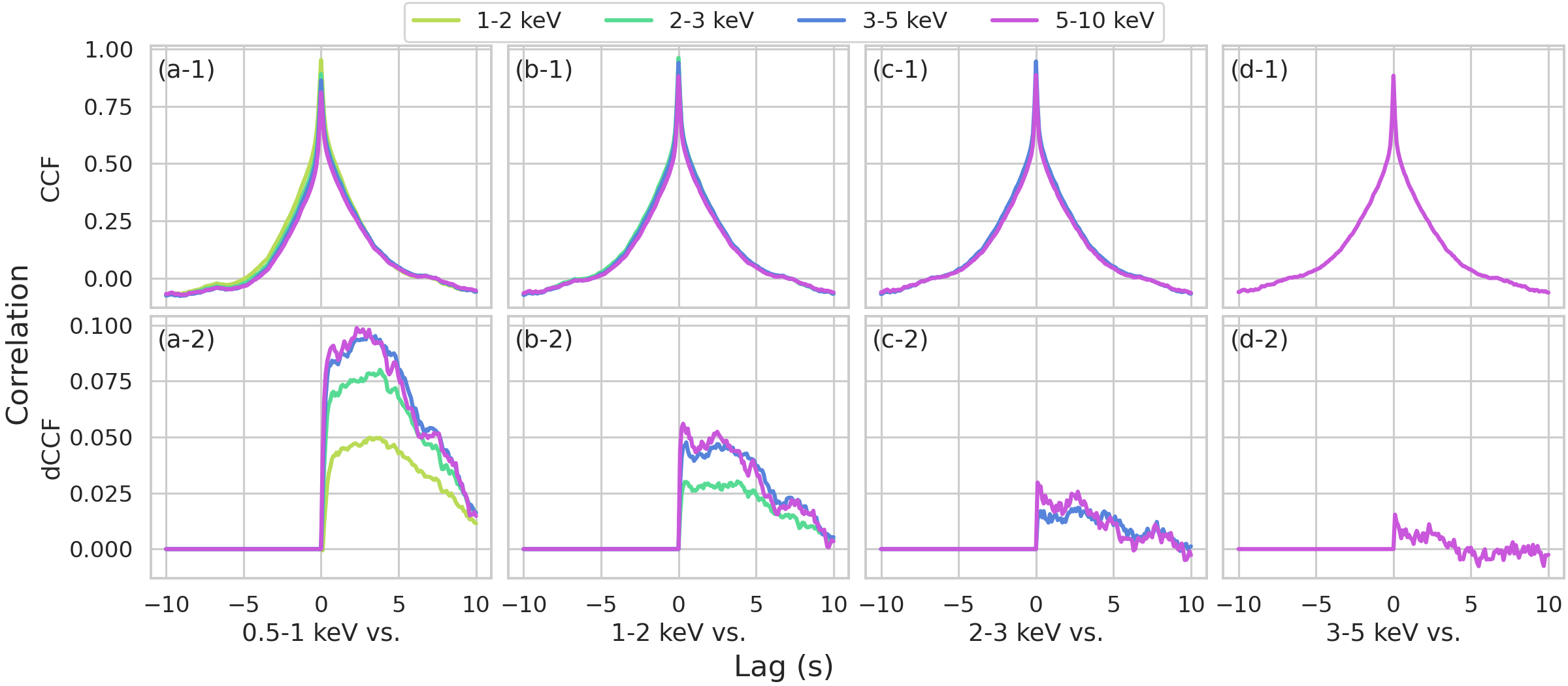
Figure 5: CCF (top) and dCCF (bottom) between two of the five fine energy bands in the longer time scale of $|\tau|\leq 10$ s with a time bin of 0.1 s. The reference band is given at the bottom of each column, while the target band is shown with different colors.

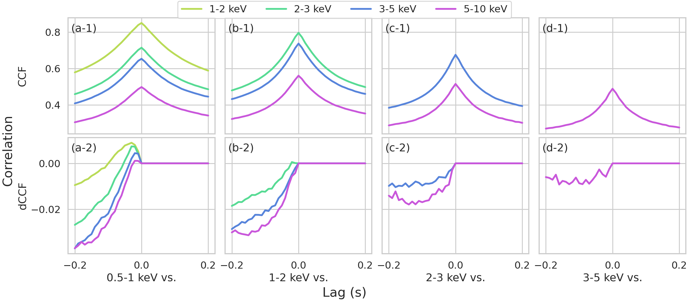
Figure 6: Same as Figure 5 for the shorter time scale of $|\tau|\leq 0.2$ s with a time bin of 0.01 s.

Two distinct structures are found in the dCCF. One is a positive hard lag in the longer time scale (panel b) and the other is a positive soft lag in the shorter time scale (panel d). These lag phenomena correspond to the hard and soft lags found using the cross spectra (Kara et al., 2019; De Marco et al., 2021), where their amplitudes were 3 s and 30 ms, respectively. We emphasize that the same amount of the lags free from the spectral dilution are easily recognized in the dCCF. Furthermore, the two lag amplitudes are not a single value (not a delta function) but have some structures in the dCCF, which may carry information on the lag response.

Next, we use the finer energy bands to investigate energy dependence of these lags. Two energy bands out of the five were selected as the reference and the target band for the CCF. Figures 5 and 6 respectively show the hard lag in the longer time scale and the soft lag in the shorter time scale, where the CCF (top panels) and the dCCF (bottom panels) between different bands are calculated. Note that the dCCF for the soft lag is affected by the one for the stronger hard lag with a longer time scale. Still, we see positive soft lag clearly in the dCCF at panel (a-2) in Figure 6.

4.3 Development of the spectral and temporal behaviors

Figure 7: Development of (a) the count rate in the 0.5-10.0 keV band, (b–c) the spectral parameters ($R_{\mathrm{in}}$ and $T_{\mathrm{in}}$ in the diskbb*simpl model fitting, and (d–f) the CCF and dCCF parameters; the zero-lag correlation in CCF (d), the mean hard and soft lags in (e and f, respectively). The CCF and dCCF for only 0.5-1.0 keV and 1.0-2.0 keV are shown. We plot the error bars in the (b) and (c), which are hardly seen due to the small values. The red vertical dashed line shows MJD 58197 (2018 March 21) used in the detailed analysis § 4.1. Pairs of the same energy band in all figures use the same color shown in the legend.

We apply the spectral and temporal analyses developed in one epoch (§ 4.2) to the entire data set. The same analysis worked for the most part of the changing behavior J1820 in the duration of interest. Figure 7 shows the development of the count rate in panel (a) along with the results of the spectral analysis in the panels (b–c) and those of the temporal analysis in the panels (d–f). The phase definition describing the count rate development is given in (a).

For the spectral analysis, best-fit values of some key parameters are shown: (a) the count rate of the entire energy band, (b) the inner disk radius $R_{\mathrm{in}}$ and (c) the temperature $T_{\mathrm{in}}$ from the diskbb model. Here, we derived $R_{\mathrm{in}}$ from $(R_{\mathrm{in}}/D_{10})^{2}\cos{(\theta)}$, where $D_{10}=0.3$ is the distance in the 10 kpc unit (Gandhi et al., 2019; Atri et al., 2020) and $\theta=70$ deg is the inclination angle (Torres et al., 2019). No model fitting is performed in the rise phase due to rapid spectral changes within the duration for the fitting.

For the temporal analysis, (d) the correlation at the zero lag in the CCF ($r_{0}$), (e) the absolute value of the hard lag at the dCCF peak ($|\tau_{\mathrm{hard}}|$), and (f) the one for soft ($|\tau_{\mathrm{soft}}|$) are plotted. The $|\tau_{\mathrm{soft}}|$ values are quantized at 10 ms due to the statistical limit. Since all the energy band pairs exhibit similar behavior, we only plot the development of the dCCF between 0.5–1.0 keV and 1.0–2.0 keV.

The overall development of the spectral parameters follows that of the count rate. Through the plateau and bright decline phases, the count rate change appears mostly governed by the decreasing $R_{\mathrm{in}}$. In the hard-soft transition phase, it is difficult to distinguish which of the $T_{\mathrm{in}}$ and $R_{\mathrm{in}}$ are more responsible for the count rate changes; these two parameters are coupled in the spectral fitting, which makes the interpretation complicated. For the temporal parameters of the CCF and dCCF, the development of both the soft and the hard lags (panels e and f) exhibits a decline in the plateau phase. Beyond the bright decline phase, though, both lag estimates do not show systematic variations.

5 Discussion

5.1 Relation between spectral and time-lag components

In § 4.2, we dissected the same data set taken at a particular epoch either in spectral (§ 4.2.1) and temporal (§ 4.2.2) domain. For the CCF and dCCF, we investigated the energy dependence (Figures 5 and 6).

An interesting contrast is observed in the two lags. In the hard lag, the largest correlation is seen between the 0.5–1.0 and 5–10 keV pairs, where the correlation increases as the target band is away from the reference band (Figure 5 a-2). This suggests that the hard lag is produced between two spectral components below and above $\sim$3 keV, and that the harder spectral component becomes more dominant at higher energies. In the soft lag, in contrast, the largest correlation is seen between the 0.5–1.0 and 1.0–2.0 keV bands, where the correlation decreases as the target band is away from the reference band (Figure 5 a-2). This suggests that the soft lag is produced between two components, one of which is localized below 1 keV and the other extending from below 1 keV up to above 5 keV.

In combination with the spectral result, we interpret that the hard lag is between the disk black body component and the Comptonized component, while the soft lag is between the Comptonized component and the soft excess component. We verify our interpretation with simulation. The goal is to examine if the observed features in the dCCF (Figures 5 and 6) can be reproduced from synthesized light curves of each energy band with the mixing ratio of the three spectral components fixed to the ratio derived from the spectral fitting (§ 4.2.1).

To generate the synthesized light curves, we constructed the power spectral density (PSD) of J1820 using the observation. Figure 8 shows the PSD for the observed light curve in the 5.0–10.0 keV, in which the emission is almost purely made of the Comptonized component (Figure 3). As is often seen in BHBs, the PSD is represented by a broken power law, in which the power of the PSD as a function of the frequency breaks at a cut-off frequency. In Figure 8, the cut-off is around $0.02$ Hz.

The Ornstein-Ulenbeck (OU) process is suitable for generating synthesized light curves having a PSD of a broken power law shape and was applied to model light curves of BHBs (Kelly et al., 2011). The autocovariance function is expressed as

$$R_{\rm OU}(t)=Ae^{-|t|/t_{\text{scale}}},$$ (6)

where $A$ is the amplitude of the variance and $t_{\text{scale}}$ is the timescale of the variation, or the inverse of the cut-off frequency. Computing the Fourier transform of the auto-covariance, we derive the PSD of the OU process as

$$\begin{split}P_{\rm OU}(\omega)&=\frac{1}{2\pi}\int^{\infty}_{-\infty}e^{-i\omega t}R_{\rm OU}(t)dt\\ &=B\frac{1}{\omega^{2}+\omega_{0}^{2}},\end{split}$$ (7)

where $B=A/2\pi\,t_{\text{scale}}$ and $\omega_{0}=1/t_{\text{scale}}$. The PSD decays as $1/\omega^{2}$ for $\omega\gg\omega_{0}$.

Figure 8: PSDs in the 5.0–10.0 keV, where the Comptonized component is dominant, for the observation (purple) and the range of the simulation (gray) with the 80 % confidence intervals derived from 100 realizations. A second component is necessary in the simulation to account for the observed PSD at the high frequency end, but was omitted as the slight deviation does not affect the result.

Figure 9 (top) shows the generated light curves for the three spectral components with $t_{\mathrm{scale}}=$5 s (=$1/0.02$ Hz), a time bin of 0.01 s, and a duration of 163.84 s (=$2^{14}$ bins). Here, among the three spectral components, the Comptonized component is delayed from the disk component by 3 s and the soft excess component is delayed from the Comptonized component by 0.03 s. The observed delays have some spread as can be found in the dCCF (Figures 5 and 6), but we represented them with a delta function for simplicity. We linearly added them with the ratio derived from the spectral fitting (§ 4.2.1) to generate the light curves in the five fine energy bands. Then, the CCF and dCCF were calculated in the same way as in § 4.2.2 and presented in the same way as in Figures 5 and 6.

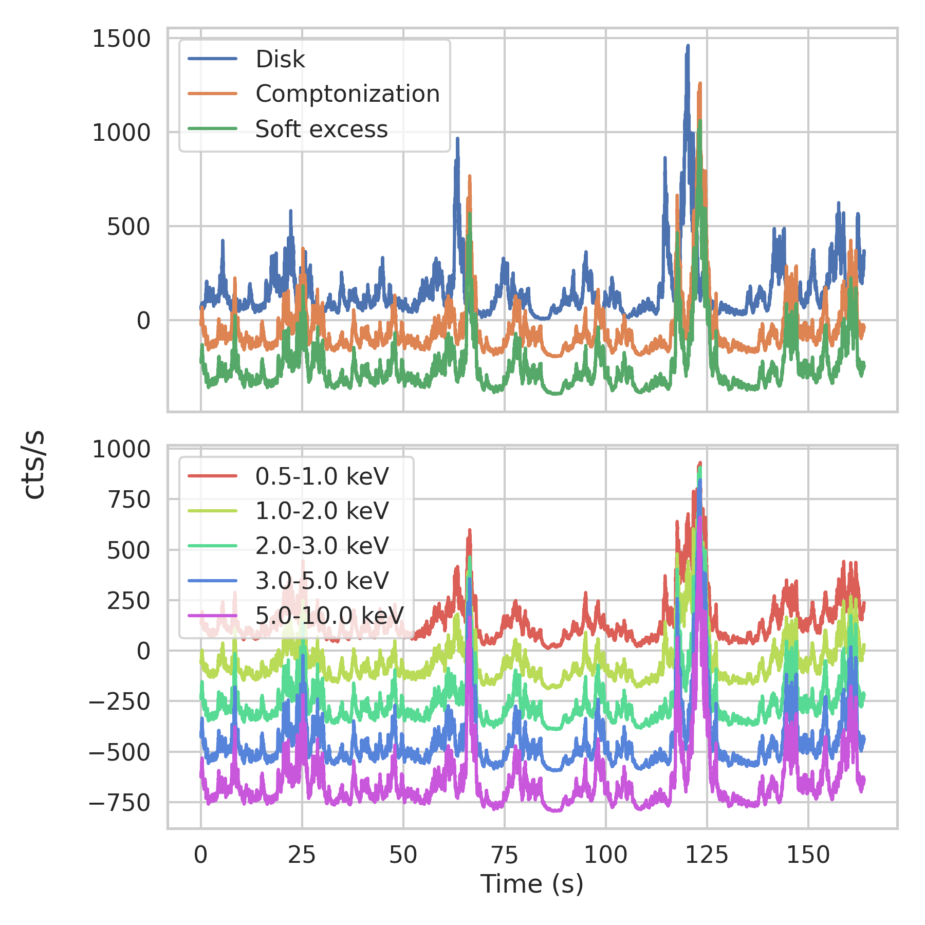
Figure 9: Top: The synthesized light curves

of the three spectral components, where offsets of –200 and –400 counts/s are added to the Compton scattering and soft-excess light curves for visibility. Bottom: The blended light curves in each energy band for one out of the 100 samples. Offsets of 0, –200, –400, –600, and –800 counts/s are added for 0.5-1.0 keV, 1.0-2.0 keV, 2.0-3.0 keV, 3.0-5.0 keV, and 5.0-10.0 keV light curves to highlight differences in variability.

Figures 10 and 11 show the result of the simulation, where their energy dependence is very similar to the observed one. In the hard lag, the correlation increases with the harder target band against the reference band. In the soft lag, a positive lag was found between the 0.5–1.0 keV and 1.0–2.0 keV bands. All these features are consistent with properties derived from the observed data, which reinforces our interpretation relating the spectral and temporal features.

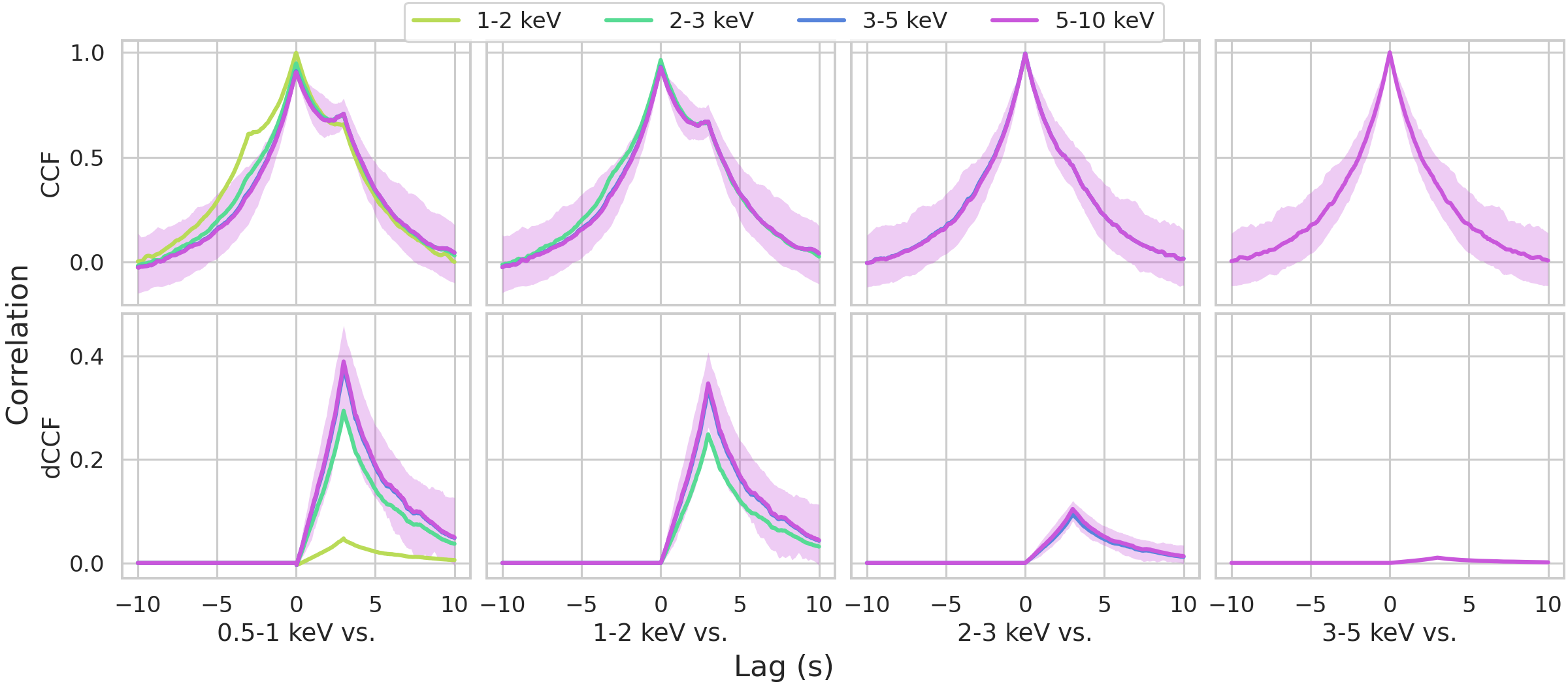
Figure 10: Same as Figure 5 but for the simulated light curves in Figure 9. The 80 % confidential ranges are shown only for the target band 5-10 keV.

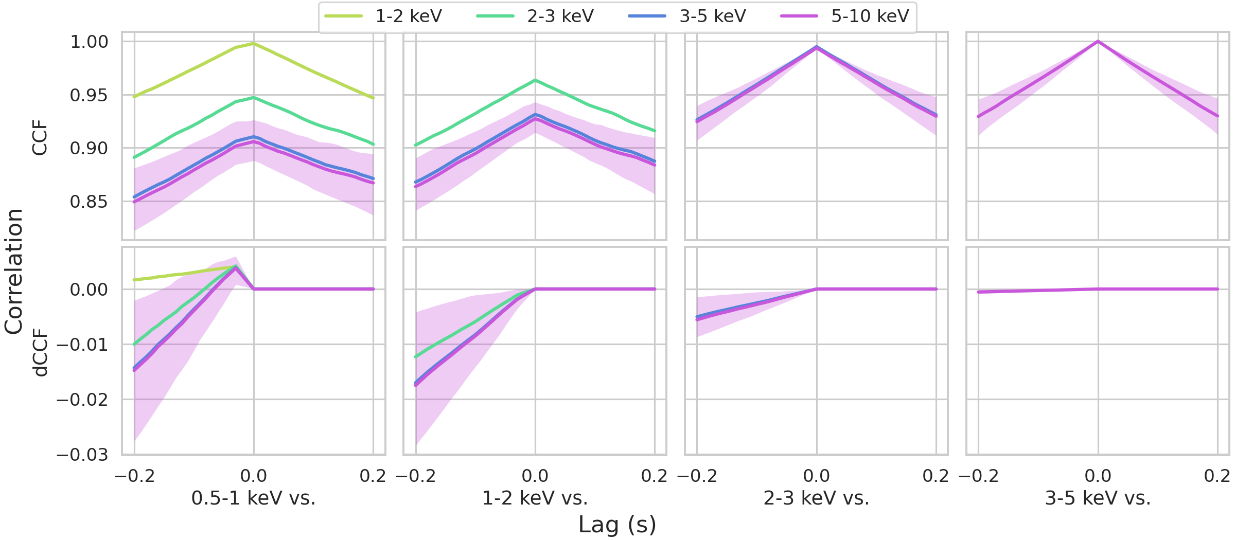
Figure 11: Same as Figure 6 but for the simulated light curves in Figure 9.

We should note that the Comptonized component alone can exhibit an energy-dependent in its ACF (e.g. Poutanen & Fabian, 1999; Kotov et al., 2001; Arévalo & Uttley, 2006; Mahmoud & Done, 2018; Veledina, 2018), thus yields a residual in the dCCF as calculated in § 4.2.2. However, if this is what we observe, the CCF asymmetry should be the strongest in the 3–5 versus 5–10 keV CCF, at which the Comptonized components are most dominant. Figure 5 (d–2) shows the contrary. One could further argue for multiple Comptonization components making the observed dCCF features due to energy-dependent lags between them, but there is no need to add a second Comptonization component in the spectral analysis presented in § 4.2.1, thus we do not favor such interpretation.

5.2 Interpretation for the parameter evolution

Based on the relation between the spectral and temporal properties (§ 5.1), we now interpret the results along with their evolution (Figure 7) for the soft (§ 5.2.1) and hard (§ 5.2.2) lags.

5.2.1 Soft lag

The soft lag was interpreted as the reverberation lag, in which the Comptonized photons in the corona irradiate the accretion disk to produce thermal soft excess emission. Both Kara et al. (2019) and De Marco et al. (2021) assessed the soft-lag amplitude by focusing on the different aspects of the cross spectrum. Kara et al. (2019) stated that the lag amplitude is short based on the phase shifts in the cross spectrum, which is subject to the underestimate due to the spectral dilution. De Marco et al. (2021) alleviated this effect by using the zero-crossing point in the cross spectra, but it was difficult to eliminate the effects of the overlapping hard lag signals.

It is thus important to check these results with the complimentary CCF. The dCCF technique has the advantage of being free from the spectral dilution and separating the two different time lags. Its estimated soft lag amplitude is $\sim$30 ms on 2018 March 21 (§ 4.2.2), which is closer to the value by De Marco et al. (2021). The value corresponds to the light-crossing scale of $\sim$300 times the Schwarzschild radius ($R_{\mathrm{s}}$) for a 10 $M_{\odot}$ black hole, which is more than an order larger than the value to support the lamp post configuration (Kara et al., 2019). If we use the soft lag amplitude derived by the dCCF technique, the reverberation distance changes from 300 to 100 $R_{\mathrm{s}}$ through the plateau phase (Figure 7 panel f). Both the spectral and temporal assessments have systematic uncertainty in the absolute valuesof $R_{\mathrm{in}}$, but their fractional changes match well(Figure 7 panel b). These are in line with the picture that the inner radius of the truncated accretion disk kept contracting through the phase.

5.2.2 Hard lag

The hard lag is a common feature in Galactic BHBs (Uttley et al., 2014) and was indeed found in J1820 too. The lag amplitude is too large for reverberation distances and is interpreted as a kind of propagation delay through the accretion disk flow (Kotov et al., 2001; Arévalo & Uttley, 2006). Kawamura et al. (2022a) successfully explained the observed hard lag, along with the X-ray spectrum and the PSD, by introducing a radial structure in the accretion corona flow from the inner radius of the accretion disk to the black hole. We interpret that the hard lag is produced between the disk emission and the Comptonized emission in the corona (§ 5.1). The steady decrease of the hard lag amplitude ($|\tau_{\mathrm{hard}}|$) in the plateau phase (Figure 7 panel e) is consistent with the contracting system,

We point out that the dCCF representation of the hard lag shows an association with the quasi-periodic oscillation (QPO). Stiele & Kong (2020) presented the evolution of the QPO fundamental frequency ($\nu_{\mathrm{QPO}}$) from 0.03 to 10 Hz in the duration of interest in this paper in their Figure 8. This QPO signal is also seen in the time domain in the dCCF. Figure 12 shows time series of the dCCF at different epochs represented sideways. Close to the 0 s in the lag, the main peak is recognized in every dCCF, which is the one shown in panel (e) in Figure 7. In addition, the secondary (and even higher orders in some) peaks are found. We have found that the time separation between the main peak and the secondary peak matches well with the QPO period ($1/\nu_{\mathrm{QPO}}$). This strongly suggests that the hard lag and the QPO are closely related, and both originate in the propagation in the accretion flow.

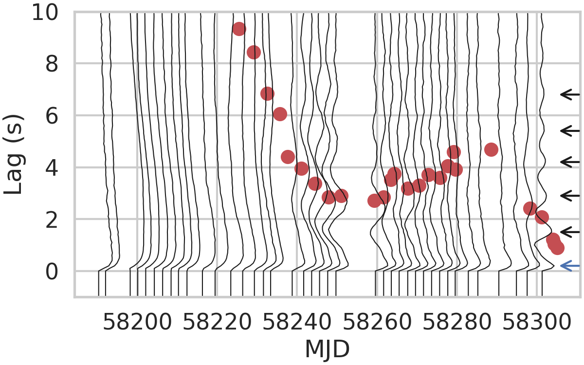
Figure 12: Development of the dCCF shown in the sideways in black curves, where often there are several peaks in the lags. For example, in the right-most dCCF, the primary (blue arrow) and higher-order (black arrow) peaks are marked. The primary is equivalent to $|\tau_{\mathrm{hard}}|$ in the panel (e) in Figure 7. The QPO periods in Stiele & Kong (2020) added to the primary peaks ($|\tau_{\mathrm{hard}}|+1/\nu_{\mathrm{QPO}}$) are shown in red circles. These match well with the secondary peaks.

6 Summary and Conclusion

We explored the NICER X-ray data of MAXI J1820$+$070, a transient BHB, to analyze time lags between two different X-ray bands during the first 120 days of discovery when the dense NICER coverage was made. We employed a time-domain approach (CCF) as opposed to the often used frequency domain approach (cross spectrum). We constructed the CCF between the soft (0.5–1.0 keV) and hard (1.0–10 keV) energy bands and removed the dominating autocorrelation component by subtracting the negative part of the CCF from the positive part, or vice versa, to derive the differential CCF (dCCF). In the dCCF, we clearly identified both the soft and hard lags respectively of $\sim$0.03 and $\sim$3 s separately without being diluted by the spectral mixture. The values are closer to the ones derived from the cross spectra analysis in De Marco et al. (2021) than those in Kara et al. (2019). This demonstrates the effectiveness of the dCCF complementary to the cross-spectrum in the X-ray time lag analysis, particularly when combined with the rich statistics that NICER brings.

We conducted the spectral and timing (dCCF) analyses separately at one of the brightest epochs in the duration of interest. In the spectral analysis, the X-ray spectra are represented by three components; the Comptonized power-law emission, the disk black body emission, and the soft excess emission (§ 4.2.1). In the timing analysis, we derived both the soft and the hard lags in the dCCF and constrained the energy dependence of the correlation by using a finer energy band resolution (§ 4.2.2). We then applied the analysis to the entire duration of interest to track the development of both the spectral and timing properties (§ 4.3).

Based on the spectral and timing analysis results, we conjectured that the soft lag is between the Comptonized and the soft excess emission, while the hard lag is between the disk and Comptonized emission. We verified this hypothesis by constructing the dCCF based on synthesized light curves of different energy bands made as a linear composition of the three spectral components lagged from each other. The energy dependence of the dCCF was recovered, which supports our hypothesis (§ 5.1).

Finally, we investigated the evolution of the spectral and timing properties along with time. Both the soft and the hard lags kept decreasing through the plateau phase. In the following bright decline phase, we could not follow the lag evolution due to the limited statistics. The evolution of the hard and soft lag amplitude is in agreement with the one of $R_{\mathrm{in}}$. All these features are consistent with a picture that the accretion disk is truncated and its inner radius kept contracting through the plateau phase (§ 5.2.1). Finally, we report a clear link between the hard lag and the QPO in the time domain (§ 5.2.2).

References

- Abadi et al. (2016) Abadi, M., Agarwal, A., Barham, P., et al. 2016, TensorFlow: Large-Scale Machine Learning on Heterogeneous Distributed Systems, arXiv, doi: 10.48550/arXiv.1603.04467
- Arnaud (1996) Arnaud, K. 1996, in Astronomical Data Analysis Software and Systems V, Vol. 101, 17
- Arévalo & Uttley (2006) Arévalo, P., & Uttley, P. 2006, MNRAS, 367, 801, doi: 10.1111/j.1365-2966.2006.09989.x
- Atri et al. (2020) Atri, P., Miller-Jones, J. C., Bahramian, A., et al. 2020, MNRAS: Letters, 493, L81, doi: 10.1093/mnrasl/slaa010
- Axelsson & Veledina (2021) Axelsson, M., & Veledina, A. 2021, MNRAS, 507, 2744, doi: 10.1093/mnras/stab2191
- Blackburn (1995) Blackburn, J. 1995, in Astronomical Data Analysis Software and Systems IV, Vol. 77, 367
- Buisson et al. (2019) Buisson, D. J., Fabian, A. C., Barret, D., et al. 2019, MNRAS, 490, 1350, doi: 10.1093/mnras/stz2681
- De Marco et al. (2021) De Marco, B., Zdziarski, A. A., Ponti, G., et al. 2021, Astronomy and Astrophysics, 654, 1, doi: 10.1051/0004-6361/202140567
- Fabian et al. (2014) Fabian, A. C., Parker, M. L., Wilkins, D. R., et al. 2014, MNRAS, 439, 2307, doi: 10.1093/mnras/stu045
- Gandhi et al. (2019) Gandhi, P., Rao, A., Johnson, M. A., Paice, J. A., & Maccarone, T. J. 2019, MNRAS, 485, 2642, doi: 10.1093/MNRAS/STZ438
- García et al. (2015) García, J. A., Steiner, J. F., McClintock, J. E., et al. 2015, ApJ, 813, 84, doi: 10.1088/0004-637X/813/2/84
- Gendreau et al. (2016) Gendreau, K. C., Arzoumanian, Z., Adkins, P. W., et al. 2016, Space Telescopes and Instrumentation 2016: Ultraviolet to Gamma Ray, 9905, 99051H, doi: 10.1117/12.2231304
- Harris et al. (2020) Harris, C. R., Millman, K. J., van der Walt, S. J., et al. 2020, Nature, 585, 357, doi: 10.1038/s41586-020-2649-2
- Hunter (2007) Hunter, J. D. 2007, Computing in Science & Engineering, 9, 90, doi: 10.1109/MCSE.2007.55
- Ingram & Done (2011) Ingram, A., & Done, C. 2011, MNRAS, 415, 2323, doi: 10.1111/j.1365-2966.2011.18860.x
- Kajava et al. (2019) Kajava, J. J., Motta, S. E., Sanna, A., et al. 2019, MNRAS: Letters, 488, L18, doi: 10.1093/mnrasl/slz089
- Kara et al. (2019) Kara, E., Steiner, J. F., Fabian, A. C., et al. 2019, Nature, 565, 198, doi: 10.1038/s41586-018-0803-x
- Kawamura et al. (2022a) Kawamura, T., Axelsson, M., Done, C., & Takahashi, T. 2022a, MNRAS, 511, 536, doi: 10.1093/mnras/stac045
- Kawamura et al. (2022b) Kawamura, T., Done, C., Axelsson, M., & Takahashi, T. 2022b, MAXI J1820+070 X-ray spectral-timing reveals the nature of the accretion flow in black hole binaries, arXiv, doi: 10.48550/arXiv.2209.14492
- Kawamuro et al. (2018) Kawamuro, T., Negoro, H., Yoneyama, T., et al. 2018, The Astronomer’s Telegram, 11399, 1. https://ui.adsabs.harvard.edu/abs/2018ATel11399....1K
- Kelly et al. (2011) Kelly, B. C., Sobolewska, M., & Siemiginowska, A. 2011, ApJ, 730, 52, doi: 10.1088/0004-637X/730/1/52
- Kotov et al. (2001) Kotov, O., Churazov, E., & Gilfanov, M. 2001, MNRAS, 327, 799, doi: 10.1046/j.1365-8711.2001.04769.x
- Maccarone et al. (2000) Maccarone, T. J., Coppi, P. S., & Poutanen, J. 2000, ApJ, 537, L107, doi: 10.1086/312778
- Mahmoud & Done (2018) Mahmoud, R. D., & Done, C. 2018, MNRAS, 480, 4040
- Matsuoka et al. (2009) Matsuoka, M., Kawasaki, K., Ueno, S., et al. 2009, Publications of the Astronomical Society of Japan, 61, 999, doi: 10.1093/pasj/61.5.999
- Miller et al. (2010) Miller, L., Turner, T. J., Reeves, J. N., et al. 2010, MNRAS, 403, 196, doi: 10.1111/j.1365-2966.2009.16149.x
- Mizumoto et al. (2018) Mizumoto, M., Done, C., Hagino, K., et al. 2018, MNRAS, 478, 971, doi: 10.1093/mnras/sty1114
- Nasa High Energy Astrophysics Science Archive Research Center (2014) (Heasarc) Nasa High Energy Astrophysics Science Archive Research Center (Heasarc). 2014, Astrophysics Source Code Library, ascl:1408.004. https://ui.adsabs.harvard.edu/abs/2014ascl.soft08004N
- Paice et al. (2021) Paice, J. A., Gandhi, P., Shahbaz, T., et al. 2021, MNRAS, 505, 3452, doi: 10.1093/mnras/stab1531
- Plant et al. (2014) Plant, D. S., Fender, R. P., Ponti, G., Muñoz-Darias, T., & Coriat, M. 2014, MNRAS, 442, 1767, doi: 10.1093/mnras/stu867
- Poutanen (2002) Poutanen, J. 2002, Monthly Notices of the Royal Astronomical Society, 332, 257, doi: 10.1046/j.1365-8711.2002.05272.x
- Poutanen & Fabian (1999) Poutanen, J., & Fabian, A. C. 1999, MNRAS, 306, L31
- Priedhorsky et al. (1979) Priedhorsky, W., Garmire, G. P., Rothschild, R., et al. 1979, ApJ, 233, 350, doi: 10.1086/157396
- Robitaille et al. (2013) Robitaille, T. P., Tollerud, E. J., Greenfield, P., et al. 2013, A&A, 558, A33, doi: 10.1051/0004-6361/201322068
- Shidatsu et al. (2019) Shidatsu, M., Nakahira, S., Murata, K. L., et al. 2019, ApJ, 874, 183, doi: 10.3847/1538-4357/ab09ff
- Stiele & Kong (2020) Stiele, H., & Kong, A. K. H. 2020, ApJ, 889, 142, doi: 10.3847/1538-4357/ab64ef
- The Astropy Collaboration (2018) The Astropy Collaboration. 2018, AJ, 156, 123, doi: 10.3847/1538-3881/aabc4f
- The Astropy Collaboration (2022) —. 2022, ApJ, 935, 167, doi: 10.3847/1538-4357/ac7c74
- Torres et al. (2019) Torres, M. A. P., Casares, J., Jiménez-Ibarra, F., et al. 2019, ApJ, 882, L21, doi: 10.3847/2041-8213/ab39df
- Tucker et al. (2018) Tucker, M. A., Shappee, B. J., Holoien, T. W.-S., et al. 2018, ApJL, 867, L9, doi: 10.3847/2041-8213/aae88a
- Uttley et al. (2014) Uttley, P., Cackett, E. M., Fabian, A. C., et al. 2014, A&A Rev., 22, 1, doi: 10.1007/S00159-014-0072-0/FIGURES/32
- Uttley et al. (2018) Uttley, P., Gendreau, K., Markwardt, C., et al. 2018, The Astronomer’s Telegram, 11423, 1. https://ui.adsabs.harvard.edu/abs/2018ATel11423....1U
- Veledina (2018) Veledina, A. 2018, MNRAS, 481, 4236
- Virtanen et al. (2020) Virtanen, P., Gommers, R., Oliphant, T. E., et al. 2020, Nat Methods, 17, 261, doi: 10.1038/s41592-019-0686-2
- Wilms et al. (2000) Wilms, J., Allen, A., & McCray, R. 2000, ApJ, 542, 914, doi: 10.1086/317016
- Zdziarski et al. (2021) Zdziarski, A. A., Dziełak, M. A., De Marco, B., et al. 2021, ApJ, 909, L9, doi: 10.3847/2041-8213/abe7ef