Model adaptation for hyperbolic balance laws

Abstract

In this work, we devise a model adaptation strategy for a class of model hierarchies consisting of two levels of model complexity. In particular, the fine model consists of a system of hyperbolic balance laws with stiff reaction terms and the coarse model consists of a system of hyperbolic conservation laws. We employ the relative entropy stability framework to obtain an a posteriori modeling error estimator. The efficiency of the model adaptation strategy is demonstrated by conducting simulations for chemically reacting fluid mixtures in one space dimension.

1 Introduction

Simulating hyperbolic balance laws featuring stiff, non-linear source terms can be computationally expensive due to the small time step sizes required for the stability of explicit time stepping methods, cf. CockburnShu98 , ssp1 , or the iterative nature of implicit time stepping methods, cf. russonew , russo2 , russo . In some cases, the system of equations can be simplified given some constraints hold, leading to a system of conservation laws. This gives rise to a model hierarchy consisting of two levels of complexity; a system of hyperbolic balance laws and a system of hyperbolic conservation laws.

We propose a model adaptation strategy based on a posteriori error analysis that relies on the relative entropy stability framework, cf. Dafermos , Tzavaras2005 . This stability framework requires one of the solutions being compared to be Lipschitz continuous Dafermos . Since the numerical solution will not generally have the necessary regularity, a reconstruction of the numerical solution needs to be computed. The reconstruction method proposed in GiesselmannDedner2016 , in the context of a posteriori error analysis of discontinuous Galerkin methods for hyperbolic conservation laws, is employed. A similar approach was used by Giesselmann et. al. in GiesselmannPryer2017 where a model adaptation strategy employing the relative entropy stability framework for a model hierarchy consisting of the Euler equations and Navier-Stokes Fourier equations has been proposed.

For simplicity of exposition we restrict ourselves to one spatial dimension. Let the complex system be defined on the one-dimensional torus $\mathbb{T}$ for the unknowns $\mathbf{U}:\mathbb{T}\times\mathbb{R}^{+}\rightarrow\mathbb{R}^{M}$ as follows:

$$\begin{split}&\partial_{t}\mathbf{U}+\partial_{x}\mathbf{F}(\mathbf{U})=\frac{1}{\varepsilon}\mathbf{R}(\mathbf{U}),\quad\mathbf{U}(x,\,0)=\mathbf{U}_{0}(x)\end{split}$$ (1)

where $\varepsilon>0$, $\mathbf{F}\in C^{2}(\mathbb{R}^{M},\mathbb{R}^{M})$ is the flux function and $\mathbf{R}\in C^{2}(\mathbb{R}^{M},\mathbb{R}^{M})$ the source term. Moreover, the complex system is assumed to be equipped with a strictly convex entropy $H:\mathbb{R}^{M}\rightarrow\mathbb{R}$ and an entropy flux $Q:\mathbb{R}^{M}\rightarrow\mathbb{R}$ satisfying the compatibility condition $\operatorname{D}Q(\mathbf{U})=\operatorname{D}H\left(\mathbf{U}\right)\cdot\operatorname{D}\mathbf{F}(\mathbf{U}),~{}~{}\forall~{}\mathbf{U}\in\mathbb{R}^{M}$. Thus, smooth solutions of (1) satisfy the entropy balance law $\partial_{t}H\left(\mathbf{U}\right)+\partial_{x}Q(\mathbf{U})=\frac{1}{\varepsilon}\operatorname{D}H\left(\mathbf{U}\right)\mathbf{R}(\mathbf{U})$ and we assume that the complex system satisfies the second law of thermodynamics, i.e. $\frac{1}{\varepsilon}\operatorname{D}H\left(\mathbf{U}\right)\cdot\mathbf{R}(\mathbf{U})\leq 0$.

At equilibrium, the source term vanishes and the model can be simplified. The governing equations of the simple system are obtained as follows. Projecting the complex system by a constant matrix $\mathbb{P}\in\mathbb{R}^{m\times M}$ such that $\mathbb{P}\mathbf{R}(\mathbf{U})=\vec{0}$ with $\text{rank}~{}(\mathbb{P})=m$ and defining $\mathbf{u}:=\mathbb{P}\mathbf{U}:\mathbb{T}\times\mathbb{R}^{+}\rightarrow\mathbb{R}^{m}$, we obtain $\partial_{t}\vec{u}+\partial_{x}\mathbb{P}\vec{F}(\vec{U})=0$. We assume that there exists a Maxwellian $\mathcal{M}\,\colon\,\mathbb{R}^{m}\rightarrow\mathbb{R}^{M}$ that parameterizes the equilibrium states by the conserved quantities $\mathbf{u}\in\mathbb{R}^{m}$ as

$$\mathbf{R}(\mathcal{M}(\mathbf{u}))=0,~{}\mathbb{P}\mathcal{M}(\mathbf{u})=\mathbf{u}.\vspace{-0.2cm}$$ (2)

At least formally, in the limit $\varepsilon\rightarrow 0$, the conserved quantities $\mathbf{u}$ satisfy the conservation law

$$\partial_{t}\mathbf{u}+\partial_{x}\mathbf{g}(\mathbf{u})=0,\quad\mathbf{u}(x,\,0)=\mathbf{u}_{0}(x)$$ (3)

where the flux is given by $\mathbf{g}(\mathbf{u}):=\mathbb{P}\mathbf{F}(\mathcal{M}(\mathbf{u})):\mathbb{R}^{m}\rightarrow\mathbb{R}^{m}$. Moreover, the gradient of the source term on the equilibrium manifold is assumed to satisfy the non-degeneracy condition $\text{dim}~{}\text{Ker}\left(\operatorname{D}\mathbf{R}(\mathcal{M}(\mathbf{u}))\right)=m,~{}\text{dim}~{}\text{Im}\left(\operatorname{D}\mathbf{R}(\mathcal{M}(\mathbf{u}))\right)=M-m$. This condition is required for the entropy consistency of the entropy-entropy flux pair for the simple system, i.e. the induced entropy and entropy pair $\eta(\mathbf{u}):=H(\mathcal{M}(\mathbf{u}))$ and $q(\mathbf{u}):=Q(\mathcal{M}(\mathbf{u}))$. In hrishikeshDiss the entropy consistency has been shown by employing geometric properties of the projection $\mathbb{P}$ and the Maxwellian $\mathcal{M}$ with regard to the complex entropy $H$.

The structure of the model hierarchy we look at was introduced by Tzavaras in Tzavaras2005 and extended in MiroshnikovTrivisa2014 , where the relative entropy stability framework was employed to show convergence of solutions of the complex system to solutions of the simple system for $\varepsilon\to 0$ as long as the simple system admits a sufficiently regular solution. In this work we utilize the relative entropy framework to derive computable a-posteriori error estimates for this model hierarchy.

2 Error estimator

The relative entropy and entropy flux compares states $\mathbf{U},\mathbf{V}\in\mathbb{R}^{M}$ as follows

$$H\left(\mathbf{U}|\mathbf{V}\right):=H(\mathbf{U})-H(\mathbf{V})-\operatorname{D}H(\mathbf{V})\cdot\left(\mathbf{U}-\mathbf{V}\right),$$ (4)

$$Q\left(\mathbf{U}|\mathbf{V}\right):=Q(\mathbf{U})-Q(\mathbf{V})-\operatorname{D}H(\mathbf{V})\cdot\left(\mathbf{F}\left(\mathbf{U}\right)-\mathbf{F}\left(\mathbf{V}\right)\right).$$ (5)

Then, the relative entropy dissipation is defined as

$$\mathfrak{D}(\mathbf{U}|\mathbf{V}):=-\left(\operatorname{D}H\left(\mathbf{U}\right)-\operatorname{D}H(\mathbf{V})\right)\cdot\left(\mathbf{R}(\mathbf{U})-\mathbf{R}(\mathbf{V})\right)$$ (6)

for states $\mathbf{U},\mathbf{V}\in\mathbb{R}^{M}$. Furthermore, we assume that for every compact $\mathcal{B}\subset\mathbb{R}^{M}$ there exists a $\nu\left(\mathcal{B}\right)>0$ such that for all $\mathbf{U},\mathcal{M}(\mathbb{P}\mathbf{U})\in\mathcal{B}$:

$$\mathfrak{D}(\mathbf{U}|\mathcal{M}(\mathbb{P}\mathbf{U}))\geq\nu|\mathbf{U}-\mathcal{M}(\mathbb{P}\mathbf{U})|^{2}.$$ (7)

Dynamic heterogeneous model adaptation involves decomposing the spatial domain $\mathbb{T}$ after each time step and employing the simple system in a sub-domain $\Omega_{s}$ and the complex system in $\Omega_{c}$ such that $\mathbb{T}=\overline{\Omega}_{s}\cup\overline{\Omega}_{c}$ and $\Omega_{c}\cap\Omega_{s}=\emptyset$. In addition, we define the set of interfaces by $\Gamma:=\overline{\Omega}_{s}\cap\overline{\Omega}_{c}$. For the sake of clarity of the error estimator, we fix the subdomains in what follows.

The relative entropy framework requires the quantities being compared to the exact solution to be Lipschitz continuous. As, in general, the numerical solution does not have the necessary regularity, we use the reconstruction method introduced in GiesselmannDedner2016 and GiesselmannMakridakisPryer2015 . Thus, given numerical solutions $\vec{U}_{h}$ and $\vec{u}_{h}$ of the complex and the simple system, respectively, we denote their space-time Lipschitz continuous reconstructions on $\Omega_{c}$ and $\Omega_{s}$ by $\hat{\mathbf{U}}_{h}:\Omega_{c}\times[0,T]\rightarrow\mathbb{R}^{M},~{}~{}\hat{\mathbf{u}}_{h}:\Omega_{s}\times[0,T]\rightarrow\mathbb{R}^{m}$.

These reconstructions satisfy the following perturbed systems of equations

$$\partial_{t}\hat{\mathbf{U}}_{h}+\partial_{x}\mathbf{F}(\hat{\mathbf{U}}_{h})-\frac{1}{\varepsilon}\mathbf{R}(\hat{\mathbf{U}}_{h})=:\mathcal{R}_{c}$$ (8)

$$\partial_{t}\hat{\mathbf{u}}_{h}+\partial_{x}\mathbb{P}\mathbf{F}(\mathcal{M}(\hat{\mathbf{u}}_{h}))=:r_{s}$$ (9)

$$\partial_{t}\mathcal{M}\left(\hat{\mathbf{u}}_{h}\right)+\partial_{x}\mathbf{F}(\mathcal{M}(\hat{\mathbf{u}}_{h}))=:\mathcal{R}_{s}$$ (10)

with explicitly computable residuals $\mathcal{R}_{c}\in L_{2}({\Omega_{c}}\times[0,T],\mathbb{R}^{M})$, $\mathcal{R}_{s}\in L_{2}({\Omega_{s}}\times[0,T],\mathbb{R}^{M})$ and $r_{s}\in L_{2}({\Omega_{s}}\times[0,T],\mathbb{R}^{m})$, where $\mathbb{P}\mathcal{R}_{s}=r_{s}$.

The residual of the simple system, $\mathcal{R}_{s}$, contains information about both the discretization and modeling errors. However, we are interested in an error estimator that is able to distinguish between those. To this end, a residual splitting has been proposed in hrishikeshDiss :

$$\mathcal{R}_{s}=\mathcal{R}_{\delta}+\mathcal{R}_{\epsilon},\quad\text{ where }\mathcal{R}_{\epsilon}:=\mathcal{R}_{s}-\operatorname{D}\mathcal{M}\left(\hat{\mathbf{u}}_{h}\right)\cdot r_{s},~{}~{}\mathcal{R}_{\delta}:=\operatorname{D}\mathcal{M}\left(\hat{\mathbf{u}}_{h}\right)\cdot r_{s}.$$ (11)

$\mathcal{R}_{\epsilon}$ is referred to as the modeling residual and $\mathcal{R}_{\delta}$ as the weighted discretization residual of the simple system.

Theorem 2.1

Let $\mathbf{U}\,\colon\,\mathbb{T}\times[0,T]\rightarrow\mathbb{R}^{M}$ with $T>0$ be an entropy solution to the complex system (1). Let $\hat{\mathbf{U}}_{h}$ and $\hat{\mathbf{u}}_{h}$ be Lipschitz continuous reconstructions of numerical solutions on $\Omega_{c}$ and $\Omega_{s}$, respectively, as defined above. Furthermore, let $\mathbf{U}$, $\hat{\mathbf{U}}_{h}$ and $M(\hat{\mathbf{u}}_{h})$ take values in a convex set $\mathcal{D}\subset\mathbb{R}^{M}$ only and let

$$\hat{\mathbf{U}}_{h}(x,t)=\mathcal{M}(\hat{\mathbf{u}}_{h}(x,t)),\quad\forall x\in\Gamma,\,t\in[0,T]\vspace{-0.25cm}$$

hold at the interfaces. Then for any $0\leq t\leq T$, there exist positive constants $C_{\underaccent{\bar}{H}},\,C_{\bar{H}},\,C_{\bar{F}}$ and $C_{\bar{M}}$, independent of $\mathbf{U}$, $\hat{\mathbf{U}}_{h}$ and $\hat{\mathbf{u}}_{h}$, such that the following error estimate holds

$$\int_{\Omega_{c}} \left|\mathbf{U}(\cdot,t)-\hat{\mathbf{U}}_{h}(\cdot,t)\right|^{2}\operatorname{\mathrm{d}x}+\int_{\Omega_{s}}\left|\mathbf{U}(\cdot,t)-\mathcal{M}(\hat{\mathbf{u}}_{h}(\cdot,t))\right|^{2}\operatorname{\mathrm{d}x}$$ (12)

$$\leq\frac{1}{C_{\underaccent{\bar}{H}}}\left(I+D_{c}+D_{s}+M_{s}\right)\exp\left(\frac{1}{C_{\underaccent{\bar}{H}}}\max\left(G_{c},G_{s}\right)t\right),$$

where

$$I:=\displaystyle{\int_{\Omega_{s}}H(\mathbf{U}|\mathcal{M}(\widehat{\mathbf{u}}_{h}))\Big{|}_{t=0}\operatorname{\mathrm{d}x}+\int_{\Omega_{c}}H(\mathbf{U}|\hat{\mathbf{U}}_{h})\Big{|}_{t=0}\operatorname{\mathrm{d}x}},$$

$$D_{c}:=\displaystyle{\frac{1}{2}\int_{0}^{t}\int_{\Omega_{c}}|\operatorname{D^{2}}H(\hat{\mathbf{U}}_{h})\cdot\mathcal{R}_{c}|^{2}\operatorname{\mathrm{d}x}\operatorname{\mathrm{d}\tau}},\quad D_{s}:=\displaystyle{\frac{1}{2}\int_{0}^{t}\int_{\Omega_{s}}|\operatorname{D^{2}}\eta(\hat{\mathbf{u}}_{h})\cdot\mathcal{R}_{\delta}|^{2}\operatorname{\mathrm{d}x}\mathop{}\!\mathrm{d}\tau},$$

$$M_{s}:=\displaystyle{\frac{\varepsilon}{\nu}\int_{0}^{t}\int_{\Omega_{s}}|\operatorname{D^{2}}\eta(\hat{\mathbf{u}}_{h})\cdot\mathcal{R}_{\epsilon}|^{2}\operatorname{\mathrm{d}x}\operatorname{\mathrm{d}\tau}},$$

$$G_{c}:=\displaystyle{\frac{1}{2}+C_{\bar{F}}C_{\bar{H}}\|\partial_{x}\hat{\mathbf{U}}_{h}\|_{L^{\infty}}+C_{\bar{H}}\left(\Big{\|}\frac{1}{\varepsilon}\mathbf{R}(\hat{\mathbf{U}}_{h})\Big{\|}_{L^{\infty}}+\Big{\|}\frac{1}{\varepsilon}\operatorname{D}\mathbf{R}(\hat{\mathbf{U}}_{h})\Big{\|}_{L^{\infty}}\right)},$$

$$G_{s}:=\displaystyle{\frac{1}{2}+C_{\bar{F}}C_{\bar{H}}\|\partial_{x}\mathcal{M}\left(\hat{\mathbf{u}}_{h}\right)\|_{L^{\infty}}+C_{\bar{H}}C_{\bar{M}}|\mathbb{P}|^{2}\|\mathcal{R}_{\epsilon}\|_{L^{\infty}}}.$$

Remark 1

The constants $C_{\underaccent{\bar}{H}},\,C_{\bar{H}},\,C_{\bar{F}}$ and $C_{\bar{M}}$ appearing in the error estimate originate from the following bounds employed in the proof of Theorem 2.1. Let $h_{i}:\mathbb{R}^{M}\rightarrow\mathbb{R}$ and $m_{k}:\mathbb{R}^{m}\rightarrow\mathbb{R}^{m}$ be defined as

$$h_{i}(\mathbf{U}):=\frac{\partial H(\mathbf{U})}{\partial U_{i}},~{}~{}i=0,\ldots,M,\quad\quad m_{k}(\mathbf{u}):=\operatorname{D_{u}}(\mathcal{M}(\mathbf{u}))_{k},~{}~{}k=0,\ldots,M.$$

Then, by regularity assumptions there exist constants $0<C_{\bar{F}},\,C_{\underaccent{\bar}{H}},\,C_{\bar{H}},\,C_{\bar{M}}<\infty$ such that for all $\mathbf{V}\in\mathbb{R}^{M}$

$$\left(\sum_{i=0}^{M}\left(\mathbf{V}^{T}\operatorname{D^{2}}\mathbf{F}_{i}(\mathbf{U})\mathbf{V}\right)^{2}\right)^{\frac{1}{2}}\leq C_{\bar{F}}|\mathbf{V}|^{2},\quad C_{\underaccent{\bar}{H}}|\mathbf{V}|^{2}\leq\mathbf{V}^{T}\operatorname{D^{2}}H(\mathbf{U})\mathbf{V}\leq C_{\bar{H}}|\mathbf{V}|^{2}.$$ (13a)

$$\left(\sum_{i=0}^{M}\left(\mathbf{V}^{T}\operatorname{D^{2}}h_{i}(\mathbf{U})\mathbf{V}\right)^{2}\right)^{\frac{1}{2}}\leq C_{\bar{H}}|\mathbf{V}|^{2},\quad\left(\sum_{k=0}^{m}\left(\left(\mathbb{P}\mathbf{V}\right)^{T}\operatorname{D_{u}}m_{k}(\mathbf{u})\left(\mathbb{P}\mathbf{V}\right)\right)^{2}\right)^{\frac{1}{2}}\leq C_{\bar{M}}|\mathbf{V}|^{2}.$$ (13b)

The constants can be explicitly calculated given $\mathcal{D},H,M$ and $\mathbf{F}$ and, thus, the right-hand side of the error estimate (12) is explicitly computable.

In order to bound the distance between $\mathbf{U}$ and $\mathbf{U}_{h}$ we employ the error splitting

$$|\mathbf{U}-\mathbf{U}_{h}| \leq|\mathbf{U}-\hat{\mathbf{U}}_{h}|+|\hat{\mathbf{U}}_{h}-\mathbf{U}_{h}|,$$

$$|\mathbf{U}-\mathcal{M}\left(\mathbf{u}_{h}\right)| \leq|\mathbf{U}-\mathcal{M}(\hat{\mathbf{u}}_{h})|+|\mathcal{M}(\hat{\mathbf{u}}_{h})-\mathcal{M}(\mathbf{u}_{h})|.$$

The first terms on the right-hand side in the equations above can be bounded by the error estimates derived from the relative entropy framework, cf. Dafermos , Tzavaras2005 , and the second terms on the right-hand side are explicitly computable. For the complete proof of the theorem we refer to (hrishikeshDiss, , Sec. 2.5.6) in order to keep this work concise.

3 Model adaptation strategy

Let the solution be approximated at times $0=t^{0}<t^{1}<\ldots<T_{F}$ with an equidistant mesh with $\mathcal{N}_{E}$ number of cells on $\Omega=(a,b)$. The spatial cells are given by $\mathcal{V}_{i}:=(x_{i},x_{i+1}),~{}~{}i\in\{1,\ldots,\mathcal{N}_{E}\}$, where $x_{i}:=a+ih,~{}h:=\frac{b-a}{\mathcal{N}_{E}}$. Moreover, let the numerical solution and its space-time Lipschitz-reconstruction in cells $\mathcal{V}_{i}\subset\Omega_{c}$ and $\mathcal{V}_{j}\subset\Omega_{s}$ be denoted by $\mathbf{U}^{n}_{i},\hat{\mathbf{U}}^{st,n}_{i}$ and $\mathbf{u}^{n}_{j},\hat{\mathbf{u}}^{st,n}_{j}$, respectively. Then, the modeling error indicator for the simple system reads

$$\mathcal{\mathtt{M}}_{s}^{n,i}:=\left(\frac{1}{\Delta x_{i}}\cdot\frac{1}{t^{n+1}-t^{n}}\cdot\frac{\varepsilon}{\nu}\int_{t^{n}}^{t^{n+1}}\int_{\mathcal{V}_{i}}|\operatorname{D^{2}}\eta(\hat{\mathbf{u}}^{st,n}_{i})\cdot\mathcal{R}_{\epsilon}^{i}|^{2}\operatorname{\mathrm{d}x}\operatorname{\mathrm{d}\tau}\right)^{\frac{1}{2}},\vspace{-0.3cm}$$ (14)

which is based on the $M_{s}$ term in the error estimate provided in Theorem 2.1, scaled by the mesh width and time step to account for the size of the space-time cell $\mathcal{V}_{i}\times[t^{n-1},t^{n}]$. This indicator allows to quantify the extent to which the simplifying assumption made to derive the simple system holds for cells in $\Omega_{s}$.

Let $\tilde{\mathbf{u}}_{c}^{n,i}$ be a numerical solution projected from the complex to the simple system. Let $\hat{\mathbf{u}}^{st,n}_{c,i}:\mathcal{V}_{i}\times[t^{n-1},t^{n}]\rightarrow\mathbb{R}^{m}$ be a space-time Lipschitz continuous reconstruction of $\tilde{\mathbf{u}}_{c}^{n,i}$. Then the model coarsening residual is defined as

$$\vspace{-0.1cm}\mathcal{R}_{{\epsilon},c}^{i}:=\left(\operatorname{I}-\operatorname{D}\mathcal{M}\left(\hat{\mathbf{u}}^{st,n}_{c,i}\right)\cdot\mathbb{P}\right)\cdot\partial_{x}\mathbf{F}\left(\mathcal{M}\left(\hat{\mathbf{u}}^{st,n}_{c,i}\right)\right)$$ (15)

and the model coarsening error indicator reads

$$\vspace{-0.3cm}\mathcal{\mathtt{M}}_{c}^{n,i}:=\left(\frac{1}{\Delta x_{i}}\cdot\frac{1}{t^{n+1}-t^{n}}\cdot\frac{\varepsilon}{\nu}\int_{t^{n}}^{t^{n+1}}\int_{\mathcal{V}_{i}}|\operatorname{D^{2}}\eta(\hat{\mathbf{u}}^{st,n}_{c,i})\cdot\mathcal{R}_{{\epsilon},c}^{i}|^{2}\operatorname{\mathrm{d}x}\operatorname{\mathrm{d}\tau}\right)^{\frac{1}{2}}.$$ (16)

$\mathcal{\mathtt{M}}_{c}^{n,i}$ is the complex system counterpart of $\mathcal{\mathtt{M}}_{s}^{n,i}$, i.e. $\mathcal{\mathtt{M}}_{c}^{n,i}$ allows to determine the extent to which the simplifying modeling assumption would hold in the case that we do decide to coarsen the model. If the simplifying assumption does not hold to the extent we prescribe, we continue employing the complex system.

When the model is coarsened, the numerical solution is converted from the complex to the simple system. Since we have employed the relative entropy framework for the error estimates, it suggests itself to also employ it for measuring coarsening distances. Thus, we define the model coarsening distance as

$$\vspace{-0.3cm}\kappa_{\varepsilon}^{n,i}:=\left(\frac{1}{\Delta x_{i}}\cdot\frac{1}{t^{n}-t^{n-1}}\int_{\mathcal{V}_{i}}H\left(\mathbf{U}_{h}^{n,i}|\mathcal{M}(\mathbb{P}\mathbf{U}_{h}^{n,i})\right)\operatorname{\mathrm{d}x}\right)^{\frac{1}{2}}.$$ (17)

We refer to (hrishikeshDiss, , Sec. 3.4) for a detailed discussion of the error indicators properties.

Model adaptation is done employing the model error indicators and the model coarsening distance. Since they provide two different pieces of information, one tolerance $\tau_{r}$ is set for the error indicators and another tolerance $\tau_{\kappa}$ for the coarsening distances. Furthermore, when coarsening the model, we employ $\mathcal{\mathtt{M}}_{c}^{n,i}$ to ascertain if the simplifying assumption holds to the extent we prescribe. Switching from the complex to the simple system and back to the complex system in a matter of a few time steps should be avoided. This can occur when the modeling error indicators are close to the tolerance. To avoid switching frequently between the two systems, a factor of safety $0<\mathfrak{f}_{\varepsilon}<1$ is employed when comparing $\mathcal{\mathtt{M}}_{c}^{n,i}$ to the tolerance.

The models to be employed then are determined using Algorithm 1.

Input: $\Theta_{i}^{n},\Theta_{i}^{n+1},\mathcal{\mathtt{M}}_{c/s}^{n,i},\kappa_{\varepsilon}^{n,i}$

if $\Theta_{i}^{n}=1~{}~{}\text{and}~{}~{}\mathcal{\mathtt{M}}_{c}^{n,i}<\mathfrak{f}_{\varepsilon}\cdot\tau_{r}~{}~{}\text{and}~{}~{}\kappa_{\varepsilon}^{n,i}<\tau_{\kappa}$ then    $\Theta_{i}^{n+1}=0$

else if $\Theta_{i}^{n}=0~{}~{}\text{and}~{}~{}\mathcal{\mathtt{M}}_{s}^{n,i}>\tau_{r}$ then            $\Theta_{i}^{n+1}=1$

else                          $\Theta_{i}^{n+1}=\Theta_{i}^{n}$

return $\Theta_{i}^{n+1}$

Algorithm 1 Spatial model adaptation

Here we process a model indicator array $\Theta^{n}$ that stores entries

$$\Theta^{n}_{i}:=\begin{cases}1,~{}\text{if the complex system is employed in}~{}\mathcal{V}_{i}\in\mathcal{G}^{n}\\ 0,~{}\text{if the simple system is employed in}~{}\mathcal{V}_{i}\in\mathcal{G}^{n}\end{cases}.$$

In the next step, the models to be employed are adjusted as follows: The patch of cells where the simple system is used cannot be a single cell since there is a high likelihood for undesired frequent switching between the two systems that are triggered by the complex system set in the surrounding cells.

The conversion of a numerical solution from the complex to the simple system is realized by projecting with the matrix $\mathbb{P}$. For the other direction it is required to evaluate the Maxwellian $\mathcal{M}$, i.e. solving a system of nonlinear equations, cf. (hrishikeshDiss, , Sec. 3.3.4).

4 Numerical Results

We conduct numerical experiments for the dissociation of oxygen, where the molecular oxygen dissociates into atomic oxygen with nitrogen acting as a catalyst:

$O_{2}+N_{2}$ ¡=¿$2O+N_{2}$ .

Complex system. Let the vector of unknown quantities of the complex system be $\mathbf{U}:=\begin{bmatrix}\rho_{O_{2}},&\rho_{O},&\rho_{N_{2}},&\rho v,&\rho E\end{bmatrix}^{T}$, where $\rho$ denotes the partial density of the species indicated by the subscript, $\rho v$ the total momentum and $\rho E$ the total energy. Furthermore, we enumerate the partial densities by $\rho_{1}:=\rho_{O_{2}}$, $\rho_{2}:=\rho_{O}$ and $\rho_{3}=\rho_{N_{2}}$. The equations describing the local balance are

$$\partial_{t}\rho_{k}+\partial_{x}(\rho_{k}v)=m_{k}\sum_{j=1}^{\mathcal{N}_{r}}\nu^{j}_{k}\mathfrak{R}_{j},$$ (18a)

$$\partial_{t}(\rho v)+\partial_{x}\left(\rho v^{2}+p\right)=0,$$ (18b)

$$\partial_{t}(\rho E)+\partial_{x}\left(\left(p+\rho E\right)v\right)=0,$$ (18c)

where $\nu_{k}^{j}=\beta_{k}^{j}-\alpha^{j}_{k}$ are constants with $\alpha_{k}^{j},\beta_{k}^{j}\geq 0$ the stoichiometric coefficients of the reactions. $m_{k}$ is the molecular mass of $k$-th constituent and $p$ is the total pressure of the fluid mixture. This system is a Class-I model according to Bothe and Dreyer Bothe2015 .

Let $x_{k}:=\frac{c_{k}}{c}$, where $c_{k}:=\frac{\rho_{k}}{m_{k}}$ and $c=\sum_{k=1}^{3}c_{k}$, be the molar concentration of the $k$-th species. Then the reaction source term can be expressed as $\mathfrak{R}_{j}=k^{f}_{j}\left(\prod_{i=1}^{3}x_{k}^{\alpha_{k}^{j}}-\frac{1}{k^{eq}_{j}}\prod_{i=1}^{3}x_{k}^{\beta_{k}^{j}}\right)$ with $k^{f}_{j}$ the forward and $k^{eq}_{j}$ the equilibrium reaction rate constants.

We assume the ideal gas law, i.e. the partial pressures read $p_{k}=\frac{R}{m_{k}}\rho_{k}T$, where $R$ is the universal gas constant and $T$ the temperature. Furthermore, the partial entropy density is given by $s_{k}=s_{k}^{R}+c_{v,k}\ln\left(\frac{T}{T^{R}}\right)-\frac{R}{m_{k}}\ln\left(\frac{\rho_{k}}{\rho_{k}^{R}}\right)$ where the superscript ^R denotes reference quantities and $c_{v,k}$ is the specific heat at constant volume. Thus, the total pressure reads $p=RT\sum_{k=1}^{3}\frac{\rho_{k}}{m_{k}}$ and the entropy $\rho s=\sum_{k=1}^{3}\rho_{k}s_{k}$. In hrishikeshDiss it was shown that $H=-\rho s$ and $Q=\rho sv$ is a valid (mathematical) entropy–entropy flux pair for the complex system (18).

Simple system. The fluid mixture is in chemical equilibrium when the reaction terms of the complex system vanish. The vector of unknown quantities of the simple system is given by $\mathbf{u}:=\begin{bmatrix}\rho_{O_{2}}+\rho_{O},&\rho_{N_{2}},&\rho v,&\rho E\end{bmatrix}^{T}$ with the projection matrix given by

$$\mathbb{P}:=\begin{bmatrix}1&1&0&0&0\\ 0&0&1&0&0\\ 0&0&0&1&0\\ 0&0&0&0&1\end{bmatrix}.$$ (19)

The forward and the equilibrium reaction rate constant is assumed to be of the form

$$k_{f}:=C\cdot T^{-2}\cdot\exp\left(\frac{-E}{T}\right),\quad k^{\text{eq}}_{j}=\exp\left(-\frac{1}{RT}\sum_{k=1}^{\mathcal{N}_{c}}\nu_{k}^{j}m_{k}g_{k}\right)$$ (20)

with the constants $C=2.9\cdot 10^{13}~{}m^{3}mol^{-1}s^{-1}$ and $E=597.5~{}K$. Furthermore, $g_{k}$ denotes the Gibbs free energy $g_{k}(T,p):=e_{0,k}-Ts_{k}^{R}+c_{v,k}(T-T^{R})-c_{p,k}\ln\left(\frac{m_{k}}{RT^{R}\rho_{k}^{R}}p\right)$ where $e_{0,k}$ denotes the reference specific internal energy, $c_{p,k}:=c_{v,k}+R$ the specific heat at constant pressure. Forward reaction rate constant of the form (20) is commonly employed in non-equilibrium hypersonic airflows, cf. Nasa .

The mass of atomic oxygen and atomic nitrogen is $0.016~{}kg~{}mol^{-1}$ and $0.014~{}kg~{}mol^{-1}$, respectively. The value of the specific gas constant is $R=8.314~{}J~{}K^{-1}~{}mol^{-1}$ and the reference temperature and pressure are assumed to be $T^{R}=2000K,p^{R}=1.01325\times 10^{5}m^{-1}~{}kg\cdot s^{-2}$, respectively.

The remaining thermodynamic and physical constants of the chemical constituents at hand are listed in Table 1, cf. thermochemical1 and thermochemical2 .

Table 1: Physical and thermodynamics constants

$k$	$\rho_{O_{2}}$	$\rho_{O}$	$\rho_{N_{2}}$
$\alpha_{k}$ [$kg$]	1	0	1
$\beta_{k}$ [$kg$]	0	2	1
$m_{k}$ [$kg$]	$0.032$	$0.016$	$0.028$
$c_{v,k}$ [$J~{}mol^{-1}$]	$\frac{5}{2M_{O_{2}}}R$	$\frac{3}{2M_{O_{2}}}R$	$\frac{5}{2M_{O_{2}}}R$
$e_{0,k}$ [$J~{}K^{-1}~{}mol^{-1}$]	$249200$	$0$	$0$
$\rho^{R}_{k}$ [kg]	1145	1141	1308
$s^{R}_{k}$ [$J~{}K^{-1}~{}mol^{-1}$]	205.15	161.1	191.61

Numerical scheme. We employ a RKDG scheme, using a third order explicit SSP-RK time-stepping method and quadratic polynomials for the spatial discretization. Furthermore, we use the local Lax-Friedrichs numerical flux and the minmod limiter introduced in CockburnShu98 . The solver is implemented in the Multiwave library cf. MullerMultiwave2018 ,  GerhardIaconoMayMullerSchafer2015 and gerhard2020waveletfree . The computational domain is $\Omega=\mathbb{T}$, i.e. we set periodic boundary conditions, and the number of cells in the uniform mesh is $\mathcal{N}_{E}=1280$. The size of the time step is fixed throughout the computations and is set such that it satisfies the $CFL\leq 0.1$. In the first time step, the complex system is used in the entire domain $\Omega$. The model adaptation and the according domain decomposition is performed at the end of each time step using Algorithm 1. At the interfaces $\Gamma$ between the sub-domains $\Omega_{c}$ and $\Omega_{s}$ we employ the coupling strategy from (hrishikeshDiss, , Sec. 3.3.6).

Shock tube test case. The temperature and velocity is set to $T=2000~{}K,v=0~{}m/s$ in the entire computational domain. The pressure of the fluid mixture and the density of atomic oxygen is set to

$$\begin{cases}p=2\cdot 10^{6},\quad\rho_{0}=0.01&~{}\text{for}~{}|x|\leq 0.5\\ p=10^{6},\quad\,\,\,\,\,\,\,\rho_{0}=0.005&~{}\text{for}~{}|x|\geq 0.5\end{cases}.$$ (21)

Based on the values of the temperature, the pressure and the velocity, the equilibrium value $\mathbf{U}_{eq}$ is calculated. The error indicator tolerance is set to $\tau_{r}=0.16$, the coarsening distance tolerance to $\tau_{\kappa}=0.0016$ and the factor of safety is $\mathfrak{f}_{\varepsilon}=0.25$.

Figure 1 depicts the model-adaptive numerical solution zoomed on the subdomain $[0.45,0.55]\subset\Omega$ since outside of it the solution is constant. In addition, the error indicators and the source term $\frac{1}{\varepsilon}|\vec{R}_{1}(\vec{U}^{r}_{h})|$ of a reference simulation $\vec{U}^{r}_{h}$, where the complex system has been imposed in the whole domain $\Omega$, are presented.

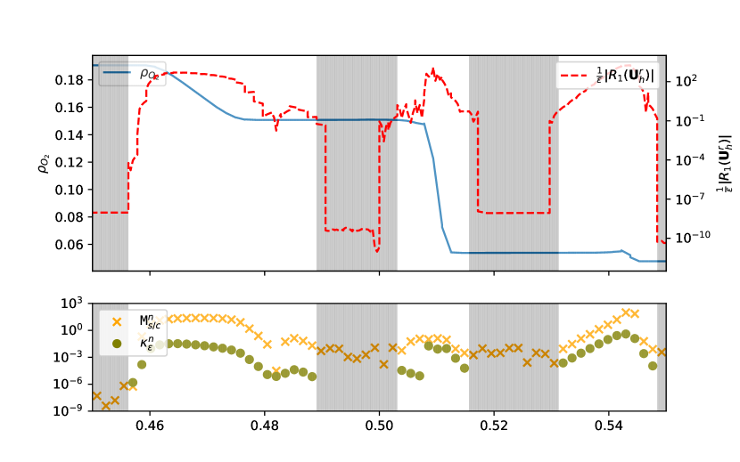
Figure 1: $t=4.375\cdot 10^{-4}$. Gray areas indicate $\Omega_{s}$, white background $\Omega_{c}$.

The initial discontinuity gives rise to a rarefaction wave, a shock and a contact discontinuity. After the first time step, the model adaptation strategy leads to the simple system being employed in regions where the solution is constant. In regions where the waves emerge due to the initial discontinuity the complex system is selected, see Figure 1.

As the contact discontinuity and the shock travels to the right and the rarefaction travels to the left, the numerical solution approaches equilibrium in the two plateaus between the three waves. As a result, the simple system is selected between the contact discontinuity and the shock from time $2.6125\cdot 10^{-4}$ onward, and between the rarefaction and the contact discontinuity from time $t=3.725\cdot 10^{-4}$ onward. The switch to the simple system is made once the modeling error indicator and the model coarsening distance are smaller than the prescribed tolerances and the number of cells in the patch where the simple system is to be employed in more than one cell.

The complex system has to be employed near the contact discontinuity, the shock and the rarefaction. In the case of the rarefaction, this is due to the fact that the rarefaction continues to expand as it travels to the left. Hence, the states that make up the rarefaction are away from the equilibrium manifold. In the case of the contact discontinuity and the shock, since the discontinuities are spread over a few cells, the states of the discontinuities are away from the equilibrium manifold as well. The size of the two patches of cells in between the emerged waves where the simple system is employed increases in the long run.

Thus, the model adaptation strategy leads to employment of the simple system, locally in time and space and does not result in undesirable back and forth switching between the two systems. The switch back to the complex system is only triggered if the number of cells in a patch where the simple system is employed falls below one. We can infer that the model adaptation strategy works well by ensuring that the numerical solution is close to the equilibrium manifold and ensuring that the dynamics is close to that of the equilibrium dynamics before switching to the simple system. This is also suggested by the fact that the source term in the reference simulations is of a smaller magnitude in the regions where the simple system is set.

References

• (1) Boscarino, S., Qiu, J., Russo, G., Xiong, T.: High order semi-implicit WENO schemes for all-mach full Euler system of gas dynamics. SIAM J. Sci. Comput. pp. 368–394 (2022)
• (2) Bothe, D., Dreyer, W.: Continuum thermodynamics of chemically reacting fluid mixtures. Acta Mech. 226, 1757–1805 (2015)
• (3) Chase, M.: NIST-JANAF Thermochemical Tables. American Institute of Physics (1998)
• (4) Cockburn, B., Shu, C.W.: The Runge Kutta Discontinuous Galerkin method for conservation laws V: Multidimensional systems. J. Comput. Phys. 141, 199–224 (1998)
• (5) Dafermos, C.: Hyperbolic Conservation Laws in Continuum Physics. Springer (2010)
• (6) Dedner, A., Giesselmann, J.: A posteriori analysis of fully discrete method of lines discontinuous Galerkin schemes for systems of conservation laws. SIAM J. Numer. Anal. 54, 3523–3549 (2016)
• (7) Gerhard, N., Iacono, F., May, G., Müller, S., Schäfer, R.: A high-order discontinuous Galerkin discretization with multiwavelet-based grid adaptation for compressible flows. J. Sci. Comput. 62, 25–52 (2015)
• (8) Gerhard, N., Müller, S., Sikstel, A.: A wavelet-free approach for multiresolution-based grid adaptation for conservation laws. Communications on Applied Mathematics and Computation 4, 1–35 (2021)
• (9) Giesselmann, J., Makridakis, C., Pryer, T.: A posteriori analysis of discontinuous Galerkin schemes for systems of hyberbolic conservation laws. SIAM J. Numer. Anal. 53, 1280–1303 (2015)
• (10) Giesselmann, J., Pryer, T.: A posteriori analysis for dynamic model adaptation problems in convection dominated problems. Math. Models Methods Appl. Sci. 27, 2381–2432 (2017)
• (11) Gnoffo, P., Gupta, R., Shinn, J.: Conservation equations and physical models for hypersonic air flows in thermal and chemical nonequilibrium. NASA TP (1989)
• (12) Gottlieb, S., Shu, C.W., Tadmor, E.: Strong stability-preserving high-order time discretization methods. SIAM Rev. 1, 89–112 (2001)
• (13) Joshi, H.: Mesh and model adaptation for hyperbolic balance laws. Ph.D. thesis, TU Darmstadt (2022)
• (14) Lide, D.: Handbook of Chemisty and Physics. CRC (2010)
• (15) Miroshnikov, A., Konstantina Trivisa: Relative entropy in hyperbolic relaxation for balance laws. Commun. Math. Sci 12, 1017–1043 (2014)
• (16) Müller, S., Sikstel, A.: Multiwave. https://www.igpm.rwth-aachen.de/forschung/multiwave, Institut für Geomtrie und Praktische Mathematik, RWTH Aachen (2018)
• (17) Pareschi, L., Russo, G.: Implicit-explicit Runge-Kutta schemes for stiff systems of differential equations. Adv. Theory Comput. Math. 3 (2001)
• (18) Pareschi, L., Russo, G.: Implicit-Explicit Runge-Kutta schemes and applications to hyperbolic systems with relaxation. J. Sci. Comput. 25, 129–155 (2007)
• (19) Tzavaras, A.: Relative entropy in hyperbolic relaxation. Commun. Math. Sci 3, 119–132 (2005)