Unification of popular artificial neural network activation functions

Abstract

We present a unified representation of the most popular neural network activation functions. Adopting Mittag-Leffler functions of fractional calculus, we propose a flexible and compact functional form that is able to interpolate between various activation functions and mitigate common problems in training neural networks such as vanishing and exploding gradients. The presented gated representation extends the scope of fixed-shape activation functions to their adaptive counterparts whose shape can be learnt from the training data. The derivatives of the proposed functional form can also be expressed in terms of Mittag-Leffler functions making it a suitable candidate for gradient-based backpropagation algorithms. By training multiple neural networks of different complexities on various datasets with different sizes, we demonstrate that adopting a unified gated representation of activation functions offers a promising and affordable alternative to individual built-in implementations of activation functions in conventional machine learning frameworks.

I Introduction

Activation functions are one of the key building blocks in artificial s that control the richness of the neural response and determine the accuracy, efficiency and performanceClevert et al. (2015) of multilayer neural networks as universal approximators.Hornik et al. (1989) Due to their biological linksAbbott and Dayan (2001); Haykin (1999) and optimization performance, saturating activation functionsGulcehre et al. (2016) such as logistic Sigmoid and hyperbolic tangent Costarelli and Spigler (2013) were commonly adopted in early neural networks. Nevertheless, both activation functions suffer from the vanishing gradient problem.Hochreiter (1998) Later studies on image classification using restricted Boltzmann machinessNair and Hinton (2010) and deep sGlorot et al. (2011) demonstrated that rectified linear units can mitigate the vanishing gradient problem and improve the performance of neural networks. Furthermore, the sparse coding produced by ReLUs not only creates a more robust and disentangled feature representation but also accelerates the learning process.Glorot et al. (2011)

The computational benefits and the current popularity of ReLUs should be taken with a grain of salt due to their notable disadvantages such as bias shift,Clevert et al. (2015) ill-conditioned parameter scalingGlorot et al. (2011) and dying ReLU.Lu et al. (2020) Furthermore, the unbounded nature of ReLUs for positive inputs, while potentially helpful for training deep s, can aggravate the exploding gradient problem in recurrent s.Bengio et al. (1994); Pascanu et al. (2013) In order to address the dying ReLU and the vanishing/exploding gradient problems, a multitude of ReLU variants have been proposedMaas et al. (2013); Qiu et al. (2017); Liu et al. (2019); He et al. (2015); Jin et al. (2015) but none has managed to consistently outperform the vanilla ReLUs in a wide range of experiments.Xu et al. (2015) Alternative activation functions such as exponential linear unitsClevert et al. (2015) and scaled sKlambauer et al. (2017) have also been proposed to build upon the benefits of ReLU and its variants and provide more robustness and resistance to the input noise. Yet, among the existing slew of activation functions in the literature,DasGupta and Schnitger (1992); Apicella et al. (2021); Duch and Jankowski (1999) no activation function seems to offer global superiority across all modalities and application domains.

Trainable activation functions,Chen and Chang (1996); Guarnieri et al. (1999); Piazza et al. (1993, 1992) whose functional form is learnt from the training data, offer a more flexible option than their fixed-shape counterparts. In order be able to fine-tune the shape of activation functions during backpropagation,Rumelhart et al. (1986) partial derivatives of activation functions with respect to unknown learning parameters are required. It is important to note that some trainable activation functions can also be replaced by simpler multilayer feed-forward subnetworks with constrained parameters and classical fixed-shape activation functions.Apicella et al. (2021) The ability to replace a trainable activation function with a simpler sub-neural network highlights a deep connection between the choice of activation functions and performance of neural networks. As such, pre-setting the best possible trainable activation function parameters or fine-tuning the experimental settingsSmith (2018) such as data preprocessing methods, gradient and weight clipping,Pascanu et al. (2013) optimizers,Polyak (1964); Nesterov (1983); Duchi et al. (2011); Hinton et al. (2012a); Kingma and Ba (2014) regularization methods such as $L_{1}$, $L_{2}$ and drop out,Hinton et al. (2012b) batch normalization (BN),Ioffe and Szegedy (2015) learning rate scheduling,Smith (2018); Senior et al. (2013) (mini-)batch size, or network designHagan et al. (2014) variables such as depth (number of layers) and width (number of neurons per layer) of the neural network as well as weight initialization methodsGlorot and Bengio (2010); He et al. (2015); Montavon et al. (2012) becomes an important but challenging task. Several strategies such as neural architecture searchLiu et al. (2018) and network design space designRadosavovic et al. (2020) have been proposed to assist the automation of the network designHagan et al. (2014) process but they have to deal with an insurmountable computational cost barrier for practical applications.

In this manuscript, we take a theoretical neuroscientific standpointAbbott and Dayan (2001) towards activation functions by emphasizing the existing connections among them from a mathematical perspective. As such, we resort to the expressive power of rational functions as well as higher transcendental special functions of fractional calculus to propose a unified gated representation of activation functions. The presented functional form is conformant with the outcome of a semi-automated search, performed by Ramachandran et al.,Ramachandran et al. (2017) in order to find the optimal functional form of activation functions over a pre-selected set of functions. The unification of activation functions offers several significant benefits: It requires fewer lines of code to be implemented and leads to less confusion in dealing with a wide variety of empirical guidelines on activation functions because individual activation functions correspond to special parameter sets in the gated representation. The proposed functional form is closed under differentiation making it a suitable choice for an efficient implementation of backpropagation algorithms commonly used for training ANNs. Finally, the unified functional can be adopted as a fixed-shape or trainable activation function or both when training neural networks. In other words, one can access different activation functions or interpolate between them by fixing or varying a set of parameters in the gated functional representation, respectively.

The manuscript is organized as follows: In Sec. II, we introduce Mittag-Leffler functions of one- and two-parameters and discuss their important analytical and numerical properties. Next, we use Mittag-Leffler functions to create a gated representation that can unify a set of most commonly used activation functions. Section III delineates the computational details of our experiments presented in Sec. IV, where we provide numerical evidence for the efficiency and accuracy of the proposed functional form. Concluding remarks and future directions are presented in Sec. V.

II Theory

II.1 Mittag-Leffler functions of one- and two-parameters

Mittag-Leffler functions, sometimes referred to as “the queen of functions in fractional calculus”,Mainardi and Gorenflo (2007); Mainardi (2020) are one of the most important higher transcendental functions that play a fundamental role in fractional calculus.Samko et al. (1993); Bǎleanu et al. (2019); Podlubny (1999) The interested reader is referred to Refs. 46, 48 and 49 for a survey of scientific and engineering applications. The one-parameter Mittag-Leffler function is defined asGorenflo et al. (2020); Kochubei and Luchko (2019)

$$E_{\alpha}(z)=\sum_{k=0}^{\infty}\frac{z^{k}}{\Gamma(\alpha k+1)},\qquad\alpha\in\mathbb{C},$$ (1)

where $\mathbb{C}$ denotes the set of complex numbers. For all values of $\operatorname{Re}(\alpha)>0$, the series in Eq. 1 converges everywhere in the complex plane and the one-parameter Mittag-Leffler function becomes an entire function of the complex variable $z$.Gorenflo et al. (2020) However, when $\operatorname{Re}(\alpha)<0$, the series in Eq. 1 diverges everywhere on $\mathbb{C}\ \!\backslash\ \!\{0\}$. As $\alpha\rightarrow 0^{+}$, the Mittag-Leffler function can be expressed asGorenflo et al. (2020)

$$E_{0}(\pm z)\sim\frac{1}{1\mp z},\qquad|z|<1.$$ (2)

Although Mittag-Leffler series has a finite radius of convergence, the restriction in Eq. 2 can be lifted and the asymptotic geometric series form can be adopted as a part of the definition of Mittag-Leffler function for $\alpha=0$Berberan-Santos (2005) The aforementioned definition seems to be consistent with the implementation of Mittag-Leffler function in Mathematica 13.2.Wolfram Research, Inc. Note that for $x>0$ and $0\leq\alpha\leq 1$, the one-parameter Mittag-Leffler function with negative arguments, $E_{\alpha}(-x)$, is a completely monotonicPollard (1948) function with no real zeros.Gorenflo et al. (2020)

The two-parameter Mittag-Leffler function can be similarly defined as

$$E_{\alpha,\beta}(z)=\sum_{k=0}^{\infty}\frac{z^{k}}{\Gamma(\alpha k+\beta)},\qquad\text{where}\quad\operatorname{Re}(\alpha)>0,\quad\text{and}\quad\beta\in\mathbb{C}.$$ (3)

The exponential form of Mittag-Leffler function, $E_{1}(z)=E_{1,1}(z)$, has no zeros in the complex plane. Nonetheless, for all $m\in\mathbb{N}$, where $\mathbb{N}$ is the set of natural numbers, $E_{1,-m}$ has its only $m+1$-order zero located at $z=0$. All zeros of $E_{2}(z)$ are simple and can be found on the negative real semi-axis. For a more detailed discussion on the distribution of zeros and the asymptotic properties of Mittag-Leffler functions, see Ref. 49.

Parallel to the study of analytic properties, the realization of accurate and efficient numerical methods for calculating Mittag-Leffler functions is still an open and active area of research.Karniadakis (2019); Gorenflo et al. (2020) In particular, the existence of free, open-source and accessible software for computing Mittag-Leffler functions is key to their usability in practical applications. We must note that the code base and programmatic details of recent updates to the implementation of Mittag-Leffler functions in Mathematica are not publicly available for further analysis in this manuscript. Nonetheless, several open-source modules for numerical computation of Mittag-Leffler functions are available in the public domain. Gorenflo et al.Gorenflo et al. (2002) have proposed an algorithm for computing two-parameter Mittag-Leffler functions that is suitable for use in Mathematica. Podlubny’s algorithm is implemented in MATLABThe MathWorks Inc. (2022) which allows the computation of Mittag-Leffler functions with arbitrary accuracy.Podlubny (2012) Garrappa has proposed an efficient method for calculating one- and two-parameter Mittag-Leffler functions using hyperbolic path integral transform and quadrature.Garrappa (2015a) Both MATLABGarrappa (2015b) and PythonHinsen (2017) implementations of Garrappa’s algorithm are also available in the public domain. Zeng and Chen have also constructed global Padé approximations for the special cases of parameters $0<\alpha\leq 1$ and $\beta\geq\alpha$, based on the complete monoticity of $E_{\alpha,\beta}(-x)$.Zeng and Chen (2015) Another powerful feature of Mittag-Leffler functions is their relation to other higher transcendental special functions such as hypergeometric, Wright, Meijer $G$ and Fox $H$-functionsGorenflo et al. (2020); Olver et al. (2010); Mathai and Saxena (1973); Abramowitz and Stegun (1964); Mathai et al. (2010) which allows for more general analytic and efficient numerical computations. For example, Mathematica automatically simplifies the one-parameter Mittag-Leffler functions with non-negative (half-)integer $\alpha$ to (sum of) generalized hypergeometric functions.Wolfram Research (2022a)

In addition to the algorithm complexity and implementation specifics, the total number of activation functions in a neural network can strongly affect its runtime on computing accelerators such as graphics processing units. The neural network architectureHagan et al. (2014) is also a major factor in determining the computational cost.Radosavovic et al. (2020) We will consider the impact of these factors in our numerical experiments in Sec. IV.

II.2 Gated representation of activation functions

In order to unify the most common classical fixed-shape activation functions, listed in a recent survey,Apicella et al. (2021) we propose the following functional form

$$x\Phi\biggl{[}x\biggl{|}\gamma\genfrac{.}{.}{0.0pt}{}{\alpha_{1}\ \beta_{1}\ f}{\alpha_{2}\ \beta_{2}\ g}\biggr{]}:=x\bigg{\{}x^{\gamma-1}\left(\frac{E_{\alpha_{1},\beta_{1}}\left[f(x)\right]}{E_{\alpha_{2},\beta_{2}}\left[g(x)\right]}\right)\bigg{\}},$$ (4)

where the gate function, $\Phi[f(x),g(x)]$, is a binary composition of two “well-behaved” functional mappings $f,g:\mathbb{R}\rightarrow\mathbb{R}$ and is responsible for generating a (non-)linear neural response. Here, $\mathbb{R}$ denotes the set of real numbers. The gated representation in Eq. 4 incorporates the functional form obtained from an automated search over a set of a pre-selected functionsRamachandran et al. (2017) and is consistent with the functional form of popular activation functions such as ReLU and Swish. Throughout this manuscript, we restrict ourselves to $\gamma\geq 0$, $\operatorname{Re}(\alpha)>0$ and $\beta\in\mathbb{R}$.

Table 1 presents a shortlist of popular fixed-shape classical activation functions that are accessible to the proposed gated representation as special cases via different sets of parameters.

Table 1: Special cases of gate function $\Phi$ in Eq. 4

Activation Function	Argument	$\gamma$	$\alpha_{1}$	$\alpha_{2}$	$\beta_{1}$	$\beta_{2}$	$f(x)$	$g(x)$
ReLUa	$x$	1	1	1	1	1	0	0
Sigmoid	$x$	0	0	1	1	1	$-e^{-x}$	0
Swish	$x$	1	0	1	1	1	$-e^{-cx}$	0
Softsign	$x$	1	0	1	1	1	$-|x|$	0
Hyperbolic Tangent	$x$	1	2	2	2	1	$x^{2}$	$x^{2}$
Mish	$\log(1+e^{x})$	2	2	2	2	1	$x^{2}$	$x^{2}$
Bipolar Sigmoidb	$x$	0	0	0	1	1	$-e^{-x}$	$e^{-x}$
	$x/2$	1	2	2	2	1	$x^{2}$	$x^{2}$
GELU	$x$	1	$1/2$	1	1	1	$x/\sqrt{2}$	$x^{2}/2$

• ^a The set of parameters are pertinent to $x\geq 0$, otherwise $\Phi=0$.

• ^b At least two representations exist for the Bipolar Sigmoid.

The ReLU is commonly represented in a piecewise functional form as $\max(0,x)$. In order to mimic this behavior, the gate function in Eq. 4 should reduce to identity for $x>0$ and zero otherwise. The former condition is satisfied when $\gamma=1$ and $E_{\alpha_{1},\beta_{1}}\left[f(x)\right]/E_{\alpha_{2},\beta_{2}}\left[g(x)\right]=1$, for which $\Phi\biggl{[}x\biggl{|}1\genfrac{.}{.}{0.0pt}{}{\alpha\ \beta\ f}{\alpha\ \beta\ f}\biggr{]}=1$ is the trivial case. Plots of ReLU activation function and its gated representation are shown in Fig. 1(a). Note that the y-axis label, $a(x)$, collectively refers to activation functions regardless of their functional form.

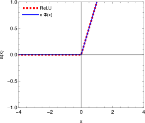
(a)

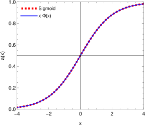
(b)

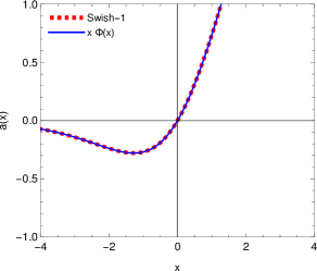
(c)

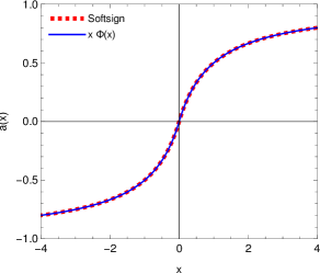
(d)

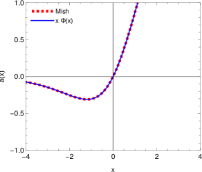
(e)

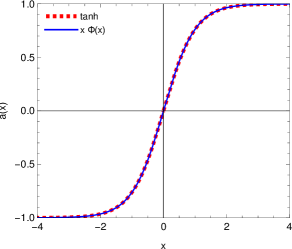
(f)

Figure 1: Plots of built-in and gated representation of various activation functions

The gate functional for Sigmoid activation function, $\sigma(x)$, takes $f(x)=-e^{-x}$ and $g(x)=0$ to yield

$$x\Phi\bigg{[}x\bigg{|}0\ \begin{matrix}0&1&-e^{-x}\\ 1&1&0\end{matrix}\bigg{]}=\frac{1}{1+e^{-x}}=\sigma(x).$$ (5)

Plots of Sigmoid activation function and its gated representation are shown in Fig. 1(b). The Sigmoid gate function in Eq. 5 can be morphed into that of Swish by setting $\gamma=1$ and $f(x)=e^{-cx}$ to obtain

$$x\Phi\bigg{[}x\bigg{|}1\ \begin{matrix}0&1&-e^{-cx}\\ 1&1&0\end{matrix}\bigg{]}=x\ \!\sigma(cx),$$ (6)

where $c$ is a trainable parameter. For $c=1$, the resulting activation function in Eq. 6 is referred to as Swish-1.Ramachandran et al. (2017) Plots of Swish-1 activation function and its gated variant are shown in Fig. 1(c). Setting $f(x)=-|x|$ in the gate function, one can convert Swish into Softsign, defined as

$$x\Phi\bigg{[}x\bigg{|}1\ \begin{matrix}0&1&-|x|\\ 1&1&0\end{matrix}\bigg{]}=\frac{x}{1+|x|}.$$ (7)

Plots of Softsign activation function and its gated representation are illustrated in Fig. 1(d). The gate functional for the hyperbolic tangent activation function takes $f(x)=g(x)=x^{2}$ to yield

$$x\Phi\bigg{[}x\bigg{|}1\ \begin{matrix}2&2&x^{2}\\ 2&1&x^{2}\end{matrix}\bigg{]}=\tanh(x).$$ (8)

Plots of hyperbolic tangent activation function and its gated representation are presented in Fig. 1(f). As mentioned in Sec. I, the gated functional form in Eq. 4 arms us with significant variational flexibility– In addition to accessing a set of fixed-shape activation functions via setting the gate function parameters, we can also interpolate between different functional forms by varying those parameters over a finite domain. Figure 2 illustrates an example where by fixing all parameters in the gated representation of hyperbolic tangent except $\beta_{2}$, one can smoothly interpolate between linear $(\beta_{2}=2)$ and hyperbolic tangent $(\beta_{2}=1)$ activation functions. Thus, it is possible to tune the saturation behavior of gated representation of saturating functions such as hyperbolic tangent and mitigate their vanishing/exploding gradient problem in a controlled fashion.Nair and Hinton (2010); Glorot and Bengio (2010); Glorot et al. (2011) Furthermore, one can turn $\beta_{2}$ (or in principle, any other parameter) into a trainable parameter and allow the hosting neural network to learn its optimal value from the training data.

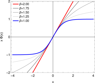
Figure 2: The interpolation of $x\Phi\biggl{[}x\biggl{|}1\genfrac{.}{.}{0.0pt}{}{2~{}2\ x^{2}}{2\ \beta\ x^{2}}\biggr{]}$ between linear and hyperbolic tangent functions

Our unification strategy can go beyond the aforementioned list of fixed-shape or trainable activation functions. For instance, MishMisra (2019) can be obtained by passing Softplus, $\log(1+e^{x})$, to hyperbolic tangent gate function as an argument and setting $\gamma=2$ to get

$$x\Phi\bigg{[}\log(1+e^{x})\bigg{|}2\ \begin{matrix}2&2&x^{2}\\ 2&1&x^{2}\end{matrix}\bigg{]}=x\ \!\tanh\big{[}\log(1+e^{x})\big{]}.$$ (9)

The Bipolar Sigmoid function can also be expressed by using the hyperbolic tangent gate function and passing a scaled linear function as an argument

$$x\Phi\bigg{[}\frac{x}{2}\bigg{|}1\ \begin{matrix}2&2&x^{2}\\ 2&1&x^{2}\end{matrix}\bigg{]}=\tanh\left(\frac{x}{2}\right).$$ (10)

Equivalently, one can also express the Bipolar Sigmoid function with a different set of paramenters and arguments in the gate function as

$$x\Phi\bigg{[}x\bigg{|}0\ \begin{matrix}0&1&-e^{-x}\\ 0&1&e^{-x}\end{matrix}\bigg{]}=\frac{1-e^{-x}}{1+e^{-x}}.$$ (11)

Setting $f(x)=\tfrac{x}{\sqrt{2}}$ and $g(x)=\tfrac{x^{2}}{2}$, the Gaussian error linear unit (GELU) activation function can also be written as

$$\frac{x}{2}\Phi\bigg{[}x\bigg{|}1\ \begin{matrix}\frac{1}{2}&1&\frac{x}{\sqrt{2}}\\ 1&1&\frac{x^{2}}{2}\end{matrix}\bigg{]}=\frac{x}{2}\bigg{[}1+\operatorname{erf}\left(\frac{x}{\sqrt{2}}\right)\bigg{]},$$ (12)

where $\operatorname{erf}(\cdot)$ is the error function.Abramowitz and Stegun (1964); Olver et al. (2010)

III Computational details

In order to compare the efficiency and performance of gated activation functions and their counterparts from Table 1, we design four sets of image classification experiments involving multiple neural network architectures and datasets of different sizes and complexities. In particular, we train the classical LeNet-5 neural networkLecun et al. (1998) on the Modified National Institute of Standards and Technology (MNIST)LeCun et al. (1998) and CIFAR-10Krizhevsky (2009) datasets as well as ShuffleNet-v2 and ResNet-101 neural networks on the ImageNet-1k dataset.Russakovsky et al. (2015)

The first two sets of experiments involve replacing all three element-wise ReLU activation functions in LeNet-5 architecture (Fig. 3) with their counterparts from Table 1. In each experiment, we run an ensemble of twenty independent sessions and train the LeNet-5 neural network on the MNIST and CIFAR-10 datasets for 10 and 20 epochs, respectively. In order to help the fairness of the comparisons between different experiments, we randomly initialize the network parameters using “1234” as a seed to ensure individual training sessions in each ensemble start with the same set of parameters. All training sessions are performed in-memory,Wolfram Research (2022b) with a batch size of 64 and in single-precision. The average results are rounded to four significant digits and reported in Tables 2 and 3.

In the next set of experiments, we replace the ReLU activation function in the ShuffleNet-v2’s terminal convolutional layer (Fig. 4) with its counterparts from Table 1. We also modify the ResNet-101 architecture by replacing a pair of ReLU activation functions in the last bottleneck block (Fig. 5) with various functions from Table 1. Each experiment is an ensemble of three independent sessions where we train the ShuffleNet-v2 and ResNet-101 neural networks on the ImageNet-1k dataset with batch sizes of 1024 and 128, respectively. He initializationHe et al. (2015) method and mixed precision are used for training both neural networks and the best average performance results presented in Tables 4 and 5, respectively. All training sessions pertinent to the ShuffleNet-v2 and ResNet-101 neural networks are performed out-of-core, in which batches of data are transferred to the neural network on the GPU on-the-fly.Wolfram Research (2022b) We stop the training when the absolute change in the macro-average value of F1-score falls below 0.001 for at least ten consecutive epochs.

The adaptive momentum (ADAM) optimizer is used for all training experiments with the stability parameter, the first and the second moment exponential decay rates set to $\epsilon=10^{-5}$, $\beta_{1}=0.9$ and $\beta_{2}=0.999$, respectively. The initial learning rate is set to 0.001 and automatically modified by the program. All computations are performed using Wolfram Mathematica 13.2.Wolfram Research, Inc. Bipolar Sigmoid and GELU are excluded from our studies as their hosting neural networks fail to converge without deviating from the selected default settings in Mathematica and further modifications to avoid the divergence. In this manuscript, we do not make any attempts to optimize the performance of the neural networks by fine-tuning various hyperparameters.

Three hardware platforms are adopted for performing the computations: a single laptop armed with a NVIDIA GeForce GTX 1650 GPU, a Supermicro workstation with 2 $\times$ NVIDIA A100 80GB PCIe GPUs and a NVIDIA DGX high-performance computing (HPC) cluster node with 8 $\times$ NVIDIA A100 80GB PCIe GPUs. The resulting data from the first setup can be found in the Supporting Information. The trajectory of all training instances are recorded in byte representation files that can be instantly reproduced in Mathematica. Furthermore, all input scripts and output logs alongside a simple Mathematica code snippet are also provided to assist the readers in reproducing the results.

IV Results and discussion

In order to quantify the impacts of various activation functions on the performance of LeNet-5, ShuffleNet-v2 and ResNet-101 classifiers during training and validation, we focus on a variety of numerical metrics such as loss, accuracy, precision, recall and F1-score. The training loss is measured via multi-class cross-entropy which is defined asWilmott (2019); Géron (2017)

$$\mathscr{L}=-\sum_{i=1}^{N}\sum_{k=1}^{K}y_{i,k}\ln(\hat{y}_{i,k}).$$ (13)

For each data point (image) $i$ in a dataset of size $N$, cross-entropy can measure how well the estimated probabilities, $\hat{y}_{i,k}$ for each class $k$, where $k\in\{1,2,3,\dots,K\}$, match those of the target class labels, $y_{i,k}$. Compared with other loss functions, cross-entropy can also improve the convergence rate of the optimization process in our study by aggressively penalizing the incorrect predictions and generating larger gradients.Géron (2017) Accuracy is defined as the fraction of the number of times that a classifier is correct in its predictions.Wilmott (2019) Since accuracy is not an appropriate metric for imbalanced datasets,Géron (2017) such as ImageNet-1k,Luccioni and Rolnick (2022) we also consider precision and recall as metrics for the classification task. Precision and recall are the ratios of the number of correctly predicted positive classes to the total number of instances that are predicted as or are indeed positive, respectively. In theory, we are interested in classifiers that have high precision and recall values. In practice, however, one adopts the harmonic mean of precision and recall (called F1-score) in order to take into account the tradeoff between the aforementioned two metrics. We report the macro-average values of precision, recall and F1-score for all studied multi-class classification tasks, notwithstanding our knowledge about the (im)balanced nature of the class distributions in MNIST, CIFAR-10 or ImageNet-1k datasets. We also consider training runtime and processing rate, as recommended by Ref. 76, to better reflect the effects of various activation functions on the computational cost and complexity of each neural network.

IV.1 Training LeNet-5 on MNIST dataset

The MNIST dataset consists of 60,000 training and 10,000 testing grayscale images of hand-written digits ($0,1,2,\dots,9$) that are normalized and centered to a 28$\times$28 fixed size. We pulled the MNIST dataset from the Wolfram Data RepositoryWolfram Research (2016). Individual training sessions (excluding that of the baseline) involve replacing all three element-wise ReLU activation layers in the LeNet-5 architecture (Fig. 3) with their counterparts from Table 1.

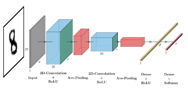
Figure 3: LeNet-5 neural network architecture

Table 2 shows the performance results for training/validation of LeNet-5 neural network on the MNIST dataset. For each activation function, there are two entries: the first entry refers to the results of built-in activation functions in Mathematica 13.2 and the second one corresponds to those of gated activation functions.

Table 2: The best performance metrics and timings pertinent to training and testing of LeNet-5 neural network on MNIST dataset with various activation functions^a

Activation Functionb	Loss	Accuracy (%)	Wall-Clock Time (s)
Sigmoid	0.0270 (0.0290)	99.13 (99.13)	21.93
	0.0270 (0.0290)	99.13 (99.13)	30.39
Swish-1	0.0411 (0.0295)	98.73 (98.98)	28.38
	0.0422 (0.0295)	98.69 (98.99)	30.60
Softsign	0.0138 (0.0324)	99.56 (99.00)	28.39
	0.0137 (0.0315)	99.56 (99.03)	28.61
$\tanh$	0.0146 (0.0329)	99.52 (98.95)	20.77
	0.0126 (0.0325)	99.58 (99.01)	29.72
Mish	0.0279 (0.0299)	99.14 (99.07)	24.38
	0.0339 (0.0304)	98.96 (99.03)	40.73
ReLUc	0.0144 (0.0292)	99.54 (99.16)	23.78

• ^a All results are ensemble averages over 20 independent training and testing experiments
          performed on a Supermicro workstation with NVIDIA A100 80GB PCIe GPUs.

• ^b The test results are given in parentheses. The first and second rows in each activation
          function entry correspond to the built-in and gated representations, respectively.

• ^c The LeNet-5 neural network architecture with ReLU activation functions is taken as
          baseline architecture.

Table 2 reveals that the average validation accuracy of LeNet-5 classifier on the MNIST test set is not significantly sensitive towards the choice of activation functions in the element-wise layers. In particular, the validation accuracy of LeNet-5 classifier armed with Sigmoid activation function is slightly smaller from that of the baseline neural network with ReLUs. Furthermore, choosing other activation functions such as Softsign and Mish seem to further deteriorate the corresponding average validation accuracies compared with that of ReLUs in the baseline LeNet-5 architecture. Plots of training/validation loss and accuracy versus epochs can be found in Supporting Information.

Our main interest in Table 2 is in the average values of total wall-clock time spent on training LeNet-5 on MNIST dataset using a Supermicro Workstation with NVIDIA A100 80GB PCIe GPUs. The average timings reveal that the added cost of calculating one- or two-parameter Mittag-Leffler functions in the gated representation of activation functions is small compared with their built-in variants implemented in Mathematica 13.2 program package.Wolfram Research (2022c) Specifically, the largest measured time gap is observed between the built-in and gated representations of Mish which mainly stems from the overhead of calculating Softplus and passing it as an argument to the two-parameter Mittag-Leffer function for each neural response in the element-wise activation layers. On the other hand, the computational time gap between built-in and gated representation of Softsign is very small on average.

IV.2 Training LeNet-5 on CIFAR-10 dataset

Table 3 presents the classification performance results for training/validation of LeNet-5 neural network on CIFAR-10 dataset which contains 50,000 training and 10,000 test images from 10 object classes (airplane, automobile, bird, cat, deer, dog, frog, horse, ship, and truck). Each data point in the CIFAR-10 dataset is a 32$\times$32 RGB image.Wolfram Research (2018)

Table 3: The best performance metrics and timings pertinent to training and testing of the LeNet-5 neural network on CIFAR-10 dataset with various activation functions^a

Activation Functionb	Loss	Accuracy (%)	Wall-Clock Time (s)
Sigmoid	0.7353 (1.0151)	74.79 (65.39)	44.26
	0.7353 (1.0152)	74.78 (65.38)	54.97
Swish-1	0.7323 (0.9016)	74.55 (69.39)	54.44
	0.7322 (0.9018)	74.55 (69.40)	60.77
Softsign	0.6380 (0.9297)	77.89 (68.64)	53.09
	0.6280 (0.9313)	78.26 (68.56)	54.52
$\tanh$	0.8129 (0.9766)	71.63 (66.79)	45.58
	0.8015 (0.9738)	72.05 (66.90)	56.09
Mish	0.6842 (0.8914)	76.18 (69.40)	48.37
	0.6841 (0.8913)	76.18 (69.44)	78.09
ReLUc	0.7299 (0.9279)	74.57 (68.24)	45.08

• ^a All results are ensemble averages over 20 independent training and testing experiments
          performed on a Supermicro workstation with NVIDIA A100 80GB PCIe GPUs.

• ^b The test results are given in parentheses. The first and second rows in each activation
          function entry correspond to the built-in and gated representations, respectively.

• ^c The LeNet-5 neural network architecture with ReLU activation functions is taken as
          baseline architecture.

All results correspond to the average of 20 individual training sessions, each running for 20 epochs. A comparison of the average accuracy values in Table 3 with those in Table 2 reflects the more intricate nature of the CIFAR-10 dataset which requires deeper neural networks, more advanced architectural design and training strategies. The interested reader is referred to a study on “Convolutional Deep Belief Neural Networks on CIFAR-10”Krizhevsky (2010) and ImageNet competition for a chronological survey of the efforts on this topic.Russakovsky et al. (2015) Table 3 reveals that the validation accuracy of LeNet-5 neural network can be improved by replacing ReLUs with any other activation function considered in this study with the exception of Sigmoid and hyperbolic tangent. In particular, replacing ReLUs with Swish-1 or Mish yields the largest improvement in the validation accuracy of approximately 1.2 %.

The average timings for training LeNet-5 neural network on CIFAR-10 dataset show similar trends to those presented in Table 2. Among all studied variants of the LeNet-5 architecture, those with built-in and gated Mish activation functions show the largest wall-clock time difference of approximately 30 seconds. Note that the timings in Table 3 are roughly twice their counterparts in Table 2 due to the adopted number of training epochs (20 for CIFAR-10 compared with 10 for MNIST). The average timings reported in both tables suggest that a unified implementation of the most popular activation functions using Mittag-Leffler functions is possible at an affordable computational cost compared with their individual built-in implementations. The gap between the built-in and gated representations of activation functions can be further reduced as more efficient algorithms and implementations of special functions such as Mittag-Leffler function become available. A comparison of the aforementioned timings obtained using a Supermicro workstation with NVIDIA A100 80GB PCIe GPUs (Tables 2 and 3) with those computed by a laptop with a NVIDIA GeForce GTX 1650 GPU (see Supporting Information) demonstrates that the availability of more powerful computing accelerators can also be an important factor for training ANNs with large numbers of gated activation functions.

IV.3 Training ShuffleNet-v2 on ImageNet-1k dataset

The ImageNet-1k dataset consists of 1,281,167 training, 50,000 validation and 100,000 test RGB images within 1000 categories.Russakovsky et al. (2015) All images are cropped and resized to 224$\times$224 pixels during preprocessing. Table 4 shows the performance results for training/validation of ShuffleNet-v2Ma et al. (2018) on the ImageNet-1k dataset where individual entries correspond to the ensemble average of three independent training experiments.

Table 4: The best performance metrics and timings for training and testing ShuffleNet-v2 neural network on the ImageNet-1k dataset using various activation functions^a

Activation Functionb	Loss	Accuracy	Precision	Recall	F1 Score	Processing Rate	Wall-Clock Time
		(%)	(%)	(%)	(%)	(images/s)	(h)
Sigmoid	0.8648 (1.923)	76.49 (59.55)	76.32 (62.24)	76.42 (59.55)	76.35 (59.41)	466	20.42
	0.8885 (1.919)	75.95 (59.33)	75.77 (62.02)	75.87 (59.33)	75.80 (59.16)	363	23.12
Swish-1	0.7114 (1.860)	80.36 (61.91)	80.25 (63.92)	80.32 (61.91)	80.27 (61.84)	437	17.63
	0.7113 (1.874)	80.37 (61.98)	80.26 (63.89)	80.32 (61.98)	80.28 (61.82)	348	20.44
SoftSign	0.7836 (1.845)	78.52 (60.96)	78.37 (63.13)	78.46 (60.96)	78.40 (60.84)	413	22.70
	0.8114 (1.823)	77.87 (60.92)	77.72 (62.99)	77.81 (60.92)	77.74 (60.72)	313	26.88
$\tanh$	0.8288 (1.882)	77.46 (60.53)	77.32 (62.73)	77.41 (60.53)	77.34 (60.35)	346	27.38
	0.8488 (1.867)	77.02 (60.50)	76.87 (62.78)	76.97 (60.50)	76.90 (60.33)	336	24.33
Mish	0.7545 (1.825)	79.37 (61.99)	79.25 (64.10)	79.32 (61.99)	79.27 (61.87)	307	26.48
	0.7057 (1.859)	80.47 (62.05)	80.35 (63.90)	80.41 (62.05)	80.37 (61.90)	360	24.22
ReLUc	0.7456 (1.669)	79.78 (63.50)	79.67 (64.80)	79.72 (63.50)	79.68 (63.33)	302	20.06

• ^a All results are ensemble averages over 3 independent training and testing experiments performed on a NVIDIA DGX
   HPC cluster node with NVIDIA A100 80GB PCIe GPUs.

• ^b The test results are given in parentheses. The first and second rows in each activation function entry correspond to
   the built-in and gated representations, respectively.

• ^c The ShuffleNet-v2 neural network (Ref. 76) with ReLU activation functions is taken as baseline architecture.

Each experiment involves replacing the ReLU activation function in the ShuffleNet-v2’s final convolutational layer (Fig. 4) with one of its counterparts from Table 1.

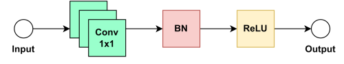
Figure 4: The final (target) convolution layer in the ShuffleNet-v2 architecture

Table 4 provides numerical evidence of overfitting where ShuffleNet-v2 performs significantly better in memorizing the training data than generalizing to the unseen data during validation (F1-score of 75-80% vs. 59-63%). The best validation loss and accuracy values are obtained by the ShuffleNet-v2 baseline architecture with ReLU activation functions. However, substituting the ReLU activation function with other variants from Table 1 deteriorates the validation loss and accuracy by at least 9% and 2%, respectively. Similar trends are observed for validation precision, recall and F-score macro-averages across Table 4 which also highlight the imbalanced nature of the ImageNet-1k datasetLuccioni and Rolnick (2022)– one of the main reasons behind choosing F1-score as our early stopping convergence criterion for training and performance metric for analysis. Table 4 demonstrates that the top three performers based on validation F1-score are the ShuffleNet-v2 neural networks with ReLU (63.3%), Mish (61.9%), and Swish-1 (61.8%) activation functions, respectively.

The performance results presented in Table 4 can also be impacted by system-dependent factors such as out-of-core data transfer bandwidth, core affinity, task binding and distribution over sockets, etc., commonly encountered in shared HPC cluster environments.Ma et al. (2018) As such, we complement our data in Table 4 with two additional temporal metrics to quantify the efficiency of ShuffleNet-v2 neural network with various activation functions: the total wall-clock runtime and processing rate. The availability of 80GB of GPU memory allowed us to adopt larger batch sizes (1024 vs. 4 images/batch) to facilitate achieving higher processing rates (approximately, 470 images/s) during training compared with those reported in Ref. 76 (190 images/s). Nonetheless, Table 4 illustrates that the processing rates of gated activation functions are in general lower than their built-in counterparts due to higher memory access costs and computational complexity. An exception is gated Mish activation function which is 53 images/s faster than its built-in variant. Notably, the processing rate of training ShuffleNet-v2 with built-in hyperbolic tangent is only 10 images/s faster than that of its gated counterpart. Both observations are corroborated by shorter total training wall-clock runtimes for gated Mish and hyperbolic tangent functions compared with those of their built-in variants. Furthermore, training ShuffleNet-v2 with Sigmoid and SoftSign activation functions show the largest differences in processing rates (of about 100 images/s) between their built-in and gated variants. The highest processing rates, however, are obtained by the built-in variants of Sigmoid (466 images/s), Swish-1 (437 images/s) and SoftSign (413 images/s) activation functions, respectively. The minimum average runtime of 17 hours is measured for training ShuffleNet-v2 neural network with built-in Swish-1 activation function which is approximately 3 hours shorter than those required by ReLU, built-in Sigmoid or gated Swish-1 activation functions.

IV.4 Training ResNet-101 on ImageNet-1k dataset

The performance results of training/validation of ResNet-101He et al. (2016) on the ImageNet-1k dataset are shown in Table 5 where each entry corresponds to the average of three independent training sessions.

Table 5: The best performance metrics and timings for training and testing ResNet-101 neural network on the ImageNet-1k dataset using various activation functions^a

Activation Functionb	Loss	Accuracy	Precision	Recall	F1 Score	Processing Rate	Wall-Clock Time
		(%)	(%)	(%)	(%)	(images/s)	(d)
Sigmoid	0.0700 (2.120)	98.08 (67.57)	98.08 (68.71)	98.07 (67.57)	98.07 (67.40)	143	3.1
	0.1268 (1.937)	96.34 (67.45)	96.34 (68.65)	96.33 (67.29)	96.33 (67.29)	82	4.6
Swish-1	0.0637 (2.118)	98.28 (67.76)	98.28 (68.90)	98.28 (67.76)	98.28 (67.60)	89	4.8
	0.0412 (2.382)	98.81 (67.82)	98.81 (68.79)	98.81 (67.82)	98.81 (67.66)	92d	8.3d
SoftSign	0.1691 (1.832)	95.16 (67.47)	95.14 (68.81)	95.14 (67.47)	95.14 (67.33)	140	2.5
	0.1710 (1.791)	95.07 (67.39)	95.06 (68.71)	95.06 (67.39)	95.06 (67.27)	82	4.2
$\tanh$	0.0632 (2.181)	98.26 (67.82)	98.25 (68.66)	98.25 (67.82)	98.25 (67.58)	95	5.8
	0.2184 (1.714)	93.75 (67.26)	93.73 (68.62)	93.73 (67.26)	93.73 (67.10)	77	3.0
Mish	0.0382 (2.450)	98.88 (68.02)	98.88 (68.89)	98.88 (68.02)	98.88 (67.76)	103d	8.2d
	0.0741 (2.103)	97.96 (67.79)	97.95 (68.80)	97.95 (67.79)	97.95 (67.61)	81	5.6
ReLUc	0.0689 (2.121)	98.14 (67.84)	98.14 (68.92)	98.13 (67.84)	98.13 (67.69)	86	5.7

• ^a All results are ensemble averages over 3 independent training and testing experiments performed on a NVIDIA DGX
   HPC cluster node with NVIDIA A100 80GB PCIe GPUs.

• ^b The test results are given in parentheses. The first and second rows in each activation function entry correspond to
   the built-in and gated representations, respectively.

• ^c The ResNet-101 architecture (Ref. 81) with the terminal bottleneck block of Fig. 5 is taken as baseline architecture.

• ^d Restarted trainings affected by the runtime limitations on the cluster node.

Individual training sessions involve replacing the first two ReLU activation functions in the final convolutional bottleneck block of the ResNet-101 baseline architecture (Fig. 5) with one of their counterparts from Table 1.

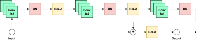
Figure 5: The bottleneck design with an identity shortcut in the ResNet-101 architecture

The performance results in Table 5 suggest that, similar to ShuffleNet-v2, the ResNet-101 neural network also overfits the ImageNet-1k data. Choosing different activation functions in ResNet101’s baseline architecture does not significantly change the value of validation performance metrics (i.e., accuracy, precision, recall and F1-score) with the exception of loss. In particular, variants of ResNet-101 neural network with gated hyperbolic tangent and vanilla Mish show the best validation loss (1.714) and accuracy (68.02%), respectively. Substituting the ReLU activation functions in the ResNet-101’s baseline architecture with any of their counterparts from Table 1 slightly deteriorates the validation precision and recall macro-averages with the exception of built-in Mish which improves the validation recall by less than 1%. The aforementioned improvement in the validation recall is also reflected in the value of F1-score corresponding to vanilla Mish (67.76%) compared with that of ResNet-101’s baseline architecture (67.69%).

Due to the runtime limitations on our HPC node, we had to restart our computations during training ResNet-101 with gated Swish-1 and built-in Mish activation functions. As such, we expect that the reported values for processing rates and wall-clock times for the two aforementioned cases to be affected by the disruption. Comparing the processing times in Table 5 with those in Table 4 reveals that the processing times corresponding to ShuffleNet-v2 are much higher than those of ResNet-101 which is consistent with the previous reports in literature.Ma et al. (2018) However, care must be taken as the adopted batch sizes for the two training sets are quite different (1024 for ShuffleNet-v2 vs. 128 for ResNet-101). The highest processing rates (of approximately 140 images/s) correspond to the ResNet-101 neural networks armed with built-in Sigmoid and SoftSign activation functions. The shortest training runtime is around 2 days which belongs to the ResNet-101 neural network with built-in SoftSign activation function. In comparison, the total training runtime corresponding to the baseline ResNet-101 architecture is longer by approximately 3 days.

V Conclusion and future work

In this manuscript, we have presented a unified representation of some of the most popular neural network activation functions of fixed-shape type. The proposed functional form not only sheds light on the direct analytical connections between several well-established activation functions in the literature but also allows for interpolating between different functional forms through varying the gate function parameters. The derivative of the gated activation function, defined in terms of Mittag-Leffler functions, is closed under differentiation. This characteristic of gated representations makes them a suitable candidate for training neural networks through gradient-based methods of optimization. A unified representation of activation functions is also beneficial to studies which use fixed-shape or trainable activation functions as it can lead to large savings in terms of number of code lines compared to what is otherwise required for individual implementation of activation functions in popular machine learning frameworks via inheritance and/or customized classes. Through training the classic LeNet-5, ShuffleNet-v2 and ResNet-101 neural networks on standard benchmark datasets such as MNIST, CIFAR-10, and ImageNet-1k, we have established that a unified implementation of activation functions is possible without any sacrifice in validation performance and at an affordable computational cost. The use of one- and two-parameter Mittag-Leffler functions and their relation to other generalized and special functionsOlver et al. (2010) such as hypergeometric and Wright functionsMainardi (2020) opens a door to a new and active area of research in fractional ANN and backpropagation algorithms which is also under current investigation by us.

Appendix

.1 General formula for derivatives of Mittag-Leffler function

The differentials of the one- and two-parameter Mittag-Leffler Functions can be expressed in terms of Mittag-Leffler function itself. The aforementioned closeness property is computationally beneficial for an efficient implementation of the gradient descent-based backpropagation algorithms for training ANNs. For a more in-depth discussion on differential and recurrence relations of Mittag-Leffler functions of one-, two- and three-parameter(s), see Refs. 49; 82.

Let $p\in\mathbb{N}$, where $\mathbb{N}$ denotes the set of natural numbers. Then, the general derivatives of one-parameter Mittag-Leffler function can be given as

$$\begin{gathered}\frac{d^{\ \!\!p}}{dz^{p}}E_{p}(z^{p})=E_{p}(z^{p}),\qquad\text{and}\\ \frac{d^{\ \!\!p}}{dz^{p}}E_{p/q}(z^{p/q})=E_{p/q}(z^{p/q})+\sum_{k=1}^{q-1}\frac{z^{-k/q}}{\Gamma(1-k/q)}\qquad q=2,3,\dots.\end{gathered}$$ (14)

Assuming $\alpha>0$ and $\beta\in\beta$, the first-derivative of the two-parameter Mittag-Leffler functions can be written as a sum of two instances of two-parameter Mittag-Leffler functions asGarrappa and Popolizio (2018)

$$\frac{d}{dz}E_{\alpha,\beta}(z)=\frac{E_{\alpha,\alpha+\beta-1}(z)+(1-\beta)E_{\alpha,\alpha+\beta}(z)}{\alpha}.$$ (15)

In general, one can write

$$\frac{d^{\ \!\!m}}{dz^{m}}E_{\alpha,\beta}(z)=\frac{1}{\alpha^{m}}\sum_{k=0}^{m}c^{(m)}_{k}E_{\alpha,\alpha m+\beta-k}(z),\qquad m\in\mathbb{N}$$ (16)

where the $c_{0}^{(0)}=1$ and the remaining coefficients for $k=0,1,2,\dots$ can be computed using the following recurrence relation

$$c_{k}^{(m)}=\begin{cases}\left[1-\beta-\alpha(m-1)\right]c_{0}^{(m-1)},\qquad k=0,\\ c_{k-1}^{(m-1)}+\left[1-\beta-\alpha(m-1)+k\right]c_{k}^{(m-1)},\qquad 1\leq k\leq m-1,\\ 1,\qquad k=m.\end{cases}$$ (17)

References

References

- Clevert et al. (2015) D. A. Clevert, T. Unterthiner, and S. Hochreiter, 4th International Conference on Learning Representations, ICLR 2016 - Conference Track Proceedings (2015), 10.48550/arxiv.1511.07289.
- Hornik et al. (1989) K. Hornik, M. Stinchcombe, and H. White, Neural Networks 2, 359 (1989).
- Abbott and Dayan (2001) L. F. Abbott and P. Dayan, Theoretical Neuroscience Computational and Mathematical Modeling of Neural Systems (MIT Press, 2001).
- Haykin (1999) S. Haykin, Neural Networks: A Comprehensive Foundation (2nd Edition) (Prentice-Hall, Inc., Upper Saddle River, New Jersey, USA, 1999).
- Gulcehre et al. (2016) C. Gulcehre, M. Moczulski, M. Denil, and Y. Bengio, 33rd International Conference on Machine Learning, ICML 2016 6, 4457 (2016).
- Costarelli and Spigler (2013) D. Costarelli and R. Spigler, Neural Networks 48, 72 (2013).
- Hochreiter (1998) S. Hochreiter, International Journal of Uncertainty, Fuzziness and Knowledge-Based Systems 6, 107 (1998).
- Nair and Hinton (2010) V. Nair and G. E. Hinton, in Proceedings of the 27th International Conference on International Conference on Machine Learning, ICML’10 (Omnipress, Madison, WI, USA, 2010) pp. 807–814.
- Glorot et al. (2011) X. Glorot, A. Bordes, and Y. Bengio, in International Conference on Artificial Intelligence and Statistics, Vol. 15 (2011) pp. 315–323.
- Lu et al. (2020) L. Lu, Y. Shin, Y. Su, and G. Em Karniadakis, Communications in Computational Physics 28, 1671 (2020).
- Bengio et al. (1994) Y. Bengio, P. Simard, and P. Frasconi, IEEE Transactions on Neural Networks 5, 157 (1994).
- Pascanu et al. (2013) R. Pascanu, T. Mikolov, and Y. Bengio, in Proceedings of the 30th International Conference on International Conference on Machine Learning - Volume 28, ICML’13 (JMLR, 2013) pp. 1310–1318.
- Maas et al. (2013) A. L. Maas, A. Y. Hannun, and A. Y. Ng, in Proceedings of the Thirteenth International Conference on Machine Learning, Vol. 28 (JMLR, Atlanta, Georgia, USA, 2013).
- Qiu et al. (2017) S. Qiu, X. Xu, and B. Cai, arXiv (2017), 10.48550/arxiv.1706.08098.
- Liu et al. (2019) Y. Liu, J. Zhang, C. Gao, J. Qu, and L. Ji, arXiv (2019), 10.48550/arxiv.1908.03682.
- He et al. (2015) K. He, X. Zhang, S. Ren, and J. Sun, in 2015 IEEE International Conference on Computer Vision (ICCV) (2015) pp. 1026–1034.
- Jin et al. (2015) X. Jin, C. Xu, J. Feng, Y. Wei, J. Xiong, and S. Yan, arXiv (2015), 10.48550/arXiv.1512.07030.
- Xu et al. (2015) B. Xu, N. Wang, H. Kong, T. Chen, and M. Li, (2015), 10.48550/arxiv.1505.00853.
- Klambauer et al. (2017) G. Klambauer, T. Unterthiner, A. Mayr, and S. Hochreiter, Advances in Neural Information Processing Systems 2017-December, 972 (2017).
- DasGupta and Schnitger (1992) B. DasGupta and G. Schnitger, in Advances in Neural Information Processing Systems, Vol. 5, edited by S. Hanson, J. Cowan, and C. Giles (Morgan-Kaufmann, 1992) pp. 615–622.
- Apicella et al. (2021) A. Apicella, F. Donnarumma, F. Isgrò, and R. Prevete, Neural Networks 138, 14 (2021).
- Duch and Jankowski (1999) W. Duch and N. Jankowski, Neural Computing Surverys 2, 163 (1999).
- Chen and Chang (1996) C. T. Chen and W. D. Chang, Neural Networks 9, 627 (1996).
- Guarnieri et al. (1999) S. Guarnieri, F. Piazza, and A. Uncini, IEEE Trans. Neural Networks 10, 672 (1999).
- Piazza et al. (1993) F. Piazza, A. Uncini, and M. Zenobi, Proceedings of the International Joint Conference on Neural Networks 2, 1401 (1993).
- Piazza et al. (1992) F. Piazza, A. Uncini, and M. Zenobi, Proc. of the IJCNN 2, 343 (1992).
- Rumelhart et al. (1986) D. E. Rumelhart, G. E. Hinton, and R. J. Williams, Nature 1986 323:6088 323, 533 (1986).
- Smith (2018) L. N. Smith, arXiv (2018), 10.48550/arxiv.1803.09820.
- Polyak (1964) B. T. Polyak, USSR Computational Mathematics and Mathematical Physics 4, 1 (1964).
- Nesterov (1983) Y. Nesterov, Doklady AN USSR 269, 543 (1983).
- Duchi et al. (2011) J. Duchi, E. Hazan, and Y. Singer, Journal of Machine Learning Research 12, 2121 (2011).
- Hinton et al. (2012a) G. Hinton, N. Srivastava, K. Swersky, and T. Tieleman, “Neural Networks for Machine Learning: Lecture 6a, Slide 29,” http://www.cs.toronto.edu/~hinton/coursera/lecture6/lec6.pdf (2012a), Last accessed on: 01/19/2023.
- Kingma and Ba (2014) D. P. Kingma and J. Ba, arXiv (2014), 10.48550/arxiv.1412.6980.
- Hinton et al. (2012b) G. E. Hinton, N. Srivastava, A. Krizhevsky, I. Sutskever, and R. R. Salakhutdinov, (2012b), 10.48550/arxiv.1207.0580.
- Ioffe and Szegedy (2015) S. Ioffe and C. Szegedy, in Proceedings of the 32nd International Conference on Machine Learning, Proceedings of Machine Learning Research, Vol. 37, edited by F. Bach and D. Blei (PMLR, Lille, France, 2015) pp. 448–456.
- Senior et al. (2013) A. Senior, G. Heigold, M. Ranzato, and K. Yang, ICASSP, IEEE International Conference on Acoustics, Speech and Signal Processing - Proceedings , 6724 (2013).
- Hagan et al. (2014) M. T. Hagan, H. B. Demuth, M. H. Beale, and O. De Jesús, Neural network design, 2nd ed. (https://hagan.okstate.edu/nnd.html, Middletown, Delaware, USA, 2014).
- Glorot and Bengio (2010) X. Glorot and Y. Bengio, in Proceedings of the Thirteenth International Conference on Artificial Intelligence and Statistics, Proceedings of Machine Learning Research, Vol. 9, edited by Y. W. Teh and M. Titterington (PMLR, Chia Laguna Resort, Sardinia, Italy, 2010) pp. 249–256.
- Montavon et al. (2012) G. Montavon, G. B. Orr, and K.-R. Müller, eds., Neural Networks: Tricks of the Trade, Lecture Notes in Computer Science, Vol. 7700 (Springer Berlin Heidelberg, Berlin, Heidelberg, 2012).
- Liu et al. (2018) H. Liu, K. Simonyan, and Y. Yang, arXiv (2018), 10.48550/arxiv.1806.09055.
- Radosavovic et al. (2020) I. Radosavovic, R. P. Kosaraju, R. Girshick, K. He, and P. Dollár, arXiv (2020), 10.48550/arxiv.2003.13678.
- Ramachandran et al. (2017) P. Ramachandran, B. Zoph, and Q. V. Le, arXiv (2017), 10.48550/arxiv.1710.05941.
- Mainardi and Gorenflo (2007) F. Mainardi and R. Gorenflo, Fractional Calculus and Applied Analysis 10, 269 (2007).
- Mainardi (2020) F. Mainardi, Entropy 22, 1359 (2020).
- Samko et al. (1993) S. Samko, A. A. Kilbas, and O. I. Marichev, Fractional integrals and derivatives: Theory and applications (Gordon and Breach Science Publishers, Amsterdam, 1993).
- Bǎleanu et al. (2019) D. Bǎleanu, A. Mendes Lopes, I. Petráš, V. E. Tarasov, G. E. Karniadakis, A. Kochubei, and Y. Luchko, eds., Handbook of fractional calculus with applications, Vol. 1–8 (De Gruyter, Berlin, Boston, 2019).
- Podlubny (1999) I. Podlubny, ed., Fractional differential equations: An introduction to fractional derivatives, fractional differential equations, to methods of their solution and some of their applications, Vol. 198 (Elsevier, 1999).
- Herrmann (2018) R. Herrmann, Fractional calculus: An introduction for physicists, 3rd ed. (World Scientific, 2018).
- Gorenflo et al. (2020) R. Gorenflo, A. A. Kilbas, F. Mainardi, and S. Rogosin, Mittag-Leffler Functions, Related Topics and Applications, 2nd ed., Springer Monographs in Mathematics (Springer Berlin Heidelberg, Berlin, Heidelberg, 2020).
- Kochubei and Luchko (2019) A. Kochubei and Y. Luchko, eds., Handbook of fractional calculus with applications: Basic theory, Vol. 1 (De Gruyter, 2019).
- Berberan-Santos (2005) M. N. Berberan-Santos, Journal of Mathematical Chemistry 38, 265 (2005).
- (52) Wolfram Research, Inc., “Mathematica, Version 13.2,” Champaign, IL, 2022.
- Pollard (1948) H. Pollard, Bulletin of the American Mathematical Society 54, 1115 (1948).
- Karniadakis (2019) G. E. Karniadakis, ed., Handbook of fractional calculus with applications: Numerical methods, Vol. 3 (De Gruyter, Berlin, Boston, 2019).
- Gorenflo et al. (2002) R. Gorenflo, J. Loutchko, and Y. Luchko, Fractional Calculus and Applied Analysis 5, 491 (2002).
- The MathWorks Inc. (2022) The MathWorks Inc., “MATLAB version: 9.13.0 (R2022b),” (2022).
- Podlubny (2012) I. Podlubny, “Mittag-Leffler function,” https://www.mathworks.com/matlabcentral/fileexchange/8738-mittag-leffler-function (2012), Version 1.2.0.0; Last accessed on: 01/08/2023.
- Garrappa (2015a) R. Garrappa, SIAM Journal of Numerical Analysis 53, 1350 (2015a).
- Garrappa (2015b) R. Garrappa, “The Mittag-Leffler function,” https://www.mathworks.com/matlabcentral/fileexchange/48154-the-mittag-leffler-function (2015b), Version 1.3.0.0; Last accessed on: 01/08/2023.
- Hinsen (2017) K. Hinsen, “The mittag-leffler function in python,” https://github.com/khinsen/mittag-leffler (2017), Last accessed on: 01/08/2023.
- Zeng and Chen (2015) C. Zeng and Y. Q. Chen, Fractional Calculus and Applied Analysis 18, 1492 (2015).
- Olver et al. (2010) F. Olver, D. Lozier, R. Boisvert, and C. Clark, The NIST Handbook of Mathematical Functions (Cambridge University Press, New York, NY, 2010).
- Mathai and Saxena (1973) A. M. Mathai and R. K. Saxena, Generalized Hypergeometric Functions with Applications in Statistics and Physical Sciences, Lecture Notes in Mathematics, Vol. 348 (Springer Berlin Heidelberg, Berlin, Heidelberg, 1973).
- Abramowitz and Stegun (1964) M. Abramowitz and I. A. Stegun, Handbook of Mathematical Functions with Formulas, Graphs, and Mathematical Tables (Dover, New York, USA, 1964).
- Mathai et al. (2010) A. M. Mathai, R. K. Saxena, and H. J. Haubold, The H-Function: Theory and Applications (Springer New York, 2010).
- Wolfram Research (2022a) Wolfram Research, “MittagLefflerE,” https://reference.wolfram.com/language/ref/MittagLefflerE.html (2022a), Last Accessed on: 2/20/2023.
- Misra (2019) D. Misra, (2019), 10.48550/arxiv.1908.08681.
- Lecun et al. (1998) Y. Lecun, L. Bottou, Y. Bengio, and P. Haffner, Proceedings of the IEEE 86, 2278 (1998).
- LeCun et al. (1998) Y. LeCun, C. Cortes, and C. J. Burges, “The MNIST Database of Handwritten Digits,” http://yann.lecun.com/exdb/mnist (1998), New York, USA.
- Krizhevsky (2009) A. Krizhevsky, “Learning Multiple Layers of Features from Tiny Images,” https://www.cs.toronto.edu/~kriz/cifar.html (2009).
- Russakovsky et al. (2015) O. Russakovsky, J. Deng, H. Su, J. Krause, S. Satheesh, S. Ma, Z. Huang, A. Karpathy, A. Khosla, M. Bernstein, A. C. Berg, and L. Fei-Fei, International Journal of Computer Vision (IJCV) 115, 211 (2015).
- Wolfram Research (2022b) Wolfram Research, “Training on Large Datasets,” https://reference.wolfram.com/language/tutorial/NeuralNetworksLargeDatasets.html (2022b), Last Accessed on: 7/16/2023.
- Wilmott (2019) P. Wilmott, Machine Learning : An Applied Mathematics Introduction (Panda Ohana Publishing, Oxford, United Kingdom, 2019).
- Géron (2017) A. Géron, Hands-on machine learning with Scikit-Learn and TensorFlow : concepts, tools, and techniques to build intelligent systems (O’Reilly Media, Sebastopol, CA, 2017).
- Luccioni and Rolnick (2022) A. S. Luccioni and D. Rolnick, arXiv 2208.11695 (2022).
- Ma et al. (2018) N. Ma, X. Zhang, H.-T. Zheng, and J. Sun, Computer Vision – ECCV 2018, edited by V. Ferrari, M. Hebert, C. Sminchisescu, and Y. Weiss (Springer International Publishing, Cham, 2018) pp. 122–138.
- Wolfram Research (2016) Wolfram Research, “”MNIST” from the Wolfram Data Repository,” https://doi.org/10.24097/wolfram.62081.data (2016), Last accessed on: 02/4/2023.
- Wolfram Research (2022c) Wolfram Research, “ElementwiseLayer,” https://reference.wolfram.com/language/ref/ElementwiseLayer.html (2022c), Last Accessed on: 2/19/2023.
- Wolfram Research (2018) Wolfram Research, “”CIFAR-10” from the Wolfram Data Repository ,” https://doi.org/10.24097/wolfram.83212.data (2018), Last accessed on: 02/6/2023.
- Krizhevsky (2010) A. Krizhevsky, “Convolutional Deep Belief Networks on CIFAR-10,” https://www.cs.toronto.edu/ kriz/conv-cifar10-aug2010.pdf (2010), Last accessed on: 02/11/2023.
- He et al. (2016) K. He, X. Zhang, S. Ren, and J. Sun, 2016 IEEE Conference on Computer Vision and Pattern Recognition (CVPR) , 770 (2016).
- Garrappa and Popolizio (2018) R. Garrappa and M. Popolizio, Journal of Scientific Computing 77, 129 (2018).