Active Galactic Nuclei with High-Resolution X-ray Spectroscopy

Abstract

The imminent launch of XRISM will usher in an era of high-resolution X-ray spectroscopy. For active galactic nuclei (AGN) this is an exciting epoch that is full of massive potential for uncovering the ins and outs of supermassive black hole accretion. In this work, we review AGN research topics that are certain to advance in the coming years with XRISM and prognosticate the possibilities with Athena and Arcus. Specifically, our discussion focuses on: (i) the relatively slow moving ionised winds known as warm absorbers and obscurers; (ii) the iron emitting from different regions of the inner and outer disc, broad line region, and torus; and (iii) the ultrafast outflows that may be the key to understanding AGN feedback.

0.1 Introduction

Active galactic nuclei (AGN) are unlike any other class of astronomical object. They cannot be described by a single, dominating process. Instead, AGN radiate energy over the entire electromagnetic spectrum, and are the sites of pair-production, cosmic rays, and gravitational waves. Radiation is created through multiple processes, including blackbody, synchrotron, Comptonisation, bremsstrahlung, and line emission. Gravity attracts material inward toward the black hole, but mass and energy can also be ejected into the host galaxy and beyond. Gas can be viewed in absorption and emission, and it exists in various physical states that can be optically thick and thin, as well as neutral and completely ionised. Ionisation (see Eq. 4) can occur through collisional and radiative excitation. Moreover, all these physical processes are subject to extreme gravity and magnetic fields, often invoking special and general relativity and relativistic magnetohydrodynamics (MHD). Researchers must draw from many areas of physics to understand AGN.

Though fascinating in their own right, AGN have far-reaching influence in other fields of astronomy. The AGN system is tiny in comparison to the host galaxy mass ($M_{BH}/M_{gal}\sim 0.001$; e.g. FM00 ; Gebhardt00 ), but its rest mass energy is comparable to the gravitational binding energy of the host galaxy. If a small fraction of the SMBH energy is deposited into the host galaxy or intracluster medium, this AGN feedback will influence how galaxies evolve. AGN feedback (e.g. Begelman04 ; King10 ; Fabian12 ) will be important if the kinetic luminosity

$$L_{KE}=\frac{1}{2}\dot{M}_{out}v_{r}^{2}$$ (1)

of the wind deposits into the host galaxy approximately $0.5\%-5\%$ of the AGN bolometric luminosity ($L_{bol}$) SR98 ; DiMatteo05 ; SH05 ; HE10 ; KP15 . In the kinetic luminosity expression (Eq. 1), $v_{r}$ is the radial velocity of the wind and

$$\dot{M}_{out}=\mu N_{H}m_{p}\Omega rfv_{r}$$ (2)

is the mass outflow rate in terms of the total column density ($N_{H}$), solid angle subtended by the outflow ($\Omega$), distance from the black hole ($r$), proton mass ($m_{p}$), the volume filling factor ($f$), $v_{r}$, and the mean atomic weight correction ($\mu$), which is $\sim 1.23$ for cosmic abundances blustin05 .

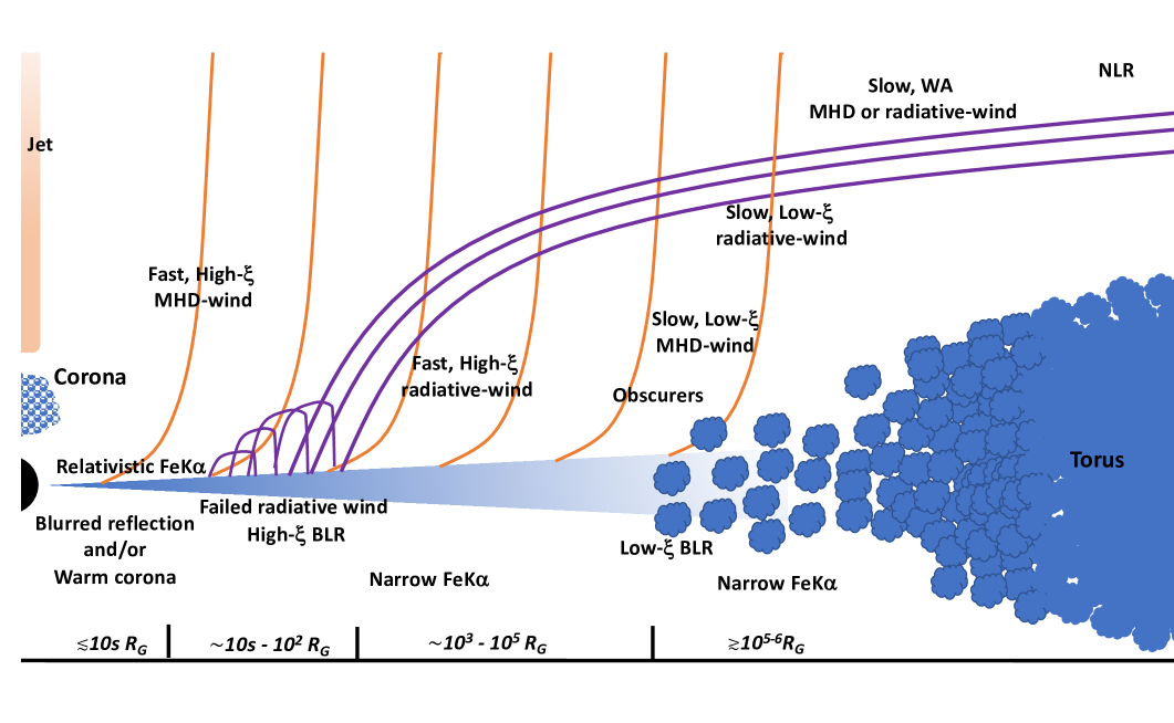
Figure 1: A simple illustration of the AGN region depicting the scales and main components responsible for X-ray emission. The standard accretion disc extends down to the innermost stable circular orbit (ISCO) between $\sim 1.2-6~{}R_{G}$ depending on the black hole spin. The optically thin, hot corona is the primary X-ray source, and it is located close to the SMBH. A collimated jet whose base may coincide with the corona, may or may not be present. The magnetic field lines (orange curves) are the sites of the MHD-driven winds (Section 0.4.2), and they thread the accretion disc over a large range. The streamlines from radiation-driven winds (purple curves; Section 0.4.2) are successfully launched at larger radii where the radiation pressure exceeds the gravitation force in the disc. Within this launching radius, the wind falls back toward the disc, forming a failed wind, which may constitute the inner broad-line region (BLR, Section 0.3.2) and/or shielding gas Proga04 . The disc morphs into the obscuring torus (Section 0.3.2) at large distances, and the traditional warm absorber (WA, Section 0.2) on similar scales. The narrow-line region (NLR) occupies galactic scales, but is photoionised by the AGN. The observer’s line-of-sight will dictate the type of system that is seen and the dominant processes at work. High-resolution spectroscopy will probe the X-ray emission from all these regions.

A simple illustration of the AGN region is depicted in Figure 1. The so-called central engine of the AGN is defined by the accretion disc that funnels material toward the supermassive ($M_{BH}\simeq 10^{6-9}~{}M_{\odot}$) black hole (SMBH). The accretion rate, which is often parameterized by the ratio of the bolometric luminosity over the Eddington luminosity ($\lambda=L_{bol}/L_{Edd}$), will determine the structure of the accretion disc. For moderate values of the Eddington ratio ($\sim 0.01–0.3$), the disc can be approximated as a standard Shakura-Sunyaev disc SS73 that is optically-thick, geometrically-thin, and radiative efficient.

The X-ray emission from the inner-most region within 10’s of gravitational radii ($R_{G}=GM/c^{2}$) is dominated by the hot corona. This primary X-ray source can illuminate the inner disc leading to the production of the reflection spectrum that is blurred by relativistic effects close to the black hole (e.g. RossFabian93 ; Ballantyne01 ; RossFabian05 ). The dominant spectral feature here is the relativistic Fe K$\alpha$ emission line (e.g. Fabian89 ; Laor ). Alternatively, the inner disc region might be blanketed by a warm corona that is optically-thick and conceals the fast inward flow (e.g. wc1 ; wc2 ; Ballantyne20 ).

Winds in the accretion disc are important for transporting angular momentum outward so that material can flow inward (e.g. BH91 ; BP82 ; Murray95 ). Magnetic fields (orange curves in Figure 1) that are capable of launching material out of the system (Section 0.4.2) will thread the accretion disc over large distances. The material in the MHD-driven wind closest to the black hole and moving fastest will also be the most highly ionised since it is closest to the primary X-ray source (i.e. the corona).

Radiative winds (Section 0.4.2) will also be launched from a distance corresponding to where the outward velocity from radiation pressure exceeds the escape velocity in the disc (purple streamlines in Figure 1). At distances closer than the launching radius, the radiation-driven wind will fall back onto the disc. This failed wind region may manifest as many AGN components GP19 ; GP21 and may form part of the highly ionised broad-line region (BLR; Section 0.3.2) in AGN.

On parsec scales, the outer disc morphs into the torus, which is significantly optically thick and neutral. Compton scattering and neutral iron emission are evident here (Section 0.3.2). The traditional warm absorber (WA) will occupy scales similar to these outer disc regions (e.g. Laha14 ; Laha16 ). The WA is responsible for the “normal” velocity winds (Section 0.2) that may be driven by either radiative or MHD effects. The narrow-line region (NLR) occupies galactic scales, but it is still photoionised by the AGN.

There are many intrinsic variations in the AGN phenomenon that likely arise from different accretion rates. However, the observer’s line-of-sight also plays a significant factor Antonucci93 ; Urry95 . The observer’s view through the obscuring torus will determine which disc regions are observable and if the AGN is defined as an unobscured Type I (e.g. Seyfert 1) or obscured Type II (e.g. Seyfert 2). Whether the jet is present, its relative dominance over other AGN components, and the observer’s perspective will dictate if the AGN is radio-loud (jetted) or radio-quiet (non-jetted). The line-of-sight through the winds to the primary X-ray source might also influence the types of winds that are observed.

In the past few decades, tremendous advances were made regarding the X-ray studies of AGN, particularly relating to broadband spectroscopy and variability. The transmission gratings on Chandra (see Chap. 3) and the reflection gratings on XMM-Newton (see Chap. 2) provided glimpses into the discovery space opened by high-resolution spectroscopy. AGN grating data were rich in spectral features, delivering information on gas temperatures, densities, dynamics, and origins. AGN X-ray spectra are not just “power laws”.

As we enter the era of calorimeter spectrometers with XRISM xrism and Athena athena , a new discovery space will be unveiled. With a resolving power $E/\Delta E\approx 1400$, corresponding to $\sim 5$ eV resolution at $\sim 7$ keV, and a collecting area about $10$-times that of Chandra in the Fe K$\alpha$ band, XRISM will transform AGN science in the coming year. We had but a brief, exciting view of this with Hitomi (e.g. hitomi ; perseus ; n1275 ).

In this chapter, we will review and explore the areas of AGN research where high-resolution spectroscopy will make a certain impact. In Section 0.2, the ionised (warm) absorber science that has benefited greatly from grating spectrometers will be reviewed. Later sections focus on the Fe K$\alpha$ band, where calorimeters will resolve these data for the first time. In Section 0.3, the emphasis will be on the nature and origin of the narrow (and broad) Fe K$\alpha$ emission lines. In Section 0.4, the highly-ionised iron seen in absorption and forming ultrafast outflows is examined.

0.2 Warm absorbers

The first detection of absorption from ionised gas in an AGN X-ray spectrum halpern84 opened a new window to study highly ionised nuclear winds. These outflows were subsequently detected and studied by all moderate-resolution CCD cameras: ASCA reynolds97 ; george98 , BeppoSAX (e.g., nicastro00 ; costantini00 ), and ROSAT (e.g., komossa00 ). From these early measurements, the clearest feature in the spectrum was identified as the photoelectric bound-free transition of O vii at $E=0.74$ keV. This feature, detected with different optical depths in most pointed observations of bright AGN, indicated gas with column densities $N_{\rm H}>10^{21}$ cm^-2 george98 . A second feature at $E=0.87$ keV was attributed to the O viii photoelectric edge, suggesting a more ionized component reynolds97 .

A more quantitative characterisation of these WA came with the advent of the high-energy resolution grating spectrometers: XMM-Newton-RGS, Chandra-HETG and Chandra-LETG kaastra00 ; behar01 ; Kaspi01 . Dozens of transitions originating from carbon, nitrogen, oxygen, iron and neon were identified, and the deep absorption edges were no longer the only predictors of ionised absorbers. The feature identified as O vii in earlier studies turned out to be heavily blended with iron transitions from the L-shell to the M-shell, called the iron UTA (unidentified transition array) sako01 ; behar01 . Refinements in the atomic database (e.g., gu01 ; gu06 ) and subsequent studies determined that the iron UTA ions are very sensitive to changes in the ionisation parameter (Figure 2), allowing a robust determination of the state of the gas behar01 ; steenbrugge05 and a diagnostic for gas changes over time (e.g., krongold07 ).

The column density provides a measure of the quantity of gas intrinsic to the source along our line of sight. This does not provide any information on the geometry of the system since neither the thickness nor the density of the gas is directly measurable. The only constraint is that the thickness ($\Delta r$) of the gas cannot be greater than the gas distance from the central source ($r$) blustin05 :

$$\Delta r<r.$$ (3)

A range of column densities spanning more than two orders of magnitude have been reported Laha14 , with the bulk of the gas being in the interval $\rm log({\it N}_{H}/cm^{-2})\sim 20-22$.

In this paper, the ionisation state of the gas is parameterised by tarter69 :

$$\xi=L_{\rm ion}/nr^{2}\hskip 28.45274pt\rm{[erg\,cm\,s^{-1}]},$$ (4)

where $\xi$ is the ionisation parameter, $L_{\rm ion}$ is the ionizing luminosity in the 1–1000 Ryd interval, and $n$ is the gas density. For different values of $\xi$, distinctive groups of ions will be present in the X-ray spectrum. In Figure 2 (left panel), we show the distribution of ionic column densities for the iron ions as a function of log $\xi$. From the spectral point of view, this results in Fe absorption features, among others, distributed all over the X-ray spectrum. In Figure 2 (right panel), we show how iron significantly characterises the absorbed spectrum. For instance, at log $\xi\sim 0.8$, the lower ionisation ions (marked by the iron UTA transitions) are more visible. As log $\xi$ increases, higher ionisation ions are present, originating from other iron L- and K-shell transitions.

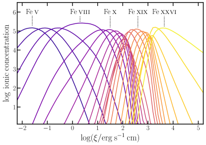
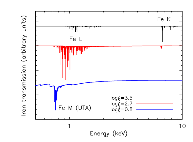
Figure 2: Left panel: The distribution in the concentration of iron ions as a function of log$\xi$. As the ionisation parameters increases, the ion concentration of more ionised Fe is enhanced (courtesy of D. Rogantini). Right panel: The iron transmission spectra for selected values of log$\xi$ highlighting the Fe-UTA, L- and K-shell transitions.

The spectral energy distribution (SED) ranging from the ionisation threshold energy of hydrogen (1 Ryd=13.6 eV) to the end of the canonical X-ray band (1000  Ryd) has a profound impact on the characteristics of the WA. The effects of the UV and soft X-ray spectral shape, as well as the high energy tail of the distribution, have been extensively studied (e.g. nicastro99a ; susmita09 ; susmita12 ). Alongside the distribution of the ionising photons as a function of energy, the metallicity of the WA itself also has a significant influence (e.g. komossa01 ; susmita09 ).

A useful visualisation of these influencing factors is given by the so-called stability curve. This describes, in a log$\xi/T$ vs log$T$ plane, where a WA can exist in equilibrium, for a given SED and metallicity set. The term $\xi/T$ is proportional to the ionisation pressure parameter, $\Xi$, which is the ratio of the radiation pressure over the gas thermal pressure (e.g. rozanska08 ):

$$\Xi\equiv\frac{P_{\rm rad}}{P_{\rm th}}=\frac{L}{4\pi r^{2}c}\frac{1}{nk_{B}T}\propto\frac{\xi}{T}.$$ (5)

Here, $k_{B}$ is the Boltzmann constant and Eq.4 is used to simplify the final formulation. Following susmita09 ; susmita12 , Figure 3 illustrates the behaviour of the thermal stability curve (right panel) as a function of a few key parameters of the SED (left panel).

 

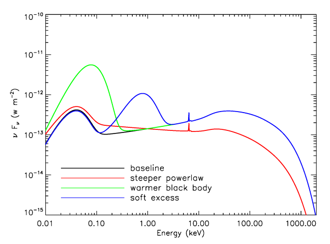
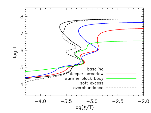
Figure 3: Left panel: Examples of SEDs illuminating the ionized gas (following susmita09 ; susmita12 ). Here, the baseline SED is produced by black body radiation with a temperature 0.01 keV, and a Comptonised component acting at soft X-ray energies with a seed temperature commensurate with the disc. The medium energy is characterized by a power law with a photon index $\Gamma=1.8$ and a reflection component, including the iron emission line, which is cutoff at $E=300$ keV (black solid curve). Right panel: The thermal stability curves for the SEDs displayed in the left panel (solid curves). The curves have been shifted along the x axis, to highlight the different SED effects susmita12 . In addition, the effect of a metal overabundance with respect to solar values is displayed with a dashed curve.

The presence of a stable branch in the curve, that is an almost constant pressure zone for a range of temperatures (e.g., krolik81 ), is enhanced as the power law slope is relatively flat ($\Gamma=1.8$ in this example). Under these conditions, more WA components with different ionisations can co-exist in pressure equilibrium krongold05 . However, the power law slopes are often significantly steeper (up to $\Gamma\sim 2.8$ bianchi09 ). In these cases ($\Gamma=2.1$, red solid curve in Figure 3), the pressure equilibrium zone is disrupted.

The effect of a higher temperature seed black body, or of an enhanced soft excess (green and blue solid curve, respectively in Figure 3), impact the curve at lower values of $\xi/T$, where warm absorbers exist at higher temperatures than in the baseline case, due to heating by iron ions susmita12 .

Element abundances in the WA also have an impact on the stability curve. To emphasize this effect, in Figure 3 (right panel) an overabundance by a factor of five with respect to solar values is displayed (dashed line). The effect is to create a larger zone of pressure stability.

The shape of the SED also influences the type of ions that appear in the X-ray absorption spectrum nicastro99a . A SED typical of a Seyfert 1 galaxy shows a number of absorption lines and photoelectric edges from C, N, and O. Instead, a steeper energy spectrum, for example, characteristic of narrow-line Seyfert 1 (e.g. boller96 ; brandt97 ; Gallo18 ), stimulates iron transitions at different ionisation stages, producing the typical UTA and L- transition arrays at soft energies nicastro99a . For higher ionisation parameters, narrow-line Seyfert 1s display more pronounced iron absorption in the 6–7 keV range (e.g. gallo06 ).

The spectra obtained in the X-rays with high-energy-resolution clearly show that absorption lines displayed a significant blueshift in velocity with respect to the redshift of the AGN host kaastra00 ; Kaspi01 . The blueshift corresponds to WA with velocities in the range $10^{2-3}$ km s^-1 (e.g. Laha14 ). This parameter added the important information that other than an absorbing gas along the line of sight, these components were ejected from the nuclear region towards the host environment. In the same object, different WA components do not necessarily share the same outflow velocity. The distribution of outflow velocities for WA was found to be weakly correlated with the ionisation parameter Laha14 .

Some high-quality spectra of Seyfert 1 galaxies are known to host multiple WA components (e.g. Detmers11 ; kaastra14 ), that differ in ionisation, column density, and outflow velocity. How these components are organized in the AGN system is one of the open questions in this field. As seen above, WA components are only sometimes found to be in pressure equilibrium, where a diffuse, more ionized absorber contains a colder, possibly clumpy, component. Pressure equilibrium would ensure a long-lived gas outflowing structure. In the same object, some WA components are found in equilibrium with each other, in the constant pressure branch of the curve, while others sit in the low ionisation branch (e.g. Detmers11 ).

An intuitive picture (Figure 1) sees the outflows along our line of sight as part of a continuous stream, with the more ionized components located closer to the ionising source (Eq 4). Using Eq. 3 as an upper limit for the radius and assuming that the outflow velocity $v_{out}$ is larger than or equal to the gas escape velocity, a rough range for the location of the absorbers can be found, using this simple geometry blustin05 ; Laha16 . The lower limit on the radius is then given by $r>2GM_{BH}/v^{2}_{out}$. With these estimates, the WA location encompasses a radius range of more than two orders of magnitude, with lower ionisation components located further away Laha16 . Their location seems to be roughly between the broad line region and the molecular torus blustin05 .

The WA components are generally modelled as discrete components, with well-defined parameters. The absorption measure distribution (AMD, holczer07 ; Behar09 ; keshet22 ), describes instead the absorption spectra in terms of a continuous distribution of column densities per unit of log$\xi$ (${\rm d}N_{\rm H}/{\rm d}({\rm log}\xi)$) as a function of log$\xi$. The integral over log$\xi$ would result in the total column density of the WA components. A linear fit of the AMD distribution may be only a simple parameterization, but provides a slope $a$ that may be used as a diagnostic to be compared with theoretical models (see below and Behar09 ). The value of $a$ has been reported to range between $0-0.4$ Behar09 .

Absorption by ionized gas has been mostly associated with radio-quiet objects. The sparse detection in radio-loud, non-blazar objects (e.g. reeves09 ; torresi12 ; digesu16 ), suggests that radio loudness could somehow interfere with the detection of WA, for example, if the object was observed at an unfavourable angle. The X-ray radiation of radio-loud objects being more intense (gupta18 and references therein), was thought to fully ionise the surrounding medium. A systematic study of radio-loud objects in X-rays showed a robust anti-correlation between the power of the radio emission and the column density of the warm absorbers mehdipour19 , independent of the inclination angle and X-ray luminosity. This anti-correlation pointed to a bi-modality between the radio activity and the disk ultimately originating the WA, providing further clues on the origin of the winds.

0.2.1 Obscurers

A category of ionized gas that has been relatively overlooked due to their unpredictable occurrence, has been the so-called “obscurers” (e.g., longinotti13 ; kaastra14 ; mehdipour17 ; kara21 ). This obscuring gas can be formed by one or more high column density ($N_{\rm H}\sim 10^{22-23}$ cm^-2) gas mass, that temporarily obliterates the X-ray soft energy spectrum. This phenomenon became well known from long-term RXTE and Swift light curves, as seemingly normal Seyfert 1 sources, would undergo periods of very hard spectra (high hardness ratios), due to the suppression of the soft X-rays markowitz14 . These sources were sometimes caught in this state, for example by XMM-Newton-pn (e.g. NGC 3516 turner11 , Mrk766 risaliti11 , 1H0419-577 digesu14a ), but without any UV spectroscopic coverage. The limited energy coverage raises different interpretations on whether the hardness ratio is due to absorption or to intrinsic changes in the source (e.g. jiang19 ).

The fortuitous simultaneous observations of NGC 5548 in this spectral state with XMM-Newton, HST-COS, NuSTAR and Integral kaastra14 , allowed for the first time a comprehensive study of this phenomenon. The HST-COS spectrum showed, for every major transition (from C ii up to C iv, N v, and Ly $\alpha$ kaastra14 ), the presence of deep outflows, with velocities in the range 1000–5000 km s^-1. The ionisation parameter of this high-column density gas component is relatively low with log$\xi\sim-(2-1)$, possibly pointing at a dense gas mass. This mass is also not completely covering our line-of-sight ($C_{V}\sim 0.5-1$), changing in both covering factor and column density on a time scale of days–months digesu15 , hinting at a patchy nature for the obscurer.

The degree of absorption correlated with obscuration in the soft X-rays, unequivocally linked the two absorbing agents as the same gas. The location of the obscurer has been estimated to be between the UV-emitting broad line region and the WA. The obscuring gas indeed absorbs the blue side of the broad emission lines in the UV (see Fig. 1 in kaastra14 ). At the same time, the WA components have been found to be photoionised by the central source SED, but significantly modified in shape by the obscurer. This meant that the WA components must have been located at larger distances with respect to the obscuring gas. Instabilities and eruptions in the accretion disks have been invoked to explain the occasional rise of this high-column density gas. However, it is still uncertain why some obscuration events last for almost 10 years (e.g., NGC 5548 mehdipour22 ) and others, occurring in objects of seemingly similar evolutionary state, last only weeks (e.g., NGC 3783 mehdipour17 ). The decline of these disk-wind obscurers is not directly connected to the SED changes, nor to the frequency of their appearance kaastra18 ; mehdipour22 .

Dedicated campaigns, covering the UV and the X-ray band, revealed that many Seyfert 1 galaxies may undergo periods of obscuration during their active life. The study of obscurers also brought to light a complex interplay between the illumination and the covering factors of the UV and X-ray obscurer mao22 ; dehghanian19 ; mehdipour22 . The presence of the obscurer may also describe the X-ray shielding invoked to explain the survival of UV absorbers Proga04 ; dehghanian19 . In addition to the cold patchy components, the occurrence of obscurers has also been associated with an additional component of very high-ionisation gas, with velocity consistent with the cold component, indicating inhomogeneity in the medium, where lower density hems become more ionised mehdipour17 .

0.2.2 The importance of WA and the density determination

As seen above, WA and outflows in general are promising conveyors of feedback into the host galaxy, with important implications for galaxy evolution and formation. In any model predicting the launching mechanism and the impact of outflows on the surrounding medium, it is fundamental to know at what distance the outflow is launched. The rough estimates reported above indicate a range of distances that span orders of magnitudes. This uncertainty is then reflected in Eq. 2. On the other hand, the distance $r$ in Eq. 4 can be calculated from observable parameters only if the density $n$ is known.

A method that has been successfully used in the UV band is density evaluation through density-sensitive absorption lines. These absorption lines are the result of the electron population of a so-called metastable level, above the ground level. The population of this unstable level may be due to both an excess of optical photons in the SED or to the gas with a density above a given threshold, which is different depending on the ion. The column density of the metastable level line is compared to the ground transition and to theoretical curves to find the best fit for the gas density (e.g. korista08 ). Metastable levels of C iii, N iii have been regularly used (e.g. gabel03 ) as well as a number of other UV (Si ii, S iii, P iii, Fe iii arav15 ), and optical transitions (e.g. Fe ii arav08 ). Sometimes, the metastable line happens to be part of a WA component that is visible both in the UV and the X-rays, providing a density estimate also for the X-ray absorber costantini10 ; edmonds11 ; digesu13 . In the X-ray band, only one detection of O v has been reported for an AGN so far kaastra04 , leading to a lower limit for the gas density.

Methods that may be easier to apply, make use of the response of the gas as a function of the ionizing luminosity (Eq. 4). Every ion in a gas will have its own reaction time, depending on the density of the gas krolik_kriss95 ; nicastro99b ; rogantini22 . In particular, the time taken for the gas to react is inversely proportional to the gas density. The time dependence of the ionic concentration of a certain element $X$, $n_{\mathrm{X}^{i}}$ can be written as:

$$\frac{dn_{\mathrm{X}^{i}}}{dt}=-n_{\mathrm{e}}n_{\mathrm{X}^{i}}\alpha_{\mathrm{rec},\mathrm{X}^{i-1}}-n_{\mathrm{X}^{i}}I_{\mathrm{X}^{i}}+n_{\mathrm{e}}n_{\mathrm{X}^{i+1}}\alpha_{\mathrm{rec,X}^{i}}+n_{\mathrm{X}^{i-1}}I_{\mathrm{X}^{i-1}}.$$ (6)

Here, $n_{\mathrm{e}}$ is the electron density, while $I_{\mathrm{X}^{i}}$ and $\alpha_{\mathrm{rec,X}^{i}}$ are the ionisation and recombination rates between state $i$ and $i+1$.

In Fig. 4, the behaviour of Fe xx as a function of time is illustrated for a range of gas densities. The higher the column density the more the gas response approaches an instantaneous change as a function of the flux variation, leaving the gas in equilibrium conditions at every time. If, on the contrary, the gas density is very low, the signal is diluted and no variation in the gas is observed. For a range of densities (log($N_{\rm H}/{\rm cm}^{-2})\sim 5-7$), Fe xx reaction time is significantly delayed.

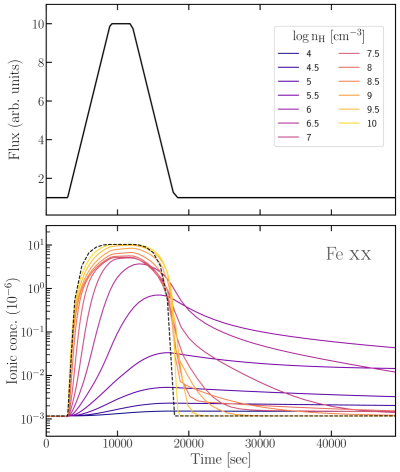
Figure 4: Upper panel: An example of a flaring light curve. Lower panel: The ionic concentration of Fe xx response to the time evolution of the flux change. The equilibrium condition (i.e. instantaneous response, following Eq. 4) is marked with a dashed line. Depending on the density, the gas will respond with a different delay, as highlighted by the colour-coded solid lines. Adapted from rogantini22 .

In principle, Eq. 6 can be used for every source whose flux significantly changes in time. In practice, this method, that relies on time-resolved spectroscopy, is often limited by the signal-to-noise per time bin of the spectrum. A slow variation may lead to subtle variations in the WA that are difficult to detect kaastra12 , while strong and sudden variations require that the WA is analysed on few-kilosecond time bins, therefore reducing the quality of the spectrum krongold07 . Several estimates of the density, and therefore on the distance, of the WA have been reported. Only a few experiments were successful in putting limits on the distance of the WA. For example, krongold05 derived an upper limit of $r<6$ pc for a gas component in NGC 3783, consistent with the limit ($r<25$ pc) derived for the same gas component from the analysis of the UV data gabel05 .

In Mrk 509, the general lack of variability in the WA set the lower limits to relatively far distances for the different components (ranging from about 5 pc up to 70 pc, with some components at kpc scales kaastra12 ). A similar range, spanning from parsecs to tens of parsecs, has been found for the WA components of NGC 985 ebrero21 . Smaller black hole systems, like in the narrow-line Seyfert 1 galaxies, show instead the desired large variation in flux on time scales of few kiloseconds. An intensively studied object of this class is NGC 4051, where the WA components were found to be closer to the black hole, around 1 light day distance (e.g., krongold07 ; steenbrugge09 ).

0.2.3 Future outlook on warm absorbers

The design of future high-resolution instruments would certainly reward the study of ionised absorbers. High-sensitivity, high-resolution ($\Delta E\leq 5$ eV) calorimeters (XRISM, xrism and Athena-XIFU athena ) will bring significant advancement, for example, in the study of variable WA and the determination of the gas density. In the future, time-resolved spectra will allow us to follow the evolution of multi-components in WA as a function of time rogantini22 . At the same time, different applications of Eq. 6 will be possible, for instance combining timing and spectroscopy silva16 . The coherence between two signals, in this case between the continuum and the warm absorber, as a function of energy, bears the signature of the time delay of the recombining gas and therefore of the gas density juranova22 . This can be detected and studied provided high-sensitivity and resolution data (Figure 5).

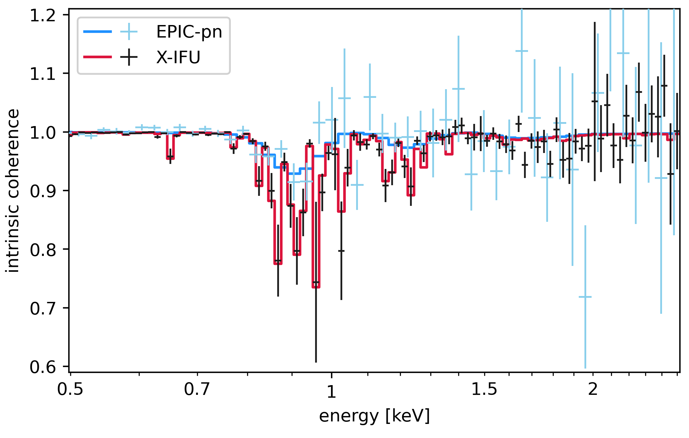
Figure 5: Athena-XIFU simulation (red data points and solid line) of the coherence as a function of energy for a typical narrow-line Seyfert 1 source hosting a WA. This is compared to the capabilities of current high-sensitivity instruments (e.g., XMM-Newton EPIC-pn, blue data points and solid line). The shape of the coherence spectrum as a function of frequency can be modelled to solve for the gas density. Modified from juranova22 .

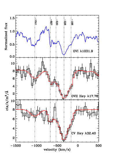
Figure 6: Arcus simulation of the non-saturated $\gamma$ lines of the He-like series for O vii and C v, respectively (middle and lower panels), compared to the HST-STIS velocity resolved profile of one of the doublet components of O vi ($\lambda 1031.9\AA$) (upper panel crenshaw03 ).

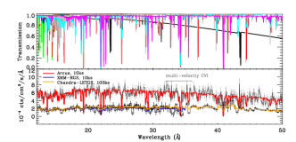
Figure 7: A 10 ks simulation using a next generation soft-X-ray grating ($\lambda/\Delta\lambda>2500$). The simulation includes a six-component WA kaastra14 and Galactic cold absorption (upper panel). The grating simulation is compared with XMM-Newton-RGS and Chandra-LETGS (lower panel). The data have been rebinned and shifted along the vertical axis for clarity.

New generation grating spectra (as in the mission concept Arcus smith16 ), operating in the soft-X-ray energy, will permit studying the kinematics of the absorbers (Figure 6) and line absorption profiles, as routinely performed in the UV band. The envisaged resolution ($\lambda/\Delta\lambda>2500$) and a large effective area compared to XMM-Newton-RGS, will allow us to perform different density diagnostic tests, including the detection of metastable levels mao17 and time-resolved spectroscopy rogantini22 on a large number of sources (Figure 7).

0.3 Fe K emission lines in AGN

0.3.1 The atomic physics of Fe K emission lines

Narrow emission lines from the Fe K shell are the most prominent atomic feature in the X-ray spectra of AGN. Typically, a single emission line is seen in addition to a local continuum that can be approximated with a power law. These lines are produced when ionizing X-ray radiation illuminates relatively cold, dense gas. In this sense, narrow Fe K lines trace the interaction of the central engine with the accretion flow on all scales, and can serve to test models for its (sub-)structure and evolution. Indeed, hard X-ray emission from the central engine can even excite narrow Fe K lines on scales that are better associated with the larger host galaxy than the accretion flow. The “X-ray reflection nebulae” in the center of the Milky Way, for instance, likely indicate that Sgr A* was much more luminous $few\times 10^{4}$ years ago Koyama96 (also see Ponti15 ).

It is important to clarify that Fe K-shell lines are only prominent within the spectra of AGN owing to a combination of three key factors: (1) a relatively high fluorescence yield, (2) a relatively high abundance, and (3) the Fe K lines fall within a part of the spectrum that is otherwise relatively simple. The fluorescence yield of an atomic shell is simply the probability that a vacancy results in a radiative transition, rather than the ejection of an Auger electron. The K-shell fluorescence yield is positively correlated with atomic number Bambynek72 . By a factor of $\sim 5$, Fe is the element with the highest product of fluorescence yield and abundance GF91 . Fluorescence lines from the K-shell of more abundant elements with lower yields are also excited when Fe K-shell lines are excited; they are just less prominent.

A narrow Fe K emission line in the spectrum of a given AGN is often referred to as “the neutral Fe K” line or “the neutral Fe K$\alpha$ line.” These colloquial terms are convenient, especially at modest sensitivity and/or modest spectral resolution. However, the situation is more complex, and this may become readily apparent in the era of calorimeter spectroscopy. It is therefore worth undertaking a quick overview of the key atomic physics, before reviewing some key recent developments with Chandra, XMM-Newton, and other telescopes.

The neutral Fe K$\alpha$ fluorescence line arises from a 2p-1s electron transition, and the spin-orbit interaction therefore creates two lines with a small energy difference: K$\alpha_{1}$ at 6.404 keV and K$\alpha_{2}$ and 6.391 keV, with a 2:1 branching ratio Bambynek72 . This difference, just $\Delta E=13$ eV, exceeds the $\Delta E=5$ eV energy resolution that was achieved with the calorimeter aboard Hitomi hitomi ; the “Resolve” calorimeter that will fly aboard XRISM in 2023 is expected to have the same resolution xrism . The X-ray Integral Field Unit (XIFU) spectrometer expected to fly aboard Athena in the 2030s is expected to have a resolution of just $\Delta E=2.5$ eV.

The upper panel of Figure 8 shows a model spectrum constructed using mytorus mytorus owing to its physical self-consistency, and because it has a native resolution of just 2 eV and is therefore suited to even calorimeter spectra mytorus ; Yaqoob12 . It depicts an Fe K emission spectrum from neutral gas, broadly characteristic of the spectra observed in Seyfert 1 AGN. The model was constructed according to the prescriptions in Kammoun20 assuming an obscuring column density of $N_{H}=1\times 10^{22}~{}{\rm cm}^{-2}$ and an inclination of $\theta=30^{\circ}$. At high resolution, the Fe K$\alpha_{1}$ and Fe K$\alpha_{2}$ lines are easily separated, and the corresponding Fe K$\beta$ line is also clearly represented.

The weighted average of these two lines is $E=6.3997\simeq 6.40$ keV, but if the two lines are fit with a single Gaussian – common in non-calorimeter data – it is then important to account for the two lines in any determination of the line production radius based on virial or Keplerian motions. The energy difference between the two corresponds to a broadening of $\Delta E/E\simeq 600~{}{\rm km}~{}{\rm s}^{-1}$ that must be subtracted before estimating the production radius.

Most of the strong Fe K lines that are observed in AGN are statistically consistent with being neutral; however, this does not automatically signal that the emitting gas is neutral. The weighted mean line energy of Fe i is 6.40 keV, but this only changes to 6.43 keV for Ne-like Fe xvii Bautista03 ; Bautista04 ; Palmeri03a ; Palmeri03b ; Mendoza04 (also see NIST ). Even for grating spectrometers and CCD spectrometers, a difference of just $\Delta E=30$ eV is often within the measurement uncertainty in data of modest sensitivity.

As we look ahead to the era of calorimeter spectroscopy, will realistic doubts about the ionisation of the emitting gas be resolved? Potentially, but not necessarily. Consider a line of sight that views the optical broad line region at an inclination of $\theta=45^{\circ}$, potentially appropriate for a Seyfert 1.5 AGN. Our line of sight may reveal more of the face of the BLR that is on the far side of the central engine. If the BLR is an outflow, an Fe K line produced within it may be red-shifted relative to the host frame of reference. A line from Ne-like Fe xvii at 6.43 keV would only have to arise in an outflow with a velocity of $v\simeq 1400~{}{\rm km}~{}{\rm s}^{-1}$ to appear to be consistent with neutral Fe i. The K-shell edge for Fe xvii lies at 7.8 keV, whereas the edge for Fe i lies at 7.1 keV. Emission lines are often much easier to detect than associated edges, but the detection of K-shell edges would nominally distinguish neutral gas with no velocity shift from ionized gas that is shifted to be coincident with other charge states.

It is also important to appreciate that the fluorescence yield changes with ionisation, not just atomic number. Between Fe i and Fe xxii, the fluorescence yield slowly rises from $Y_{\textup{Fe\,{i}}}=0.34$ to $Y_{\textup{Fe\,{xxii}}}=0.49$ Bambynek72 , but falls to $Y_{\textup{Fe\,{xxiii}}}=0.11$ for Fe xxiii, recovering to $Y_{\textup{Fe\,{xxiv}}}=0.75$ for Fe xxiv, and has values of $Y_{\textup{Fe\,{xxv}}}=0.5$ and $Y_{\textup{Fe\,{xxvi}}}=0.7$ for He-like Fe xxv and H-like Fe xxvi (see KK87 , and references therein). This has important consequences for breaking degeneracies between charge state and velocity shifts in data with modest sensitivity. In a given scenario, it may be more likely that an observed line represents blue- or red-shifted emission from a charge state with a high yield, rather than a line from a charge state with a low yield from gas that is largely at rest.

When Fe K lines are produced in optically thick gas (e.g., the accretion disk, the molecular “torus”, or even cold clumps within the optical broad line region or disk winds), they are part of a larger reaction spectrum that is called “X-ray reflection” (e.g. GF91 , and many others). As noted above, this process includes the production of lines from other abundant elements, but there are two other prominent attributes. One is an absorption trough owing to the Fe K-shell photoelectric absorption edges (7.1-9.3 keV, depending on the ion). The other is known as the “Compton hump,” generally peaking between 20-30 keV. This is not a true flux excess; rather, it is the result of the albedo of the cold gas peaking in this range. Higher energy X-rays penetrate deeply into the accretion disk and thermalize. In combination with the photoelectric absorption trough at low energy, the effects combine to yield a “hump” that appears above the power law observed from the central engine.

The preceding discussion has focused on the narrow core of Fe K lines. The narrow core represents the line flux that escapes from the irradiated cold, dense gas without being scattered within the emitting region. Some fraction of the line photons will scatter, though, giving rise to a series of Compton shoulders (e.g., GF91 ; Matt02 ). These shoulders take the form of a plateau that extends redward of the core, abruptly ending in a cliff at 6.24 keV, set by the maximum energy that a photon loses in a $180^{\circ}$ scattering event. Up to the optically thick limit, it is more likely that a photon will scatter once than multiple times, and the first Compton shoulder is the only one that is anticipated in actual data. The relative strength of the Compton shoulder and narrow core is a function of the column density of the emitting region, and the inclination angle. Relative to the narrow core, the first shoulder is more pronounced with increasing column density, peaking in material that is Compton-thick, and at low inclinations, because the scattered photons originate deeper in the slab than the unscattered ones Matt02 .

The lower panel in Figure 8 shows another model spectrum generated using mytorus mytorus . In this case, the obscuring column density was set to be $N_{H}=2\times 10^{24}~{}{\rm cm}^{-2}$, making the emitting gas Compton-thick. The first Compton shoulder is clearly evident from both the Fe K$\alpha$ lines and Fe K$\beta$ lines. In this idealized example, the second K$\alpha$ Compton shoulder is also visible, extending down to 6.1 keV. It is possible that the second shoulder may be detected in the best calorimeter spectra, but it may be more readily detected in an X-ray binary like GX 301-2 Watanabe03 than in an AGN.

Figure 8: Spectral models depicting line production in the Fe K region of AGN spectra, generated using the mytorus code mytorus ; Yaqoob12 , also see Kammoun20 . In the upper panel, the line production region has column density of $N_{H}=1\times 10^{22}~{}{\rm cm}^{-2}$. In the lower panel, the line production region has a column density of $N_{H}=2\times 10^{24}~{}{\rm cm}^{-2}$, making it Compton-thick. These models were constructed assuming neutral gas and a viewing angle of $\theta=30^{\circ}$. In both cases, the two Fe K$\alpha$ lines are apparent, as well as the Fe K$\beta$ line. However, in the Compton-thick case, the first Compton shoulder is visible, owing to $180^{\circ}$ scattering in the gas.

0.3.2 The nature and origin of “narrow” Fe K emission lines in AGN

“Does the narrow Fe K line originate in the torus, or in the optical broad line region?”

This simple question has been at the heart of many investigations using CCD and grating spectrometers over the last two decades. It is built on solid expectations: above a certain threshold in the Eddington fraction, optical “broad line regions” and cold, obscuring torii appear to be ubiquitous in AGN. Since it is the torus that determines whether or not the broad line region is visible in a given source, and since obscured and unobscured AGN are roughly equal in number, it is logical to conclude that torii likely occupy approximately half of the sky as seen from the central engine. A reasonable hypothesis, then, is that the torus overwhelmingly dominates the flux observed in narrow Fe K lines, and the dichotomy underlying this question is justified.

A few considerations argue otherwise and suggest that this is an ill-posed question. First, every geometry that is at least partially composed of cold, dense gas will contribute Fe K line flux when it is irradiated by hard X-rays. Second, the line flux that is contributed by a given geometry depends on the hard X-ray flux received at that radius, not just its solid angle. Finally, but perhaps most importantly, the broad line region and torus may not be as physically distinct as some results would suggest. Although some torii have been imaged in IR bands using interferometric techniques, and clearly span parsec scales, this does not convey the innermost extent of the torus. Dust reverberation mapping in a growing number of quasars finds that the torus is only $\sim$5 times larger than the optical broad line region Minezaki19 . If the presence of dust marks the innermost extent of a cold, dusty, molecular torus, then the torus is simply not much larger than the broad line region, and it may not be productive to treat them as entirely separate (see Figure 1).

The Chandra-High Energy Gratings (HEG) have a nominal resolution of 45 eV at 6.4 keV, in the first-order spectra (see Chap. 3). While this is several times sharper than the resolution afforded by CCD spectrometers, such as the EPIC-pn aboard XMM-Newton, the effective area of the HEG in the Fe K band is $A_{eff}\simeq 30~{}{\rm cm}^{2}$, whereas that of the EPIC-pn is $A_{eff}\simeq 900~{}{\rm cm}^{2}$. Observations with the Chandra-HEG are therefore better suited to measurements of Fe K line widths, and corresponding production radii and widths.

An early, 83 ks Chandra observation of NGC 5548 measured a line centroid energy of $E=6.402^{+0.027}_{-0.025}$ keV, and a width of $FWHM=4515^{+3525}_{-2645}~{}{\rm km}~{}{\rm s}^{-1}$ Yaqoob01 . Even in a moderately deep grating spectrum, Fe xvii (E = 6.43 keV) was not excluded. The error bars on the line width are large in the fractional sense, but point to an origin in the optical BLR rather than in gas that is confined to parsec scales. The uncertainties in these measurements partially reflect the limited effective area of the HEG.

Chandra made a much longer, 900 ks observation of NGC 3783. The Fe K line centroid was measured to be $E=6.3982~{}{\rm keV}\pm 3.3$ eV, and the line width was measured to be $FWHM=1720\pm 360~{}{\rm km}~{}{\rm s}^{-1}$ Kaspi01 . The line width is again consistent with the outer broad line region and/or the innermost extent of a small torus, rather than gas at the scale of a parsec. This effort also detected the first Compton shoulder in the Fe K line profile, indicating an origin in optically-thick material.

Additional Chandra-HEG spectra of Seyfert-1 made it possible to compare the width of Fe K$\alpha$ emission lines to optical H$\beta$ lines from the BLR. An early systematic comparison examined literature values in 14 sources, and found that (1) the average Fe K$\alpha$ line width is a factor of $\sim 2$ lower than the corresponding H$\beta$ line, and (2) that there is no correlation between the line widths Nandra06 . The key conclusion of this analysis was that the narrow Fe K$\alpha$ line originates in the torus. Many intervening years and results make it possible to see this conclusion in context. At the time, the torus was typically envisioned as a parsec-scale geometry; the FWHM differences do not necessitate that; rather, the contrast is broadly consistent with much smaller contrast indicated by dust reverberation mapping Minezaki19 .

A more detailed examination of the growing number of sensitive Chandra spectra of Seyfert 1 AGN, and a comparison to H$\beta$ lines in each source, was reported in 2010 Shu10 . A total of 82 Chandra observations from 36 sources were considered, explicitly allowing for variations in the line properties between observations. In a subsample of 27 source, the mean Fe K$\alpha$ line width is measured to be $\langle FWHM\rangle=2060\pm 230~{}{\rm km}~{}{\rm s^{-1}}$, and no correlation is found between Fe K$\alpha$ and H$\beta$ line widths. The more detailed nature of this survey permitted a more nuanced and very important finding: “There is no universal location of the Fe K$\alpha$ line-emitting region relative to the optical broad line region (BLR). In general, a given source may have contributions to the Fe K$\alpha$ line flux from parsec-scale distances from the putative black hole, down to matter a factor of $\sim$2 closer to the black hole than the BLR” Shu10 .

Andonie et al. Andonie22 have undertaken the most recent and expansive examination of narrow Fe K$\alpha$ emission line regions. Their analysis included 38 bright AGN in the Neil Gehrels Swift Observatory Burst Alert Telescope (BAT) Spectroscopic Survey. Utilizing Chandra images and spectra, XMM-Newton spectra, and variability studies, independent estimates of the Fe K$\alpha$ production radius ($R_{Fe~{}K}$) were obtained and compared to plausible estimates of the dust sublimation radius ($R_{subl.}$) in each source. In the cases where data permitted measurements of the line FWHM, the $R_{Fe~{}K}<R_{subl.}$ in 90% of the sources (21/24 AGN). Similarly, in the cases where significant line variability was detected, $R_{Fe~{}K}<R_{subl.}$ in 83% of the sources. Andonie et al. Andonie22 conclude that Fe K$\alpha$ lines in unobscured AGN typically originate in the outer part of the BLR, or the outer disk, but carefully note that “the large diversity of continuum and narrow Fe K$\alpha$ variability properties are not easily accommodated by a universal scenario.”

The left hand panel in Figure 9 shows the Fe K$\alpha$ emission radius versus an estimate of the dust sublimation radius. The Fe K$\alpha$ emission radius was calculated based on the velocity width of the line, and the dust sublimation radius was estimated using an expression derived by Nenkova08 , and assuming that graphite sublimates at $T=1500$ K. The figure illustrates that the Fe K$\alpha$ line production radius is systematically smaller than the dust sublimation radius within the sample. If we take the dust sublimation radius as indicative of the innermost extent of the torus, this finding is at least qualitatively consistent with the dust reverberation results of Minezaki19 . The right hand panel in Figure 9 depicts the Fe K$\alpha$ emission line radius versus the H$\beta$ production radius. There is no clear trend within the data; only a few AGN clearly lie above or below the line that marks an equivalent production radius, and many Fe K$\alpha$ line production radii carry relatively large uncertainties.

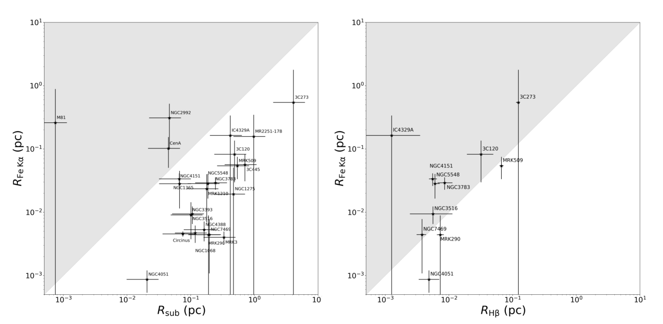
Figure 9: These panels summarize some of the key results obtained in the survey of Seyfert Fe K$\alpha$ lines undertaken by Andonie22 . At left, the Fe K$\alpha$ line production radius (measured via line widths) is compared to an estimate of the dust sublimation radius – a proxy for the innermost extent of the dusty torus – in each AGN. The Fe K$\alpha$ line production regions are found to occur at smaller radii, strongly suggesting that the bulk of the emission seen in unobscured AGN is produced within the BLR or in even more compact regions. At right, the Fe K$\alpha$ line production radius in each AGN is compared to the H$\beta$ production radius, the characteristic radius of the optical BLR. The data do not appear to permit a systematic statement, but it is fair to conclude that the production radii are broadly comparable. (This figure is reproduced from Andonie22 , with permission.)

Figure 10 shows a comparison of summed Chandra-HEG spectra from the Seyfert 1 NGC 4151 in its high and low flux states, and the summed HEG spectrum of the Compton-thick Seyfert 2 NGC 1068. The opposing first-order spectra were added, the spectra have been shifted in energy to their respective rest frames, and the flux of NGC 4151 has been adjusted to the distance of NGC 1068. No spectral fits were made. Recent estimates suggest that the mass of the black hole in NGC 1068 is $M=1.5\times 10^{7}~{}M_{\odot}$ Morishima22 ; optical reverberation mapping gives a formally equivalent black hole mass in NGC 4151: $M=1.66^{+0.48}_{-0.34}\times 10^{7}~{}M_{\odot}$ Bentz22 . For these mass estimates, NGC 1068 is likely accreting at an Eddington fraction at or below $\lambda\leq 0.2$ Bland97 , and NGC 4151 at a rate of $\lambda=0.03-0.04$ Miller18 . Given their similar masses, the fact that NGC 1068 is likely surrounded by gas with a higher filling factor and likely accreting at a higher rate than NGC 4151, it should show a stronger neutral Fe K$\alpha$ emission line in this comparison. However, the opposite is the case. This can be explained if the gas that is emitting the Fe K$\alpha$ line within our line of sight in NGC 4151 is closer to the central engine than the emitting gas within our line of sight is in NGC 1068. Without any spectral modeling, this example illustrates that different views of the central engine actually reveal different regions, and that faulty conclusions may be drawn if a single emitting geometry is invoked.

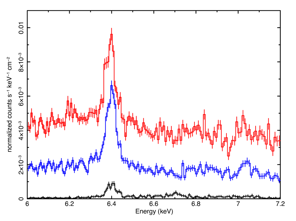
Figure 10: A comparison of spectra from the Compton-thick Seyfert 2 AGN NGC 1068 (black), and NGC 4151 in its high (red) and low (blue) flux states. The spectra are the summed Chandra-HEG spectra from each source, shifted to their host frame. The flux of the NGC 4151 spectra have been shifted to the smaller distance to NGC 1068. The inferred black hole masses and Eddington fractions in these AGN are broadly similar (see the text for details), enabling a consistent comparison. If the covering factor of cold, dense gas were the only factor that determined line strength, the narrow Fe K$\alpha$ line in NGC 1068 should be much stronger. However, factors including the distance of the gas to the responding medium also matter, and this is likely the reason that the line is stronger in NGC 4151. This figure illustrates that different viewing angles and obscuration properties can reveal different regions, not necessarily different aspects of the same emission region.

0.3.3 The approaching calorimeter era

A number of recent results highlight the potential of X-ray calorimeter spectroscopy to reveal the inner accretion flow onto massive black holes. Here, we highlight four key results that likely provide an early glimpse of the science that will be enabled by the sharper resolutions and larger effective areas afforded by XRISM and Athena.

In a major departure from phenomenological Gaussian modeling, and simple comparisons of Fe K$\alpha$ and H$\beta$ line widths, Costantini10 examined the spectrum of the Seyfert 1 Mrk 279 using the Local Optimally emitting Cloud model (LOC; Baldwin95 ). This model does not assume a geometry for the BLR; rather, it simply assumes that each line is the result of contributions from multiple regions that follow a power law distribution in gas density and radius. Mrk 279 is particularly interesting among Seyferts, in that its “narrow” Fe K$\alpha$ line appears to be composed of an unresolved core and a $FWHM=14,000~{}{\rm km}~{}{\rm s}^{-1}$ component.

By first establishing the parameters of a LOC model using UV and soft X-ray lines and then extending the model to the Fe K band, costantini07 ; Costantini10 show that the BLR model can account for only 3-17% of the Fe K$\alpha$ broad line flux. A subsequent study using the same technique, based on simultaneous optical, UV, and X-ray observations of Mrk 509, costantini16 established that the contribution of the BLR to the Fe K$\alpha$ line could be up to 30%. The clear implication is that part of the Fe K$\alpha$ line in these two objects originates at smaller radii than the optical, UV, and even soft X-ray BLR, while the unresolved line core may be produced in the torus at larger radii. If these cases are not unique, but rather just an AGN that offers a fortuitous view of its inner disk, BLR, and torus, moderately deep observations of Seyfert-1 AGN with XRISM may readily decompose seemingly monolithic lines into such components.

NGC 4151 is the brightest Seyfert AGN in the 4-10 keV band, with the strongest narrow Fe K$\alpha$ line observed in any Seyfert 1 (e.g., Shu10 ). As such, it can be expected to deliver the most sensitive spectra and important hints of the potential of calorimeter spectroscopy with XRISM and Athena. These expectations led Miller18 to examine Chandra-HEG spectra of NGC 4151. The total summed spectrum (631 ks of exposure), and spectra summed from low (337 ks) and high (294 ks) flux states were examined. In each case, the line profile is found to be asymmetric and red-skewed, suggestive of weak relativistic Doppler shifts (see Figure 11). Fits with a number of independent models imply line production radii in the $R=500-1000~{}GM/c^{2}$ range. This again implies that the bulk of the “narrow” Fe K line flux originates at smaller radii than the optical BLR.

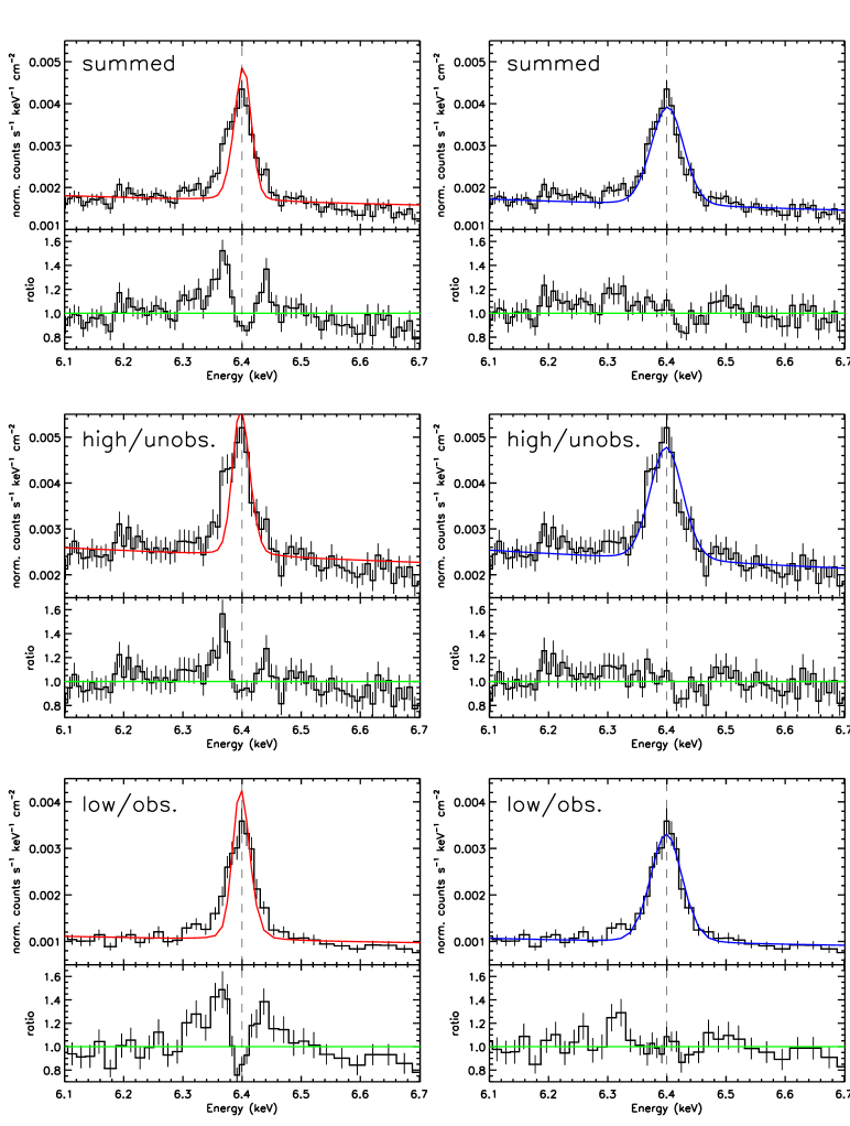
Figure 11: Fits to the “narrow” Fe K$\alpha$ line in summed Chandra-HEG spectra of NGC 4151 Miller18 . The spectra were shifted to the rest frame and binned for sensitivity and visual clarity. The left hand panels depict the results of fits with Gaussian profiles that only have instrumental broadening; while the right hand panels depict fits with Gaussian profiles with a variable width. The line is clearly asymmetrical, with excess flux to the red; a variety of models that include weak relativistic Doppler shifts and gravitational red-shifts suggest an inner production region of $R=500-1000~{}GM/c^{2}$, considerably smaller than the optical BLR. (This figure is reproduced from Miller18 , with permission).

NGC 4151 may also provide early hints that the region between the innermost disk and optical BLR is structured. Miller et al. Miller18 find that the high-low flux difference spectrum reveals a line profile with two peaks, red-shifted from the expected narrow line core and Compton shoulder; fits to this profile require a narrow ring of emission between $R=70-120~{}GM/c^{2}$ (see Figure 12). Independently, within the spectra typified by a high continuum flux, the Fe K$\alpha$ line flux appears to vary on time scales of $\Delta t\simeq 2\times 10^{4}~{}{\rm s}$, implying $R\simeq 50-130~{}GM/c^{2}$. These findings are at least qualitatively consistent with a warp or ring-like structure, similar to the features seen in numerical simulation of accretion flows when the angular momenta of the black hole and accretion flow are misaligned (e.g., Nixon12 ).

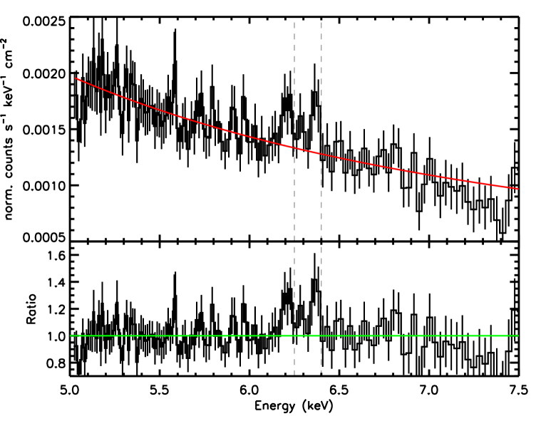
Figure 12: The difference spectrum obtained when the summed Chandra-HEG exposure in the low flux state is subtracted from the summed exposure in the high flux state Miller18 . The spectrum was shifted to its rest frame, binned, and fit with a simple power-law. The lingering Fe K$\alpha$ emission is red-shifted from the expected value of $E=6.40$ keV, and equally strong emission is red-shifted from the Compton shoulder at $E=6.25$ keV, though the narrow core and shoulder are not expected to be comparably strong. The residual structure is suggestive of a warp or a ring in the inner disk extending between $R=50-130~{}GM/c^{2}$, potentially enhanced with a higher mass accretion rate and/or stronger irradiation. (This figure is reproduced from Miller18 , with permission).

Zoghbi et al. Zoghbi19 reported the first detection of reverberation in the narrow Fe K$\alpha$ line in any AGN. Again owing to its flux, this detection was made in NGC 4151, using data from XMM-Newton and Suzaku. The flux sensitivity of these data outweighed their modest resolution relative to the Chandra-HEG. Using the javelin code that is widely implemented to measure lags from the optical BLR Zu13 , Zoghbi et al. Zoghbi19 measure a delay of $\tau=3.3^{+1.8}_{-0.7}$ days (see Figure 13). For plausible black hole masses, this light travel time is broadly consistent with the radii measured via fits to the Fe K$\alpha$ line shape observed with Chandra Miller18 .

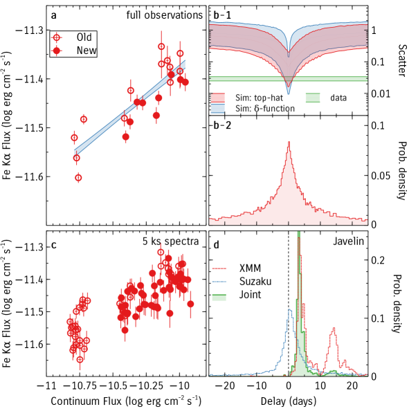
Figure 13: Evidence of a reverberation lag in the narrow Fe K$\alpha$ line in NGC 4151 Zoghbi19 , based on numerous observations with XMM-Newton and Suzaku. Panel (a) shows a strong correlation between the Fe K$\alpha$ flux and continuum flux measured across full exposures. Panel (b1) shows the scatter in the line–continuum relation in different simulations that sample different delay times. Panel (b2) shows the probability density of the different delay times. Panel (c) shows the line–continuum relation, taking 5 ks segments instead of full observations. Finally, panel (d) shows the probability density for different values of the lag using the 5 ks segments. A lag of $\tau=3.3^{+1.8}_{-0.7}$ days is measured, yielding a black hole mass of $M=1.8^{+2.2}_{-1.1}\times 10^{7}~{}M_{\odot}$ assuming the line widths measured by Miller18 . This is fully consistent with the most recent optical reverberation mass, $M_{BH}=1.66^{+0.48}_{-0.34}\times 10^{7}~{}{\rm M}_{\odot}$ Bentz22 .

Using the standard equation to derive the black hole mass, $M_{BH}=fc\tau v^{2}/G$ (where $f$ is a geometric factor derived via comparisons to direct primary masses, and $v$ is the width of the line), Zoghbi19 infer a mass of $M_{BH}=1.8^{+2.2}_{-1.1}\times 10^{7}~{}M_{\odot}$, assuming a standard value for the geometric factor ($f=4.13\pm 1.05$; Grier13 ) and the line width measured using Chandra. This value agrees extremely well with the most recent optical reverberation mass, $M_{BH}=1.66^{+0.48}_{-0.34}\times 10^{7}~{}{\rm M}_{\odot}$ Bentz22 . Future studies may find that the geometric factor is not the same for the X-ray and optical gas, and/or that the responding geometries vary with time. However, this initial detection and plausible mass estimate suggest a bright future for narrow Fe K$\alpha$ reverberation studies.

Another detection of reverberation in a narrow Fe K$\alpha$ line was recently reported in archival Suzaku observations of the bright Seyfert 1 AGN NGC 3516 Noda22 . Again using javelin Zu13 , a lag of $\tau=10.1^{+5.8}_{-5.6}$ days is measured. Importantly, the lag is only found during a period when NGC 3516 was particularly faint in X-rays, and similar to a Seyfert 2 AGN. In those cases, the BLR is typically blocked by the torus, so the fact that reverberation mapping was still possible using the Fe K$\alpha$ line may signal that XRISM and Athena can measure lags and black hole masses in cases where optical attempts have not been successful.

XRISM spectra will likely achieve a resolution of $5$ eV and an effective area close to $A_{eff}\simeq 300~{}{\rm cm}^{2}$ in the Fe K band. Both represent order-of-magnitude improvements over the capabilities of the Chandra-HEG. Although this effective area does not exceed that of the EPIC-pn CCD camera aboard XMM-Newton, its superior resolving power will make XRISM far more sensitive to lines. It is therefore worth asking: in how many AGN will XRISM achieve similar and better results, assuming optimal conditions (e.g., a 10-year mission with consistent instrumental performance)?

XRISM will be revolutionary, but it is still a small telescope (in some sense, a pathfinder for Athena). The extraordinary time required to achieve sensitive spectra of faint AGN would necessarily come at the expense of fully understanding the demographics of a brighter sample. For such reasons, it is pragmatic to set a flux limit. In general, only Seyferts with a flux above $F\simeq 1\times 10^{-11}~{}{\rm erg}~{}{\rm cm}^{-2}~{}{\rm s}^{-1}$ in the Chandra pass band have enabled significant line detections in exposures of $1-9\times 10^{5}~{}{\rm s}$. A broad view of surveys undertaken with ROSAT, XMM-Newton, and eROSITA suggests that there are roughly 300 AGN with an X-ray flux of $F\geq 1\times 10^{-11}~{}{\rm erg}~{}{\rm cm}^{-2}~{}{\rm s}^{-1}$ in the 0.5-10 keV band Voges99 ; Saxton08 ; Brunner22 . Observing each of these with XRISM for 100 ks would require 30 Ms of total exposure time, which is feasible over a 10-year mission. Alternatively, a total program of 30 Ms would also make it possible to observe 100 bright AGN for 100 ks on three separate occasions, sampling a range of variations in intrinsic luminosity and transient obscuration. Particularly if the putative sample of 100 AGN is selected from the 300 that exceed the flux threshold in a manner that samples key parameters (Eddington fraction, black hole mass, inclination, spectral type, etc.), the mission could create a legacy that benefits the entire field.

Hitomi spectroscopy of NGC 1275, the Fanaroff-Riley I (FRI) radio galaxy at the heart of the Perseus cluster, offers a glimpse of what XRISM is likely to achieve in very deep observations of the AGN that reshape clusters. Those spectra reveal a very narrow line, with $FWHM=500-1600~{}{\rm km}~{}{\rm s}^{-1}$ (90% confidence) n1275 . This places the line production region beyond the optical BLR, and likely associates the line with the cold molecular torus. In AGN that provide fierce jet feedback, it is interesting to estimate the total mass reservoir that is available to eventually power the jet; the equivalent width of the line in NGC 1275 implies a gas mass of $M=4\times 10^{7}~{}M_{\odot}$, sufficient to power the AGN for a Hubble time n1275 . XRISM will make deep stares at a number of clusters, spanning a range of properties, making it possible to compare line production regions and the mass in gas reservoirs.

At the time this review is being written, the final configuration of Athena (or, NewAthena) is uncertain. Whatever the details, the eventual combination of improved spectral resolution and larger collecting area is likely to make it at least 10 times as sensitive as XRISM (see, e.g., athena ). Entirely new possibilities then open. Excellent spectra could easily be obtained in 10-20 ks monitoring exposures in a large number of bright AGN, greatly expanding the number of AGN with measured time delays and reverberation masses. It would be just as compelling to explore AGN evolution by obtaining excellent spectra from fainter sources at greater distances. There are approximately 3000 AGN above a flux threshold of $F\geq 1\times 10^{-12}~{}{\rm erg}~{}{\rm cm}^{-2}~{}{\rm s}^{-1}$ in the Athena pass band Voges99 ; Saxton08 ; Brunner22 . Selecting different subsets of this number could probe particular aspects of black hole growth and feedback. All of these endeavors would comfortably fit within a 30 Ms envelope, which is again reasonable if the mission lifetime extends to 10 years.

0.3.4 Relativistic Fe K emission lines

As described in Section 0.3.1, the reflection spectrum (e.g. GF91 ; RossFabian93 ) can arise from the inner 10’s of gravitational radii, where the corona illuminates the inner accretion disc. The spectrum resembles that of reflection in more distant, optically-thick material (e.g. the torus) as it produces strong Fe K emission, absorption edges, and a Compton hump. In striking contrast to distant reflection, the material in the inner disc can be significantly ionised given its proximity to the corona (e.g. Ballantyne01 ; RossFabian05 ), and substantially blurred from extreme orbital velocities and relativistic effects (e.g. Fabian89 ; Laor ). In Figure 14, the line profile of a relativistically broadened Fe K$\alpha$ line is presented.

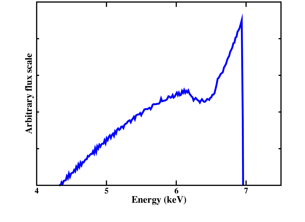
Figure 14: The predicted line profile Dauser10 from an intrinsically narrow Fe K$\alpha$ emission line at $6.4$ keV that has been altered by Doppler broadening, special relativistic beaming, and general relativistic effects.

In many ways, the study of “blurred’ reflection (e.g. Miller07 ; Bambi21 ; Reynolds21 ) is best suited for broadband spectroscopy and variability. For example, even in the “clean” Fe K region, the breadth of the Fe K$\alpha$ can extend over several keV (Figure 14). The expanse of the reflection spectrum can overwhelm emission from other regions like distant reflection and even the primary continuum (e.g. Fabian09 ; Ponti10 ). This can be even more daunting when discerning relativistic features among the warm absorbers at low energy (e.g. steenbrugge09 ). Great advances have been made utilizing XMM-Newton and NuSTAR together to produce spectra between $0.3-79$ keV (e.g. Wilkins15 ; Jiang18 ; Walton20 ; Wilkins22 ). Relativistic, ionised reflection can also produce signatures in timing data generated from reverberation delays between the continuum and reflecting components (e.g. Zoghbi10 ; Zoghbi12 ). There is massive potential in discerning the geometry and environment in the inner few gravitational radii from the study of relativistic reflection (e.g. Alston20 ; Reynolds21 ; Wilkins22 ).

A major challenge for realizing this potential is that alternate models like the two-coronae scenario (e.g. wc1 ; wc2 ; Ballantyne20 ) and (ionised) partial covering (e.g. Holt80 ; Tanaka04 ) can mimic the appearance of relativistic reflection. High-resolution spectroscopy can provide some headway in breaking this degeneracy. In Figure 15, an intrinsic power law spectrum modified by ionised partial covering is simulated for a $100$ ks observation with XRISM. The data are then fitted with blurred reflection to show that XRISM can potential reveal narrow absorption features originating from the ionised partial covering material.

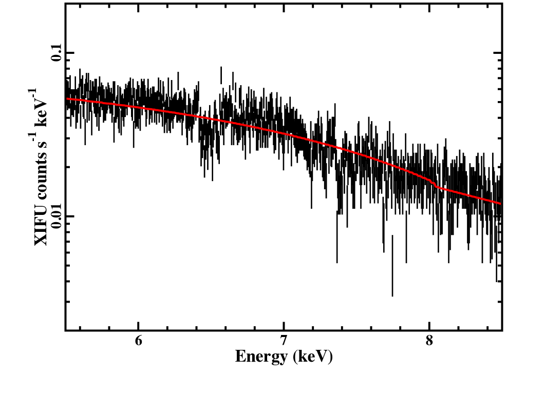
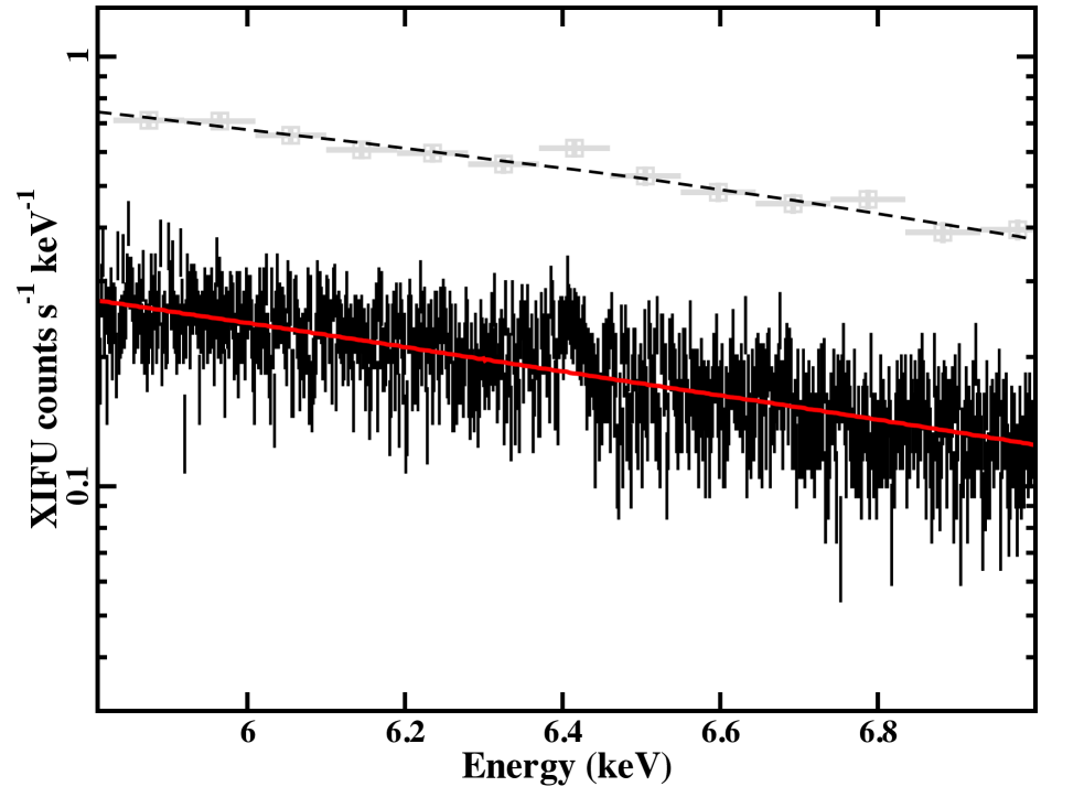
Figure 15: Upper panel: A $100$ ks XRISM-Resolve simulation of a power law modified by ionised partial covering and fitted with blurred reflection. Narrow absorption features from the absorbing material should be evident in XRISM data. Lower panel: A $100$ ks Athena-XIFU simulation (black data) of a combined strong blurred reflector with a reflection fraction $\mathcal{R}=3$ and a weak distant reflector with $\mathcal{R}=0.3$, fitted with a single blurred reflector. The weak distant emitter becomes evident in the Athena data. A simulation for the EPIC-pn is shown in grey and is scaled for comparison. The $2-10$ keV flux is $10^{-11}\rm~{}erg~{}cm^{-2}~{}s^{-1}$ in both panels and the data are optimally binned optbin .

Enhanced spectral resolution can also disentangle blurred reflection from other components. In Figure 15, a weak distant reflector with a reflection fraction $\mathcal{R}=0.3$ is added to a strong blurred reflector with $\mathcal{R}=3$ and simulated for a $100$ ks Athena observation. When fitted with blurred reflection alone, the weak narrow Fe K$\alpha$ component from distant material is uncovered in the data.

0.4 The nature of ultrafast outflows

For understanding ultrafast outflows (UFOs), the discovery space that will become accessible through high-resolution X-ray spectroscopy will be tremendous. Various processes tied to the accretion mechanism can generate outflows from the disc (e.g. Murray95 ; Begelman83 ; BP82 ). If these outflows have sufficient energy to escape the inner kilo-parsec of the host galaxy, they can significantly impact star formation and abundances in the interstellar medium.

AGN feedback (e.g. Begelman04 ; King10 ; Fabian12 ) will be important to galaxy evolution if the kinetic luminosity (Eq. 1) of the wind deposits into the host galaxy approximately $0.5\%-5\%$ of the AGN bolometric luminosity SR98 ; DiMatteo05 ; SH05 ; HE10 ; KP15 . Winds that originate at large distances from the black hole, for example from the torus or WAs, might be expected to have important effects on the host galaxy, however, these are rather slow-moving and may not carry sufficient kinetic luminosity or travel significant distances to influence the galaxy Crenshaw12 ; Fischer17 . To this end, the highly blueshifted absorption features evident in some AGN X-ray spectra (Figure 16), that are indicators of the so-called ultrafast outflows – highly ionised material ejected from the black hole vicinity at substantial fractions of the speed of light – might serve as the mechanism for delivering energy to the galaxy. Since $L_{KE}\propto v_{r}^{3}$, these fast winds can potentially deposit the most amount of energy into the surroundings and alter galaxy evolution.

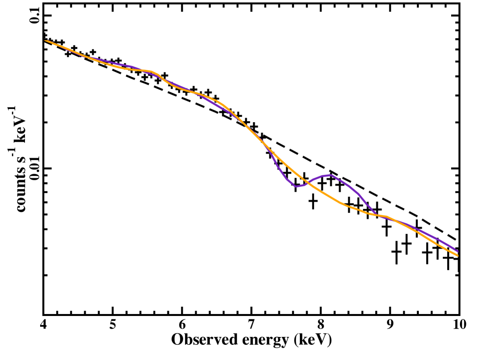
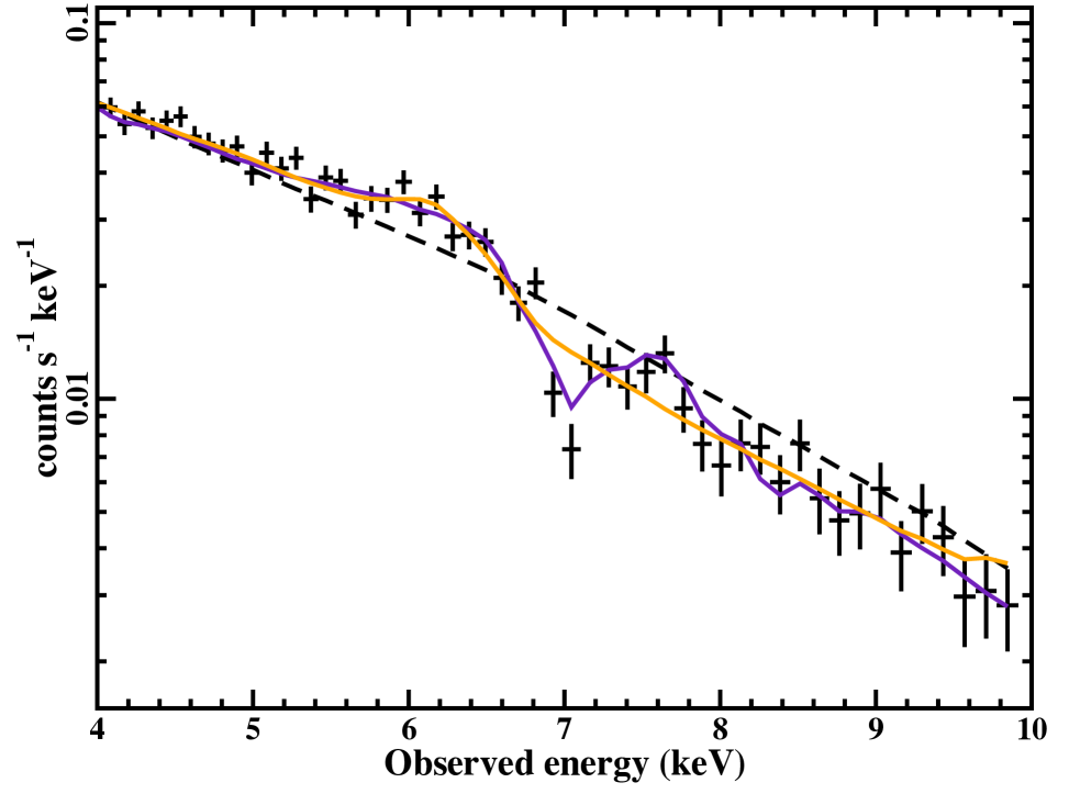
Figure 16: EPIC-pn data from XMM-Newton observations of PDS 456 (upper panel; obsid:07210401) and PG $1211+143$ (lower panel; obsid:01126101). In both cases, a single power law (black dashed curve) leaves absorption features above $7$ keV. The MHD-driven wind (mhdwind) Fukumura22 and line-driven wind (fast32rg) Matzeu22 , represented by the orange and purple curves, respectively, reproduce the CCD data equally well. Note, since mhdwind does not currently account for scattered emission self-consistently, a Gaussian emission profile is included for more direct comparison to fast32rg.

0.4.1 UFO characteristics

XMM-Newton, Chandra, and Suzaku ushered in an era of high throughput spectroscopy in the Fe K$\alpha$ band between $5-10$ keV. Early observations revealed absorption-like features above $7$ keV (rest-frame) in the distant ($z=3.91$) lensed quasar APM $08279+5255$ Chartas02 , the nearby ($z=0.184$) luminous quasar PDS 456 Reeves03 , and the narrow-line Seyfert 1 quasar, PG $1211+143$ Pounds03 . Attributed to K-shell absorption lines from Fe xxv (He-like, $6.70$ keV) and Fe xxvi (H-like, $6.97$ keV) implies relativistic velocities between $0.1-0.3$c.

Sample studies Cappi06 ; Tombesi10a ; Gofford13 ; Igo20 detect possible features with equivalent widths between $15-100$ eV in approximately $30\%-40\%$ of sources. This population includes jetted Tombesi10b and non-jetted AGN, as well as sources radiating at sub-Eddington and high-Eddington Pounds03 ; Hagino16 ; Parker17 values. The high ionisation state of iron and depth of the absorption features implies high ionisation parameters of $\rm log(\xi/erg~{}cm~{}s^{-1})\sim 3-6$ and column densities of $\rm log(N_{H}/cm^{-2})\sim 22-24$ Tombesi11 ; Gofford13 . The high detection rate indicates the covering factor ($\Omega$) of the wind is large. Indeed, in PDS 456 an average solid angle of $\Omega\sim 3.2\pi$ is estimated Nardini15 . In general, the application of P-Cygni profiles to simultaneously fit the absorption and emission from the wind imply it might be close to spherically symmetric Done07 ; Nardini15 ; Reeves19 .

UFO signatures have been reported in high-resolution grating data at lower energies between $0.3-2$ keV Longinotti15 ; Boissay19 ; Pounds03 ; Gupta13 ; Gupta15 ; Reeves20 . The co-existence of slow-moving warm absorbers and ultrafast outflows Rogantini22 ; Pinto18 ; Parker17 ; Xu21 raise the question if these are different phases of the same stratified flow Serafinelli19 . It is not yet clear if the AMD (Section 0.2) can be described by an outflowing medium that is continuous, patchy, or in pressure equilibrium Behar09 ; Krongold03 ; Detmers11 .

UFO features are significantly variable in equivalent width and velocities on all time scales down to hours Igo20 ; Parker17 ; Pinto18 ; Gallo19 ; Matzeu17 ; Reeves19 . In some cases, these variations may arise from the wind responding to luminosity changes or they might be intrinsic to the launching mechanism (Section 0.4.2). In these cases, variability studies will render a profound understanding of the wind and central engine. Ascertaining the response time of the wind to changes in the ionising continuum reveals the wind density ($n$) since the recombination time is inversely proportional to $n$ (Eq. 6). The distance to the wind then follows since the ionisation parameter and luminosity are measured in the spectrum (i.e. $r=\frac{L_{ion}}{n\xi}$, from Eq. 4).

It is still not completely possible to rule out that some wind features are consistent with random noise events. In some cases, the wind features are based on the detection of a single absorption feature whose significance can depend on the continuum model and spectral binning. As illustrated in the Astro-H White paper on AGN winds Kaastra14 , the detection of two lines with a null hypothesis significance of $p_{1}$ and $p_{2}$ will elevate the significance of the wind to $p_{1}\times p_{2}$. With the potential to discern blended lines and distinguish weak features, high-resolution spectroscopy can better determine the occurrence rate of winds in AGN that is important for determining the wind geometry.

Figure 17 provides a demonstration of how line detection and line width will be significantly improved upon in the high-resolution era. In the example, the H- and He-like iron lines have a turbulent velocity of $v_{turb}=500$ km s^-1. The line is undetected in the $100$ ks pn observation, but the Fe xxvi is significantly detected in the $100$ ks XRISM-Resolve spectrum despite a smaller effective area. Moreover, the Resolve data easily distinguishes from a high turbulent velocity of $5000$ km s^-1 and even from much more comparable velocities of $\sim 1000$ km s^-1.

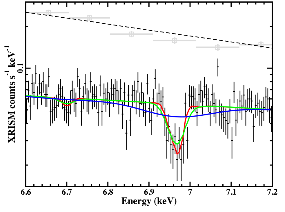
Figure 17: Simulated spectra of a photoionised plasma with $\rm log(N_{H}/cm^{-2})=23$, $\rm log(\xi/erg~{}cm~{}s^{-1})=4$ and $v_{turb}=500$ km s^-1. Both the EPIC-pn (grey) and XRISM-Resolve data (black) are based on $2-10$ keV brightness of $\sim 10^{-11}\rm erg~{}cm^{-2}~{}s^{-1}$ and an exposure of $100$ ks. The pn data are well fitted with a single power law. The Fe xxvi is significantly detected in the XRISM data and models with different turbulent velocities of $500$ km s^-1 (red), $1000$ km s^-1 (green), and $5000$ km s^-1 (blue) can be meaningfully examined. The pn spectrum is scaled for comparison. The data are optimally binned optbin .

0.4.2 The wind origin

The rapid variability, high degree of ionisation, and relativistic velocities all point to UFO features originating close to the black hole. The inner accretion disc provides a natural environment for generating outflows in addition to the inward transport of matter. The mechanisms by which winds are launched from an accretion disc are from (i) thermal (gas) pressure, (ii) radiation pressure, and (iii) magnetic fields. Which mechanism dominates depends on a number of factors including the degree of ionisation in the wind and the geometry of the system (see Figure 1).

Thermal driven winds

The upper layer of the accretion disc will expand if it is heated to the Compton temperature by the X-rays coming from the inner region. If the rate of expansion exceeds the escape velocity ($v_{esc}=\sqrt{2GM_{BH}/r}$) at a given radius ($r$), a thermal wind will be produced Begelman83 . Thermal winds are commonly employed in stellar mass black holes Done18 ; Tomaru23 . Simulations show that thermal winds reach speeds of only $200-300$ km s^-1 because they are launched ballistically from the outer accretion disc (e.g. HP15 ; Higginbottom17 ). Such winds are inadequate for explaining the UFO phenomenon in AGN.

Radiative driven winds

Radiation pressure from the accretion disc can launch a wind Murray95 ; Proga00 ; Proga04 ; KB01 . This is best exemplified in broad absorption line (BAL) quasars that show broad UV absorption lines from, for example, C iv and N v, outflowing at velocities $\sim 10,000\rm km~{}s^{-1}$ (e.g. Turnshek84 ; Weymann91 ; Allen11 ).

If the gas is highly or completely ionised, Thomson and Compton scattering can be sufficient to power the wind. This continuum-driving will be important in high luminosity systems radiating at values close to Eddington KP03 . However, winds are commonly seen in sub-Eddington systems. In these cases, line-driving will be more consequential.

In the line-driving scenario, the photoabsorption cross-section is larger than the electron scattering cross-section. The opacity in the absorption lines serves as a force multiplier to enhance the effects of radiation pressure Castor75 ; Proga00 ; KB01 ; Dannen19 . In this way, sub-Eddington sources can efficiently launch fast winds of weakly ionised material as is seen in BAL quasars. However, the effects of the force multiplier are lost at $\rm log(\xi/erg~{}cm~{}s^{-1})>3$ Dannen19 even though ionisation parameters of $\rm log(\xi/erg~{}cm~{}s^{-1})>4$ are required to describe the spectral features seen in X-ray winds. The ionisation of the gas likely occurs after the wind is launched, once it reaches a sufficient height above the disc (above the shielding failed wind; see Figure 1) to be exposed to the central X-rays Proga04 ; Higginbottom14 ; Hagino15 ; Nomura17 ; Nomura20 ; Mizumoto21 .

The observer looking down the line-driven wind funnel will see a large range of velocities. The slow wind at large distance is generally moving along the line-of-sight, but the fast winds will move on streamlines that are increasingly slanted closer to the origin (Figure 18). This produces an absorption line profile with a sharp blue edge and extended red tail Knigge95 ; LK02 ; Sim08 ; Hagino15 ; Matzeu22 . Such a profile is depicted in Figure 18 using the fast32rg disc wind model Matzeu22 ; Sim08 ; Sim10 and can be compared to the MHD-driven wind profiles in Section 0.4.2.

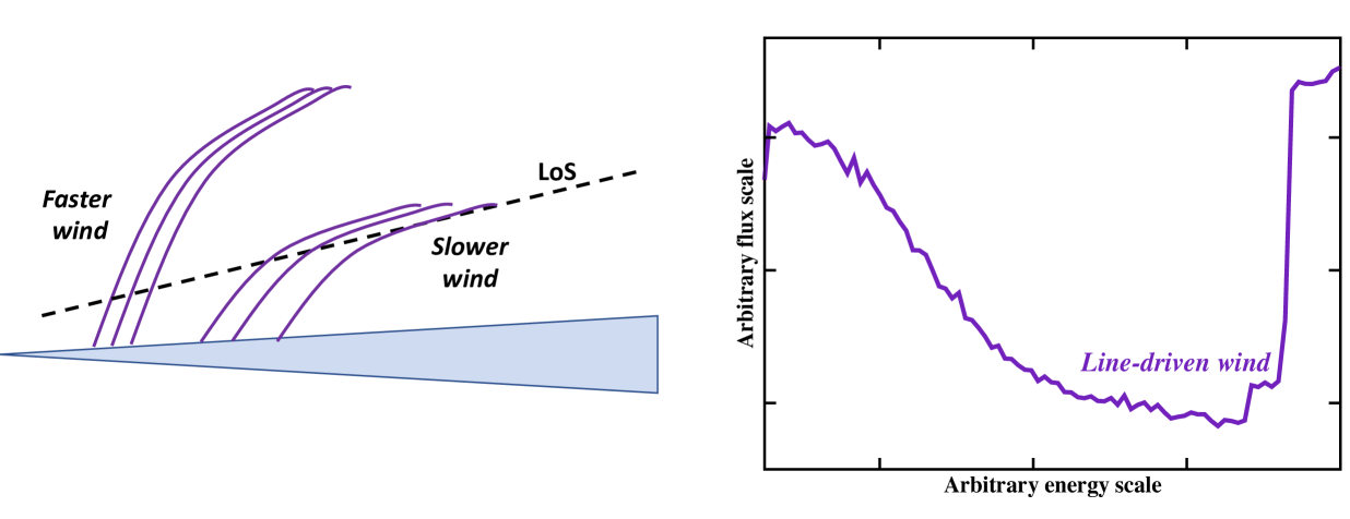
Figure 18: Left: The faster streamlines originating closer to the X-ray source will be more vertical compared to those of the slower wind at larger distances. Right: The scenario results in a line profile with a sharp blue edge and an extend red wing, which is a signature of the line-driven wind models.

Magnetic driven winds

An outflow driven by magnetohydrodynamics (MHD) in the accretion disc is widely expected BP82 ; CL94 ; Fukumura10a ; Fukumura10b ; Kazanas12 . In many sub-Eddington sources that possess UFOs, the force multiplier is small (i.e. the material is too highly ionised) to radiatively accelerate the wind Kraemer18 . MHD winds can naturally explain the high velocity of highly ionised material without the need for line-driving.

The wind will be launched from a continuous region over a large area of the accretion disc. The wind density will fall with increasing distance. The ionised gas will be accelerated in the poloidal magnetic field by magnetic-centrifugal and magnetic pressure forces BP82 ; CL94 ; Fukumura10a ; Fukumura22 ; Kazanas12 . The faster gas will originate closer to the black hole. Consequently, the fastest gas is also the most ionised gas. The line profile will depend on the velocity gradient along the line-of-sight and this can yield a characteristic line profile for MHD-driven winds when combined with the photoionisation balance Fukumura22 .

For a given ion, the column density will depend on the density gradient. At the peak column density the optical depth in the line is maximum. Moving toward a lower ionisation parameter (i.e. increasing distance from the ionising source) the column density drops rapidly producing a sharp red edge in the line. The column density drops off more gradually as the ionisation parameter increases (i.e. decreasing distance) such that a blue wing forms in the line. An example of the opacity in the Fe xxvi line for an adopted AMD is shown in the right panel of Figure 19 (data kindly provided by K. Fukumura). Using the mhdwind disc wind model Fukumura22 , it is seen that the MHD-driven wind will produce a line profile that replicates the same behaviour (Figure 19, left panel). This can be compared to the red asymmetry that is generated in a line-driven wind (see Figure 18).

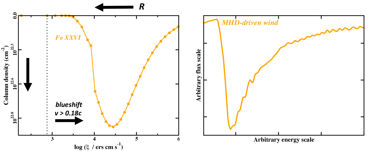
Figure 19: Left: The calculated column density (inverted on the vertical axis) as a function of ionisation parameter in the Fe xxvi line for an adopted AMD (data provide courtesy of K. Fukumura). The ionisation parameter and velocity decrease with increasing distance ($R$) from the primary X-rays source. Right: The sharp red edge and extended blue wing in the $\rm N_{H}-\xi$ relation is replicated in the absorption line profile produced by an MHD-driven wind.

Distinguishing the winds with high resolution spectroscopy

Despite the striking differences evident in the line profiles (Figures 17,  18, and  19), the CCD resolution afforded by current observatories is insufficient to distinguish wind models. As shown in Figure 16, the MHD- and radiative-driven winds describe XMM-Newton data of PDS 456 and PG 1211+143 relatively well.

The power of the high spectral resolution and large effective area that will be delivered by Athena-XIFU is on display in Figure 20. Here, the best-fit MHD-driven wind model (mhdwind) used to describe the EPIC-pn data (Figure 16) is simulated for a $100\rm~{}ks$ observation with the Athena-XIFU. The XIFU data cannot be well fitted with the line-driven wind model (fast32rg) because of the different line profiles (Figure 20).

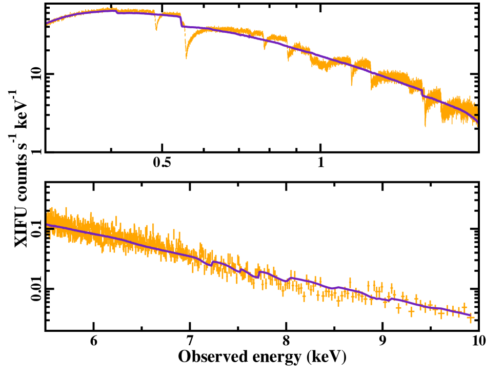
Figure 20: Simulated Athena-XIFU spectrum of PDS 456 ($100\rm~{}ks$) assuming the best-fit MHD-wind (mhdwind) shown in Figure 16. The data are then fitted (purple curve) with the line-driven wind model (fast32rg). The line profiles can be clearly distinguished with Athena revealing the nature of the launching mechanism.

0.4.3 A windless alternative?

Less fashionable, but equally important, is to consider alternative interpretations for the UFO features seen in X-ray spectra. In 2011, Gallo & Fabian GF11 proposed that the blueshifted absorption features might not be due to outflows, but simply arising from low density, ionised gas on the surface of the orbiting inner disc. In this scenario, the absorption feature is effectively an inverted disc line Fabian89 ; Laor that is modified by orbital motions and relativity, and is imprinted on the reflection spectrum. Orbital velocities within $10~{}R_{G}$ are more than sufficient to reproduce the blueshifts seen in UFOs features GF11 .

The model was shown to fit the spectra of PG 1211+143 (Figure 21) GF13 and IRAS $13224-3809$ Fabian20 . For IRAS $13224-3809$, the long, near continuous observations permitted variability studies of the UFO features Parker17 ; Jiang18 ; Pinto18 . The manner in which the features were stronger in the low-flux state and disappeared when the AGN was bright was attributed to overionising the gas in the high-flux state. In the disc-absorption scenario, the variability was consistent with the increased reflection fraction at low flux levels Fabian20 .

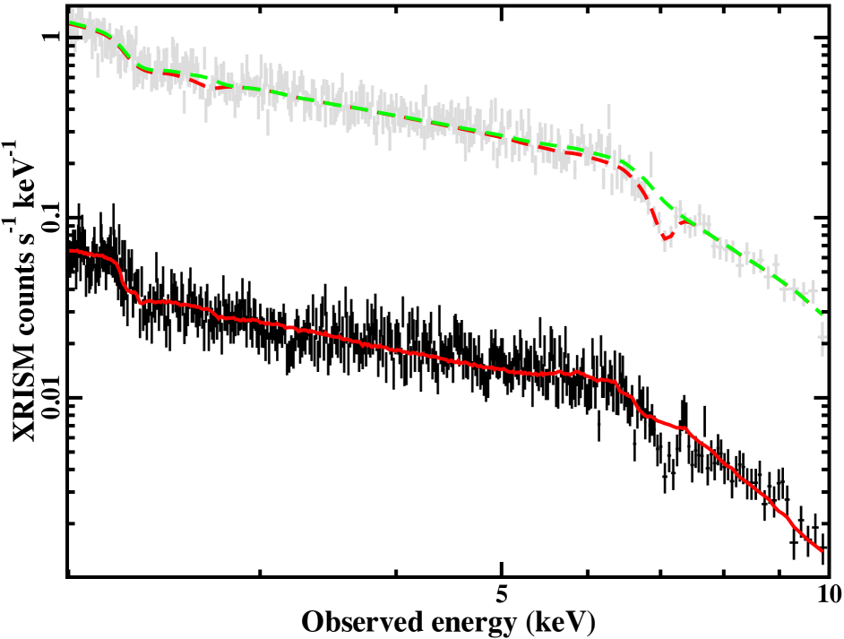
Figure 21: The disc-line absorption model fitted to the $2-10~{}\rm keV$ XMM-Newton pn data (grey) of PG $1211+143$. The green dashed line is a blurred ionised reflection fit to the spectrum. The red dashed curve shows the fit to the data when including an inverted disc line originating beyond $6~{}R_{G}$. The figure is reproduced with permission from GF13 . The model is simulated for a $100\rm~{}ks$ XRISM-Resolve observation (black) and fitted with a line-driven wind model with no blurred reflection (solid red curve). The wind model fits the redward emission well with a P-Cygni profile, but is unable to simultaneously describe the absorption. The alternative disc-line absorption model should be testable with XRISM.

This alternative model can be tested with high-resolution spectroscopy. A $100\rm~{}ks$ XRISM-Resolve simulation of PG $1211+143$ is shown in Figure 21. When the simulated data are fitted with a line-driven wind model with no blurred reflection, the redward excess and blueshifted absorption cannot be simultaneously reproduced. Such a scenario cannot replace the wind scenario in all cases but might be viable for AGN exhibiting strong blurred reflection like some narrow-line Seyfert 1 galaxies Gallo18 . This model can be scrutinized with XRISM and Athena.

0.4.4 Progress and caveats

High-resolution X-rays spectroscopy will carry the massive potential to enhance our understanding of ultrafast outflows in AGN. With XRISM, Arcus, and Athena we will truly begin probing the origins, physics, and mechanisms at work in winds; and finally, test alternative models. Not only will this improve our understanding of UFOs themselves, but better our knowledge of AGN physics on the black hole scales and AGN feedback on galactic scales.

High-resolution spectroscopy will expose our misunderstandings. The current wind models are incredibly sophisticated, but are incomplete as they are based on simplifying assumptions, limited understanding, and finite computational power. Line profiles will depend on a number of factors, for example, the slope of the AMD. Even with high resolution, in some situations the different launching mechanisms might produce similar profiles Fukumura22 . The reader is advised to understand the assumptions and limitations of each model before employing them in research.

The physical situation will undoubtedly be much more complex. There is no reason that hybrid winds, which are combinations of thermal, magnetic and radiative, cannot co-exist in a given AGN Everett05 . Likewise, the blurred reflection will also complicate modelling Parker22 , and both the intrinsic AGN and wind can be simultaneously varying on different time scales.

0.5 Conclusion

The AGN community has benefited immensely from XMM-Newton, Chandra, and other great X-ray observatories over the past 20 years. Many of these instruments will be producing excellent science for years to come. It is because of the tremendous success we have had with these instruments that the community can move forward with an eye on high resolution spectroscopy.

The launch of XRISM is imminent. This will be followed by the launch of an Athena-like mission (NewAthena) in the early or mid-2030s, covering the same pass band with even sharper resolution and higher sensitivity. In between, mission concepts such as Arcus may provide particularly high resolution grating spectroscopy below 1 keV, potentially simultaneously with UV spectroscopy, providing pristine line profiles to perform different density diagnostic tests, the detection of metastable levels, and time-resolved spectroscopy.

Assuming that the calorimeter aboard XRISM will operate for ten years, what are some optimistic goals for our understanding of AGN? And what are some equivalent goals for the more advanced missions that will follow XRISM?

The sensitivity of XRISM should clearly determine the demographics of both slow X-ray winds, and UFOs in bright, local Seyferts. We should learn if some sources display particularly line-rich spectra because they afford a fortuitous viewing angle, because their Eddington fraction is just right, or because their wind components have fortuitous ionisation levels. It is particularly important to understand the demographics of wind feedback as a function of Eddington fraction and XRISM will begin examining this for local Seyferts. If XRISM finds that UFOs provide insufficient feedback in the Seyfert phase, this does not preclude a larger role for winds at higher Eddington fractions. Athena will make it possible to extend detailed wind studies to quasars at modest red-shifts, and to local sources with lower Eddington fractions, and thus answer this key question.

In a subset of the brightest Seyferts, XRISM should be able to extend the range in ionisation over which AMDs are constructed by two orders of magnitude, offering an improved understanding of wind driving mechanisms. In the same subset, ionisation time scales should reveal gas densities, and therefore the absorption radius in the given wind zone, providing an independent angle on wind-driving mechanisms.

Since new reverberation studies suggest that the innermost wall of the “torus” is only a factor of a few more distant from the central engine than the optical BLR, few composite narrow Fe K$\alpha$ emission line profiles might be expected in XRISM spectra. However, observations of bright Seyferts should clearly reveal the narrow Fe K$\alpha$ line production region and its relationship to the BLR and torus. In a subset of the brightest Seyferts, reverberation mapping may offer an independent view on this problem, as well as independent constraints on black hole masses. If the disk is warped between the ISCO and the BLR owing to a misalignment of the disk with the black hole spin vector, resulting in “extra” reflecting area per unit radius, XRISM may also be able to reveal hints of this structure. In the longer term, the added sensitivity afforded by Athena should be able to test related theories in a much larger set of systems.

The epoch of high-resolution X-ray spectroscopy is upon us. For AGN, this is an exciting era that is full of massive potential for uncovering the ins and outs of black hole accretion.

- (1) J. T. Allen, P. C. Hewett, N. Maddox, G. T. Richards, & V. Belokurov, MNRAS 410, 860-884 (2011) doi:10.1111/j.1365-2966.2010.17489.x [arXiv:1007.3991]
- (2) W. N. Alston, A. C. Fabian, E. Kara, et al., NatAs 4, 597-602 (2020) doi:10.1038/s41550-019-1002-x [arXiv:2001.06454]
- (3) C. Andonie, F. E. Bauer, R. Carraro, et al., A&A 664, A46 (2022) doi:10.1051/0004-6361/202142473 [arXiv:2204.09469]
- (4) R. Antonucci, ARA&A 31, 473-521 (1993) doi:10.1146/annurev.aa.31.090193.002353
- (5) N. Arav, C. Chamberlain, G. A. Kriss, et al., A&A 577, A37 (2015) doi:10.1051/0004-6361/20142530210.48550/arXiv.1411.2157 [arXiv:1411.2157]
- (6) N. Arav, M. Moe, E. Costantini, et al., ApJ 681, 954-964 (2008) doi:10.1086/588651 [arXiv:0807.0228]
- (7) S. A. Balbus & J. F. Hawley, ApJ 376, 214 (1991) doi:10.1086/170270
- (8) J. Baldwin, G. Ferland, K. Korista, & D. Verner, ApJL 455, L119 (1995) doi:10.1086/309827 [arXiv:astro-ph/9510080]
- (9) D. R. Ballantyne, MNRAS 491, 3553-3561 (2020) doi:10.1093/mnras/stz3294 [arXiv:1911.10029]
- (10) D. R. Ballantyne, R. R. Ross, & A. C. Fabian, MNRAS 327, 10-22 (2001) doi:10.1046/j.1365-8711.2001.04432.x [arXiv:astro-ph/0102040]
- (11) C. Bambi, L. W. Brenneman, T. Dauser, et al., SSRv 217, 65 (2021) doi:10.1007/s11214-021-00841-8 [arXiv:2011.04792]
- (12) W. Bambynek, B. Crasemann, R. W. Fink, et al., Reviews of Modern Physics, 44, 716-813 (1972)
- (13) D. Barret, T. Lam Trong, J.-W. den Herder, et al., SPIE 10699, 106991G (2018) doi:10.1117/12.2312409 [arXiv:1807.06092]
- (14) M. A. Bautista, C. Mendoza, T. R. Kallman, & P. Palmeri, A&A 403, 339-355 (2003) doi:10.1051/0004-6361:20030367 [arXiv:astro-ph/0207323]
- (15) M. A. Bautista, C. Mendoza, T. R. Kallman, & P. Palmeri, A&A 418, 1171-1178 (2004) doi:10.1051/0004-6361:20034198
- (16) M. C. Begelman, cbhg.symp 374 (2004) doi: [arXiv:astro-ph/0303040]
- (17) M. C. Begelman, C. F. McKee, & G. A. Shields, ApJ 271, 70-88 (1983) doi:10.1086/161178
- (18) E. Behar, ApJ 703, 1346-1351 (2009) doi:10.1088/0004-637X/703/2/1346 [arXiv:0908.0539]
- (19) E. Behar, M. Sako, & S. M. Kahn, ApJ 563, 497-504 (2001) doi:10.1086/323966 [arXiv:astro-ph/0109314]
- (20) M. C. Bentz, P. R. Williams, & T. Treu, ApJ 934, 168 (2022) doi:10.3847/1538-4357/ac7c0a [arXiv:2206.03513]
- (21) S. Bianchi, M. Guainazzi, G. Matt, N. Fonseca Bonilla, & G. Ponti, A&A 495, 421-430 (2009) doi:10.1051/0004-6361:200810620 [arXiv:0811.1126]
- (22) R. D. Blandford & D. G. Payne, MNRAS 199, 883-903 (1982) doi:10.1093/mnras/199.4.883
- (23) J. Bland-Hawthorn, S. L. Lumsden, G. M. Voit, G. N. Cecil, & J. C. Weisheit, Ap&SS 248, 177-190 (1997) doi:10.1023/A:1000525513140 [arXiv:astro-ph/9706211]
- (24) A. J. Blustin, M. J. Page, S. V. Fuerst, G. Branduardi-Raymont, & C. E. Ashton, A&A 431, 111-125 (2005) doi:10.1051/0004-6361:20041775 [arXiv:astro-ph/0411297]
- (25) R. Boissay-Malaquin, A. Danehkar, H. L. Marshall, & M. A. Nowak, ApJ 873, 29 (2019) doi:10.3847/1538-4357/ab0082 [arXiv:1901.06641]
- (26) T. Boller, W. N. Brandt, & H. Fink, A&A 305, 53 (1996) doi:10.48550/arXiv.astro-ph/9504093 [arXiv:astro-ph/9504093]
- (27) W. N. Brandt, S. Mathur, & M. Elvis, MNRAS 285, L25-L30 (1997) doi:10.1093/mnras/285.3.L2510.48550/arXiv.astro-ph/9703100 [arXiv:astro-ph/9703100]
- (28) H. Brunner, T. Liu, G. Lamer, et al., A&A 661, A1 (2022) doi:10.1051/0004-6361/202141266 [arXiv:2106.14517]
- (29) M. Cappi, AN 327, 1012 (2006) doi:10.1002/asna.200610639 [arXiv:astro-ph/0610117]
- (30) J. I. Castor, D. C. Abbott, & R. I. Klein, ApJ 195, 157-174 (1975) doi:10.1086/153315
- (31) S. Chakravorty, A. K. Kembhavi, M. Elvis, & G. Ferland, MNRAS 393, 83-98 (2009) doi:10.1111/j.1365-2966.2008.14249.x10.48550/arXiv.0811.2404 [arXiv:0811.2404]
- (32) S. Chakravorty, R. Misra, M. Elvis, A. K. Kembhavi, & G. Ferland, MNRAS 422, 637-651 (2012) doi:10.1111/j.1365-2966.2012.20641.x10.48550/arXiv.1201.5435 [arXiv:1201.5435]
- (33) G. Chartas, W. N. Brandt, S. C. Gallagher, & G. P. Garmire, ApJ 579, 169-175 (2002) doi:10.1086/342744 [arXiv:astro-ph/0207196]
- (34) J. Contopoulos & R. V. E. Lovelace, ApJ 429, 139 (1994) doi:10.1086/174307
- (35) E. Costantini, SSRv 157, 265-277 (2010) doi:10.1007/s11214-010-9706-310.48550/arXiv.1011.2384 [arXiv:1011.2384]
- (36) E. Costantini, J. S. Kaastra, N. Arav, et al., A&A 461, 121-134 (2007) doi:10.1051/0004-6361:20065390 [arXiv:astro-ph/0609385]
- (37) E. Costantini, J. S. Kaastra, K. Korista, et al., A&A 512, A25 (2010) doi:10.1051/0004-6361/200912555 [arXiv:1001.2712]
- (38) E. Costantini, G. Kriss, J. S. Kaastra, et al., A&A 595, A106 (2016) doi:10.1051/0004-6361/201527956 [arXiv:1606.06579]
- (39) E. Costantini, F. Nicastro, A. Fruscione, et al., ApJ 544, 283-292 (2000) doi:10.1086/31720010.48550/arXiv.astro-ph/0007158 [arXiv:astro-ph/0007158]
- (40) D. M. Crenshaw & S. B. Kraemer, ApJ 753, 75 (2012) doi:10.1088/0004-637X/753/1/75 [arXiv:1204.6694]
- (41) D. M. Crenshaw, S. B. Kraemer, J. R. Gabel, et al., ApJ 594, 116-127 (2003) doi:10.1086/37679210.48550/arXiv.astro-ph/0305154 [arXiv:astro-ph/0305154]
- (42) B. Czerny, M. Nikołajuk, A. Różańska, et al., A&A 412, 317-329 (2003) doi:10.1051/0004-6361:20031441 [arXiv:astro-ph/0309242]
- (43) R. C. Dannen, D. Proga, T. R. Kallman, & T. Waters, ApJ 882, 99 (2019) doi:10.3847/1538-4357/ab340b [arXiv:1812.01773]
- (44) T. Dauser, J. Wilms, C. S. Reynolds, & L. W. Brenneman, MNRAS 409, 1534-1540 (2010) doi:10.1111/j.1365-2966.2010.17393.x [arXiv:1007.4937]
- (45) M. Dehghanian, G. J. Ferland, B. M. Peterson, et al., ApJL 882, L30 (2019) doi:10.3847/2041-8213/ab3d4110.48550/arXiv.1908.07686 [arXiv:1908.07686]
- (46) R. G. Detmers, J. S. Kaastra, K. C. Steenbrugge, et al., A&A 534, A38 (2011) doi:10.1051/0004-6361/201116899 [arXiv:1107.0658]
- (47) L. Di Gesu & E. Costantini, A&A 594, A88 (2016) doi:10.1051/0004-6361/20162867010.48550/arXiv.1607.01943 [arXiv:1607.01943]
- (48) L. Di Gesu, E. Costantini, N. Arav, et al., A&A 556, A94 (2013) doi:10.1051/0004-6361/201321416 [arXiv:1305.6232]
- (49) L. Di Gesu, E. Costantini, J. Ebrero, et al., A&A 579, A42 (2015) doi:10.1051/0004-6361/201525934 [arXiv:1505.02562]
- (50) L. Di Gesu, E. Costantini, E. Piconcelli, et al., A&A 563, A95 (2014) doi:10.1051/0004-6361/201322916 [arXiv:1401.5614]
- (51) T. Di Matteo, V. Springel, & L. Hernquist, Natur 433, 604-607 (2005) doi:10.1038/nature03335 [arXiv:astro-ph/0502199]
- (52) C. Done, M. A. Sobolewska, M. Gierliński, & N. J. Schurch, MNRAS 374, L15-L19 (2007) doi:10.1111/j.1745-3933.2006.00255.x [arXiv:astro-ph/0610078]
- (53) C. Done, R. Tomaru, & T. Takahashi, MNRAS 473, 838-848 (2018) doi:10.1093/mnras/stx2400 [arXiv:1612.09377]
- (54) J. Ebrero, V. Domček, G. A. Kriss, & J. S. Kaastra, A&A 653, A125 (2021) doi:10.1051/0004-6361/202040045 [arXiv:2107.05676]
- (55) J. Ebrero, G. A. Kriss, J. S. Kaastra, & J. C. Ely, A&A 586, A72 (2016) doi:10.1051/0004-6361/20152749510.48550/arXiv.1511.07169 [arXiv:1511.07169]
- (56) D. Edmonds, B. Borguet, N. Arav, et al., ApJ 739, 7 (2011) doi:10.1088/0004-637X/739/1/7
- (57) J. E. Everett, ApJ 631, 689-706 (2005) doi:10.1086/432678 [arXiv:astro-ph/0506321]
- (58) A. C. Fabian, ARA&A 50, 455-489 (2012) doi:10.1146/annurev-astro-081811-125521 [arXiv:1204.4114]
- (59) A. C. Fabian, M. J. Rees, L. Stella, & N. E. White, MNRAS 238, 729-736 (1989) doi:10.1093/mnras/238.3.729
- (60) A. C. Fabian, C. S. Reynolds, J. Jiang, et al., MNRAS 493, 2518-2522 (2020) doi:10.1093/mnras/staa482 [arXiv:2002.06388]
- (61) A. C. Fabian, A. Zoghbi, R. R. Ross, et al., Natur 459, 540-542 (2009) doi:10.1038/nature08007
- (62) L. Ferrarese & D. Merritt, ApJL 539, L9-L12 (2000) doi:10.1086/312838 [arXiv:astro-ph/0006053]
- (63) T. C. Fischer, C. Machuca, M. R. Diniz, et al., ApJ 834, 30 (2017) doi:10.3847/1538-4357/834/1/30 [arXiv:1609.08927]
- (64) K. Fukumura, M. Dadina, G. Matzeu, et al., ApJ 940, 6 (2022) doi:10.3847/1538-4357/ac9388 [arXiv:2205.08894]
- (65) K. Fukumura, D. Kazanas, I. Contopoulos, & E. Behar, ApJ 715, 636-650 (2010) doi:10.1088/0004-637X/715/1/636 [arXiv:0910.3001]
- (66) K. Fukumura, D. Kazanas, I. Contopoulos, & E. Behar, ApJL 723, L228-L232 (2010) doi:10.1088/2041-8205/723/2/L228 [arXiv:1009.5644]
- (67) K. Fukumura, F. Tombesi, D. Kazanas, et al., ApJ 805, 17 (2015) doi:10.1088/0004-637X/805/1/17 [arXiv:1503.04074]
- (68) J. R. Gabel, D. M. Crenshaw, S. B. Kraemer, et al., ApJ 583, 178-191 (2003) doi:10.1086/34509610.48550/arXiv.astro-ph/0209484 [arXiv:astro-ph/0209484]
- (69) J. R. Gabel, S. B. Kraemer, D. M. Crenshaw, et al., ApJ 631, 741-761 (2005) doi:10.1086/43268210.48550/arXiv.astro-ph/0506323 [arXiv:astro-ph/0506323]
- (70) L. C. Gallo, MNRAS 368, 479-486 (2006) doi:10.1111/j.1365-2966.2006.10137.x10.48550/arXiv.astro-ph/0602145 [arXiv:astro-ph/0602145]
- (71) L. Gallo, rnls.conf 34 (2018) doi:10.22323/1.328.0034 [arXiv:1807.09838]
- (72) L. C. Gallo & A. C. Fabian, MNRAS 418, L59-L63 (2011) doi:10.1111/j.1745-3933.2011.01143.x [arXiv:1108.5060]
- (73) L. C. Gallo & A. C. Fabian, MNRAS 434, L66-L69 (2013) doi:10.1093/mnrasl/slt080 [arXiv:1306.3404]
- (74) L. C. Gallo, A. G. Gonzalez, S. G. H. Waddell, et al., MNRAS 484, 4287-4297 (2019) doi:10.1093/mnras/stz274 [arXiv:1901.07899]
- (75) K. Gebhardt, R. Bender, G. Bower, et al., ApJL 539, L13-L16 (2000) doi:10.1086/312840 [arXiv:astro-ph/0006289]
- (76) I. M. George & A. C. Fabian, MNRAS 249, 352 (1991) doi:10.1093/mnras/249.2.352
- (77) I. M. George, T. J. Turner, H. Netzer, et al., ApJS 114, 73-120 (1998) doi:10.1086/31306710.48550/arXiv.astro-ph/9708046 [arXiv:astro-ph/9708046]
- (78) M. Giustini & D. Proga, A&A 630, A94 (2019) doi:10.1051/0004-6361/201833810 [arXiv:1904.07341]
- (79) M. Giustini & D. Proga, IAUS 356, 82-86 (2021) doi:10.1017/S1743921320002628 [arXiv:2002.07564]
- (80) J. Gofford, J. N. Reeves, F. Tombesi, et al., MNRAS 430, 60-80 (2013) doi:10.1093/mnras/sts481 [arXiv:1211.5810]
- (81) C. J. Grier, P. Martini, L. C. Watson, et al., ApJ 773, 90 (2013) doi:10.1088/0004-637X/773/2/90 [arXiv:1305.2447]
- (82) M. F. Gu, T. Holczer, E. Behar, & S. M. Kahn, ApJ 641, 1227-1232 (2006) doi:10.1086/500640 [arXiv:astro-ph/0512410]
- (83) M. F. Gu, S. M. Kahn, D. W. Savin, et al., ApJ 563, 462-471 (2001) doi:10.1086/323683
- (84) A. Gupta, S. Mathur, Y. Krongold, & F. Nicastro, ApJ 772, 66 (2013) doi:10.1088/0004-637X/772/1/66 [arXiv:1301.6139]
- (85) A. Gupta, S. Mathur, & Y. Krongold, ApJ 798, 4 (2015) doi:10.1088/0004-637X/798/1/4 [arXiv:1406.5968]
- (86) M. Gupta, M. Sikora, K. Rusinek, & G. M. Madejski, MNRAS 480, 2861-2871 (2018) doi:10.1093/mnras/sty204310.48550/arXiv.1808.07170 [arXiv:1808.07170]
- (87) K. Hagino, H. Odaka, C. Done, et al., MNRAS 446, 663-676 (2015) doi:10.1093/mnras/stu2095 [arXiv:1410.1640]
- (88) K. Hagino, H. Odaka, C. Done, et al., MNRAS 461, 3954-3963 (2016) doi:10.1093/mnras/stw1579 [arXiv:1509.05645]
- (89) J. P. Halpern, ApJ 281, 90-94 (1984) doi:10.1086/162077
- (90) N. Higginbottom & D. Proga, ApJ 807, 107 (2015) doi:10.1088/0004-637X/807/1/107 [arXiv:1504.03328]
- (91) N. Higginbottom, D. Proga, C. Knigge, et al., ApJ 789, 19 (2014) doi:10.1088/0004-637X/789/1/19 [arXiv:1402.1849]
- (92) N. Higginbottom, D. Proga, C. Knigge, & K. S. Long, ApJ 836, 42 (2017) doi:10.3847/1538-4357/836/1/42 [arXiv:1612.08996]
- (93) Hitomi Collaboration, F. Aharonian, H. Akamatsu, et al., Natur 535, 117-121 (2016) doi:10.1038/nature18627 [arXiv:1607.04487]
- (94) Hitomi Collaboration, F. Aharonian, H. Akamatsu, et al., PASJ 70, 13 (2018) doi:10.1093/pasj/psx147 [arXiv:1711.06289]
- (95) T. Holczer, E. Behar, & S. Kaspi, ApJ 663, 799-807 (2007) doi:10.1086/51841610.48550/arXiv.astro-ph/0703351 [arXiv:astro-ph/0703351]
- (96) S. S. Holt, R. F. Mushotzky, R. H. Becker, et al., ApJL 241, L13-L17 (1980) doi:10.1086/183350
- (97) P. F. Hopkins & M. Elvis, MNRAS 401, 7-14 (2010) doi:10.1111/j.1365-2966.2009.15643.x [arXiv:0904.0649]
- (98) Z. Igo, M. L. Parker, G. A. Matzeu, et al., MNRAS 493, 1088-1108 (2020) doi:10.1093/mnras/staa265 [arXiv:2001.08208]
- (99) J. Jiang, M. L. Parker, A. C. Fabian, et al., MNRAS 477, 3711-3726 (2018) doi:10.1093/mnras/sty836 [arXiv:1804.00349]
- (100) J. Jiang, D. J. Walton, A. C. Fabian, & M. L. Parker, MNRAS 483, 2958-2967 (2019) doi:10.1093/mnras/sty3228 [arXiv:1811.10932]
- (101) A. Juráňová, E. Costantini, & P. Uttley, MNRAS 510, 4225-4235 (2022) doi:10.1093/mnras/stab3731 [arXiv:2201.02640]
- (102) J. S. Kaastra & J. A. M. Bleeker, A&A 587, A151 (2016) doi:10.1051/0004-6361/201527395 [arXiv:1601.05309]
- (103) J. S. Kaastra, R. G. Detmers, M. Mehdipour, et al., A&A 539, A117 (2012) doi:10.1051/0004-6361/201118161 [arXiv:1201.1855]
- (104) J. S. Kaastra, G. A. Kriss, M. Cappi, et al., Sci 345, 64-68 (2014) doi:10.1126/science.125378710.48550/arXiv.1406.5007 [arXiv:1406.5007]
- (105) J. S. Kaastra, M. Mehdipour, E. Behar, et al., A&A 619, A112 (2018) doi:10.1051/0004-6361/201832629 [arXiv:1805.03538]
- (106) J. S. Kaastra, R. Mewe, D. A. Liedahl, S. Komossa, & A. C. Brinkman, A&A 354, L83-L86 (2000) doi: [arXiv:astro-ph/0002345]
- (107) J. S. Kaastra, R. Mewe, & H. Nieuwenhuijzen, uxsa.conf 411-414 (1996) doi:
- (108) J. S. Kaastra, A. J. J. Raassen, R. Mewe, et al., A&A 428, 57-66 (2004) doi:10.1051/0004-6361:2004143410.48550/arXiv.astro-ph/0406199 [arXiv:astro-ph/0406199]
- (109) J. S. Kaastra, Y. Terashima, T. Kallman, et al., arXiv arXiv:1412.1171 (2014) doi: [arXiv:1412.1171]
- (110) T. Kallman & M. Bautista, ApJS 133, 221-253 (2001) doi:10.1086/319184
- (111) E. S. Kammoun, J. M. Miller, M. Koss, et al., ApJ 901, 161 (2020) doi:10.3847/1538-4357/abb29f [arXiv:2007.02616]
- (112) E. Kara, M. Mehdipour, G. A. Kriss, et al., ApJ 922, 151 (2021) doi:10.3847/1538-4357/ac2159 [arXiv:2105.05840]
- (113) S. Kaspi, W. N. Brandt, H. Netzer, et al., ApJL 535, L17-L20 (2000) doi:10.1086/312697
- (114) S. Kaspi, W. N. Brandt, H. Netzer, et al., ApJ 554, 216-232 (2001) doi:10.1086/321333 [arXiv:astro-ph/0101540]
- (115) D. Kazanas, K. Fukumura, E. Behar, I. Contopoulos, & C. Shrader, AstRv 7, 92-123 (2012) doi:10.1080/21672857.2012.11519707 [arXiv:1206.5022]
- (116) N. Keshet & E. Behar, ApJ 934, 124 (2022) doi:10.3847/1538-4357/ac7c6b [arXiv:2206.15074]
- (117) A. R. King, MNRAS 402, 1516-1522 (2010) doi:10.1111/j.1365-2966.2009.16013.x [arXiv:0911.1639]
- (118) A. R. King & K. A. Pounds, MNRAS 345, 657-659 (2003) doi:10.1046/j.1365-8711.2003.06980.x [arXiv:astro-ph/0305541]
- (119) A. King & K. Pounds, ARA&A 53, 115-154 (2015) doi:10.1146/annurev-astro-082214-122316 [arXiv:1503.05206]
- (120) C. Knigge, J. A. Woods, & J. E. Drew, MNRAS 273, 225-248 (1995) doi:10.1093/mnras/273.2.225
- (121) S. Komossa, NewAR 44, 483-485 (2000) doi:10.1016/S1387-6473(00)00084-110.48550/arXiv.astro-ph/9810105 [arXiv:astro-ph/9810105]
- (122) S. Komossa & S. Mathur, A&A 374, 914-918 (2001) doi:10.1051/0004-6361:2001081910.48550/arXiv.astro-ph/0106242 [arXiv:astro-ph/0106242]
- (123) K. T. Korista, M. A. Bautista, N. Arav, et al., ApJ 688, 108-115 (2008) doi:10.1086/59214010.48550/arXiv.0807.0230 [arXiv:0807.0230]
- (124) K. Koyama, Y. Maeda, T. Sonobe, et al., PASJ 48, 249-255 (1996) doi:10.1093/pasj/48.2.249
- (125) S. B. Kraemer, F. Tombesi, & M. C. Bottorff, ApJ 852, 35 (2018) doi:10.3847/1538-4357/aa9ce0 [arXiv:1711.07965]
- (126) A. Kramida, Y. Ralchenko, J. Reader, NIST AST Team, (2022) NIST Atomic Spectra Database Version 5.10, available online
- (127) J. H. Krolik & T. R. Kallman, ApJL 320, L5 (1987) doi:10.1086/184966
- (128) J. H. Krolik & G. A. Kriss, ApJ 447, 512 (1995) doi:10.1086/17589610.48550/arXiv.astro-ph/9501089 [arXiv:astro-ph/9501089]
- (129) J. H. Krolik, C. F. McKee, & C. B. Tarter, ApJ 249, 422-442 (1981) doi:10.1086/159303
- (130) Y. Krongold, F. Nicastro, N. S. Brickhouse, et al., ApJ 597, 832-850 (2003) doi:10.1086/378639 [arXiv:astro-ph/0306460]
- (131) Y. Krongold, F. Nicastro, M. Elvis, et al., ApJ 620, 165-182 (2005) doi:10.1086/425293 [arXiv:astro-ph/0409490]
- (132) Y. Krongold, F. Nicastro, M. Elvis, et al. ApJ 659 1022-1039 (2007) doi:10.1086/512476
- (133) S. Laha, M. Guainazzi, S. Chakravorty, G. C. Dewangan, & A. K. Kembhavi, MNRAS 457, 3896-3911 (2016) doi:10.1093/mnras/stw211 [arXiv:1601.06369]
- (134) S. Laha, M. Guainazzi, G. C. Dewangan, S. Chakravorty, & A. K. Kembhavi, MNRAS 441, 2613-2643 (2014) doi:10.1093/mnras/stu669 [arXiv:1404.0899]
- (135) A. Laor, ApJ 376, 90 (1991) doi:10.1086/170257
- (136) K. S. Long & C. Knigge, ApJ 579, 725-740 (2002) doi:10.1086/342879 [arXiv:astro-ph/0208011]
- (137) A. L. Longinotti, Y. Krongold, M. Guainazzi, et al., ApJL 813, L39 (2015) doi:10.1088/2041-8205/813/2/L39 [arXiv:1511.01165]
- (138) A. L. Longinotti, Y. Krongold, G. A. Kriss, et al., ApJ 766, 104 (2013) doi:10.1088/0004-637X/766/2/10410.48550/arXiv.1301.5463 [arXiv:1301.5463]
- (139) P. Magdziarz, O. M. Blaes, A. A. Zdziarski, W. N. Johnson, & D. A. Smith, MNRAS 301, 179-192 (1998) doi:10.1046/j.1365-8711.1998.02015.x
- (140) A. G. Markowitz, M. Krumpe, & R. Nikutta, MNRAS 439, 1403-1458 (2014) doi:10.1093/mnras/stt249210.48550/arXiv.1402.2779 [arXiv:1402.2779]
- (141) G. Matt, MNRAS 337, 147-150 (2002) doi:10.1046/j.1365-8711.2002.05890.x [arXiv:astro-ph/0207615]
- (142) G. A. Matzeu, M. Lieu, M. T. Costa, et al., MNRAS 515, 6172-6190 (2022) doi:10.1093/mnras/stac2155 [arXiv:2207.13731]
- (143) G. A. Matzeu, J. N. Reeves, V. Braito, et al., MNRAS 472, L15-L19 (2017) doi:10.1093/mnrasl/slx129 [arXiv:1708.03546]
- (144) J. Mao, J. S. Kaastra, M. Mehdipour, et al., A&A 607, A100 (2017) doi:10.1051/0004-6361/20173137810.48550/arXiv.1707.09552 [arXiv:1707.09552]
- (145) J. Mao, J. S. Kaastra, M. Mehdipour, et al., A&A 665, A72 (2022) doi:10.1051/0004-6361/20214263710.48550/arXiv.2204.06813 [arXiv:2204.06813]
- (146) M. Mehdipour & E. Costantini, A&A 625, A25 (2019) doi:10.1051/0004-6361/20193520510.48550/arXiv.1903.11605 [arXiv:1903.11605]
- (147) M. Mehdipour, G. A. Kriss, E. Costantini, et al., ApJL 934, L24 (2022) doi:10.3847/2041-8213/ac822f [arXiv:2207.09464]
- (148) M. Mehdipour, G. A. Kriss, E. Costantini, et al., ApJL 934, L24 (2022) doi:10.3847/2041-8213/ac822f10.48550/arXiv.2207.09464 [arXiv:2207.09464]
- (149) C. Mendoza, T. R. Kallman, M. A. Bautista, & P. Palmeri, A&A 414, 377-388 (2004) doi:10.1051/0004-6361:20031621 [arXiv:astro-ph/0306320]
- (150) J. M. Miller, ARA&A 45, 441-479 (2007) doi:10.1146/annurev.astro.45.051806.110555 [arXiv:0705.0540]
- (151) J. M. Miller, E. Cackett, A. Zoghbi, et al., ApJ 865, 97 (2018) doi:10.3847/1538-4357/aadbaa [arXiv:1808.07435]
- (152) M. Mizumoto, M. Nomura, C. Done, K. Ohsuga, & H. Odaka, MNRAS 503, 1442-1458 (2021) doi:10.1093/mnras/staa3282 [arXiv:2003.01137]
- (153) T. Minezaki, Y. Yoshii, Y. Kobayashi, et al., ApJ 886, 150 (2019) doi:10.3847/1538-4357/ab4f7b [arXiv:1910.08722]
- (154) Y. Morishima, H. Sudou, A. Yamauchi, Y. Taniguchi, & N. Nakai, PASJ..tmp (2022) doi:10.1093/pasj/psac092 [arXiv:2211.02280]
- (155) K. D. Murphy & T. Yaqoob, MNRAS 397, 1549-1562 (2009) doi:10.1111/j.1365-2966.2009.15025.x [arXiv:0905.3188]
- (156) N. Murray, J. Chiang, S. A. Grossman, & G. M. Voit, ApJ 451, 498 (1995) doi:10.1086/176238
- (157) K. Nandra, MNRAS 368, L62-L66 (2006) doi:10.1111/j.1745-3933.2006.00158.x [arXiv:astro-ph/0602081]
- (158) E. Nardini, J. N. Reeves, J. Gofford, et al., Sci 347, 860-863 (2015) doi:10.1126/science.1259202 [arXiv:1502.06636]
- (159) M. Nenkova, M. M. Sirocky, R. Nikutta, Ž. Ivezić, & M. Elitzur, ApJ 685, 160-180 (2008) doi:10.1086/590483 [arXiv:0806.0512]
- (160) F. Nicastro, F. Fiore, & G. Matt, ApJ 517, 108-122 (1999) doi:10.1086/30718710.48550/arXiv.astro-ph/9812392 [arXiv:astro-ph/9812392]
- (161) F. Nicastro, F. Fiore, G. C. Perola, & M. Elvis, ApJ 512, 184-196 (1999) doi:10.1086/30673610.48550/arXiv.astro-ph/9808316 [arXiv:astro-ph/9808316]
- (162) F. Nicastro, L. Piro, A. De Rosa, et al., ApJ 536, 718-728 (2000) doi:10.1086/30895010.48550/arXiv.astro-ph/0001201 [arXiv:astro-ph/0001201]
- (163) C. Nixon, A. King, D. Price, & J. Frank, ApJL 757, L24 (2012) doi:10.1088/2041-8205/757/2/L24 [arXiv:1209.1393]
- (164) H. Noda, T. Mineta, T. Minezaki, et al., arXiv arXiv:2212.02731 (2022) doi: [arXiv:2212.02731]
- (165) M. Nomura & K. Ohsuga, MNRAS 465, 2873-2879 (2017) doi:10.1093/mnras/stw2877 [arXiv:1610.08511]
- (166) M. Nomura, K. Ohsuga, & C. Done, MNRAS 494, 3616-3626 (2020) doi:10.1093/mnras/staa948 [arXiv:1811.01966]
- (167) P. Palmeri, C. Mendoza, T. R. Kallman, & M. A. Bautista, A&A 403, 1175-1184 (2003) doi:10.1051/0004-6361:20030405
- (168) P. Palmeri, C. Mendoza, T. R. Kallman, M. A. Bautista, & M. Meléndez, A&A 410, 359-364 (2003) doi:10.1051/0004-6361:20031262 [arXiv:astro-ph/0306321]
- (169) M. L. Parker, C. Pinto, A. C. Fabian, et al., Natur 543, 83-86 (2017) doi:10.1038/nature21385 [arXiv:1703.00071]
- (170) M. L. Parker, G. A. Matzeu, J. H. Matthews, et al., MNRAS 513, 551-572 (2022) doi:10.1093/mnras/stac877 [arXiv:2203.14789]
- (171) C. Pinto, W. Alston, M. L. Parker, et al., MNRAS 476, 1021-1035 (2018) doi:10.1093/mnras/sty231 [arXiv:1708.09422]
- (172) G. Ponti, L. C. Gallo, A. C. Fabian, et al., MNRAS 406, 2591-2604 (2010) doi:10.1111/j.1365-2966.2010.16852.x [arXiv:0911.1003]
- (173) G. Ponti, M. R. Morris, R. Terrier, et al., MNRAS 453, 172-213 (2015) doi:10.1093/mnras/stv1331 [arXiv:1508.04445]
- (174) K. A. Pounds, J. N. Reeves, A. R. King, et al., MNRAS 345, 705-713 (2003) doi:10.1046/j.1365-8711.2003.07006.x [arXiv:astro-ph/0303603]
- (175) D. Proga, J. M. Stone, & T. R. Kallman, ApJ 543, 686-696 (2000) doi:10.1086/317154 [arXiv:astro-ph/0005315]
- (176) D. Proga & T. R. Kallman, ApJ 616, 688-695 (2004) doi:10.1086/425117 [arXiv:astro-ph/0408293]
- (177) J. N. Reeves & V. Braito, ApJ 884, 80 (2019) doi:10.3847/1538-4357/ab41f9 [arXiv:1909.05039]
- (178) J. N. Reeves, V. Braito, G. Chartas, et al., ApJ 895, 37 (2020) doi:10.3847/1538-4357/ab8cc4 [arXiv:2004.12439]
- (179) J. N. Reeves, P. T. O’Brien, & M. J. Ward, ApJL 593, L65-L68 (2003) doi:10.1086/378218 [arXiv:astro-ph/0307127]
- (180) J. N. Reeves, R. M. Sambruna, V. Braito, & M. Eracleous, ApJL 702, L187-L190 (2009) doi:10.1088/0004-637X/702/2/L18710.48550/arXiv.0908.1715 [arXiv:0908.1715]
- (181) C. S. Reynolds, MNRAS 286, 513-537 (1997) doi:10.1093/mnras/286.3.51310.48550/arXiv.astro-ph/9610127 [arXiv:astro-ph/9610127]
- (182) C. S. Reynolds, ARA&A 59, 117-154 (2021) doi:10.1146/annurev-astro-112420-035022 [arXiv:2011.08948]
- (183) G. Risaliti, E. Nardini, M. Salvati, et al., MNRAS 410, 1027-1035 (2011) doi:10.1111/j.1365-2966.2010.17503.x10.48550/arXiv.1008.5067 [arXiv:1008.5067]
- (184) D. Rogantini, E. Costantini, L. C. Gallo, et al., MNRAS 516, 5171-5186 (2022) doi:10.1093/mnras/stac2552 [arXiv:2209.02747]
- (185) D. Rogantini, M. Mehdipour, J. Kaastra, et al., ApJ 940, 122 (2022) doi:10.3847/1538-4357/ac9c01
- (186) R. R. Ross & A. C. Fabian, MNRAS 261, 74-82 (1993) doi:10.1093/mnras/261.1.74
- (187) R. R. Ross & A. C. Fabian, MNRAS 358, 211-216 (2005) doi:10.1111/j.1365-2966.2005.08797.x [arXiv:astro-ph/0501116]
- (188) A. Różańska, I. Kowalska, & A. C. Gonçalves, A&A 487, 895-900 (2008) doi:10.1051/0004-6361:200809549
- (189) M. Sako, S. M. Kahn, E. Behar, et al., A&A 365, L168-L173 (2001) doi:10.1051/0004-6361:20000081 [arXiv:astro-ph/0010660]
- (190) R. D. Saxton, A. M. Read, P. Esquej, et al., A&A 480, 611-622 (2008) doi:10.1051/0004-6361:20079193 [arXiv:0801.3732]
- (191) R. Serafinelli, F. Tombesi, F. Vagnetti, et al., A&A 627, A121 (2019) doi:10.1051/0004-6361/201935275 [arXiv:1906.02765]
- (192) N. I. Shakura & R. A. Sunyaev, A&A 24, 337-355 (1973) doi:
- (193) X. W. Shu, T. Yaqoob, & J. X. Wang, ApJS 187, 581-606 (2010) doi:10.1088/0067-0049/187/2/581 [arXiv:1003.1790]
- (194) J. Silk & M. J. Rees, A&A 331, L1-L4 (1998) doi: [arXiv:astro-ph/9801013]
- (195) C. V. Silva, P. Uttley, & E. Costantini, A&A 596, A79 (2016) doi:10.1051/0004-6361/20162855510.48550/arXiv.1607.01065 [arXiv:1607.01065]
- (196) S. A. Sim, K. S. Long, L. Miller, & T. J. Turner, MNRAS 388, 611-624 (2008) doi:10.1111/j.1365-2966.2008.13466.x [arXiv:0805.2251]
- (197) S. A. Sim, L. Miller, K. S. Long, T. J. Turner, & J. N. Reeves, MNRAS 404, 1369-1384 (2010) doi:10.1111/j.1365-2966.2010.16396.x [arXiv:1002.0544]
- (198) R. K. Smith, M. H. Abraham, R. Allured, et al., SPIE 9905, 99054M (2016) doi:10.1117/12.2231778
- (199) V. Springel & L. Hernquist, ApJL 622, L9-L12 (2005) doi:10.1086/429486 [arXiv:astro-ph/0411379]
- (200) K. C. Steenbrugge, M. Fenovčík, J. S. Kaastra, E. Costantini, & F. Verbunt, A&A 496, 107-119 (2009) doi:10.1051/0004-6361/200810416 [arXiv:0901.3108]
- (201) K. C. Steenbrugge, J. S. Kaastra, D. M. Crenshaw, et al., A&A 434, 569-584 (2005) doi:10.1051/0004-6361:20047138 [arXiv:astro-ph/0501122]
- (202) T. Takahashi, M. Kokubun, K. Mitsuda, et al., JATIS 4, 021402 (2018) doi:10.1117/1.JATIS.4.2.021402
- (203) Y. Tanaka, T. Boller, L. Gallo, R. Keil, & Y. Ueda, PASJ 56, L9-L13 (2004) doi:10.1093/pasj/56.3.L9 [arXiv:astro-ph/0405158]
- (204) C. B. Tarter, W. H. Tucker, & E. E. Salpeter, ApJ 156, 943 (1969) doi:10.1086/150026
- (205) M. Tashiro, H. Maejima, K. Toda, et al., SPIE 11444, 1144422 (2020) doi:10.1117/12.2565812
- (206) L. Titarchuk, ApJ 434, 570 (1994) doi:10.1086/174760
- (207) R. Tomaru, C. Done, & J. Mao, MNRAS 518, 1789-1801 (2023) doi:10.1093/mnras/stac3210 [arXiv:2204.08802]
- (208) F. Tombesi, M. Cappi, J. N. Reeves, et al., A&A 521, A57 (2010) doi:10.1051/0004-6361/200913440 [arXiv:1006.2858]
- (209) F. Tombesi, M. Cappi, J. N. Reeves, et al., ApJ 742, 44 (2011) doi:10.1088/0004-637X/742/1/44 [arXiv:1109.2882]
- (210) F. Tombesi, R. M. Sambruna, J. N. Reeves, et al., ApJ 719, 700-715 (2010) doi:10.1088/0004-637X/719/1/700 [arXiv:1006.3536]
- (211) E. Torresi, P. Grandi, E. Costantini, & G. G. C. Palumbo, MNRAS 419, 321-329 (2012) doi:10.1111/j.1365-2966.2011.19694.x10.48550/arXiv.1108.4890 [arXiv:1108.4890]
- (212) T. J. Turner, L. Miller, S. B. Kraemer, & J. N. Reeves, ApJ 733, 48 (2011) doi:10.1088/0004-637X/733/1/48 [arXiv:1103.3709]
- (213) D. A. Turnshek, ApJ 280, 51-65 (1984) doi:10.1086/161967
- (214) C. M. Urry & P. Padovani, PASP 107, 803 (1995) doi:10.1086/133630 [arXiv:astro-ph/9506063]
- (215) W. Voges, B. Aschenbach, T. Boller, et al., A&A 349, 389-405 (1999) doi: [arXiv:astro-ph/9909315]
- (216) D. J. Walton, W. N. Alston, P. Kosec, et al., MNRAS 499, 1480-1498 (2020) doi:10.1093/mnras/staa2961 [arXiv:2009.10734]
- (217) S. Watanabe, M. Sako, M. Ishida, et al., ApJL 597, L37-L40 (2003) doi:10.1086/379735 [arXiv:astro-ph/0309344]
- (218) D. R. Wilkins, L. C. Gallo, E. Costantini, W. N. Brandt, & R. D. Blandford, MNRAS 512, 761-775 (2022) doi:10.1093/mnras/stac416 [arXiv:2202.06958]
- (219) D. R. Wilkins, L. C. Gallo, D. Grupe, et al., MNRAS 454, 4440-4451 (2015) doi:10.1093/mnras/stv2130 [arXiv:1510.07656]
- (220) R. J. Weymann, S. L. Morris, C. B. Foltz, & P. C. Hewett, ApJ 373, 23 (1991) doi:10.1086/170020
- (221) Y. Xu, C. Pinto, S. Bianchi, et al., MNRAS 508, 6049-6067 (2021) doi:10.1093/mnras/stab2984 [arXiv:2110.06633]
- (222) T. Yaqoob, I. M. George, K. Nandra, et al., ApJ 546, 759-768 (2001) doi:10.1086/318315 [arXiv:astro-ph/0008471]
- (223) T. Yaqoob, MNRAS 423, 3360-3396 (2012) doi:10.1111/j.1365-2966.2012.21129.x [arXiv:1204.4196]
- (224) A. Zoghbi, A. C. Fabian, C. S. Reynolds, & E. M. Cackett, MNRAS 422, 129-134 (2012) doi:10.1111/j.1365-2966.2012.20587.x [arXiv:1112.1717]
- (225) A. Zoghbi, A. C. Fabian, P. Uttley, et al., MNRAS 401, 2419-2432 (2010) doi:10.1111/j.1365-2966.2009.15816.x [arXiv:0910.0367]
- (226) A. Zoghbi, J. M. Miller, & E. Cackett, ApJ 884, 26 (2019) doi:10.3847/1538-4357/ab3e31 [arXiv:1908.09862]
- (227) Y. Zu, C. S. Kochanek, S. Kozłowski, & A. Udalski, ApJ 765, 106 (2013) doi:10.1088/0004-637X/765/2/106 [arXiv:1202.3783]