The Evryscope Fast Transient Engine: Real-Time Detection for Rapidly Evolving Transients

Abstract

Astrophysical transients with rapid development on sub-hour timescales are intrinsically rare. Due to their short durations, events like stellar superflares, optical flashes from gamma-ray bursts, and shock breakouts from young supernovae are difficult to identify on timescales that enable spectroscopic followup. This paper presents the Evryscope Fast Transient Engine (EFTE), a new data reduction pipeline designed to provide low-latency transient alerts from the Evryscopes, a North-South pair of ultra-wide-field telescopes with an instantaneous footprint covering 38% of the entire sky, and tools for building long-term light curves from Evryscope data. EFTE leverages the optical stability of the Evryscopes by using a simple direct image subtraction routine suited to continuously monitoring the transient sky at minute cadence. Candidates are produced within the base Evryscope two-minute cadence for 98.5% of images, and internally filtered using vetnet, a convolutional neural network real-bogus classifier. EFTE provides an extensible, robust architecture for transient surveys probing similar timescales, and serves as the software testbed for the real-time analysis pipelines and public data distribution systems for the Argus Array, a next generation all-sky observatory with a data rate $62\times$ higher than Evryscope.

1 Introduction

Optical transients evolving on short, sub-hour timescales are difficult to study using the multi-wavelength, multi-facility approaches typically used for longer-lived transients. For the fastest events, including prompt optical flashes from long gamma-ray bursts (GRBs) (Fox et al., 2003; Cucchiara et al., 2011; Vestrand et al., 2014; Martin-Carrillo et al., 2014; Troja et al., 2017), shock breakout in young supernovae (Garnavich et al., 2016; Bersten et al., 2018), and stellar flares (Howard & MacGregor, 2022; Pietras et al., 2022; Aizawa et al., 2022), the duration of the event can be $\leq$ 1 hour, shorter than the base observing cadence of conventional tiling surveys, such as the Zwicky Transient Facility (ZTF; Bellm et al., 2019), Pan-STARRS (Kaiser et al., 2010), the Catalina Sky Survey (CSS; Larson et al., 2003) and Catalina Real-Time Transient Survey (CRTS; Drake et al., 2009), SkyMapper (Keller et al., 2007), the Asteroid Terrestrial-impact Last Alert System (ATLAS; Tonry et al., 2018), the All-Sky Automated Survey for Supernovae (ASAS-SN; Shappee et al., 2014), the Dark Energy Survey (DES; Dark Energy Survey Collaboration et al., 2016), the Gravitational Wave Optical Transient Observatory (GOTO; Dyer et al., 2018), and the Mobile Astronomical System of Telescope-Robots (MASTER; Lipunov et al., 2004). Each of these surveys tile the sky on timescales of days to maximize their likelihood of detecting supernova-like transients, which evolve over the course of days and months.

Faster events, occurring on minute-to-hour timescales, are detected in conventional tiling surveys, but with frequently undersampled light curves. Tiling surveys are also not typically optimized for minute-scale latency between detection and reporting, precluding spectroscopic follow-up on timescales comparable to the lifetime of the transient. As a result, searches for short-lived events typically require simultaneous coordinated observations of small sky regions, as in the Deeper-Wider-Faster program (DWF; Andreoni et al., 2020a). However, previous searches for fast transients in this regime, by the DWF team (Andreoni et al., 2020b), as well as from PanSTARRS (Berger et al., 2013), iPTF (Ho et al., 2018), PTF (van Roestel et al., 2019), Tomo-e-Gozen (Richmond et al., 2020), and the Organized Autotelescopes for Serendipitous Event Survey (OASES; Arimatsu et al., 2021) have only produced upper-limits on the extragalactic event rate of fast transients, suggesting that increased areal survey rates are necessary to observe any new populations of high-speed transients.

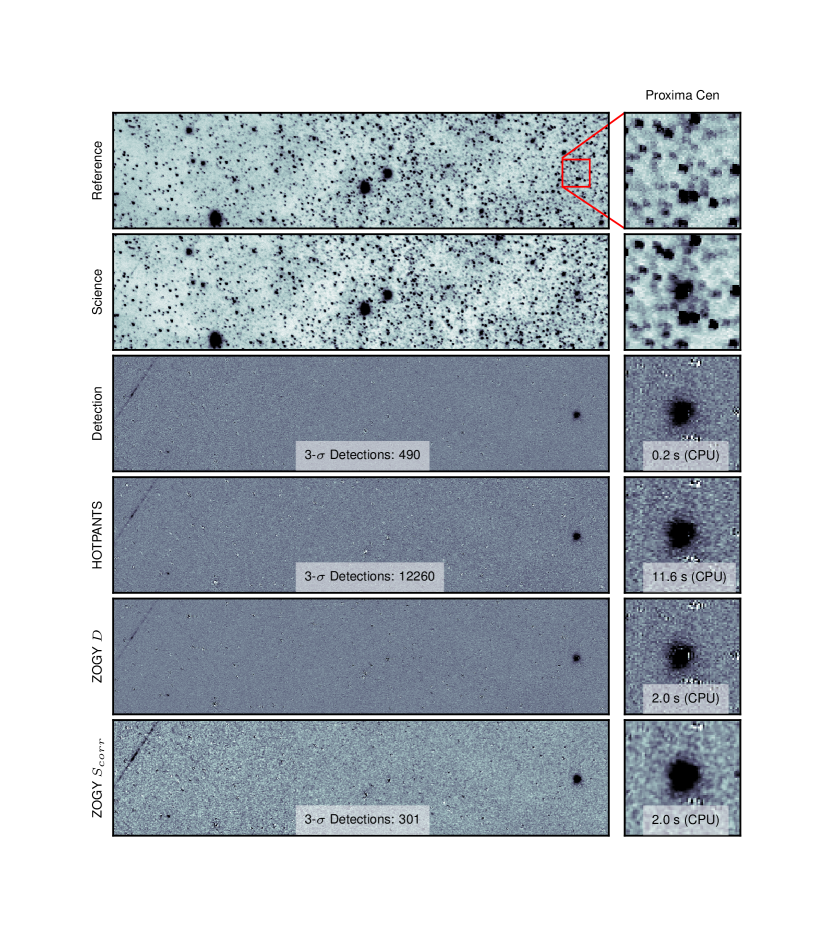
Figure 1: (Left) A $4^{\circ}\times 1^{\circ}$ region near Proxima Centauri from a reference, science, and subtraction images from EFTE, the High Order Transform of PSF and Template Subtraction algorithm (HOTPANTS; Becker, 2015), and the Zackay, Ofek, and Gal-Yam algorithm (ZOGY; Zackay et al., 2016). For ZOGY, we include both the scaled $S_{corr}$ image used for point source detection and the proper difference image $D$. In the subtraction images, a faint satellite streak (left), variable star (bottom left), and M-dwarf super flare (Howard et al., 2018) (far right) are successfully recovered. The EFTE direct subtraction produces 47% more 3-$\sigma$ detections than ZOGY for this field and can be computed is 10$\times$ faster for this image size. (Right) Cutouts from the left images showing the $1^{\prime}\times 1^{\prime}$ region centered on Proxima Cen.

An alternate approach to probing the dynamic sky at short timescales is to survey an extreme field of view, typically sacrificing some depth and resolution relative to conventional tiling surveys in exchange for rapid-cadence monitoring. This approach enables time-resolved detection of fast optical transients, and poses unique challenges and opportunities for real-time data reduction. Rapid localizations of transients across wide fields of view have recently been used to make spectroscopic observations of flares using the Ground-based Wide-Angle Camera system (GWAC) with latencies as low as 20 minutes (Wang et al., 2021; Xin et al., 2021).

Galactic transients at minute-to-hour timescales are plentiful, with stellar flares from M-dwarf stars making up the majority of these events (Kulkarni & Rau, 2006). Flares are caused by reconnections in the stellar magnetic field, producing radiation across the electromagnetic spectrum on timescales ranging from seconds to hours. Radiation from the largest events, so-called superflares, reach energies $\geq 10^{33}$ erg – orders of magnitude greater than the largest solar flares (Schaefer et al., 2000). Flares are responsible for much of the UV environment of rocky planets orbiting cool stars (Walkowicz et al., 2008), potentially providing the bioactive UV flux necessary for prebiotic chemistry (Ranjan et al., 2017), or even eroding Earth-like atmospheres (Segura et al., 2010; Howard et al., 2018). Spectroscopic observations taken during the initial stages of a flare can reveal temperature and emission-line evolution during their most impulsive phases, which is valuable for constraining fundamental flare physics as well as potential impacts of flare activity on exoplanet atmospheres. Such observations are crucial for assessing the habitability of Earth’s closest neighbors: the nearest exoplanet to Earth, Proxima Centauri b, is subject to frequent high-energy flare activity (Howard et al., 2018).

In addition to time-resolution constraints on survey design, searches for sub-hour transients like flares require software data pipelines capable of rapidly identifying candidates for spectroscopic followup and classification. Examples of bespoke pipelines optimized for minimal latency are presented in (Andreoni et al., 2017; Perrett et al., 2010; Cao et al., 2016; Förster et al., 2016; Kumar et al., 2015). Such pipelines are often built around difference image analysis, a method for isolating sources with variable flux by subtracting an earlier reference image of the field, complicated by the need to match the seeing-limited point spread functions (PSFs) of images from multiple epochs. Methods for subtracting images in the presence of variable PSFs include deconvolution with a matching kernel (Alard & Lupton, 1998; Bramich, 2008; Becker, 2015), which can be computationally expensive and numerically unstable, and more recently, the statistically optimal ZOGY method (Zackay et al., 2016), which requires a robust and static model of the image PSF, and the Saccadic Fast Fourier Transform sFFT method (Hu et al., 2022).

In this paper, we present the Evryscope Fast Transient Engine (EFTE), a real-time discovery pipeline for the Evryscopes. The Evryscopes are a pair of gigapixel-scale survey instruments which continuously image 38% of the celestial sphere at two-minute cadence. EFTE is optimized for sensitivity to short-duration transients, including stellar flares and flash-like optical counterparts to multi-messenger or multi-wavelength events. Using EFTE, we are able to produce transient candidates within survey cadence, with actionable alerts indexed into our database before the next image in the sequence. EFTE also provides a processing workflow for batch processing of Evryscope image data, and forms the basis for the Evryscope precision photometry pipeline, providing years-long light curves for every star brighter than $g\sim 15$.

One goal for the EFTE pipeline is to minimize the computational resources necessary for data analysis; a single co-located compute node supports each Evryscope site. Low resource requirements are particularly necessary when looking towards next-generation sky surveys, such as the Argus Optical Array (Law et al., 2021, 2022). The upcoming Argus Array Pathfinder instrument, consisting of thirty-eight 20 cm telescopes, will produce up to 180 TiB of data per night at 1-second cadence and 6 TiB of data per night at the base 30-second cadence; maximizing science returns from data-intensive systems like Argus will require time- and cost-efficient algorithms and pipelines. For Argus, all images must be reduced within the observing cadence to provide sufficiently low latency for followup and to avoid a backlog of data, which can require runaway compute resources for “catch-up.” Incoming Argus images are resampled to a pre-defined HEALPix (Górski & Hivon, 2011) grid using a custom GPU-based code. By parallelizing direct subtraction based on the EFTE algorithm, the Argus pipelines are able to reduce each image into transient candidates and compressed images in an average of of 925 ms. Corbett et al. (2022) presents a full description of the Argus Array pipelines and data reduction strategy.

The paper is organized as follows. In Section 2, we give an overview of the Evryscope instruments and survey strategy. In Section 3, we describe the EFTE pipeline and present algorithms for data analysis and transient discovery in ultra-wide field systems, including a simple image subtraction method suitable for time-sensitive searches (see Figure 1). In Section 4, we describe the selection metrics and machine learning (ML) approaches used to select candidates from the event stream. In Section 5, we characterize the photometric, astrometric, and latency performance of the pipeline, including the expected survey completeness and characterization of the convolutional neural network (CNN) used for vetting candidates. In Section 6, we summarize early science returns from the EFTE pipeline, including a characterization of the impact of satellite glints on rapid-response transient surveys and rapid-response observations of stellar flares using the Goodman High-Throughput Spectrograph on the SOAR 4.1 m telescope (Clemens et al., 2004). We summarize, consider extensibility of the EFTE pipeline to data from other surveys, and describe next steps towards producing a public event stream in Section 7.

2 Evryscope Survey Overview

2.1 Instrument Description

The Evryscopes are a pair of multiplexed wide-field survey telescopes, located at Cerro Tololo Inter-American Observatory (CTIO) in Chile and Mount Laguna Observatory (MLO) in California. Each site consists of up to twenty-seven 6.1 cm aperture camera units, arranged to observe the majority of the sky above an airmass of $\sim$2 simultaneously. Collectively, the Evryscopes have a instantaneous field of view of 16,512 sq. degrees (15,929 sq. degrees accounting for overlaps between adjacent cameras) with a resolution of 13.2 arcseconds per pixel across a 1.24 gigapixels combined image plane. The telescopes observe at a constant two-minute cadence with a 97% duty cycle, and collect an average of 600 GiB of data per night. While the primary Evryscope survey has been conducted in the Sloan $g$-band, the Northern Hemisphere system is also equipped with a Sloan $r$ filter for use in future surveys. All of the telescopes at each site are attached on a single mount, tracking the sky in two-hour increments.

The instruments are fully robotic, operating autonomously based on a local weather station. Evryscope-South has been in operation since May 2015, and Evryscope-North began science operations in January 2019. For a full description of the instrument and Evryscope science programs, see Ratzloff et al. (2019) and Law et al. (2015). The instrument parameters are summarized in Table 1.

Table 1: System properties for the Evryscopes. For further information, see Ratzloff et al. (2019)

Property	Evryscope-South	Evryscope-North
Field of View (Deduplicated)	8520 sq. deg	7409 sq. deg
Field of View (Total)	8832 sq. deg	7680 sq. deg
Detector Size	662.4 MPix	576 MPix
Cadence	2 minutes
Aperture	6.1 cm
Pixel Scale	13.2 arcsec/pixel
Data Rate	165 Mbps (1.2 GiB/minute)

2.2 Evryscope Observation Strategy

The Evryscopes utilize two distinct strategies for determining the two-hour-observing fields that are observed over the course of the night:

1. Semi-random, with the eastern-most edge of the field placed 30 degrees above the horizon to the east at the start of each 2-hour observation.

2. Fixed pointings, chosen from 48 overlapping regions, separated by 7.5 degrees in right ascension.

In both scenarios, the duration of a single pointing is limited by the time it takes the westward edge of the field to pass beneath an airmass of $\sim$2. This timescale (a “ratchet”) is typically on the order of two hours. Each Evryscope tracks continuously at the sidereal rate. Minimal (few arcminute) drift due to polar alignment is present over the course of a ratchet, but the visible field between consecutive two-minute exposures is consistent, point-like, and unstreaked.

Semi-random pointings (currently used for Evryscope-South) are preferred for long-term photometric performance, as diverse field positions allow sensor-plane effects to average out over the duration of the survey. Because of the commercial-off-the-shelf optics used, individual cameras exhibit up to 50% vignetting at the edge of the sensor field of view. Randomized pointings also minimize the effects of camera-to-camera periodic noise, provide some resilience against CCD sensor defects, and limit the prevalence of pathological coordinates that are always located at the edge of a sensor and thus unduly affected by optical vignetting. The trade-off is that individual fields repeat only on timescales of months (cross camera) or years (single camera), and only to few-degree precision.

Fixed-fields, by contrast, are used for Evryscope-North, and result in a fields that repeat with arc-minute precision on 1-3 day timescales. This repeatability is convenient for transient searches, as it allows us to build up an archive of reference frames to use for image subtraction. For fields above an airmass of 2, 76% are observed within two days of the previous visit, and 97% are observed within a week. Because adjacent fields overlap by $\sim 95\%$, a given sky region will appear in many different pointings, meaning that the field recurrence time is independent of the observing cadence.

3 The Evryscope Fast Transient Engine

The Evryscope Fast Transient Engine (EFTE) is a pipeline for searching Evryscope images for bright and rapidly changing sources in real-time, identifying and recording candidates across the full Evryscope FOV within the two-minute observing cadence. The primary goal of EFTE is to provide a reliable event stream with sufficiently minimal latency to enable multi-wavelength followup of events with sub-hour durations. EFTE also provides useful general-purpose utilities for interacting with and analyzing Evryscope data, including a quick-look photometry pipeline independent of the general-purpose precision-photometry pipeline, a custom astrometric solver, and CCD calibration functions. EFTE is mostly written in Python, with some compute-intensive routines (stamp extraction and photometry) implemented in C and wrapped as Python extensions using Cython (Behnel et al., 2011).

EFTE is a hierarchical + distributed system, with two analysis servers on-site at MLO and CTIO streaming reduced data products back to a central PostgreSQL relational database on campus at University of North Carolina at Chapel Hill (UNC-CH). The analysis servers each have dual AMD EPYC processors (36 CPU cores for Evryscope-North, 48 for Evryscope-South), and 512 GiB of RAM (384 GiB at Evryscope-North). The asymmetry between the two sites is due to the additional four years of archival data from Evryscope-South. The central database for reduced data products is hosted on a 36-core server with 24 TiB of flash storage, located on-campus at UNC-CH. This server also hosts a backend application for pipeline monitoring, associating EFTE transients with external alerts, and end-user reporting via a Slack-based web-interface.

In real-time operation, EFTE instances on each analysis server communicate with the Evryscope data acquisition system via a TCP socket connection, receiving notifications for each incoming image once it has been written to a shared network filesystem. EFTE maintains a per-ratchet, in-memory database of recent images to be matched for image subtraction, spawning subprocesses for all analysis tasks. Figure 2 shows the primary components of the EFTE pipeline, from the moment that an image is written to disk to reporting candidates.

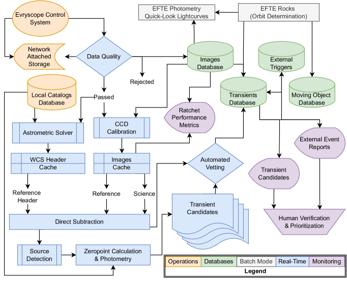
Figure 2: Data flow and layout of the EFTE pipelines. Operations (orange), and real-time reduction (blue) components are independent for each observatory, while pipeline monitoring (purple) and shared databases (green) collate data from both Evryscope-North and Evryscope-South.

3.1 Image Quality Monitor and CCD Calibration

Once an exposure is completed, the Evryscope observation daemon sends a TCP packet to an EFTE instance running on the analysis server. Upon receipt of this notification, EFTE will asynchronously record basic metadata including camera, timing, origin, and instrument configuration to the central database located at UNC-CH. Before further reduction, the image goes through a series of general quality assurance steps, including:

• verification of the file against the checksum recorded by the acquisition system

• instrument configuration checks for camera cooling, dome status, and exposure type

• autocorrelation-based checks for tracking errors and alignment failures

• sky-background measurement for saturation and linearity checks.

If these conditions are satisfied (as they are for 98% of images), the image is converted from ADU to electron units and matched to dark and flat fields for CCD calibration.

Dark frames are regularly regenerated using frames taken at the beginning and ending of each night. Cameras are cooled to a constant $-20^{\circ}C$ during observing, but some few-percent level drift in bias level is observed as a function of the camera external temperature. We believe that this is caused by temperature gradients across the readout electronics, and make a quadratic correction to the bias level as a function of the camera electronics temperature, as measured by an on-board sensor in each camera. Additionally, a small ($<1\%$) linearity correction is applied per pixel based on a cubic fit to pixel value vs. exposure time in lab testing. The linearity correction was determined to be near-identical for all our sensors.

Because of the extreme single-camera field of view, twilight flats contain significant sky gradient that the Evryscope is unable to compensate for through diverse pointings because of its fixed camera positions. Instead, we use photometric flats, calculated based on a 7th order polynomial fit to the normalized flux offsets of reference stars relative to g-band catalog photometry from the ATLAS All-Sky Stellar Reference Catalog (ATLAS-REFCAT2; Tonry et al., 2018). These frames capture the average vignetting patterns of the individual cameras, which can change sharply at the edge of the field. Photometric flat fields are stable at the 1% level over months-long timescales due to focus stability of the Evryscope Robotilter alignment system (Ratzloff et al., 2020), and are regenerated only when the instruments are cleaned, which typically requires replacing or removing the outer optical windows on each camera.

Bad pixels are replaced with the median of the surrounding $3\times 3$ pixel block and then assigned an arbitrarily high uncertainty in the resulting noise image used for photometry and source detection. Parts of each camera’s field of view, particularly those near the center of the frame, will have undersampled PSFs. Simple bad-pixel masking (i.e., assigning pixels a NaN or 0 value) will produce sharp artifacts in subsequent analysis requiring pixel resampling, like the image subtraction described in Section 3.3.

3.2 Astrometric Solutions

In parallel with the science-frame calibration steps, the EFTE pipeline produces an astrometric solution for the image using a custom solver developed for the highly distorted Evryscope focal plane. Evryscope astrometric solutions begin with an initial solve based on the center 512$\times$512 pixel region using a local install of astrometry.net (Lang et al., 2010). This solution is only used to locate the center of the image. Sources in the image are then cross-matched against the Tycho-2 catalog (Høg et al., 2000), and the offsets are used to optimize a polynomial distortion solution to 5th order in each of $x,y$ and radial position on the sensor, plus cross terms. The solution is then verified against a subset of bright stars from Gaia DR2 (Gaia Collaboration et al., 2018) based on crossmatch performance against detections in an even grid of 15 different sensor regions using the following requirements:

1. $>$ 80% recovery in at least 7 regions

2. $<$ 50% recovery in 0 regions

3. Uncertain recovery (due to source confusion or non-detections) in no more than 2 regions.

We selected Gaia DR2 for solution verification due to its reference epoch (J2015.5) coinciding with the beginning of Evryscope observations. Typical RMS offsets from Gaia DR2 positions are $\sim 4$ arcseconds, or 0.3 pixels.

The complete solution is written into a world coordinate system (WCS) header using the TPV convention for distortion polynomials (Calabretta et al., 2004). The TPV representation is an extension to the standard TAN projection, including additional terms for a general polynomial correction. Due to atmospheric refraction and tracking errors, the solution must be recalculated per-image, but the solver is able to start with a pre-computed baseline distortion solution, averaged over dozens of fields for each camera. We found that starting with an averaged solution decreased the time required for the final optimization by a factor of several on average.

This header is archived to network storage, and serialized and passed back into the in-memory EFTE matching database, where it is associated with the camera and active field. Finally, a footprint of the image, discretized as a GeoJSON (Butler et al., 2016) polygon, is stored in the central database, where it is indexed using PostGIS extension to PostgreSQL, which provides a variety of spatial object types. These footprints support a variety of use-cases, and allow users to easily query for images containing a given target, or search for images intersecting with arbitrary sky regions that can be represented as polygons, such as probability skymaps for gravitational wave and GRB triggers.

3.3 Direct Image Subtraction

Like most optical transient surveys, EFTE isolates objects with changing flux by subtracting each science image from an earlier reference frame of the same field from each image. We optimize our subtraction algorithm for speed rather than statistical optimality, electing for per-pixel operations requiring no additional intermediate data products beyond those produced in the initial photometric pipeline. Due to the short (sub-hour) timescales of interest and the dominance of instrumental optical effects on the system PSF, Evryscope images do not require PSF-matching techniques addressed by standard difference-image analysis routines, like HOTPANTS (Becker, 2015) or ZOGY (Zackay et al., 2016). However, EFTE was built for extensibility, and implementations of both HOTPANTS and ZOGY are included in EFTE.

The resolution of Evryscope images is limited by the optical distortions from the camera lenses and pixel scale, rather than atmospheric effects, under most practical observing conditions. PSFs vary greatly across the image plane of each camera, as illustrated in Figure 3; however, Evryscope image quality metrics have been measured to be stable at the few-percent level over many-month timescales (Ratzloff et al., 2020), creating highly repeatable PSFs for each individual camera.

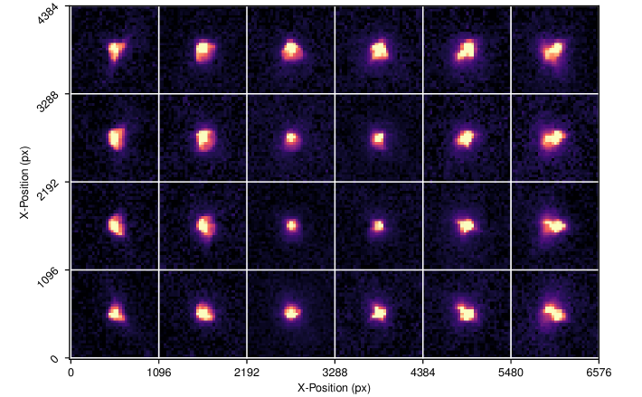
Figure 3: Median PSFs across a $6\times 4$ grid of sensor regions. PSF variability as a function of chip position is evident; however, long-term measurements of Evryscope optical stability (Ratzloff et al., 2020) indicate that the PSF is repeatable in time despite aberrations.

As a result, we adopt a straightforward algorithm for image subtraction in which the reference and science images are aligned, matched in flux, and subtracted directly. The difference of the two images is then weighted by a propagated uncertainty image to identify significant changes in flux. This approach is valid only if the following conditions are satisfied for the reference and science image couplet:

• Observed PSFs are dominated by telescope optics and pixel scale, and do not vary significantly as a function of observing conditions on the timescale of the lag between the images

• All sources have near-identical pixel coordinates in both images, offset by no more than the PSF-coherence scale, which we define as the pixel distance over which spatial PSF variation is less than thermal and atmospheric effects over a few-minute baseline, or to a 1% maximum change in the normalized PSF. This scale is typically $\sim 10$ arcminutes, or $\sim 50$ pixels at Evryscope pixel scale

• The global flux scaling between the two images is smooth

In the following subsections, we describe the process by which we match image couplets for subtraction, and the custom method we use to subtract the images that is optimized for the unique resolution and time domain covered by EFTE.

3.3.1 Reference and Science Image Selection

The primary science targets for the EFTE survey are stellar flares, which have characteristic optical rise-times of minutes. As a result, there is minimal benefit from producing reference frames widely spaced in time from our science images to maximize sensitivity to slowly varying objects. Instead, the image-matching daemon uses a sliding reference frame, taken from the same pointing as the science image. The Evryscopes maintain a consistent pointing over the course of a ratchet, with only few-arcminute drift even at the equator, meaning that the PSF for a given star is essentially constant during each two-hour tracking period, up to resampling effects caused by its sub-pixel position in the 13.2 arcsecond pixels. Additionally, using a reference image from the same pointing means that the science and reference frames are taken under near-identical sky conditions, minimizing the amount of flux scaling necessary.

In the most aggressive case, we could simply subtract consecutive images to achieve near-ideal consistency between the new and reference frames. However, immediate re-use of science images as reference images limits the survey sensitivity to only transients with a detectable change over the two-minute image interval, making confirmation images of highly impulsive events unlikely. In practice, we enforce a short lag, $\Delta t_{D}$, between the reference and science images. $\Delta t_{D}$ is typically chosen to be 10 minutes. Over 10 minutes, field drift due to polar alignment error is consistently less than 10 arcminutes (50 pixels). PSF variability over 50 pixels typically produces sub-percent subtraction artifacts, and image registration between the two images can be done with simple transformations with minimal loss in astrometric precision (see Section 5.2).

Image re-use effects are also evident at $\Delta t_{D}=10$ minutes, but only after the potential fourth confirmation image. Figure 4 shows this image-reuse effect on a real flare seen on-sky, in which the same image is both the first science image and last reference image for the transient. While the amplitude and rise time of this event enabled multiple detections up to 8 minutes after the initial detection, events with shorter rise-times or lower amplitudes may only be detected in a single epoch.

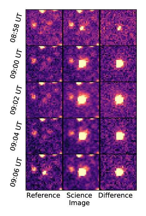
Figure 4: EVRT-192099, a 5.5 magnitude flare from a star associated with the 1RXS J174441.6-531551 in the ROSAT All-Sky Survey Bright Source Catalogue (Fresneau & Osborn, 2009; Voges et al., 1999). The reference frame from 2019 October 4 at 9:06 UT is the science image from 8:58 UT, showing the sliding reference frame used by our direct subtraction algorithm.

Additionally, the sliding reference frame causes photometry in the unscaled difference image (i.e., the numerator of equation 2) to be relative in time. Light curves of EFTE candidates are computed using forced aperture photometry in the science images, as described in Section 3.4.

Over the course of a ratchet beginning with images A, B, C, D, E and F, the pipeline will perform the following subtractions: B-A, C-A, D-A, E-A, and F-B. The rise-time sensitivity of the pipeline increases as a function of the time delay $\Delta t_{D}$ between the science image and the previous image from the same pointing chosen as a reference image. $\Delta t_{D}$ is in general a tunable parameter of the pipeline which could be increased to trade the viability of the assumptions enumerated above (and thus higher false positive/false negative alert rates) for increased sensitivity to slower rise times. Given sufficient computing, multiple instances of EFTE can run in parallel, enabling sensitivity to different science targets.

3.3.2 Image Registration

Because of the sliding reference frame selection, drift between the science and reference images amounts to a maximum of a few pixels during real-time operations that must be corrected. Additionally, small offsets can have significant effects on the sampled PSF. As such, the images must be carefully aligned and resampled to match both in position and PSF.

For the first image in a ratchet, EFTE must wait for an astrometric solution. However, the astrometric solution for subsequent images from each camera can be inferred by alignment to the first image. The effects of image registration on astrometry performance are addressed in Section 5.2. Bootstrapping the astrometric solution in this way reduces delays in the real-time subtraction process due to the astrometric solver to once per ratchet, on the first image. For image alignment and resampling, we use WCS-independent asterism-matching, using the Python AstroAlign package (Beroiz et al., 2020) to calculate a rigid transformation between the two images and perform quadratic resampling.

Alternately, in cases where a full WCS solution is available for both images (e.g., in batch reductions not conducted in real-time) the reference and science image can be aligned by resampling the images to a common grid using their WCS solutions using the Astropy-affiliated package Reproject. This has the advantage of allowing for non-rigid transformations and accounting for the effects of varying per-pixel sky area across the sensor plane. While astrometric warping due to atmospheric diffraction is negligible for typical $\Delta t_{D}$ values used for real-time reduction, WCS-based resampling is necessary for longer baselines and inter-night comparisons for fixed fields.

3.3.3 Flux Scaling

Despite the minimal baseline between the reference and science image, we fit a multiplicative flux scaling factor to the reference image to remove any discrepancies with respect to the science image due to variations in transparency and sky brightness, which is particularly important for observations during twilight conditions. Because each individual Evryscope camera covers a large sky area, we allow the flux scaling factor to vary across the image based on the results of forced aperture photometry.

First, we divide each image into $24\times 16$ 274-pixel square regions of equal pixel area, and select several thousand bright stars from the ATLAS-REFCAT2. We then calculate the sigma-clipped mean flux ratio between the science and reference images for stars in each of the 384 image sectors, and interpolate this back to full resolution using cubic splines. Finally, the flux-matched reference image $R_{m}(x,y)$ is calculated from the original, calibrated reference image $R(x,y)$ and the spatially varying flux ratio $F(x,y)$ as

$$R_{m}(x,y)=R(x,y)*F(x,y).$$ (1)

To calculate the uncertainty in the flux ratio, we calculate the standard deviation of the flux ratios for reference stars in each region and then interpolate across the full field of the image using cubic splines. The flux ratio uncertainty is propagated forward into the noise characterization for the reference image. Figure 5 shows a typical low-resolution flux ratio map for a pair of images with $\Delta t_{D}=10$ minutes, showing an average 1.7% change in transparency between the images with some internal structure. The magnitude of the scaling is consistent with transparency changes due to airmass for a camera placed at the edge of the array. Small-scale structure, when present, tends to move smoothly between images and is likely caused by high clouds.

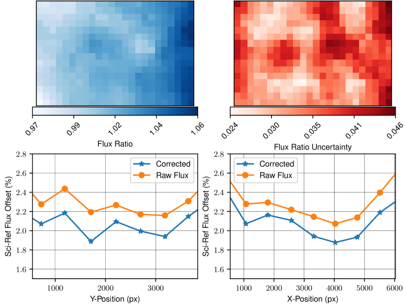
Figure 5: (Top-Left) Map of the flux ratio between a science and reference image couplet, and (Top-Right) the corresponding flux ratio error map. The flux ratio is measured based on forced aperture photometry of several thousand reference stars, and is interpolated across each full-resolution, single-camera image based on the observed flux ratio in an equally spaced grid of 384 image sectors. (Bottom) Relative aperture flux residuals before and after correcting with the interpolated flux ratio as a function of $x$- and $y$-position on the sensor. The correction improves the flux match between images by $<1\%$, which is not significant for short ($\Delta t_{D}=2$ minute) subtraction baselines. Increases in the flux offset at the edges of the image are caused by aperture losses due to the variable Evryscope PSF.

Depending on the science program, flux scaling can be skipped during reduction to minimize latency. For consecutive-image subtraction ($\Delta t_{D}=2$ minutes), we neglect flux scaling effects, as the uncertainties in the flux scaling dominate the final noise budget for the image, and the flux scaling is typically sub-percent under normal observing conditions. The primary driver of these uncertainties is likely the sub-pixel response function (sPRF), which is highly local on the Evryscope image sensors, causing the effect to not average out beyond the 1-3% level when interpolating across the image plane. Instead, multiple, slightly offset measurements of the sample star must be modeled simultaneously, as they are for the precision photometry pipeline and in coaddition of multiple images of the same field. However, we include the flux ratio for longer-baseline subtractions, where background variations can dominate over systematics.

3.3.4 Error Analysis and the Detection Image

To identify significant changes in the difference image, we need a robust accounting of the noise sources in each image. For each science and reference image, we model a spatially varying background based on sigma-clipped and interpolated mesh using sep, a Python implementation of the core routines from SExtractor (Bertin & Arnouts, 1996; Barbary, 2016). The standard deviation of the background $s_{B}$ is also measured at this step, based on the sigma-clipped standard deviation. $s_{B}$ is treated as an empirical measure of the Gaussian noise contributions to each image, including the readout noise and dark current uncertainty. We note that this approach can overestimate the noise due to Poisson contributions from unresolved background star light, and as a result, the detection significance in the direct subtraction image will tend to be an underestimate, particularly in crowded fields (e.g., near the galactic plane).

For a given combination of science image $S(x,y)$ and flux-matched reference image $R_{m}(x,y)$, both in electron units, the detection image $D(x,y)$ is defined as

$$D(x,y)=\frac{S(x,y)-R_{m}(x,y)}{\sqrt{s_{S}^{2}(x,y)+s_{R}^{2}(x,y)}},$$ (2)

where $s_{S}^{2}$ and $s_{R}^{2}$ are the total noise images for $S$ and $R_{m}$, given by

$$s_{S}(x,y)=\sqrt{S(x,y)+s_{BS}^{2}(x,y)},$$ (3)

and

$$s_{R}(x,y)=R(x,y)\sqrt{\frac{R(x,y)+s_{BR}^{2}(x,y)}{R^{2}(x,y)}+\frac{s_{F}^{2}(x,y)}{F^{2}(x,y)}},$$ (4)

where $s_{BS}(x,y)$ and $s_{BR}(x,y)$ are the measured background standard deviation maps of the science and reference images, respectively, $F(x,y)$ is the flux ratio between the two images, and $s_{F}(x,y)$ is the spatially varying uncertainty in the flux ratio. $D(x,y)$ image is the simple difference in the two images, scaled by the combined per-pixel uncertainty. The detection image has units of standard deviations. We again use sep to mask the detection image at the desired threshold and identify sources.

Figure 1 shows an example of an image couplet in a crowded field, along with the resulting direct subtraction image. We also include subtraction images produced using the HOTPANTS and ZOGY algorithms (Becker, 2015; Zackay et al., 2016). Direct subtraction produces more false positives (488) than ZOGY (299 in $S_{corr}$) at the 3-$\sigma$ threshold, but two orders of magnitude fewer than HOTPANTS (12258). While ZOGY is a computationally efficient approach, direct subtraction is faster by a factor of ten, largely due to the requirement to calculate a PSF model for ZOGY. Using the direct detection image, we successfully identify three astronomical transients with the EFTE pipeline using the vetting procedures described in Section 4.

3.4 Photometric Zeropoints and Forced Photometry

To calibrate magnitudes for EFTE transient candidates to a standard photometric system, we build a spatially varying photometric zeropoint based on a subset of the ATLAS-REFCAT2, a composite catalog consisting of $griz$ data from the AAVSO Photometric All-Sky Survey (APASS; Henden et al., 2016), Pan-STARRS Data Release 1 (Flewelling et al., 2016), Skymapper Data Release 1.1 (Wolf et al., 2018), Tycho-2 (Høg et al., 2000; Pickles & Depagne, 2010), the Yale Bright Star Catalog (Hoffleit & Jaschek, 1991), GAIA DR2 (Gaia Collaboration et al., 2018), plus original data from the ATLAS Pathfinder survey. To ensure that stars used for determining the zeropoint of the image are well-exposed, but not saturated, we select a subset of the catalog between $10<{g^{\prime}}<12$. We also exclude stars with colors redder than $g-r=1.5$ that might bias the photometry due to unconstrained chromatic aberrations affecting the PSF. We calculate an instrumental magnitude for each of the reference stars using a forced aperture at the catalog position in the background-subtracted and calibrated science image, typically with an aperture radius of 3 pixels (40 arcseconds).

To model the variation in photometric zeropoint across the field of view, the science image is divided into an $8\times 12$ grid of square subframes, each of which subtends 4 square degrees and contains O(100) reference stars. Within each subframe, we calculate the sigma-clipped median offset between the instrumental magnitudes calculated via aperture photometry and the catalog values. The offsets in each region are then smoothly interpolated over the rectangular mesh of the full-sized using quintic splines to produce a spatially varying zeropoint $z(x,y)$. The resulting image has units of magnitudes and has as its values the photometric zeropoint at each pixel, defined such that

$$m_{g}=-2.5\log_{10}{F_{aper}}-z(x,y),$$ (5)

where $F_{aper}$ is the measured flux from aperture photometry.

Finally, we calculate magnitudes for each candidate detected as described in Section 3.3.4, based on their centroid positions in the detection image. Centroids are calculated for each candidate by computing their value-weighted average position (“center of mass”). This process uses a custom aperture photometry routine, implemented in Cython for the Evryscope precision photometry pipeline (Ratzloff et al., 2019), on the science image.

4 Automated Vetting

Despite the optical consistency of Evryscope images chosen for subtraction, the direct subtraction process produces thousands of false positives per image. Observed sources of false positives are plentiful from inside the CCD sensors out to Earth orbit, including:

• Cosmic ray muon tracks

• Compton recoil electrons from radionuclides in materials at the observatory

• Optical ghosts

• Registration and astrometric errors

• Persistent residual charge from bright stars remaining after cycling the detectors

• Flat-fielding errors

• Aircraft strobes

• Tumbling satellites and debris (Corbett et al., 2020)

• Noise artifacts from both photon and astrometric noise.

In total, the event rate from these sources can outnumber the real, on-sky rate of astrophysical transients by orders of magnitude. Human candidate inspection remains standard, but it is not scalable to surveys producing hundreds of thousands of candidates per night. As a result, a reliable, efficient, and automated vetting system for candidates is a core component in any transient survey producing an actionable event stream that can be delegated to followup resources.

Some false-positive sources in the list above can be identified with simple filters: Bright streaks from satellites involve thousands of pixels, and residual charge from bright stars can be flagged based on previous astrometric solutions. Other classes of observed signals can be difficult to identify from simple metrics in all scenarios. To account for this, we use a combination of data cuts based on explicit filters and machine learning (ML) methods.

4.1 Initial Candidate Filters

While ML techniques can be comprehensive, simple filters grounded in domain knowledge can be both more efficient and more easily interpreted. Starting from an initial deep source extraction ($SNR>3$ in a minimum of 1 pixel) of the detection image $D(x,y)$, we implement three first-order quality cuts, removing candidates which meet any of the following conditions:

1. Centroid within 15 pixels of the edge of the CCD

2. Ratio of negative-to-positive pixels within a 6-pixel circular aperture $>0.4$

3. More than $750$ pixels above the detection threshold

Detections near the edge of a CCD are typically caused by small amounts of mount drift between the science and reference images. Large ratios of negative to positive pixels typically indicate a photon or astrometric noise artifact. Extended events $>750$ pixels are commonly bright streaks, caused predominantly by aircraft and LEO satellites.

We apply an additional filter after the ML vetting described below; we reject any candidates coming from a subtraction with more than 500 high-confidence candidates. These failed subtractions rarely occur, and are caused by a doubled or streaked image due to wind shake at the instrument, or a breakdown of the assumption of a slow and smoothly varying sky background required for direct image subtraction, as described in Section 3.3.

With no additional vetting, these simple filters reduce the per-image candidate count to O($10^{2}$) using the baseline values stated above; however, these numbers are readily tunable to the science case and corresponding false positive tolerance, either by modifying a configuration file for the EFTE pipeline instance running at each observatory, or by filtering the database queries used to regularly report candidates to end users. Candidates that pass the thresholds for these filters at the pipeline-instance level are inserted into the central database, including small $30\times 30$-pixel “postage stamp” cutouts around their detection positions.

4.2 vetnet: Real-Bogus Classification with Convolutional Neural Networks

For additional reduction of the EFTE false positive rate, we use an ML model based on two-dimensional convolutional layers (LeCun et al., 1989) with weights conditioned directly on image data. This model is a binary (“real/bogus” [RB]) classifier, which assigns each candidate a score between 0 and 1, where a score of 1 indicates that the candidate is likely real. RB classifiers have seen long-standing use in transient surveys, starting with the model built by (Bailey et al., 2008) for the Nearby Supernova Factory (Aldering et al., 2002). Similar approaches have been used for the Palomar Transient Factory (PTF; Law et al., 2009; Bloom et al., 2008), the Intermediate Palomar Transient Factory (iPTF; Brink et al., 2013), the Dark Energy Survey (Goldstein et al., 2015), and most recently, for ZTF (Mahabal et al., 2019; Duev et al., 2019) and GOTO (Killestein et al., 2021).

Deep learning is a type of ML in which “deep” stacks of artificial neural network layers (Mcculloch & Pitts, 1943) are used to transform input data into latent-space encodings that can be mapped to the desired output quantities. Convolutional Neural Networks (CNNs) (LeCun & Bengio, 1995) are a sub-class of artificial neural networks that build up a latent space representation of pixel data using convolutions, which identify increasingly compressed features of the input as the depth of the network increases, as opposed to requiring pre-selection of computed - and potentially sub-optimal - features to represent the data. CNNs have found widespread use in astronomy for tasks including source detection and deblending (Stoppa et al., 2022; Burke et al., 2019), in addition to transient real-bogus vetting (Makhlouf et al., 2021; Förster et al., 2016; Duev et al., 2019; Killestein et al., 2021).

In this section, we describe vetnet, a CNN-based vetting algorithm trained to assign real-bogus probabilites to EFTE candidates directly from 30$\times$30 pixel cutouts from the reference, science, and direct subtraction difference images.

4.2.1 Training Set and Data Labelling

Supervised ML classifiers require large datasets of labelled examples to identify the complex latent associations during training. In general, there are two options for producing these datasets: simulation or human classification. Exclusively training on simulated data is risky because the efficacy of the final model is dependent on how representative the simulations are of real data. However, human classification is labor-intensive, and prohibitive at the level of producing thousands or even millions of labelled examples across a representative sample of the survey.

As a result, we have adopted a compound approach, using both hand-labelled, on-sky data and simulated events produced via spatially varying PSF injection. The simulated dataset was used to train intermediate models to pre-screen events for human labelling, including the prototype CNN used in Corbett et al. (2020). We manually classified the on-sky, moderate-purity sample produced by the intermediate model to produce a smaller, but minimally contaminated and representative, data sample for training the production models.

4.2.2 Network Architecture

vetnet uses a sequential, VGGNet-like (Simonyan & Zisserman, 2014) model with six trainable layers; four convolutional, and two fully connected output layers. Each set of convolution layers is subject to 20% dropout to prevent overfitting, encouraging the model to build a diverse set of representations of the data distribution. The dropout fraction at each layer was determined using the HyperBand band algorithm (Li et al., 2018) with a binary cross-entopy loss function. Further regularization is provided by a pooling layer, which reduces the dimensionality of each convolution block output by a factor of four. Outputs of each pooled layer are normalized and re-centered on zero using batch normalization (Ioffe & Szegedy, 2015) to improve training performance and model stability. All convolution layers use 3-pixel square kernels and ReLu activation (Agarap, 2018), save for the final fully connected node, which has a sigmoid activation function that produces an output value normalized between 0 and 1. This output, the vetnet real-bogus (RB) score, can broadly be interpreted as probability that a given candidate is real. Figure 6 depicts the architecture of the model, including filter depths and the resulting dimensionality.

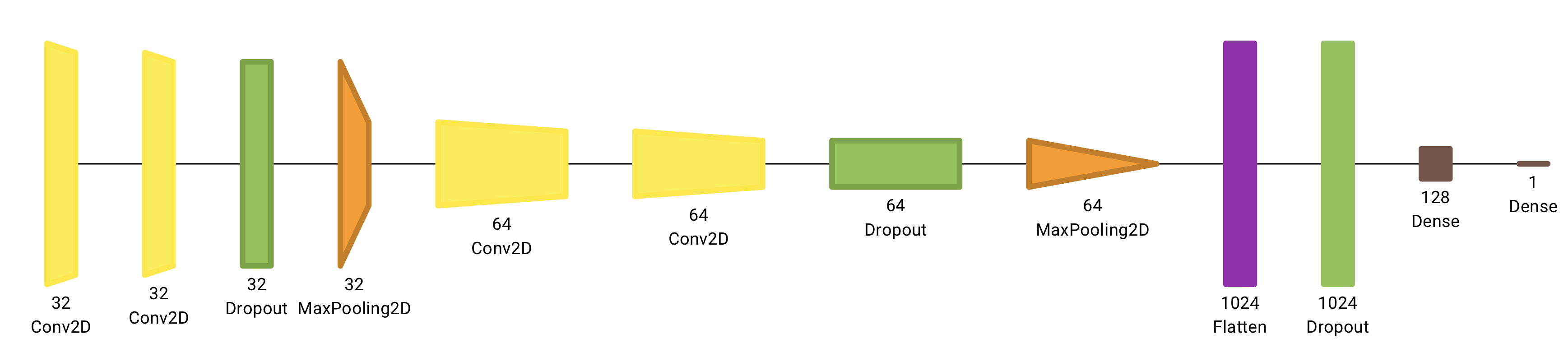
Figure 6: Architecture of vetnet, a convolutional real-bogus classifier used by EFTE. The inputs to the network are a triplet of 30$\times$30 pixel cutouts around the center of each candidate, taken from the reference, science, and direct difference images. All trainable layers, save for the final dense unit, use ReLU activation. Pairs of convolution layers are each followed by max-pooling layers and 20% dropout for regularization. Network visualization generated with Net2Vis (Bäuerle et al., 2021).

vetnet is implemented in Tensorflow (Abadi et al., 2015), using the high-level Keras API (Chollet et al., 2015).

4.2.3 Dropout and Model Uncertainty

CNNs can have an arbitrarily large number of free parameters, and are accordingly able to overfit training data. As a result, methods of regularizing the training process and the weights assigned to the convolutional filters are necessary to maximize performance on actual data at inference time. Dropout (Srivastava et al., 2014) is one common technique, in which a tunable fraction of outputs from a layer are chosen at random and set to zero, preventing them from contributing to the final network outputs.

In addition to slowing overfitting, dropout also can be interpreted as an approximation of Bayesian inference (Gal & Ghahramani, 2015a). In this framework, each random sampling of layer outputs can also be considered a sample from the distribution representing network weights in a fully Bayesian network. Evaluating a given sample through these different dropout-induced realizations of the network enables us to similarly approximate the posterior distribution of the network output. The advantage of this approach, called Monte Carlo (MC) Dropout, is that the output distribution includes the systematic uncertainty in the network output due to model selection, distinct from the random uncertainty produced by the variance of the training set (Gal & Ghahramani, 2015b). To produce an output from the network, each candidate is processed through multiple dropout-induced realizations of the network, producing a distribution of resulting RB scores. We use the median of this distribution as the RB probability for each source.

Interpretation of MC Dropout is unsettled in the literature (namely, whether it represents a genuinely Bayesian approximation (Le Folgoc et al., 2021)). However, it can be used to produce a number that scales with the degree of consensus within the network and amount of support for a sample within the training set, and that can be interpreted as a confidence metric. This is similar to the interpretation of the sigmoid activation of the network as a whole as a real-bogus probability, despite not representing a normalized probability density function. We adopt the entropy-based metric from Killestein et al. (2021) to quantify the network confidence:

$$\mathbb{C}=\frac{1}{N}\sum_{i=1}^{N}-p_{i}\log_{2}{p_{i}}-(1-p_{i})\log_{2}{(1-p_{i})},$$ (6)

where $N$ is the number of samples from the posterior distribution and $p_{i}$ is the network output for the $i$th sample. The metric $\mathbb{C}$ is the binary entropy of the Bernoulli process representing real-bogus classification, averaged across posterior draws, and is bounded on the interval $[0,1]$. In Section 5.3, we demonstrate that $\mathbb{C}$ also matches the subjective confidence of human vetting.

The number of forward passes used to approximate the network output posterior distribution is determined empirically from the validation set. Figure 7 shows the accuracy of the classifier as a function of the number of forward passes through the network. The accuracy of the median RB score converges after 10 inferences, which is consistent with the findings in Killestein et al. (2021), despite the dropout rate here being two orders of magnitude higher.

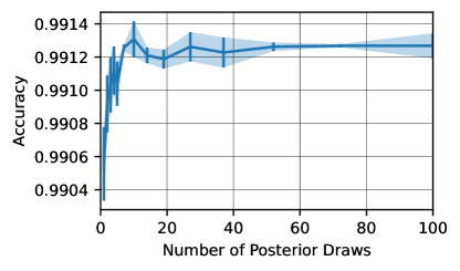
Figure 7: Network accuracy vs. number of forward passes through the network for the validation set. Performance converges at 10 samples. Error bars represent the standard deviation of the results across 20 iterations.

4.2.4 Training Set and Data Augmentation

Two datasets were used to train the vetnet classifier; the 435,452 simulated candidate dataset described in Section 4.2.5, and a human-annotated sample of on-sky detections containing 31,092 candidates flagged as probably real by an earlier iteration of vetnet itself (Corbett et al., 2020). Unlike the simulated dataset, the on-sky data is heavily class-imbalanced, with only 9.6% of examples (2,976) being human-labelled as real. To account for this class imbalance, we randomly exclude 25,140 of the bogus samples from the on-sky dataset, noting that the simulated dataset only contains simulated examples of the real class. Bogus examples within the simulated data set are drawn from the same population as the bogus examples in the on-sky dataset. Our approach for maximizing the return from this relatively small sample of on-sky data is described in Section 4.2.6.

We divided the simulated and annotated on-sky datasets into training, validation, and testing subsets using an 80:10:10 ratio. We used validation set for tuning the MC Dropout fractions and the number of posterior draws, and for monitoring the training process.

To extend the effective size of the dataset, random flips and rotations are applied to each batch of training samples. As noted by Killestein et al. (2021) and Dieleman et al. (2015), rotations (other than in 90 degree increments) require interpolation and thus distort the data from the pixel grid; however, in our use case, the data are previously resampled with interpolation by the image alignment process (see Section 13). No data augmentation is applied during validation or model evaluation, or for training during fine-tuning with human-annotated data.

4.2.5 Simulated Data Generation

We generated a base training set by injecting simulated transients into 300 randomly selected images across the first two years of full Evryscope science operation at each site. Images were selected uniformly in time, meaning that moon phase, sky conditions, focus changes due to temperature variations, and dust-accumulation on the instrument (leading to measurable changes in the background level and limiting magnitude on few-month timescales) are uniformly represented. Each image was calibrated as in the pipeline (see Section 3.3).

For each image, we generated a uniform sample of 5,000 positions within the image, then deduplicated so that no position was within 50 pixels of any other position to avoid overlapping transients, resulting in an average of 1,200 injections per image. While this does bias the initial training set against contemporaneous, spatially coincident events, this is sufficiently rare that we neglect this scenario. Each injection was assigned a random magnitude, drawn from a uniform distribution bounded between the typical saturation limit of g$\sim 7$ and the 1.5$\sigma$ detection limit at the injection position (determined by the photometric zeropoint interpolation procedure described in Section 3.4).

A second round of injections was done to simulate transients with known visible progenitors. From the catalog stars within each image, 500 stars minimally separated by 50 pixels were selected as additional positions for injection. The variability amplitude was uniformly sampled between 0.25 and 8 magnitudes. The upper limit is set by the maximum contrast visible for a pre-detected star in an Evryscope image, i.e., a star at the dim-limit of the survey that reaches the single-exposure saturation limit.

Evryscope PSFs are heavily impacted by optical aberrations, and exhibit a wide variety of morphologies, both between cameras and across the field of view of individual cameras (Ratzloff et al., 2020), making common analytic profiles (Moffat, Gaussian, Lorentzian) untenable. Further, the coarse pixel scale makes more complex linear models, such as the ePSF (Anderson & King, 2000) and those used by PSFEx (Bertin, 2011) and PSFMachine (Hedges et al., 2021), prone to poor fits due to aliasing and source confusion. We found that the most robust method for simulating transients with morphologically plausible, point-like profiles was to build a model PSF based on nearby, isolated stars. For each injection position, up to 100 nearby stars having a distance less than 137 pixels and significance of 10$\sigma$ above the local noise are extracted with a 30$\times$30 “postage stamp” window. Each stamp is then multiplied by a smoothly varying (Hanning) window and normalized. The final PSF to be flux scaled and added into the image is the median of the nearby stamp templates, weighted by the relative normalized distance from the injection position and relative flux uncertainty of the template star. Figure 8 shows examples of simulated PSFs using this technique across a typical Evryscope focal plane for a range of magnitudes, alongside the resulting signal in a direct subtraction image with a consecutive epoch.

At the end of the transient injection process, the image is “de-calibrated” by adding back in the expected dark current, bias, and background levels, and the image is converted back into ADU units with pixel values beyond the range of an unsigned 16-bit integer truncated, matching the histogram of the simulated images to the distribution expected for science images.

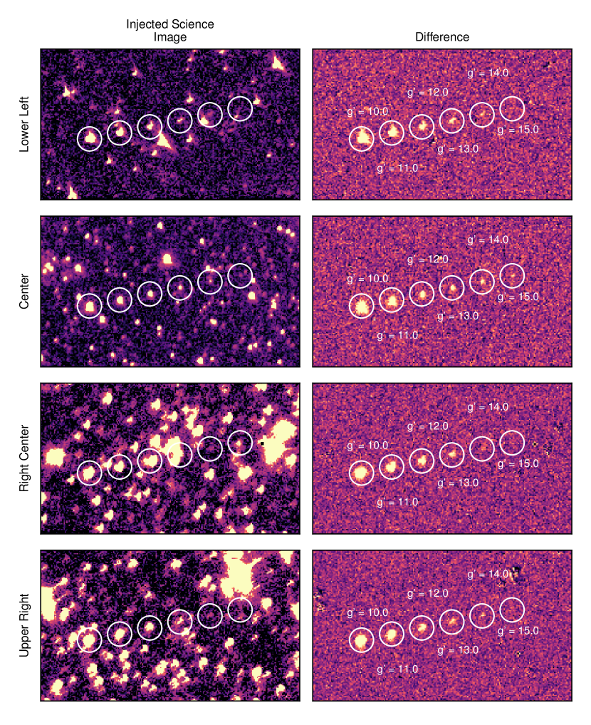
Figure 8: (Left) Examples of simulated transients with magnitudes $g^{\prime}=10,11,12,13,14,15$ at the center and edges of a typical mid-galactic latitude Evryscope image. PSFs at each position are modeled as a normalized, aligned, and sigma-clipped combination of nearby isolated stars, producing morphologically plausible, star-like injections. These simulations are used for initial conditioning of our machine-learned vetting system. (Right) Difference images for each subimage using a reference frame taken two minutes before the injected science image.

To produce a simulation-augmented dataset, the transient-injected images are reduced using the EFTE pipeline, and any candidates identified within 2 pixels of an injection location are labelled as real, and all others as bogus. Despite the large number of injected sources, this process produces an unbalanced dataset, with artifact detections outnumbering injections at rates up to 1000-to-1. To balance the dataset, we randomly select a number of bogus candidates equal to the number of recovered injections for inclusion in the final data set. This results in a dataset with noisy labels due to both background transients (likely dominated by short-duration reflections from Earth satellites (Corbett et al., 2020; Nir et al., 2020)) and candidates injected below the difference image threshold and recovered coincidentally. From visual inspection of 10,000 injection candidates, uniformly sampled from both known-injections and predicted artifacts, we estimate label contamination to affect $\leq 2.7\%$ of the candidates in the 435,452 candidate dataset. Deep convolutional models have been observed in prior work to be robust to many times this level of label noise (Ghosh et al., 2016; Rolnick et al., 2017).

4.2.6 Staged Training Methodology

A common approach for building specialized models with limited training data is to utilize transfer learning, leveraging the pre-trained feature representations of existing models built with massive related datasets. Rather than training an entire model from scratch, which requires a large annotated dataset over the domain of interest, a pre-trained model can be selectively “fine-tuned” over a representative dataset in a new domain. We adopt a similar approach for making use of the considerable diversity of observing conditions and sky regions represented in the simulated dataset described in Section 4.2.4, while minimizing the risk of optimizing for properties of the transient injection process (see Section 4.2.5) rather than properties transferable to on-sky data.

Our training curriculum for vetnet was as follows:

1. Train the full model, including all convolutional and fully connected layers, on the simulated dataset until convergence to create the synthetic base model

2. Freeze the weights on all convolution layers from the synthetic base, and re-train the fully connected layers from scratch using on-sky data

3. Unfreeze the convolution layers, train at a minimal learning rate using on-sky data until convergence to produce the final on-sky model.

We used the Adam optimizer (Kingma & Ba, 2014) with a binary cross-entropy loss function for all three stages. For the first two training stages, we start with a maximum learning rate of 0.0003, slowed by a factor of two whenever the loss on the validation set plateaued for 10 epochs. Scheduling the learning rate in this way helps the network to converge to a local minimum when near a global minimum and decreases the oscillation around the minimum of the loss function. For the final fine-tuning of the entire model, we reduced the initial learning rate to 0.00001 while maintaining the same scheduled rate decay.

The synthetic base model converges after $\sim$100 epochs, taking about 6.5 hours when training on an Intel Xeon E5-2695v4 CPU. Fine-tuning with on-sky data converges after $\sim$150 epochs, but takes less than 10 minutes due to the smaller quantity of data.

In the final stage, we use a single-iteration of the semi-supervised relabelling routine suggested by Killestein et al. (2021); samples in the training set which are classified differently by the network than by human labelers are flipped to the model classification in cases where the model confidence $\mathbb{C}$ is greater than the median. On review, these samples are generally either difficult to classify by hand, with low-significance peaks relative to the surrounding noise, areas of the sensor plane with pathological PSFs, or likely errors in the original labelling process. Figure 9 shows three representative examples that are re-labelled by vetnet during this process. In total, less than 4.7% of samples are changed in the training set after updating the labels. We note that this is comparable to the label noise in the synthetic dataset (2.7%).

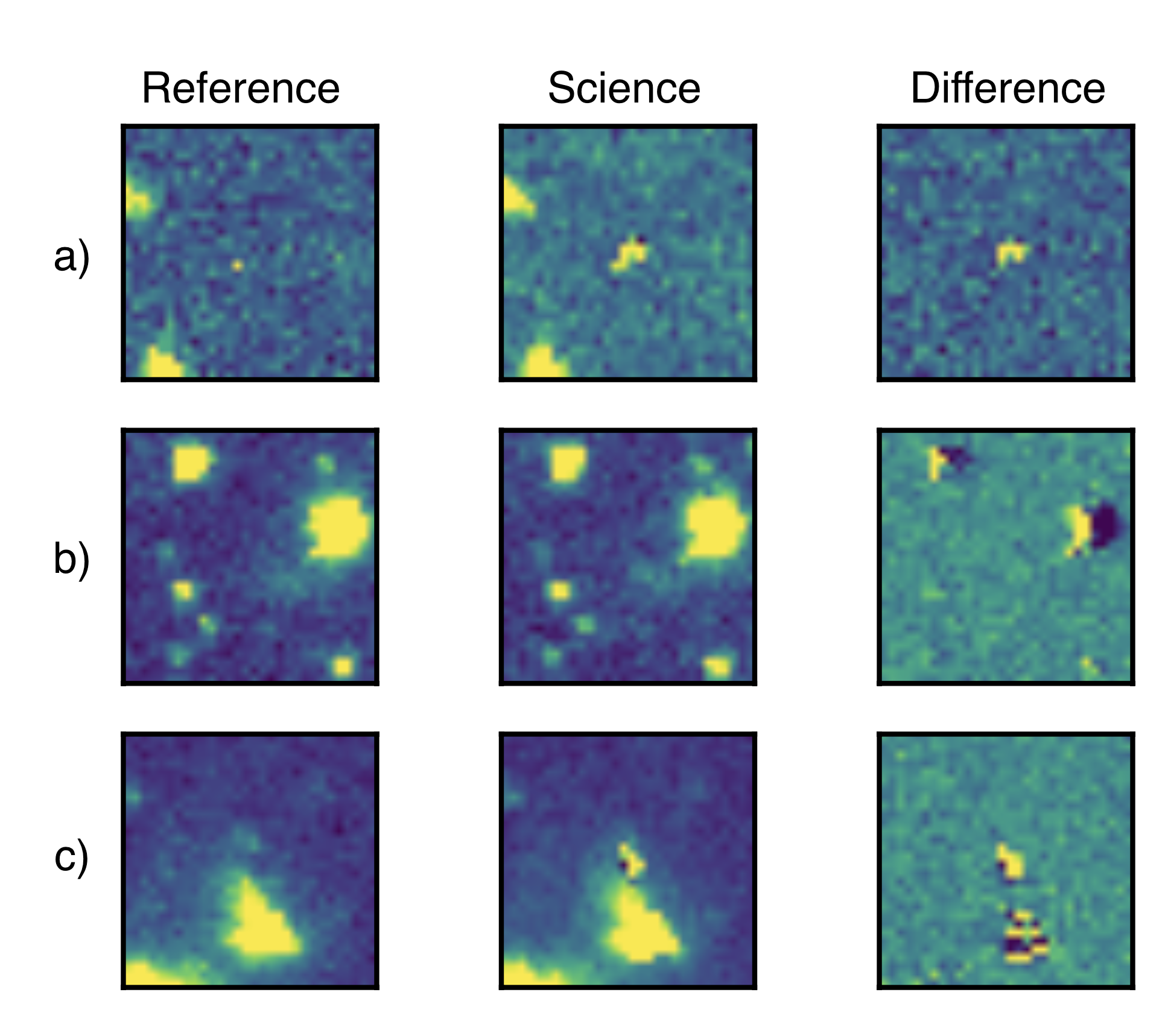
Figure 9: Misclassified training set samples re-labelled based on the entropy-based confidence of vetnet predictions. Network reclassifications typically affect samples which are difficult to classify manually. Samples (a) and (c) were initially classified as real by human vetters, but were relabeled as bogus by the algorithm. Both have pathological PSFs likely caused by interpolation artifacts from resampling near a cosmic ray, particle strike, or unmasked bad pixel. Sample (b) is low-significance and off-center, but was manually classified as bogus before being confidently relabelled as real by vetnet.

4.3 Candidate Crossmatching and Source Association

EFTE candidates from both sites and their corresponding metadata are stored in a relational database. On insert, candidates are associated with previous candidates at the same position, which collectively form an “event,” via an insert trigger within the database. If a candidate has no antecedent, a new event is created, and an additional trigger crossmatches the new event’s position with a variety of externally produced reference catalogs. At time of writing, these reference catalogs include the International Variable Star Index (VSX; Watson et al., 2020), the Galaxy List for the Advanced Detector Era (GLADE; Dálya et al., 2018), ATLAS-REFCAT2, and the ASAS-SN Catalog of Variable Stars (Jayasinghe et al., 2018). Stellar sources are crossmatched with a radius of 26 arcseconds (corresponding to 2 Evryscope pixels and the worst-case astrometric performance for EFTE detections - see Figure 13), and galactic sources from GLADE are crossmatched with a 1 arcminute radius.

To accelerate the in-database crossmatching and candidate queries, all candidates, events, and reference catalogs are indexed using the Quad Tree Cube (Q3C) pixelization scheme, a PostgreSQL extension for efficient spherical crossmatching and radial queries (Koposov & Bartunov, 2006). Sky areas, such as the on-sky footprints of images or probability contour regions for multi-messenger transient events, are indexed using PostGIS with a custom non-geodetic projection. This projection does not include the WGS-84 (Kumar, 1988) reference ellipsoid, and represents the right ascension and declination in the standard barycentric celestial reference system in all EFTE application code.

Candidates can also be crossmatched against external triggers received by EFTE via automated circulars from the NASA Gamma-ray Coordinates Network/Transient Astronomy Network (GCN). Alerts are inserted in the central database by an automated ingest microservice, where they are indexed by position either using Q3C for tightly localized triggers, or as PostGIS polygons for events that are distributed as polygon skymaps, like LIGO/Virgo skymaps (Abbott et al., 2009) or GRB alerts from the Fermi Gamma Burst Monitor (Fermi GBM; Bhat et al., 2009).

5 Pipeline Performance Evaluation

5.1 Photometric Solutions

To evaluate the performance of the photometric calibration using a smoothly varying zeropoint, as described in Section 3.4, we compare single-epoch forced photometry from 3,217,215 catalog stars from the ATLAS-REFCAT2 across 500 randomly selected images from the 2018 observation year. The images were required to pass the quality assurance metrics described in Section 3.1, but were not otherwise filtered for sky or instrumental conditions. Figure 10 gives the distribution of photometric offsets and offset RMS as a function of magnitude in individual images. The resulting photometry is calibrated to the reference catalog with an RMS offset of 0.05 magnitude between $8<m_{g}<14.0$, measured using 5 iterations of a 5-$\sigma$ clip to remove outliers due to single-epoch failures.

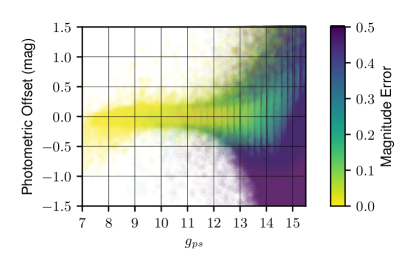
Figure 10: Photometric calibration offsets between the ATLAS All-Sky Photometric Reference Catalog and EFTE. Median RMS offset in the region $8<m_{g}<14.5$ is 0.06 magnitude. Anomalously bright and high-precision measurements (upper right) are due to source confusion and blending. Under-reporting of magnitudes due to saturation is evident for stars brighter than $g^{\prime}=8$.

These numbers likely represent an upper limit on photometric RMS for isolated and dim events, as the distribution is dominated by source confusion beyond $g^{\prime}=14$ (e.g., dim catalog stars with a brighter star near or within the 6-pixel aperture), causing anomalously bright and high-precision measurements of dim catalog sources. Sources brighter than $g^{\prime}=9$ are occasionally saturated when they appear near the center of the image, though typically, sources as bright as $g^{\prime}=8$ are well-calibrated and linear. There is a noise floor around $\sim 5\%$ for single-epoch detections from Evryscope due to variation in the sub-pixel response across the image plane. These effects are modeled in data products from the Evryscope precision photometry pipeline (Ratzloff et al., 2019), but are prominent in raw single-epoch bright-star photometry from EFTE.

Additional color and airmass terms can be applied to light curves of EFTE photometry as needed, using the equation

$$g_{EVR}=g_{PS}+A+B(g_{PS}-r_{PS})+k_{1}X+k_{2}X(g_{PS}-r_{PS}),$$ (7)

where $g_{EVR}$ is the magnitude in Evryscope $g$-band, $g_{PS}$ and $r_{PS}$ are the PanSTARRS magnitudes from the ATLAS reference catalog, $X$ is the airmass of the star, and $A$, $B$, $k_{1}$, $k_{2}$ are fitted photometric conversion factors between the Evryscope and PanSTARRS bandpasses. Based on fits to forced-aperture light curves using a robust estimator (Fischler & Bolles, 1981), the photometric conversion terms are $A=0.037\pm 0.002$, $B=-0.051\pm 0.004$, $k_{1}=0.021\pm 0.002$, and $k_{2}=-0.051\pm 0.003$. The light curves used to fit these parameters were chosen from a random sample of 25,000 Northern Hemisphere stars, which we then filtered based on a quality metric which includes source variability relative to nearby stars, saturation, and the shape of the aperture flux growth curve, leaving a cleaner sample of 10,671 lightcurves with an average of 17,140 epochs.

Figure 11 shows the photometric offset as a function of $g-r$ and $g-i$ colors before and after applying the calibration offset, as well as the resulting impact on the long-term photometric accuracy of light curves. Application of the color and airmass correction brings the RMS calibration accuracy of long-term light curves from 0.16 mags to 0.06 mags, in line with the single-epoch measurements above.

Figure 11: (a), (b) Photometric offsets between Evryscope and PanSTARRS g-band as a function of $g-r$ before and after calibration with the color and airmass terms above, respectively. Large offsets below the linear trend are caused by blended sources and low-SNR detections that were not filtered based on the light curve quality metric described in Section 5.1. (c), (d) Same as above, but with $g-i$ colors in place of $g-r$ to demonstrate perfomance over a wider variety of colors. No calibration fits are made as a function of $i$-band colors. (e), (f) Photometric calibration performance for many-epoch light curves as a function of magnitude. The sigma-clipped RMS photometric offset decreases from 0.16 mags to 0.06 mags for sources between $8<m_{g}<14.5$ with application of color terms.

Public EFTE data products, including both transient alerts and long-term photometric light curves , do not include color and airmass terms. For light curves , calibration for photometric precision, rather than accuracy, is prioritized. Evryscope light curves are first decorrelated from subpixel PSF variations, and then detrended using a customized version of the SysREM algorithm (Tamuz et al., 2005) to correct for systematics, ultimately producing light curves that are self-consistent at the $\leq$20 mmag level at the bright end of Evryscope’s operating range, as shown in Figure 12.

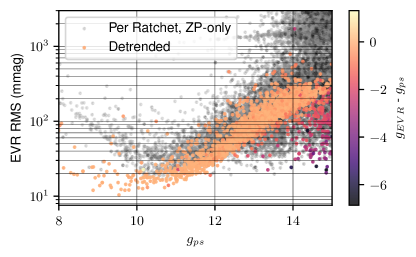
Figure 12: Measured RMS of 10671 randomly selected, long-term Evryscope light curves. Performance in the detrended lightcurves ranges from 20 mmag at the bright end to 20% for dim sources. RMS for raw light curves is an average of the measured RMS in each pointing, neglecting zerpoint offsets between ratchets.

5.2 Astrometric Localization

The custom astrometry routines developed for the Evryscopes are capable of providing 1-2″(0.08-0.15 pixel) RMS astrometry over the field of view of the Evryscopes in single images; however, astrometric localizations from EFTE also depend on the quality of the alignment procedure used for real-time reduction, and must therefore be characterized separately. In addition to the sub-pixel scatter induced by photon noise, EFTE localizations depend on the consistency of the pointing between consecutive images and the accuracy of the rigid transformation calculated to align each image with the previous image for which a WCS solution is available.

We evaluated the quality of this alignment routine by performing source detection in individual science images aligned to a previous target image in the same pointing. We chose target images with a typical $\Delta t_{D}$ of $10$ minutes, with samples of $\Delta t_{D}<10$ minutes representative of what would occur in the first few images in a ratchet.

The detected sources were then cross-matched with sources in the ATLAS-REFCAT2 (Tonry et al., 2018). As in Section 5.1, 500 science images for testing were randomly selected from the 2018 observing data set, across all weather and Moon conditions. Figure 13 shows a histogram of the offsets between the catalog positions and the recovered positions in the aligned science image with a re-used WCS solution. Astrometric performance was sub-pixel for 99% of detected sources, with an RMS scatter less than 4 arcseconds between 8th and 14th magnitude. As for the photometry, precision is limited by saturation effects at the bright end, and by source confusion for sources dimmer than 14.5. In all cases, the localization is accurate to within 2 pixels.

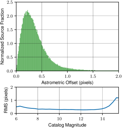
Figure 13: (top) Astrometric localization performance for the EFTE pipeline, and the RMS localization scatter as a function of magnitude (bottom). Performance is sub-pixel at the 99th percentile, with a typical RMS scatter of 7″, excepting stars brighter than 7th magnitude, which are typically saturated, and dimmer than 14th magnitude, where source confusion dominates in the source extraction.

5.3 vetnet Model Evaluation

We evaluated the vetnet real-bogus model using both the held-back test set described in Section 4.2.4, and an injection-recovery program over a sample of randomly selected images.

5.3.1 On-Sky Test Set

Figure 14 shows postage stamp cutouts and classification histograms from the held-back test set of on-sky transients, divided evenly between cases where vetnet classifcations and the human-assigned labels agreed and cases where they disagreed. In both categories, the entropy-based confidence score scales with subjective appraisal of the candidates; candidates (h), (k), (i), and (c) are faint borderline detections, assigned accordingly low confidence scores. Candidate (g) is a linear particle collision. Notably, candidates (f) and (l) have anomolously sharp PSFs that were both counted as real by human labellers, but were assigned bogus scores by the network, suggesting that they are morphologically more similar to cosmics. Even in cases where the labels are consistent, the confidence drops in areas with pathological PSFs, as in example (b), but particularly in example (a).

Figure 14: Sample on-sky candidates taken from the vetnet test set. “Actual” and “Pred” values represent sky truth class determined by a human inspector and the predicted class by the network, respectively. Histograms are an approximation of the normalized Bayesian posterior distribution for the probability of the candidate representing a real astrophysical event, quantified using the entropy-based $\mathbb{C}$ metric from Killestein et al. (2021). In cases where the sky truth and the network prediction disagree, $\mathbb{C}$ is typically $<0.5$, or extenuating circumstances exist, such as the anomolous PSFs in panels (l) and (f), or the potential human misclassifications in (h), (i), and (k).

Figure 15 shows the performance of the model on the on-sky test set. The magnitude-integrated precision and recall at a vetnet score threshold of 0.5 are 95.4% and 94.4% respectively, with a false positive rate of 5.1%. Depending on the science case and false-alarm tolerance of follow-up resources, these numbers can be tuned using a combination of the vetnet RB score and the $\mathbb{C}$ rating; for instance, a sub-percent FPR is measured above a RB threshold of 0.7.

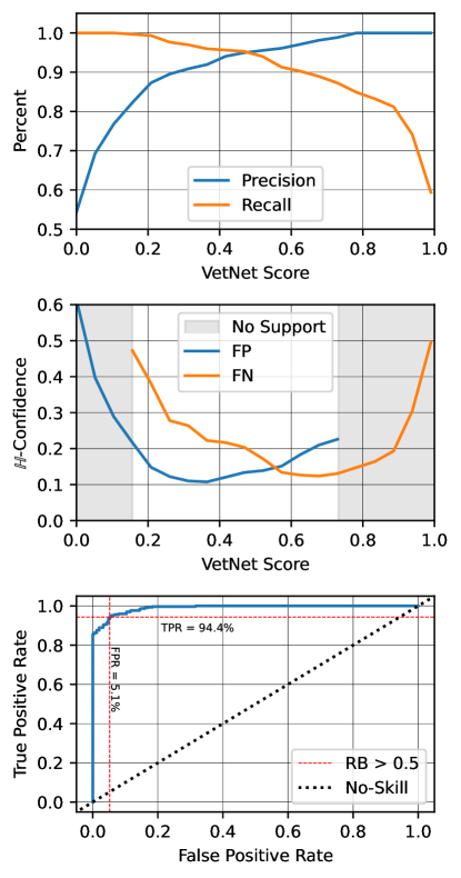
Figure 15: Performance of vetnet on the on-sky test set. (top) Precision and recall as a function of the vetnet real-bogus score. At the $RB=0.5$ threshold, the observed precision and recall are 95.4% and 94.4% respectively. (middle) Entropy-based confidence scores for false-positives and false-negatives as a function of vetnet real-bogus score threshold. Shaded regions indicate score regions where no false positives or false negatives occur within the on-sky test set. (bottom) ROC curve for vetnet. The area under the ROC curve (the ROC-AUC metric) is 0.99, representing the probability that a random real candidate will receive a higher real-bogus score than a random bogus candidate. No-skill line indicates the expected performance curve for a random classifier.

5.4 Candidate Production Latency

To enable rapid followup, EFTE must produce candidates on timescales comparable to the earliest and most impulsive phases of the astrophysical events of interest, ideally within the base cadence of the survey. For Evryscope, this means adding candidates to an actionable event stream within two minutes of the end of each exposure. We consider the candidate production latency as our figure of merit for speed, defined here as the time delay between the shutter close time for the image and candidates being fully inserted into the central EFTE database in Chapel Hill, with all automated vetting and in-database source association and deduplication actions complete.

Figure 16 presents histograms of candidate production latency for both Evryscope-North and Evryscope-South during early on-sky testing of EFTE between 25 November 2019 and 1 January 2020. Some variation is seen between Evryscope-North and Evryscope-South, which we attribute to a combination of the difference in on-site compute hardware specifications, camera counts, and varying network connectivity to each observatory.

Figure 16: Cumulative histogram (a) and distribution (b) of time delay between exposure and insertion of vetted candidates into the remote database between 25 November 2019 and 1 January 2020. 98.5% of images are fully reduced into lists of transient candidates within 120 seconds, before the next image is complete.

Cumulatively between both sites, EFTE is able to meet the sub-cadence latency requirement for 98.5% of images.

5.5 Injection-Recovery Testing for Completeness

To estimate the expected completeness of the survey, we selected 800 images from the 2021 Evryscope-North data set at random and injected simulated sources using the routine described in Section 4.2.5, and evaluated the recovery probability as a function of magnitude using the routine described in Corbett et al. (2020). The ratio of variables (injected with a minimum contrast of 0.25 mag) to transients without a counterpart in the reference image was 1:6. In total, 960,000 transients were added to the images.

Figure 17 shows the fraction of simulated transients recovered from the test set, and the corresponding recovery fraction from Corbett et al. (2020), which used an earlier version of the vetnet model. We note that dropping the vetnet-RB score threshold to 0.0 has a marginal effect on the dim end recovery curve, indicating that the decreased depth (50% at $m_{g}=14$ instead of 50% at $m_{g}=14.2$) is a property of the slightly different image sample rather than of the updated vetnet model.

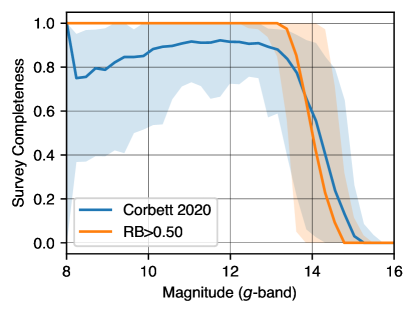
Figure 17: Survey completeness as a function of magnitude for both the current EFTE with a threshold vetnet real-bogus score of 0.5, and the previous version described in Corbett et al. (2020). Completeness is measured on a synthetic sample of injected transient and variable sources. Recovery probability for sources brighter than $m_{g}=13.2$ is 99.9%, and rapidly falls to 50% at $m_{g}=14$. Shaded regions represent the 90% confidence intervals of each curve, based on the percentiles of the per-image recovery functions.

Sources brighter than $m_{g}=13.2$ are successfully recovered in all images.

6 Science Results from EFTE

6.1 Rapid Follow-Up of Stellar Flares with SOAR

EFTE’s latency is fast enough for flare candidates to be observed by other telescopes in the minutes immediately following the flare’s detection. The Southern Astrophysical Research (SOAR) telescope is a 4.1-m telescope located at Cerro Pachon in Chile, which hosts the Goodman High-Throughput Spectrograph (Clemens et al., 2004). The entirety of Evryscope-South’s field of view is within SOAR’s observable area, and a band of Evryscope-North’s field of view below declinations of 10 degrees is accessible to SOAR. Ongoing studies pair SOAR and Goodman with the EFTE alert stream to acquire spectra of stellar flares within minutes of the flare’s detection, allowing the spectral evolution of flares to be characterized during the most impulsive phases of the flare with time resolution limited by the exposure time necessary to obtain a spectrum with adequate signal to noise ratio (typically sub-minute for EFTE-detected stellar flares).

6.1.1 EVRT-3586872, a $\Delta{m}=4.2$ Flare from a mid-M Dwarf

In an exposure beginning at 5:39:56 UTC on 15 February 2020, EFTE detected a new source from Evryscope South, which was then confirmed in the two consecutive images, at magnitudes 12.7 and 12.8 respectively, indicating that this source was both astrophysical in nature and potentially detected near its peak. The source, assigned the identifier EVRT-3586872, crossmatched to a star in the ATLAS reference catalog with a red color ($g-r=1.186$), suggesting a possible M-dwarf origin. The offset between the catalog star, 2MASS08593584-2340201, and the EFTE detection is 4.0 arcseconds, well within the expected astrometric error. The star is also cataloged in Heinze et al. (2018) as an irregular sinusoidal variable, consistent with an M-dwarf rotational signature.

Upon receiving a notification of consecutive detections of a cataloged red source via our web interface, we worked with SOAR staff to slew to its location, and began observing the target 14.9 minutes after the end of the first Evryscope detection image. We used the 400 line grating in the M1 configuration, covering approximately the wavelength range from 300 to 705 nm. Figure 18 shows a spectrum of the flare extracted from a 120-second exposure +15 minutes after the initial trigger, flux calibrated to the spectrum of LTT2445 (Hamuy et al., 1992, 1994).

We fit a two-component scaled blackbody model to the flare spectrum. This includes both a fixed contribution from the quiescent star, based on the Bayesian estimate of $T_{eff}$ from StarHorse2 (Anders et al., 2022), and thermal flare emission with a best-fit temperature of 22,852 K. At almost 23,000 K, this temperature is larger than typically assumed in flare models (Osten & Wolk, 2015), but consistent with temperatures recently inferred from broad-band light curves from TESS and Evryscope (Howard et al., 2020). We also note this measurement is subject to known systematics, including Balmer continuum emission features (Kowalski et al., 2013) and increasing uncertainty as true temperature increases, due to the optical bandpass primarily sampling the Rayleigh–Jeans tail of the spectrum at temperatures beyond $10^{4}$ K (Arcavi, 2022). Analysis of results from the EFTE-SOAR followup program is ongoing.

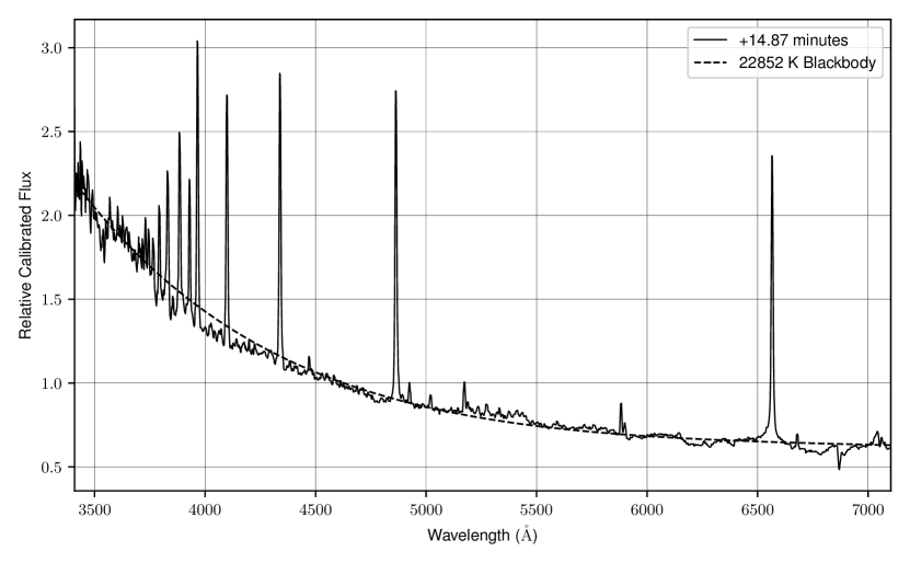
Figure 18: Spectrum of EVRT-3586872 at +14.87 minutes from the end of the first Evryscope detection of a flare candidate. The spectrum has been flux calibrated and normalized. The overlaid curve is a two-component blackbody spectrum consisting of a fitted 22852 K flare continuum and a 3256 K quiescent thermal spectrum.

6.2 EFTE Light Curves

In addition to transient alerts, EFTE enables users to produce long-term light curves for targets not included in the input catalog used for the Evryscope high-precision forced photometry pipeline (Ratzloff et al., 2019). EFTE light curves have been included in multiple publications, both by the Evryscope team and external collaborators. Publications using EFTE light curves include analyses of the galactic novae V1674 Her (Quimby et al., 2021) and V906 Car (Wee et al., 2020), measurements of the rotation periods of TESS exoplanet hosts, including one example with a 2.1 mmag amplitude measured from EFTE photometry (Howard et al., 2021), and long-term monitoring of a mysterious dust-emitting object orbiting the star TIC 400799224 (Powell et al., 2021).

6.3 Satellite Glint Foregrounds for Fast Transient Surveys

Image contamination by Earth artificial satellites takes two forms: streaks, with uniform illumination over extended trajectories, and glints, which appear as short-duration flashes. These two morphologies are frequently degenerate, and depend on the structure and orbit of the reflector. Short durations relative to their motion on the sky and sharp contrast with their associated streaks have led to glints being mistaken for astrophysical events (Schaefer et al., 1987; Maley, 1987, 1991; Rast, 1991; Shamir & Nemiroff, 2006). During the first six months of EFTE operations, we identified 1,415,722 likely satellite glints, and modeled an all-sky event rate of $1800^{+600}_{-280}$ sky^-1 hour^-1, peaking at $m_{g}=13.0$ (Corbett et al., 2020). This rate is orders of magnitude higher than the combined rate of public alerts from all active all-sky fast-timescale transient searches, including neutrino, gravitational-wave, gamma-ray, and radio observatories. A subsequent study, using the Weizmann Fast Astronomical Survey Telescope (W-FAST; Nir et al., 2020) revealed that this event rate increases sharply with depth, reporting an event rate of $9100^{+3000}_{-2000}$ sky^-1 hour^-1 for $9<M_{BP}<11$ around the equator, 2.3$\times$ the value we measured for ${m_{g}}<9$. As the majority of the events observed by Evryscope appear to be generated in low Earth orbit (LEO), we expect the event rate for satellite glints to correlate with the rapidly-growning number of LEO satellites.

7 Summary and Conclusions

In this paper, we presented the Evryscope Fast Transient Engine (EFTE), the real-time transient discovery pipeline for the Evryscopes. The pipeline is a fully custom data analysis tool, suited to the unique parameter space inhabited by the Evryscopes and capable of identifying transient candidates in real-time, with alerts available for each image within the two-minute cadence of the Evryscopes for 98.5% of images. To accomplish this, we reduce the complex image subtraction process adopted by seeing-limited surveys to a simple direct subtraction of near-consecutive images. Astrometric performance for transient alerts is sub-pixel at the 99th percentile, and photometric performance is within 0.06 mag RMS of the ATLAS-REFCAT2 catalog for reference stars within the $8<m_{g}<14.5$ sensitivity range of the survey. Using a convolutional real-bogus classifier, we are able to recover 99.9% of sources brighter than $m_{g}=13.2$ with a false positive rate of 5.1%.

While EFTE is specifically adapted to Evryscope data, the infrastructure, algorithms, and ML models, were developed to enable portability to instruments with similar survey strategies, such as the NASA Transiting Exoplanet Survey Satellite (TESS; Ricker et al., 2014), or with stringent data throughput and reduction latency requirements. Core algorithms from EFTE have been adapted for usage in the pipeline of the Argus Optical Array, a 5-meter class multiplexed 55 GPix synoptic survey instrument currently in development (Law et al., 2021, 2022). Argus will observe a field of view equivalent to Evryscope in alternating 1- and 30-second cadences, which produce up to 4.3 PiB and 145 TiB of raw data per night, respectively. To support this data rate, Argus data will be reduced in real time, producing low-latency transient alerts, photometry, and calibrated image data for distribution and storage. In Corbett et al. (2022a), we describe the Argus pipeline and data products, and demonstrate the direct subtraction algorithm described in Section 3.3 on the Argus Array Technology Demonstrator (Corbett et al., 2022b). The VETNET model described in Section 4 was optimized for direct image subtraction and Evryscope data; however, the framework for performing this optimization and for staged model training using both on-sky and simulated data is similarly portable to Argus.

A public alert stream from EFTE is in development, based on the evolving community standard, in use for the Zwicky Alert Distribution System (Patterson et al., 2019) and planned for the Rubin Observatory’s Legacy Survey of Space and Time (LSST), of serialized alert packets distributed via Apache Kafka (Kreps et al., 2011). Alerts will be available via the Arizona-NOIRLab Temporal Analysis and Response to Events System (ANTARES; Matheson et al., 2021). Details of the alert distribution system and alert schema contents will be addressed in future work.

References

- Abadi et al. (2015) Abadi, M., Agarwal, A., Barham, P., et al. 2015, TensorFlow: Large-Scale Machine Learning on Heterogeneous Systems. https://www.tensorflow.org/
- Abbott et al. (2009) Abbott, B. P., Abbott, R., Adhikari, R., et al. 2009, Reports on Progress in Physics, 72, 076901, doi: 10.1088/0034-4885/72/7/076901
- Agarap (2018) Agarap, A. F. 2018, arXiv preprint arXiv:1803.08375
- Aizawa et al. (2022) Aizawa, M., Kawana, K., Kashiyama, K., et al. 2022, PASJ, 74, 1069, doi: 10.1093/pasj/psac056
- Alard & Lupton (1998) Alard, C., & Lupton, R. H. 1998, ApJ, 503, 325, doi: 10.1086/305984
- Aldering et al. (2002) Aldering, G., Adam, G., Antilogus, P., et al. 2002, in Society of Photo-Optical Instrumentation Engineers (SPIE) Conference Series, Vol. 4836, Survey and Other Telescope Technologies and Discoveries, ed. J. A. Tyson & S. Wolff, 61–72, doi: 10.1117/12.458107
- Anders et al. (2022) Anders, F., Khalatyan, A., Queiroz, A. B. A., et al. 2022, A&A, 658, A91, doi: 10.1051/0004-6361/202142369
- Anderson & King (2000) Anderson, J., & King, I. R. 2000, PASP, 112, 1360, doi: 10.1086/316632
- Andreoni et al. (2017) Andreoni, I., Jacobs, C., Hegarty, S., et al. 2017, PASA, 34, e037, doi: 10.1017/pasa.2017.33
- Andreoni et al. (2020a) Andreoni, I., Cooke, J., Webb, S., et al. 2020a, MNRAS, 491, 5852, doi: 10.1093/mnras/stz3381
- Andreoni et al. (2020b) —. 2020b, MNRAS, 491, 5852, doi: 10.1093/mnras/stz3381
- Arcavi (2022) Arcavi, I. 2022, ApJ, 937, 75, doi: 10.3847/1538-4357/ac90c0
- Arimatsu et al. (2021) Arimatsu, K., Tsumura, K., Usui, F., Ootsubo, T., & Watanabe, J.-i. 2021, AJ, 161, 135, doi: 10.3847/1538-3881/abd94d
- Astropy Collaboration et al. (2013) Astropy Collaboration, Robitaille, T. P., Tollerud, E. J., et al. 2013, A&A, 558, A33, doi: 10.1051/0004-6361/201322068
- Astropy Collaboration et al. (2018) Astropy Collaboration, Price-Whelan, A. M., Sipőcz, B. M., et al. 2018, AJ, 156, 123, doi: 10.3847/1538-3881/aabc4f
- Bailey et al. (2008) Bailey, S., Aragon, C., Romano, R., et al. 2008, Astronomische Nachrichten, 329, 292, doi: 10.1002/asna.200710932
- Barbary (2016) Barbary, K. 2016, Journal of Open Source Software, 1, 58, doi: 10.21105/joss.00058
- Becker (2015) Becker, A. 2015, HOTPANTS: High Order Transform of PSF ANd Template Subtraction. http://ascl.net/1504.004
- Behnel et al. (2011) Behnel, S., Bradshaw, R., Citro, C., et al. 2011, Computing in Science & Engineering, 13, 31
- Bellm et al. (2019) Bellm, E. C., Kulkarni, S. R., Graham, M. J., et al. 2019, PASP, 131, 018002, doi: 10.1088/1538-3873/aaecbe
- Berger et al. (2013) Berger, E., Leibler, C. N., Chornock, R., et al. 2013, ApJ, 779, 18, doi: 10.1088/0004-637X/779/1/18
- Beroiz et al. (2020) Beroiz, M., Cabral, J., & Sanchez, B. 2020, Astronomy and Computing, 32, 100384, doi: https://doi.org/10.1016/j.ascom.2020.100384
- Bersten et al. (2018) Bersten, M. C., Folatelli, G., García, F., et al. 2018, Nature, 554, 497, doi: 10.1038/nature25151
- Bertin (2011) Bertin, E. 2011, in Astronomical Society of the Pacific Conference Series, Vol. 442, Astronomical Data Analysis Software and Systems XX, ed. I. N. Evans, A. Accomazzi, D. J. Mink, & A. H. Rots, 435
- Bertin & Arnouts (1996) Bertin, E., & Arnouts, S. 1996, A&AS, 117, 393, doi: 10.1051/aas:1996164
- Bhat et al. (2009) Bhat, P. N., Meegan, C. A., Lichti, G. G., et al. 2009, in American Institute of Physics Conference Series, Vol. 1133, American Institute of Physics Conference Series, ed. C. Meegan, C. Kouveliotou, & N. Gehrels, 34–36, doi: 10.1063/1.3155916
- Bloom et al. (2008) Bloom, J. S., Starr, D. L., Butler, N. R., et al. 2008, Astronomische Nachrichten, 329, 284, doi: 10.1002/asna.200710957
- Bramich (2008) Bramich, D. 2008, Monthly Notices of the Royal Astronomical Society, 386, doi: 10.1111/j.1745-3933.2008.00464.x
- Brink et al. (2013) Brink, H., Richards, J. W., Poznanski, D., et al. 2013, MNRAS, 435, 1047, doi: 10.1093/mnras/stt1306
- Burke et al. (2019) Burke, C. J., Aleo, P. D., Chen, Y.-C., et al. 2019, MNRAS, 490, 3952, doi: 10.1093/mnras/stz2845
- Butler et al. (2016) Butler, H., Daly, M., Doyle, A., et al. 2016, The GeoJSON Format, doi: 10.17487/RFC7946
- Bäuerle et al. (2021) Bäuerle, A., van Onzenoodt, C., & Ropinski, T. 2021, IEEE Transactions on Visualization and Computer Graphics, 27, 2980, doi: 10.1109/TVCG.2021.3057483
- Calabretta et al. (2004) Calabretta, M. R., Valdes, F., Greisen, E. W., & Allen, S. L. 2004, in Astronomical Society of the Pacific Conference Series, Vol. 314, Astronomical Data Analysis Software and Systems (ADASS) XIII, ed. F. Ochsenbein, M. G. Allen, & D. Egret, 551
- Cao et al. (2016) Cao, Y., Nugent, P. E., & Kasliwal, M. M. 2016, arXiv, doi: 10.1088/1538-3873/128/969/114502
- Chollet et al. (2015) Chollet, F., et al. 2015, Keras, GitHub. https://github.com/fchollet/keras
- Clemens et al. (2004) Clemens, J. C., Crain, J. A., & Anderson, R. 2004, in Society of Photo-Optical Instrumentation Engineers (SPIE) Conference Series, Vol. 5492, Ground-based Instrumentation for Astronomy, ed. A. F. M. Moorwood & M. Iye, 331–340, doi: 10.1117/12.550069
- Corbett et al. (2022a) Corbett, H., Soto, A. V., Machia, L., et al. 2022a, in Software and Cyberinfrastructure for Astronomy VII, ed. J. Ibsen & G. Chiozzi, Vol. 12189, International Society for Optics and Photonics (SPIE), 1218910, doi: 10.1117/12.2629533
- Corbett et al. (2022b) Corbett, H., Soto, A. V., Machia, L., et al. 2022b, in Ground-based and Airborne Telescopes IX, ed. H. K. Marshall, J. Spyromilio, & T. Usuda, Vol. 12182, International Society for Optics and Photonics (SPIE), 121824D, doi: 10.1117/12.2629489
- Corbett et al. (2022) Corbett, H., Vasquez Soto, A., Machia, L., et al. 2022, in Society of Photo-Optical Instrumentation Engineers (SPIE) Conference Series, Vol. 12189, Society of Photo-Optical Instrumentation Engineers (SPIE) Conference Series, 1218910, doi: 10.1117/12.2629533
- Corbett et al. (2020) Corbett, H., Law, N. M., Soto, A. V., et al. 2020, ApJ, 903, L27, doi: 10.3847/2041-8213/abbee5
- Cucchiara et al. (2011) Cucchiara, A., Cenko, S. B., Bloom, J. S., et al. 2011, ApJ, 743, 154, doi: 10.1088/0004-637X/743/2/154
- Dálya et al. (2018) Dálya, G., Galgóczi, G., Dobos, L., et al. 2018, Monthly Notices of the Royal Astronomical Society, 479, 2374, doi: 10.1093/mnras/sty1703
- Dark Energy Survey Collaboration et al. (2016) Dark Energy Survey Collaboration, Abbott, T., Abdalla, F. B., et al. 2016, Monthly Notices of the Royal Astronomical Society, 460, 1270, doi: 10.1093/mnras/stw641
- Dieleman et al. (2015) Dieleman, S., Willett, K. W., & Dambre, J. 2015, MNRAS, 450, 1441, doi: 10.1093/mnras/stv632
- Drake et al. (2009) Drake, A. J., Djorgovski, S. G., Mahabal, A., et al. 2009, ApJ, 696, 870, doi: 10.1088/0004-637X/696/1/870
- Duev et al. (2019) Duev, D. A., Mahabal, A., Masci, F. J., et al. 2019, MNRAS, 489, 3582, doi: 10.1093/mnras/stz2357
- Dyer et al. (2018) Dyer, M. J., Dhillon, V. S., Littlefair, S., et al. 2018, in Society of Photo-Optical Instrumentation Engineers (SPIE) Conference Series, Vol. 10704, Observatory Operations: Strategies, Processes, and Systems VII, 107040C, doi: 10.1117/12.2311865
- Fischler & Bolles (1981) Fischler, M., & Bolles, R. 1981, Communications of the ACM, 24, 381. /brokenurl#http://publication.wilsonwong.me/load.php?id=233282275
- Flewelling et al. (2016) Flewelling, H. A., Magnier, E. A., Chambers, K. C., et al. 2016, arXiv e-prints, arXiv:1612.05243. https://arxiv.org/abs/1612.05243
- Fox et al. (2003) Fox, D. W., Price, P. A., Soderberg, A. M., et al. 2003, ApJ, 586, L5, doi: 10.1086/374683
- Fresneau & Osborn (2009) Fresneau, A., & Osborn, W. H. 2009, A&A, 503, 1023, doi: 10.1051/0004-6361/200810798
- Förster et al. (2016) Förster, F., Maureira, J. C., Martín, J. S., et al. 2016, arXiv, doi: 10.3847/0004-637x/832/2/155
- Gaia Collaboration et al. (2018) Gaia Collaboration, Brown, A. G. A., Vallenari, A., et al. 2018, A&A, 616, A1, doi: 10.1051/0004-6361/201833051
- Gal & Ghahramani (2015a) Gal, Y., & Ghahramani, Z. 2015a, arXiv e-prints, arXiv:1506.02142. https://arxiv.org/abs/1506.02142
- Gal & Ghahramani (2015b) —. 2015b, arXiv e-prints, arXiv:1506.02158. https://arxiv.org/abs/1506.02158
- Garnavich et al. (2016) Garnavich, P. M., Tucker, B. E., Rest, A., et al. 2016, ApJ, 820, 23, doi: 10.3847/0004-637X/820/1/23
- Ghosh et al. (2016) Ghosh, A., Manwani, N., & Sastry, P. S. 2016, arXiv e-prints, arXiv:1605.06296. https://arxiv.org/abs/1605.06296
- Goldstein et al. (2015) Goldstein, D. A., D’Andrea, C. B., Fischer, J. A., et al. 2015, AJ, 150, 82, doi: 10.1088/0004-6256/150/3/82
- Górski & Hivon (2011) Górski, K. M., & Hivon, E. 2011, HEALPix: Hierarchical Equal Area isoLatitude Pixelization of a sphere, Astrophysics Source Code Library, record ascl:1107.018. http://ascl.net/1107.018
- Hamuy et al. (1994) Hamuy, M., Suntzeff, N. B., Heathcote, S. R., et al. 1994, PASP, 106, 566, doi: 10.1086/133417
- Hamuy et al. (1992) Hamuy, M., Walker, A. R., Suntzeff, N. B., et al. 1992, PASP, 104, 533, doi: 10.1086/133028
- Hedges et al. (2021) Hedges, C., Luger, R., Martinez-Palomera, J., Dotson, J., & Barentsen, G. 2021, AJ, 162, 107, doi: 10.3847/1538-3881/ac0825
- Heinze et al. (2018) Heinze, A. N., Tonry, J. L., Denneau, L., et al. 2018, AJ, 156, 241, doi: 10.3847/1538-3881/aae47f
- Henden et al. (2016) Henden, A. A., Templeton, M., Terrell, D., et al. 2016, VizieR Online Data Catalog, II/336
- Ho et al. (2018) Ho, A. Y. Q., Kulkarni, S. R., Nugent, P. E., et al. 2018, ApJ, 854, L13, doi: 10.3847/2041-8213/aaaa62
- Hoffleit & Jaschek (1991) Hoffleit, D., & Jaschek, C. 1991, The Bright star catalogue (Yale University Observatory)
- Høg et al. (2000) Høg, E., Fabricius, C., Makarov, V. V., et al. 2000, A&A, 355, L27
- Howard & MacGregor (2022) Howard, W. S., & MacGregor, M. A. 2022, ApJ, 926, 204, doi: 10.3847/1538-4357/ac426e
- Howard et al. (2018) Howard, W. S., Tilley, M. A., Corbett, H., et al. 2018, ApJ, 860, L30, doi: 10.3847/2041-8213/aacaf3
- Howard et al. (2020) Howard, W. S., Corbett, H., Law, N. M., et al. 2020, ApJ, 902, 115, doi: 10.3847/1538-4357/abb5b4
- Howard et al. (2021) Howard, W. S., Teske, J., Corbett, H., et al. 2021, AJ, 162, 147, doi: 10.3847/1538-3881/ac0fe3
- Hu et al. (2022) Hu, L., Wang, L., Chen, X., & Yang, J. 2022, ApJ, 936, 157, doi: 10.3847/1538-4357/ac7394
- Ioffe & Szegedy (2015) Ioffe, S., & Szegedy, C. 2015, arXiv e-prints, arXiv:1502.03167. https://arxiv.org/abs/1502.03167
- Jayasinghe et al. (2018) Jayasinghe, T., Kochanek, C. S., Stanek, K. Z., et al. 2018, MNRAS, 477, 3145, doi: 10.1093/mnras/sty838
- Kaiser et al. (2010) Kaiser, N., Burgett, W., Chambers, K., et al. 2010, in Society of Photo-Optical Instrumentation Engineers (SPIE) Conference Series, Vol. 7733, Proc. SPIE, 77330E, doi: 10.1117/12.859188
- Keller et al. (2007) Keller, S. C., Schmidt, B. P., Bessell, M. S., et al. 2007, PASA, 24, 1, doi: 10.1071/AS07001
- Killestein et al. (2021) Killestein, T. L., Lyman, J., Steeghs, D., et al. 2021, MNRAS, 503, 4838, doi: 10.1093/mnras/stab633
- Kingma & Ba (2014) Kingma, D. P., & Ba, J. 2014, arXiv e-prints, arXiv:1412.6980. https://arxiv.org/abs/1412.6980
- Koposov & Bartunov (2006) Koposov, S., & Bartunov, O. 2006, in Astronomical Society of the Pacific Conference Series, Vol. 351, Astronomical Data Analysis Software and Systems XV, ed. C. Gabriel, C. Arviset, D. Ponz, & S. Enrique, 735
- Koposov & Bartunov (2019) Koposov, S., & Bartunov, O. 2019, Q3C: A PostgreSQL package for spatial queries and cross-matches of large astronomical catalogs. http://ascl.net/1905.008
- Kowalski et al. (2013) Kowalski, A. F., Hawley, S. L., Wisniewski, J. P., et al. 2013, ApJS, 207, 15, doi: 10.1088/0067-0049/207/1/15
- Kreps et al. (2011) Kreps, J., Narkhede, N., & Rao, J. 2011, in Proceedings of the NetDB, 1–7
- Kulkarni & Rau (2006) Kulkarni, S. R., & Rau, A. 2006, ApJ, 644, L63, doi: 10.1086/505423
- Kumar (1988) Kumar, M. 1988, Marine Geodesy, 12, 117
- Kumar et al. (2015) Kumar, S., Gezari, S., Heinis, S., et al. 2015, ApJ, 802, 27, doi: 10.1088/0004-637X/802/1/27
- Lang et al. (2010) Lang, D., Hogg, D. W., Mierle, K., Blanton, M., & Roweis, S. 2010, AJ, 139, 1782, doi: 10.1088/0004-6256/139/5/1782
- Larson et al. (2003) Larson, S., Beshore, E., Hill, R., et al. 2003, in AAS/Division for Planetary Sciences Meeting Abstracts #35, AAS/Division for Planetary Sciences Meeting Abstracts, 36.04
- Law et al. (2022) Law, N., Vasquez Soto, A., Corbett, H., et al. 2022, in Society of Photo-Optical Instrumentation Engineers (SPIE) Conference Series, Vol. 12182, Ground-based and Airborne Telescopes IX, ed. H. K. Marshall, J. Spyromilio, & T. Usuda, 121824H, doi: 10.1117/12.2630037
- Law et al. (2009) Law, N. M., Kulkarni, S. R., Dekany, R. G., et al. 2009, PASP, 121, 1395, doi: 10.1086/648598
- Law et al. (2015) Law, N. M., Fors, O., Ratzloff, J., et al. 2015, PASP, 127, 234, doi: 10.1086/680521
- Law et al. (2021) Law, N. M., Corbett, H., Galliher, N. W., et al. 2021, arXiv e-prints, arXiv:2107.00664. https://arxiv.org/abs/2107.00664
- Le Folgoc et al. (2021) Le Folgoc, L., Baltatzis, V., Desai, S., et al. 2021, arXiv e-prints, arXiv:2110.04286. https://arxiv.org/abs/2110.04286
- LeCun & Bengio (1995) LeCun, Y., & Bengio, Y. 1995, in The Handbook of Brain Theory and Neural Networks, ed. M. A. Arbib (MIT Press)
- LeCun et al. (1989) LeCun, Y., Boser, B., Denker, J. S., et al. 1989, Neural Computation, 1, 541
- Li et al. (2018) Li, L., Jamieson, K., DeSalvo, G., Rostamizadeh, A., & Talwalkar, A. 2018, Journal of Machine Learning Research, 18, 1. http://jmlr.org/papers/v18/16-558.html
- Lipunov et al. (2004) Lipunov, V. M., Krylov, A. V., Kornilov, V. G., et al. 2004, Astronomische Nachrichten, 325, 580, doi: 10.1002/asna.200410284
- Mahabal et al. (2019) Mahabal, A., Rebbapragada, U., Walters, R., et al. 2019, PASP, 131, 038002, doi: 10.1088/1538-3873/aaf3fa
- Makhlouf et al. (2021) Makhlouf, K., Turpin, D., Corre, D., et al. 2021, arXiv
- Maley (1991) Maley, P. 1991, Advances in Space Research, 11, 33–36, doi: 10.1016/0273-1177(91)90539-v
- Maley (1987) Maley, P. D. 1987, The Astrophysical Journal, 317, L39, doi: 10.1086/184909
- Martin-Carrillo et al. (2014) Martin-Carrillo, A., Hanlon, L., Topinka, M., et al. 2014, A&A, 567, A84, doi: 10.1051/0004-6361/201220872
- Matheson et al. (2021) Matheson, T., Stubens, C., Wolf, N., et al. 2021, AJ, 161, 107, doi: 10.3847/1538-3881/abd703
- Mcculloch & Pitts (1943) Mcculloch, W., & Pitts, W. 1943, Bulletin of Mathematical Biophysics, 5, 127
- Nir et al. (2020) Nir, G., Ofek, E. O., Ben-Ami, S., et al. 2020, arXiv e-prints, arXiv:2011.03497. https://arxiv.org/abs/2011.03497
- Osten & Wolk (2015) Osten, R. A., & Wolk, S. J. 2015, ApJ, 809, 79, doi: 10.1088/0004-637X/809/1/79
- Patterson et al. (2019) Patterson, M. T., Bellm, E. C., Rusholme, B., et al. 2019, PASP, 131, 018001, doi: 10.1088/1538-3873/aae904
- Perrett et al. (2010) Perrett, K., Balam, D., Sullivan, M., et al. 2010, The Astronomical Journal, 140, 518, doi: 10.1088/0004-6256/140/2/518
- Pickles & Depagne (2010) Pickles, A., & Depagne, É. 2010, PASP, 122, 1437, doi: 10.1086/657947
- Pietras et al. (2022) Pietras, M., Falewicz, R., Siarkowski, M., Bicz, K., & Preś, P. 2022, ApJ, 935, 143, doi: 10.3847/1538-4357/ac8352
- Powell et al. (2021) Powell, B. P., Kostov, V. B., Rappaport, S. A., et al. 2021, The Astronomical Journal, 162, 299, doi: 10.3847/1538-3881/ac2c81
- Quimby et al. (2021) Quimby, R. M., Shafter, A. W., & Corbett, H. 2021, Research Notes of the American Astronomical Society, 5, 160, doi: 10.3847/2515-5172/ac14c0
- Ranjan et al. (2017) Ranjan, S., Wordsworth, R., & Sasselov, D. D. 2017, ApJ, 843, 110, doi: 10.3847/1538-4357/aa773e
- Rast (1991) Rast, R. H. 1991, Icarus, 90, 328–329, doi: 10.1016/0019-1035(91)90112-7
- Ratzloff et al. (2020) Ratzloff, J. K., Law, N. M., Corbett, H. T., Fors, O., & del Ser, D. 2020, arXiv e-prints, arXiv:2001.00879. https://arxiv.org/abs/2001.00879
- Ratzloff et al. (2019) Ratzloff, J. K., Law, N. M., Fors, O., et al. 2019, PASP, 131, 075001, doi: 10.1088/1538-3873/ab19d0
- Richmond et al. (2020) Richmond, M. W., Tanaka, M., Morokuma, T., et al. 2020, PASJ, 72, 3, doi: 10.1093/pasj/psz120
- Ricker et al. (2014) Ricker, G. R., Winn, J. N., Vanderspek, R., et al. 2014, in Society of Photo-Optical Instrumentation Engineers (SPIE) Conference Series, Vol. 9143, Space Telescopes and Instrumentation 2014: Optical, Infrared, and Millimeter Wave, ed. J. Oschmann, Jacobus M., M. Clampin, G. G. Fazio, & H. A. MacEwen, 914320, doi: 10.1117/12.2063489
- Rolnick et al. (2017) Rolnick, D., Veit, A., Belongie, S., & Shavit, N. 2017, arXiv e-prints, arXiv:1705.10694. https://arxiv.org/abs/1705.10694
- Schaefer et al. (2000) Schaefer, B. E., King, J. R., & Deliyannis, C. P. 2000, ApJ, 529, 1026, doi: 10.1086/308325
- Schaefer et al. (1987) Schaefer, B. E., Barber, M., Brooks, J. J., et al. 1987, ApJ, 320, 398, doi: 10.1086/165552
- Segura et al. (2010) Segura, A., Walkowicz, L. M., Meadows, V., Kasting, J., & Hawley, S. 2010, Astrobiology, 10, 751, doi: 10.1089/ast.2009.0376
- Shamir & Nemiroff (2006) Shamir, L., & Nemiroff, R. J. 2006, PASP, 118, 1180, doi: 10.1086/506989
- Shappee et al. (2014) Shappee, B. J., Prieto, J. L., Grupe, D., et al. 2014, ApJ, 788, 48, doi: 10.1088/0004-637X/788/1/48
- Simonyan & Zisserman (2014) Simonyan, K., & Zisserman, A. 2014, arXiv e-prints, arXiv:1409.1556. https://arxiv.org/abs/1409.1556
- Srivastava et al. (2014) Srivastava, N., Hinton, G., Krizhevsky, A., Sutskever, I., & Salakhutdinov, R. 2014, Journal of Machine Learning Research, 15, 1929. http://jmlr.org/papers/v15/srivastava14a.html
- Stoppa et al. (2022) Stoppa, F., Vreeswijk, P., Bloemen, S., et al. 2022, arXiv e-prints, arXiv:2202.00489. https://arxiv.org/abs/2202.00489
- Tamuz et al. (2005) Tamuz, O., Mazeh, T., & Zucker, S. 2005, MNRAS, 356, 1466, doi: 10.1111/j.1365-2966.2004.08585.x
- Tonry et al. (2018) Tonry, J. L., Denneau, L., Heinze, A. N., et al. 2018, Publications of the Astronomical Society of the Pacific, 130, 064505, doi: 10.1088/1538-3873/aabadf
- Tonry et al. (2018) Tonry, J. L., Denneau, L., Flewelling, H., et al. 2018, ApJ, 867, 105, doi: 10.3847/1538-4357/aae386
- Troja et al. (2017) Troja, E., Lipunov, V. M., Mundell, C. G., et al. 2017, Nature, 547, 425, doi: 10.1038/nature23289
- van Roestel et al. (2019) van Roestel, J., Groot, P. J., Kupfer, T., et al. 2019, MNRAS, 484, 4507, doi: 10.1093/mnras/stz241
- Vestrand et al. (2014) Vestrand, W. T., Wren, J. A., Panaitescu, A., et al. 2014, Science, 343, 38, doi: 10.1126/science.1242316
- Voges et al. (1999) Voges, W., Aschenbach, B., Boller, T., et al. 1999, A&A, 349, 389. https://arxiv.org/abs/astro-ph/9909315
- Walkowicz et al. (2008) Walkowicz, L. M., Johns-Krull, C. M., & Hawley, S. L. 2008, The Astrophysical Journal, 677, 593, doi: 10.1086/526421
- Wang et al. (2021) Wang, J., Xin, L. P., Li, H. L., et al. 2021, ApJ, 916, 92, doi: 10.3847/1538-4357/ac096f
- Watson et al. (2020) Watson, C., Henden, A. A., & Price, A. 2020, VizieR Online Data Catalog, B/vsx
- Wee et al. (2020) Wee, J., Blagorodnova, N., Penprase, B. E., et al. 2020, ApJ, 899, 162, doi: 10.3847/1538-4357/aba3cc
- Wolf et al. (2018) Wolf, C., Onken, C. A., Luvaul, L. C., et al. 2018, PASA, 35, e010, doi: 10.1017/pasa.2018.5
- Xin et al. (2021) Xin, L. P., Li, H. L., Wang, J., et al. 2021, ApJ, 909, 106, doi: 10.3847/1538-4357/abdd1b
- Zackay et al. (2016) Zackay, B., Ofek, E. O., & Gal-Yam, A. 2016, ApJ, 830, 27, doi: 10.3847/0004-637X/830/1/27