Solution formula for the general birth-death chemical diffusion master equation

Abstract

We propose a solution formula for chemical diffusion master equations of birth and death type. These equations, proposed and formalized in the recent paper [5], aim at incorporating the spatial diffusion of molecules into the description provided by the classical chemical master equation. We start from the general approach developed in [20] and perform a more detailed analysis of the representation found there. This leads to a solution formula for birth-death chemical diffusion master equations which is expressed in terms of the solution to the reaction-diffusion partial differential equation associated with the system under investigation. Such representation also reveals a striking analogy with the solution to the classical birth-death chemical master equations. The solutions of our findings are also illustrated for several examples.

Key words and phrases: chemical diffusion master equation, Ornstein-Uhlenbeck process, Feynman-Kac formula, spectral methods.

AMS 2000 classification: 60H07; 60H30; 92E20.

1 Introduction and statement of the main results

The dynamics of biochemical processes in living cells are commonly understood as an interplay between the spatial transport (diffusion) of molecules and their chemical kinetics (reaction), both of which are inherently stochastic at the molecular scale. In the case of systems with small molecule numbers in spatially well-mixed settings, the diffusion is averaged out and the probabilistic dynamics are governed by the well-known chemical master equation (CME) [13, 23, 24]. The CME can be seldom solved analytically [16]. However, solving a few simple cases analytically can bring valuable insight to the solutions of more complex cases. Alternatively, one can solve it by integrating stochastic trajectories with the Gillespie or tau-leap algorithms [1, 13], by approximation methods [8, 11, 22, 25] or even by deep learning approaches [14, 17].

In the case of spatially inhomogeneous systems, where diffusion is not averaged out, one would expect to obtain a similar master equation. However, obtaining such an equation is plagued with mathematical difficulties, and although it was hinted in previous work [10] and formulated for some specific systems [26], it was not until recently that this was formalized into the so-called chemical diffusion master equation (CDME) [5, 7]. The CDME changes a few paradigms that have not yet been explored thoroughly in stochastic chemical kinetics models. It combines continuous and discrete degrees of freedom, and it models reaction and diffusion as a joint stochastic process. It consists of an infinite sorted family of Fokker-Planck equations, where each level of the sorted family corresponds to a certain number of particles/molecules. The equations at each level describe the spatial diffusion of the corresponding set of particles, and they are coupled to each other via reaction operators, which change the number of particles in the system. The CDME is the theoretical backbone of reaction-diffusion processes, and thus, it is fundamental to model and understand biochemical processes in living cells, as well as to develop multiscale numerical methods [6, 12, 19, 27] and hybrid algorithms [3, 9, 4]. The stochastic trajectories of the CDME can be often integrated using particle–based reaction–diffusion simulations [2, 15]. However, analytic and approximate solutions have not yet been explored in detail. In this work, we work out a method to obtain an analytic solution of the CDME for a simple birth-death reaction system, with the aim to bring insight of the CDME solution of more complex systems.

We consider a system of indistinguishable molecules of a chemical species $S$ which undergo

• diffusion in the bounded open region $\mathbb{X}$ of $\mathbb{R}^{3}$;

• degradation and creation chemical reactions

  $$\mbox{(I)}\quad S\xrightarrow{\lambda_{d}(x)}\varnothing\quad\quad\quad\mbox{(II)}\quad\varnothing\xrightarrow{\lambda_{c}(x)}S,$$

  where $\lambda_{d}(x)$ denotes the propensity for reaction (I) to occur for a particle located at position $x\in\mathbb{X}$ (i.e., the probability per unit of time for this particle to disappear) while $\lambda_{c}(x)$ is the propensity for a new particle to be created at position $x\in\mathbb{X}$ by reaction (II).

To describe the evolution in time of such system the authors in [5, 7] proposed a set of equations for the number and position of the molecules. Namely, for $t\geq 0$, $n\geq 1$ and $A\in\mathcal{B}(\mathbb{X}^{n})$ they set

$$\mathcal{N}(t) :=\mbox{ number of molecules at time $t$},$$

$$\rho_{0}(t) :=\mathbb{P}(\mathcal{N}(t)=0)$$

$$\int_{A}\rho_{n}(t,x_{1},...,x_{n})dx_{1}\cdot\cdot\cdot dx_{n} :=\mathbb{P}\left(\{\mathcal{N}(t)=n\}\cap\{(X_{1}(t),...,X_{n}(t))\in A\}\right);$$

here, $dx_{i}$ stands for the three dimensional integration volume $dx^{(1)}_{i}dx^{(2)}_{i}dx^{(3)}_{i}$. Then, according to [5, 7] the time evolution of the reaction-diffusion process described above is governed by the following infinite system of equations:

$$\begin{cases}\begin{split}\partial_{t}\rho_{n}(t,x_{1},...,x_{n})=&\sum_{i=1}^{n}\Delta_{i}\rho_{n}(t,x_{1},...,x_{n})\\ &+(n+1)\int_{\mathbb{X}}\lambda_{d}(y)\rho_{n+1}(t,x_{1},...,x_{n},y)dy\\ &-\sum_{i=1}^{n}\lambda_{d}(x_{i})\rho_{n}(t,x_{1},...,x_{n})\\ &+\frac{1}{n}\sum_{i=1}^{n}\lambda_{c}(x_{i})\rho_{n-1}(t,x_{1},...,x_{i-1},x_{i+1},...,x_{n})\\ &-\int_{\mathbb{X}}\lambda_{c}(y)dy\cdot\rho_{n}(t,x_{1},...,x_{n}),\quad\quad\quad n\geq 0,t>0,(x_{1},...,x_{n})\in\mathbb{X}^{n};\end{split}\end{cases}$$ (1.1)

where we agree on assigning value zero to the three sums above when $n=0$. The term

$$\sum_{i=1}^{n}\Delta_{i}\rho_{n}(t,x_{1},...,x_{n})$$

in (1.1) refers to spatial diffusion of the particles: here,

$$\Delta_{i}:=\partial^{2}_{x_{i}^{(1)}}+\partial^{2}_{x_{i}^{(2)}}+\partial^{2}_{x_{i}^{(3)}}$$

stands for the three dimensional Laplace operator. We remark that to ease the notation we choose a driftless isotropic diffusion but the extension to the divergence-form second order partial differential operator

$$\mathtt{L}_{x_{i}}v:=\sum_{l,m=1}^{3}\partial_{x^{(l)}_{i}}\left(a_{lm}(x_{i})\partial_{x^{(m)}_{i}}v\right)-\sum_{l=1}^{3}\partial_{x^{(l)}_{i}}\left(b_{l}(x_{i})v\right),$$

which models a general anisotropic diffusion with drift on $\mathbb{R}^{3}$, is readily obtained. The terms

$$(n+1)\int_{\mathbb{X}}\lambda_{d}(y)\rho_{n+1}(t,x_{1},...,x_{n},y)dy-\sum_{i=1}^{n}\lambda_{d}(x_{i})\rho_{n}(t,x_{1},...,x_{n})$$

formalize gain and loss, respectively, due to reaction (I), while

$$\frac{1}{n}\sum_{i=1}^{n}\lambda_{c}(x_{i})\rho_{n-1}(t,x_{1},...,x_{i-1},x_{i+1},...,x_{n})-\int_{\mathbb{X}}\lambda_{c}(y)dy\cdot\rho_{n}(t,x_{1},...,x_{n})$$

relate to reaction (II). System (1.1) is combined with initial and Neumann boundary conditions

$$\begin{cases}\begin{split}\rho_{0}(0)&=1;\\ \rho_{n}(0,x_{1},...,x_{n})&=0,\quad n\geq 1,(x_{1},...,x_{n})\in\mathbb{X}^{n};\\ \partial_{\nu}\rho_{n}(t,x_{1},...,x_{n})&=0,\quad n\geq 1,t\geq 0,(x_{1},...,x_{n})\in\partial\mathbb{X}^{n}.\end{split}\end{cases}$$ (1.2)

The initial condition above states that there are no molecules in the system at time zero while the Neumann condition prevents flux through the boundary of $\mathbb{X}$, thus forcing the diffusion of the molecules inside $\mathbb{X}$. The symbol $\partial_{\nu}$ in (1.2) stands for the directional derivative along the outer normal vector at the boundary of $\mathbb{X}^{n}$.

Aim of this note is to present the following solution formula for (1.1)-(1.2).

Theorem 1.1.

Let $v$ be a classical solution of the problem

$$\begin{cases}\partial_{t}v(t,x)=\Delta v(t,x)-\lambda_{d}(x)v(t,x)+\lambda_{c}(x),&t>0,x\in\mathbb{X};\\ v(0,x)=0,&x\in\bar{\mathbb{X}};\\ \partial_{\nu}v(t,x)=0,&t\geq 0,x\in\partial\mathbb{X}.\end{cases}$$ (1.3)

Then, the chemical diffusion master equation (1.1) with initial and boundary conditions (1.2) has a classical solution given by

$$\rho_{0}(t)=\mathbb{P}(\mathcal{N}(t)=0)=\exp\left\{-\int_{\mathbb{X}}v(t,x)dx\right\},\quad t\geq 0,$$ (1.4)

and for $n\geq 1$

$$\rho_{n}(t,x_{1},...,x_{n})=\exp\left\{-\int_{\mathbb{X}}v(t,x)dx\right\}\frac{1}{n!}v(t,x_{1})\cdot\cdot\cdot v(t,x_{n}),\quad t\geq 0,(x_{1},...,x_{n})\in\mathbb{X}^{n}.$$ (1.5)

To prove the validity of the representations (1.4)-(1.5) one can trivially differentiate the right hand sides with respect to $t$ and verify using (1.3) that they indeed solve (1.1)-(1.2). We will however provide in the next section a constructive derivation of the expressions (1.4)-(1.5) which is based on the general approach proposed in [20]; here, an infinite dimensional version of the moment generating function method, which is commonly utilized to solve analytically some chemical master equations (see for details [21]), is developed. These techniques are also employed in an ongoing work which consider chemical diffusion master equations with higher order reactions.

Remark 1.2.

It is important to highlight the striking similarities between the representation formulas (1.4)-(1.5) for the solution of the CDME (1.1)-(1.2) and the solution

$$\varphi_{n}(t)=\frac{\left(\frac{\mathtt{c}}{\mathtt{d}}(1-e^{-\mathtt{d}t})\right)^{n}}{n!}e^{-\frac{\mathtt{c}}{\mathtt{d}}(1-e^{-\mathtt{d}t})},\quad t\geq 0,n\geq 0,$$ (1.6)

of the corresponding (diffusion-free) birth-death chemical master equation

$$\dot{\varphi}_{n}(t)=\mathtt{d}(n+1)\varphi_{n+1}(t)+\mathtt{c}\varphi_{n-1}(t)-\mathtt{d}n\varphi_{n}(t)-\mathtt{c}\varphi_{n}(t),$$ (1.7)

with initial condition

$$\varphi_{n}(0)=\delta_{0n},\quad\mbox{for all }n\geq 0.$$ (1.8)

Equation (1.7)-(1.8) describes the evolution in time of the probability

$$\varphi_{n}(t):=\mathbb{P}(\emph{number of molecules at time $t$}=n)$$

for the reactions

$$\emph{(I)}\quad S\xrightarrow{\mathtt{d}}\varnothing\quad\quad\quad\emph{(II)}\quad\varnothing\xrightarrow{\mathtt{c}}S,$$

with no molecules at time zero. Here, $\mathtt{d}$ and $\mathtt{c}$ are the stochastic rate constants for degradation and creation reactions, respectively. (To see how (1.6) is derived from (1.7)-(1.8) one can for instance use the moment generating function method: see [21] for details). We note that the function

$$t\mapsto\frac{\mathtt{c}}{\mathtt{d}}(1-e^{-\mathtt{d}t}),$$

appearing in (1.6) solves the deterministic rate equation

$$\begin{cases}\frac{d}{dt}v(t)=-\mathtt{d}v(t)+\mathtt{c},&t>0\\ v(0)=0&.\end{cases}$$ (1.9)

This establishes a perfect agreement between (1.3),(1.4),(1.5), i.e. representation of the solution for (1.1)-(1.2) and reaction-diffusion PDE, on one side and (1.6),(1.9), i.e. representation of the solution for (1.7)-(1.8) and rate equation, on the other side.

Corollary 1.3.

In the reaction-diffusion model described by the CDME (1.1)-(1.2), conditioned on the event $\{\mathcal{N}(t)=n\}$ the positions of the molecules at time $t$ are independent and identically distributed with probability density function

$$p(t,x):=\frac{v(t,x)}{\int_{\mathbb{X}}v(t,x)dx},\quad x\in\mathbb{X}.$$

Moreover,

$$\mathbb{P}(\mathcal{N}(t)=n)=\frac{\left(\int_{\mathbb{X}}v(t,x)dx\right)^{n}}{n!}\exp\left\{-\int_{\mathbb{X}}v(t,x)dx\right\}.$$

Proof.

Let $A\in\mathcal{B}(\mathbb{X}^{n})$; then,

$$\mathbb{P}((X_{1}(t),...,X_{n}(t))\in A|\mathcal{N}(t)=n) =\frac{\mathbb{P}(\{(X_{1}(t),...,X_{n}(t))\in A\}\cap\{\mathcal{N}(t)=n\})}{\mathbb{P}(\mathcal{N}(t)=n)}$$

$$=\frac{\int_{A}\rho_{n}(t,x_{1},...,x_{n})dx_{1}\cdot\cdot\cdot dx_{n}}{\int_{\mathbb{X}^{n}}\rho_{n}(t,x_{1},...,x_{n})dx_{1}\cdot\cdot\cdot dx_{n}}$$

$$=\frac{\int_{A}\exp\left\{-\int_{\mathbb{X}}v(t,x)dx\right\}\frac{1}{n!}v(t,x_{1})\cdot\cdot\cdot v(t,x_{n})dx_{1}\cdot\cdot\cdot dx_{n}}{\int_{\mathbb{X}^{n}}\exp\left\{-\int_{\mathbb{X}}v(t,x)dx\right\}\frac{1}{n!}v(t,x_{1})\cdot\cdot\cdot v(t,x_{n})dx_{1}\cdot\cdot\cdot dx_{n}}$$

$$=\int_{A}\frac{v(t,x_{1})}{\int_{\mathbb{X}}v(t,x)dx}\cdot\cdot\cdot\frac{v(t,x_{n})}{\int_{\mathbb{X}}v(t,x)dx}dx_{1}\cdot\cdot\cdot dx_{n}.$$

The second part of the statement is proved as follows:

$$\mathbb{P}(\mathcal{N}(t)=n) =\int_{\mathbb{X}^{n}}\rho_{n}(t,x_{1},...,x_{n})dx_{1}\cdot\cdot\cdot dx_{n}$$

$$=\int_{\mathbb{X}^{n}}\exp\left\{-\int_{\mathbb{X}}v(t,x)dx\right\}\frac{1}{n!}v(t,x_{1})\cdot\cdot\cdot v(t,x_{n})dx_{1}\cdot\cdot\cdot dx_{n}$$

$$=\frac{\left(\int_{\mathbb{X}}v(t,x)dx\right)^{n}}{n!}\exp\left\{-\int_{\mathbb{X}}v(t,x)dx\right\}.$$

∎

The paper is organized as follows: in Section 2 we propose a constructive proof of Theorem 1.1 which is based on the approach described in [20] while in Section 3 we show graphical illustrations of our findings for some particular cases of physical interest that allow for explicit computations in the reaction diffusion PDE (1.3).

2 Constructive proof of Theorem 1.1

In this section we propose a constructive method to derive the representation formulas (1.4)-(1.5) of Theorem 1.1. The method we propose steams from a further development of the ideas and results presented in [20] which are reported here for easiness of reference.
For notational purposes we assume $\mathbb{X}=]0,1[$. Consider the birth-death CDME

$$\begin{cases}\begin{split}\partial_{t}\rho_{n}(t,x_{1},...,x_{n})=&\sum_{i=1}^{n}\partial^{2}_{x_{i}}\rho_{n}(t,x_{1},...,x_{n})\\ &+(n+1)\int_{0}^{1}\lambda_{d}(y)\rho_{n+1}(t,x_{1},...,x_{n},y)dy\\ &-\sum_{i=1}^{n}\lambda_{d}(x_{i})\rho_{n}(t,x_{1},...,x_{n})\\ &+\frac{1}{n}\sum_{i=1}^{n}\lambda_{c}(x_{i})\rho_{n-1}(t,x_{1},...,x_{i-1},x_{i+1},...,x_{n})\\ &-\int_{0}^{1}\lambda_{c}(y)dy\cdot\rho_{n}(t,x_{1},...,x_{n}),\quad\quad\quad n\geq 0,t>0,(x_{1},...,x_{n})\in]0,1[^{n},\end{split}\end{cases}$$ (2.1)

with the usual agreement of assigning value zero to the three sums above when $n=0$, together with initial and Neumann boundary conditions

$$\begin{cases}\begin{split}\rho_{0}(0)&=1;\\ \rho_{n}(0,x_{1},...,x_{n})&=0,\quad n\geq 1,(x_{1},...,x_{n})\in[0,1]^{n};\\ \partial_{\nu}\rho_{n}(t,x_{1},...,x_{n})&=0,\quad n\geq 1,t\geq 0,(x_{1},...,x_{n})\in\partial[0,1]^{n}.\end{split}\end{cases}$$ (2.2)

We set

$$\mathcal{A}:=-\partial^{2}_{x}+\lambda_{d}(x),\quad x\in[0,1],$$ (2.3)

with homogenous Neumann boundary conditions and write $\{\xi_{k}\}_{k\geq 1}$ for the orthonormal basis of $L^{2}([0,1])$ that diagonalizes the operator $\mathcal{A}$; this means that for all $j,k\geq 1$ we have

$$\int_{0}^{1}\xi_{k}(y)\xi_{j}(y)dy=\delta_{kj},\quad\xi_{k}^{\prime}(0)=\xi_{k}^{\prime}(1)=0,$$

and there exists a sequence of non negative real numbers $\{\alpha_{k}\}_{k\geq 1}$ such that

$$\mathcal{A}\xi_{k}=\alpha_{k}\xi_{k},\quad\mbox{ for all $k\geq 1$}.$$

We observe that $\mathcal{A}$ is an unbounded, non negative self-adjoint operator.

Assumption 2.1.

The sequence of eigenvalues $\{\alpha_{k}\}_{k\geq 1}$ is strictly positive.

We now denote by $\Pi_{N}:L^{2}([0,1])\to L^{2}([0,1])$ the orthogonal projection onto the finite dimensional space spanned by $\{\xi_{1},...,\xi_{N}\}$, i.e.

$$\Pi_{N}f(x):=\sum_{k=1}^{N}\langle f,\xi_{k}\rangle_{L^{2}([0,1])}\xi_{k}(x),\quad x\in[0,1];$$

we also set

$$d_{k}:=\langle\lambda_{d},\xi_{k}\rangle_{L^{2}([0,1])},\quad c_{k}:=\langle\lambda_{c},\xi_{k}\rangle_{L^{2}([0,1])},\quad\gamma:=\int_{0}^{1}\lambda_{c}(y)dy.$$ (2.4)

Assumption 2.2.

There exists $N_{0}\geq 1$ such that $\Pi_{N_{0}}\lambda_{d}=\lambda_{d}$; this is equivalent to say $\Pi_{N}\lambda_{d}=\lambda_{d}$ for all $N\geq N_{0}$.

In the sequel we set $\Pi_{N}^{\otimes n}$ to be the orthogonal projection from $L^{2}([0,1]^{n})$ to the linear space generated by the functions $\{\xi_{i_{1}}\otimes\cdot\cdot\cdot\otimes\xi_{i_{n}},1\leq i_{1},...,i_{n}\leq N\}$. The next theorem was proved in [20].

Theorem 2.3.

Let Assumptions 2.1-2.2 be in force and denote by $\{\rho_{n}\}_{n\geq 0}$ a classical solution of equation (1.1)-(1.2). Then, for any $N\geq N_{0}$ and $t\geq 0$ we have the representation

$$\rho_{0}^{(N)}(t)=\mathbb{E}[u_{N}(t,Z)],$$ (2.5)

and for any $n\geq 1$ and $(x_{1},...,x_{n})\in[0,1]^{n}$,

$$\Pi_{N}^{\otimes n}\rho_{n}(t,x_{1},...,x_{n})=\frac{1}{n!}\sum_{j_{1},...j_{n}=1}^{N}\mathbb{E}\left[\left(\partial_{z_{j_{1}}}\cdot\cdot\cdot\partial_{z_{j_{n}}}u_{N}\right)(t,Z)\right]\xi_{j_{1}}(x_{1})\cdot\cdot\cdot\xi_{j_{n}}(x_{n}).$$ (2.6)

Here,

$$\mathbb{E}\left[\left(\partial_{z_{j_{1}}}\cdot\cdot\cdot\partial_{z_{j_{n}}}u_{N}\right)(t,Z)\right]=\int_{\mathbb{R}^{N}}\left(\partial_{z_{j_{1}}}\cdot\cdot\cdot\partial_{z_{j_{n}}}u_{N}\right)(t,z)(2\pi)^{-N/2}e^{-\frac{|z|^{2}}{2}}dz,$$ (2.7)

while $u_{N}:[0,+\infty[\times\mathbb{R}^{N}\to\mathbb{R}$ is a classical solution of the partial differential equation

$$\begin{cases}\begin{split}&\partial_{t}u_{N}(t,z)=\sum_{k=1}^{N}\alpha_{k}\partial^{2}_{z_{k}}u_{N}(t,z)+\sum_{k=1}^{N}\left(d_{k}-c_{k}-\alpha_{k}z_{k}\right)\partial_{z_{k}}u_{N}(t,z)+\left(\sum_{k=1}^{N}c_{k}z_{k}-\gamma\right)u_{N}(t,z)\\ &u_{N}(0,z)=1,\quad t\geq 0,z\in\mathbb{R}^{N}.\end{split}\end{cases}$$ (2.8)

We now start working out the details of formulas (2.5)-(2.6).

Lemma 2.4.

The solution to the Cauchy problem (2.8) can be represented as

$$u_{N}(t,z)=\exp\left\{-\gamma t+\sum_{k=1}^{N}\left(c_{k}z_{k}g_{k}(t)+c_{k}(d_{k}-c_{k})\int_{0}^{t}g_{k}(s)ds+c_{k}^{2}\alpha_{k}\int_{0}^{t}g_{k}(s)^{2}ds\right)\right\},$$ (2.9)

where

$$g_{k}(t):=\frac{1-e^{-\alpha_{k}t}}{\alpha_{k}},\quad t\geq 0,k=1,...,N.$$ (2.10)

Proof.

The solution to the Cauchy problem (2.8) admits the following Feynman-Kac representation (see for instance [18])

$$u_{N}(t,z)=\mathbb{E}\left[\exp\left\{\int_{0}^{t}\left(\sum_{k=1}^{N}c_{k}\mathcal{Z}^{z_{k}}_{k}(s)-\gamma\right)ds\right\}\right],\quad t\geq 0,z=(z_{1},...,z_{N})\in\mathbb{R}^{N}.$$ (2.11)

Here, for $k\in\{1,...,N\}$, the stochastic process $\{\mathcal{Z}_{k}^{z_{k}}(t)\}_{t\geq 0}$ is the unique strong solution of the mean-reverting Ornstein-Uhlenbeck stochastic differential equation

$$d\mathcal{Z}_{k}^{z_{k}}(t)=\left(d_{k}-c_{k}-\alpha_{k}\mathcal{Z}^{z_{k}}_{k}(t)\right)dt+\sqrt{2\alpha_{k}}dW_{k}(t),\quad\mathcal{Z}_{k}^{z_{k}}(0)=z_{k},$$ (2.12)

with $\{W_{1}(t)\}_{t\geq 0}$,…,$\{W_{N}(t)\}_{t\geq 0}$ being independent one dimensional Brownian motions. Using the independence of the processes $\mathcal{Z}_{1}^{z_{1}}$,…., $\mathcal{Z}_{N}^{z_{N}}$ we can rewrite (2.11) as

$$u_{N}(t,z) =e^{-\gamma t}\mathbb{E}\left[\exp\left\{\sum_{k=1}^{N}c_{k}\int_{0}^{t}\mathcal{Z}^{z_{k}}_{k}(s)ds\right\}\right]=e^{-\gamma t}\mathbb{E}\left[\prod_{k=1}^{N}\exp\left\{c_{k}\int_{0}^{t}\mathcal{Z}^{z_{k}}_{k}(s)ds\right\}\right]$$

$$=e^{-\gamma t}\prod_{k=1}^{N}\mathbb{E}\left[\exp\left\{c_{k}\int_{0}^{t}\mathcal{Z}^{z_{k}}_{k}(s)ds\right\}\right].$$ (2.13)

We now want to compute the last expectation explicitly: first of all, we observe that equation (2.12) admits the unique strong solution

$$\mathcal{Z}^{z_{k}}_{k}(t) =z_{k}e^{-\alpha_{k}t}+\frac{d_{k}-c_{k}}{\alpha_{k}}\left(1-e^{-\alpha_{k}t}\right)+\int_{0}^{t}e^{-\alpha_{k}(t-s)}\sqrt{2\alpha_{k}}dW_{k}(s),$$

(recall Assumption 2.1). Therefore,

$$\int_{0}^{t}\mathcal{Z}^{z_{k}}_{k}(s)ds =z_{k}\frac{1-e^{-\alpha_{k}t}}{\alpha_{k}}+(d_{k}-c_{k})\int_{0}^{t}\frac{1-e^{-\alpha_{k}s}}{\alpha_{k}}ds+\int_{0}^{t}\int_{0}^{s}e^{-\alpha_{k}(s-u)}\sqrt{2\alpha_{k}}dW_{k}(u)ds$$

$$=z_{k}\frac{1-e^{-\alpha_{k}t}}{\alpha_{k}}+(d_{k}-c_{k})\int_{0}^{t}\frac{1-e^{-\alpha_{k}s}}{\alpha_{k}}ds+\sqrt{2\alpha_{k}}\int_{0}^{t}\frac{1-e^{-\alpha_{k}(t-s)}}{\alpha_{k}}dW_{k}(s);$$

in the last equality we employed Fubini theorem for Lebesgue-Wiener integrals. The identity above yields

$$\mathbb{E}\left[\exp\left\{c_{k}\int_{0}^{t}\mathcal{Z}^{z_{k}}_{k}(s)ds\right\}\right]= \exp\left\{c_{k}\left(z_{k}\frac{1-e^{-\alpha_{k}t}}{\alpha_{k}}+(d_{k}-c_{k})\int_{0}^{t}\frac{1-e^{-\alpha_{k}s}}{\alpha_{k}}ds\right)\right\}$$

$$\times\mathbb{E}\left[\exp\left\{c_{k}\sqrt{2\alpha_{k}}\int_{0}^{t}\frac{1-e^{-\alpha_{k}(t-s)}}{\alpha_{k}}dW_{k}(s)\right\}\right]$$

$$= \exp\left\{c_{k}\left(z_{k}\frac{1-e^{-\alpha_{k}t}}{\alpha_{k}}+(d_{k}-c_{k})\int_{0}^{t}\frac{1-e^{-\alpha_{k}s}}{\alpha_{k}}ds\right)\right\}$$

$$\times\exp\left\{c_{k}^{2}\alpha_{k}\int_{0}^{t}\left(\frac{1-e^{-\alpha_{k}(t-s)}}{\alpha_{k}}\right)^{2}ds\right\},$$

where in last equality we used the fact that $\int_{0}^{t}\frac{1-e^{-\alpha_{k}(t-s)}}{\alpha_{k}}dW_{k}(s)$ is a Gaussian random variable with mean zero and variance $\int_{0}^{t}\left(\frac{1-e^{-\alpha_{k}(t-s)}}{\alpha_{k}}\right)^{2}ds$. This, together with (2), gives

$$u_{N}(t,z)= e^{-\gamma t}\prod_{k=1}^{N}\exp\left\{c_{k}\left(z_{k}\frac{1-e^{-\alpha_{k}t}}{\alpha_{k}}+(d_{k}-c_{k})\int_{0}^{t}\frac{1-e^{-\alpha_{k}s}}{\alpha_{k}}ds\right)\right\}$$

$$\times\prod_{k=1}^{N}\exp\left\{c_{k}^{2}\alpha_{k}\int_{0}^{t}\left(\frac{1-e^{-\alpha_{k}(t-s)}}{\alpha_{k}}\right)^{2}ds\right\}$$

$$= \exp\left\{-\gamma t+\sum_{k=1}^{N}\left(c_{k}z_{k}g_{k}(t)+c_{k}(d_{k}-c_{k})\int_{0}^{t}g_{k}(s)ds+c_{k}^{2}\alpha_{k}\int_{0}^{t}g_{k}(s)^{2}ds\right)\right\},$$

(recall definition (2.10)). The proof is complete. ∎

Lemma 2.5.

Expectation (2.5) can be written as

$$\rho_{0}^{(N)}(t)= \exp\left\{t\left(\sum_{k=1}^{N}\frac{c_{k}d_{k}}{\alpha_{k}}-\gamma\right)+\sum_{k=1}^{N}c_{k}d_{k}\frac{e^{-\alpha_{k}t}-1}{\alpha_{k}^{2}}\right\}.$$

In particular,

$$\rho_{0}(t)=\lim_{N\to+\infty}\rho_{0}^{(N)}(t)=\exp\left\{\sum_{k\geq 1}c_{k}d_{k}\frac{e^{-\alpha_{k}t}-1}{\alpha_{k}^{2}}\right\}.$$ (2.14)

Proof.

Let $Z=(Z_{1},...,Z_{N})$ be an $N$-dimensional vector of i.i.d. standard Gaussian random variables; then,

$$\rho_{0}^{(N)}(t)= \mathbb{E}[u_{N}(t,Z)]$$

$$= \mathbb{E}\left[\exp\left\{-\gamma t+\sum_{k=1}^{N}\left(c_{k}Z_{i}g_{k}(t)+c_{k}(d_{k}-c_{k})\int_{0}^{t}g_{k}(s)ds+c_{k}^{2}\alpha_{k}\int_{0}^{t}g_{k}(s)^{2}ds\right)\right\}\right]$$

$$= \exp\left\{-\gamma t+\sum_{k=1}^{N}\left(c_{k}(d_{k}-c_{k})\int_{0}^{t}g_{k}(s)ds+c_{k}^{2}\alpha_{k}\int_{0}^{t}g_{k}(s)^{2}ds\right)\right\}\mathbb{E}\left[\exp\left\{\sum_{k=1}^{N}c_{k}Z_{i}g_{k}(t)\right\}\right]$$

$$= \exp\left\{-\gamma t+\sum_{k=1}^{N}\left(\frac{c_{k}^{2}g_{k}(t)^{2}}{2}+c_{k}(d_{k}-c_{k})\int_{0}^{t}g_{k}(s)ds+c_{k}^{2}\alpha_{k}\int_{0}^{t}g_{k}(s)^{2}ds\right)\right\}$$

$$= \exp\left\{-\gamma t+\sum_{k=1}^{N}\left[c_{k}^{2}\left(\frac{g_{k}(t)^{2}}{2}-\int_{0}^{t}g_{k}(s)ds+\alpha_{k}\int_{0}^{t}g_{k}(s)^{2}ds\right)+c_{k}d_{k}\int_{0}^{t}g_{k}(s)ds\right]\right\}$$

$$= \exp\left\{-\gamma t+\sum_{k=1}^{N}c_{k}d_{k}\int_{0}^{t}g_{k}(s)ds\right\}.$$

The fourth equality follows from the expression of the exponential generating function of a Gaussian vector while the last equality is due to identity

$$\frac{g_{k}(t)^{2}}{2}-\int_{0}^{t}g_{k}(s)ds+\alpha_{k}\int_{0}^{t}g_{k}(s)^{2}ds=0,\quad t\geq 0$$

which follows from a direct verification (recall definition (2.10)). On the other hand, we have

$$\int_{0}^{t}g_{k}(s)ds=\frac{t}{\alpha_{k}}+\frac{e^{-\alpha_{k}t}-1}{\alpha_{k}^{2}},$$

and hence

$$\rho_{0}^{(N)}(t)= \exp\left\{t\left(\sum_{k=1}^{N}\frac{c_{k}d_{k}}{\alpha_{k}}-\gamma\right)+\sum_{k=1}^{N}c_{k}d_{k}\frac{e^{-\alpha_{k}t}-1}{\alpha_{k}^{2}}\right\}.$$

Moreover, letting $N$ to infinity we get

$$\rho_{0}(t)= \lim_{N\to+\infty}\rho_{0}^{(N)}(t)$$

$$= \lim_{N\to+\infty}\exp\left\{t\left(\sum_{k=1}^{N}\frac{c_{k}d_{k}}{\alpha_{k}}-\gamma\right)+\sum_{k=1}^{N}c_{k}d_{k}\frac{e^{-\alpha_{k}t}-1}{\alpha_{k}^{2}}\right\}$$

$$= \exp\left\{t\left(\sum_{k\geq 1}\frac{c_{k}d_{k}}{\alpha_{k}}-\gamma\right)+\sum_{k\geq 1}c_{k}d_{k}\frac{e^{-\alpha_{k}t}-1}{\alpha_{k}^{2}}\right\}$$

$$= \exp\left\{\sum_{k\geq 1}c_{k}d_{k}\frac{e^{-\alpha_{k}t}-1}{\alpha_{k}^{2}}\right\}.$$

Here, we employed the identity

$$\sum_{k\geq 1}\frac{c_{k}d_{k}}{\alpha_{k}}=\gamma,$$

which follows from

$$\sum_{k\geq 1}\frac{c_{k}d_{k}}{\alpha_{k}}= \langle\mathcal{A}^{-1}\lambda_{c},\lambda_{d}\rangle_{L^{2}([0,1])}=\langle\mathcal{A}^{-1}\lambda_{c},\mathcal{A}\mathtt{1}\rangle_{L^{2}([0,1])}=\langle\lambda_{c},\mathcal{A}^{-1}\mathcal{A}\mathtt{1}\rangle_{L^{2}([0,1])}$$

$$= \langle\lambda_{c},\mathtt{1}\rangle_{L^{2}([0,1])}=\int_{0}^{1}\lambda_{c}(x)\mathtt{1}(x)dx=\gamma.$$

We also denoted $\mathtt{1}(x)=1$, $x\in[0,1]$ and exploited the identity $\mathcal{A}\mathtt{1}=\lambda_{d}$. ∎

Lemma 2.6.

Expectation (2.6) can be written as

$$\Pi_{N}^{\otimes n}\rho_{n}(t,x_{1},...,x_{n})=\rho_{0}^{(N)}(t)\frac{1}{n!}\left(\sum_{j=1}^{N}c_{j}g_{j}(t)\xi_{j}(x_{1})\right)\cdot\cdot\cdot\left(\sum_{j=1}^{N}c_{j}g_{j}(t)\xi_{j}(x_{n})\right).$$

In particular,

$$\rho_{n}(t,x_{1},...,x_{n}) =\lim_{N\to+\infty}\Pi_{N}^{\otimes n}\rho_{n}(t,x_{1},...,x_{n})$$

$$=\exp\left\{-\sum_{k\geq 1}c_{k}d_{k}\frac{1-e^{-\alpha_{k}t}}{\alpha_{k}^{2}}\right\}\frac{1}{n!}\left(\sum_{j\geq 1}c_{j}\frac{1-e^{-\alpha_{j}t}}{\alpha_{j}}\xi_{j}\right)^{\otimes n}(x_{1},...,x_{n}).$$ (2.15)

Proof.

We note that according to (2.9) we have

$$\left(\partial_{z_{j_{1}}}\cdot\cdot\cdot\partial_{z_{j_{n}}}u_{N}\right)(t,z)=u_{N}(t,z)c_{j_{1}}g_{j_{1}}(t)\cdot\cdot\cdot c_{j_{n}}g_{j_{n}}(t),$$

and hence

$$\mathbb{E}\left[\left(\partial_{z_{j_{1}}}\cdot\cdot\cdot\partial_{z_{j_{n}}}u_{N}\right)(t,Z)\right]=\rho_{0}^{(N)}(t)c_{j_{1}}g_{j_{1}}(t)\cdot\cdot\cdot c_{j_{n}}g_{j_{n}}(t).$$

Therefore,

$$\Pi_{N}^{\otimes n}\rho_{n}(t,x_{1},...,x_{n}) =\frac{1}{n!}\sum_{j_{1},...j_{n}=1}^{N}\mathbb{E}\left[\left(\partial_{z_{j_{1}}}\cdot\cdot\cdot\partial_{z_{j_{n}}}u_{N}\right)(t,Z)\right]\xi_{j_{1}}(x_{1})\cdot\cdot\cdot\xi_{j_{n}}(x_{n})$$

$$=\frac{1}{n!}\sum_{j_{1},...j_{n}=1}^{N}\rho_{0}^{(N)}(t)c_{j_{1}}g_{j_{1}}(t)\cdot\cdot\cdot c_{j_{n}}g_{j_{n}}(t)\xi_{j_{1}}(x_{1})\cdot\cdot\cdot\xi_{j_{n}}(x_{n})$$

$$=\rho_{0}^{(N)}(t)\frac{1}{n!}\left(\sum_{j=1}^{N}c_{j}g_{j}(t)\xi_{j}(x_{1})\right)\cdot\cdot\cdot\left(\sum_{j=1}^{N}c_{j}g_{j}(t)\xi_{j}(x_{n})\right).$$

Moreover, letting $N$ to infinity we obtain

$$\rho_{n}(t,x_{1},...,x_{n}) =\exp\left\{-\sum_{k\geq 1}c_{k}d_{k}\frac{1-e^{-\alpha_{k}t}}{\alpha_{k}^{2}}\right\}\frac{1}{n!}\left(\sum_{j\geq 1}c_{j}g_{j}(t)\xi_{j}(x_{1})\right)\cdot\cdot\cdot\left(\sum_{j\geq 1}c_{j}g_{j}(t)\xi_{j}(x_{n})\right)$$

$$=\exp\left\{-\sum_{k\geq 1}c_{k}d_{k}\frac{1-e^{-\alpha_{k}t}}{\alpha_{k}^{2}}\right\}\frac{1}{n!}\left(\sum_{j\geq 1}c_{j}\frac{1-e^{-\alpha_{j}t}}{\alpha_{j}}\xi_{j}\right)^{\otimes n}(x_{1},...,x_{n}).$$

∎

We are now in a position to show the equivalence between (2.14)-(2.6) and (1.4)-(1.5).
We start observing that

$$d_{k}:=\langle\lambda_{d},\xi_{k}\rangle=\langle\mathcal{A}1,\xi_{k}\rangle=\langle 1,\mathcal{A}\xi_{k}\rangle=\alpha_{k}\langle 1,\xi_{k}\rangle=\alpha_{k}\int_{0}^{1}\xi_{k}(x)dx.$$

Therefore, from formula (2.14) we can write

$$\rho_{0}(t)=\mathbb{P}(\mathcal{N}(t)=0) =\exp\left\{-\sum_{k\geq 1}c_{k}d_{k}\frac{1-e^{-\alpha_{k}t}}{\alpha_{k}^{2}}\right\}$$

$$=\exp\left\{-\sum_{k\geq 1}c_{k}\int_{0}^{1}\xi_{k}(x)dx\frac{1-e^{-\alpha_{k}t}}{\alpha_{k}}\right\}$$

$$=\exp\left\{-\int_{0}^{1}\left(\sum_{k\geq 1}c_{k}\frac{1-e^{-\alpha_{k}t}}{\alpha_{k}}\xi_{k}(x)\right)dx\right\}$$

$$=\exp\left\{-\int_{0}^{1}v(t,x)dx\right\},$$

where we set

$$v(t,x):=\sum_{k\geq 1}c_{k}\frac{1-e^{-\alpha_{k}t}}{\alpha_{k}}\xi_{k}(x).$$ (2.16)

Note that with this notation we can also write according to (2.6) that

$$\rho_{n}(t,x_{1},...,x_{n})=\exp\left\{-\int_{\mathbb{X}}v(t,x)dx\right\}\frac{1}{n!}v(t,x_{1})\cdot\cdot\cdot v(t,x_{n}),\quad t\geq 0,(x_{1},...,x_{n})\in\mathbb{X}^{n}.$$

If we now prove that the function $v$ defined in (2.16) solves (1.3), then the equivalence between (2.14)-(2.6) and (1.4)-(1.5) will be established. Since

$$\partial_{t}v(t,x) =\partial_{t}\left(\sum_{k\geq 1}c_{k}\frac{1-e^{-\alpha_{k}t}}{\alpha_{k}}\xi_{k}(x)\right)=\sum_{k\geq 1}c_{k}e^{-\alpha_{k}t}\xi_{k}(x),$$

we can conclude that

$$\partial_{x}^{2}v(t,x)-\lambda_{d}(x)v(t,x) =-\mathcal{A}v(t,x)=-\mathcal{A}\left(\sum_{k\geq 1}c_{k}\frac{1-e^{-\alpha_{k}t}}{\alpha_{k}}\xi_{k}(x)\right)=\sum_{k\geq 1}c_{k}(e^{-\alpha_{k}t}-1)\xi_{k}(x)$$

$$=\sum_{k\geq 1}c_{k}e^{-\alpha_{k}t}\xi_{k}(x)-\lambda_{c}(x)=\partial_{t}v(t,x)-\lambda_{c}(x),$$

proving the desired property (the initial and boundary conditions in (1.3) are readily satisfied).

3 Case study: one dimensional motion with constant degradation function

In this section we illustrate through several plots our theoretical findings for some concrete models. According to formulas (1.4)-(1.5) the solution to the chemical diffusion master equation (1.1)-(1.2) is completely determined by the solution of equation (1.3). To solve this problem explicitly we decided to focus on the one dimensional case $\mathbb{X}=]0,1[$ with driftless isotropic diffusion (i.e. the framework of Section 2) and constant degradation function $\lambda_{d}$. This last restriction yields the advantage of knowing the explicit form of the eigenfunctions and eigenvalues of the operator $\mathcal{A}$ in (2.3) and hence the possibility of working with (2.14)-(2.6), which we recall to be equivalent to (1.4)-(1.5).
When $\lambda_{d}(x)=\lambda_{d}$, $x\in[0,1]$ for some positive constant $\lambda_{d}$, we get

$$\mathcal{A}f(x)=-f^{\prime\prime}(x)+\lambda_{d}f(x),\quad\quad\xi_{k}(x)=\cos((k-1)\pi x),\quad k\geq 1,$$

and

$$\alpha_{k}=(k-1)^{2}\pi^{2}+\lambda_{d},\quad k\geq 1.$$ (3.1)

Therefore, the degradation function $\lambda_{d}(x)=\lambda_{d}$ is proportional to the first eigenfunction $\xi_{1}(x)=\mathtt{1}(x)$ and hence orthogonal to all the other eigenfunctions $\xi_{k}(x)$ for $k\geq 2$; this gives

$$d_{1}=\langle\lambda_{d},\xi_{1}\rangle=\lambda_{d}\quad\mbox{ and }\quad d_{k}=\langle\lambda_{d},\xi_{k}\rangle=0\mbox{ for all }k\geq 2;$$

note also that (3.1) implies $\alpha_{1}=\lambda_{d}$. Combining these facts in (2.14) and (2.6) we obtain

$$\rho_{0}(t)=\mathbb{P}(\mathcal{N}(t)=0)=\exp\left\{-c_{1}\frac{1-e^{-\lambda_{d}t}}{\lambda_{d}}\right\},\quad t\geq 0,$$ (3.2)

and, for $n\geq 1$, $t\geq 0$ and $(x_{1},...,x_{n})\in[0,1]^{n}$,

$$\rho_{n}(t,x_{1},...,x_{n})=\exp\left\{-c_{1}\frac{1-e^{-\lambda_{d}t}}{\lambda_{d}}\right\}\frac{1}{n!}\left(\sum_{j\geq 1}c_{j}\frac{1-e^{-\alpha_{j}t}}{\alpha_{j}}\xi_{j}\right)^{\otimes n}(x_{1},...,x_{n}).$$ (3.3)

We now specify some interesting choices of the creation function $\lambda_{c}$.

3.1 Constant creation function

In the case $\lambda_{c}(x)=\lambda_{c}$, $x\in[0,1]$ for some positive constant $\lambda_{c}$, in other words the creation is uniform in the whole interval just like the degradation, we get from (3.2) and (3.3)

$$\rho_{0}(t)=\mathbb{P}(\mathcal{N}(t)=0)=\exp\left\{-\lambda_{c}\frac{1-e^{-\lambda_{d}t}}{\lambda_{d}}\right\},\quad t\geq 0,$$

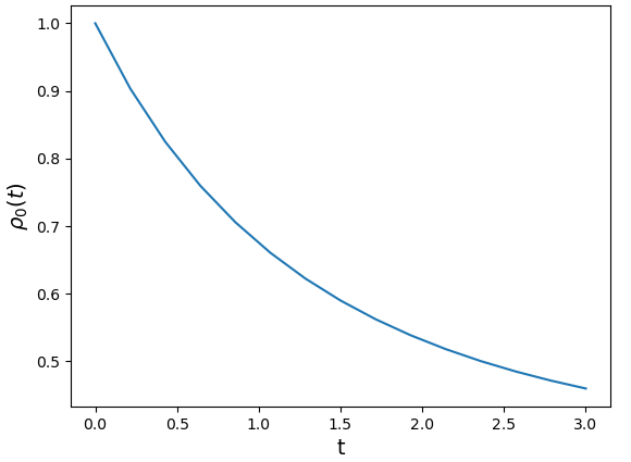
(a)

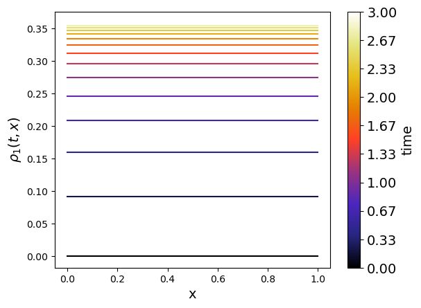
(b)

Figure 1: Solutions plots of the bdCDME generated with constant creation and degradation rates with $\lambda_{c}=\lambda_{d}=0.5$. a. The solution of $\rho_{0}(t)$ as a function of time. b. The solution of $\rho_{1}(t,x_{1})$ as a function of position and time.

and for $n\geq 1$

$$\rho_{n}(t,x_{1},...,x_{n}) =\exp\left\{-\lambda_{c}\frac{1-e^{-\lambda_{d}t}}{\lambda_{d}}\right\}\frac{1}{n!}\left(\lambda_{c}\frac{1-e^{-\lambda_{d}t}}{\lambda_{d}}\xi_{1}\right)^{\otimes n}(x_{1},...,x_{n})$$

$$=\exp\left\{-\lambda_{c}\frac{1-e^{-\lambda_{d}t}}{\lambda_{d}}\right\}\frac{1}{n!}\left(\lambda_{c}\frac{1-e^{-\lambda_{d}t}}{\lambda_{d}}\right)^{n}1(x_{1})\cdot\cdot\cdot 1(x_{n}).$$

This shows that for any $n\geq 1$ the function $\rho_{n}$ is constant in $x_{1},...,x_{n}$ with height given by the $n$-th component of the solution to the birth-death chemical master equation with stochastic rate constants $\lambda_{d}$ and $\lambda_{c}$ (compare with (1.6)).

Figure 1 shows the solutions for $\rho_{0}$ and $\rho_{1}$ as a function of time. Figure 1(a) shows the the exponential decay of the probability of having $0$ particles due to the constant creation of particles, and 1(b) shows the probability distribution of having $1$ particle is uniform in space for all times, as well as its convergence to the stationary distribution.

3.2 Dirac delta creation function at $x=0$

In this case we take $\lambda_{c}(x)=\lambda_{c}\delta_{0}(x)$, $x\in[0,1]$ for some positive constant $\lambda_{c}$, so the creation takes place only in the leftmost point of the interval while degradation happens uniformly. This way one yields

$$c_{j}=\int_{0}^{1}\lambda_{c}(x)\xi_{j}(x)dx=\int_{0}^{1}\lambda_{c}\delta_{0}(x)\xi_{j}(x)dx=\lambda_{c}\xi_{j}(0)=\lambda_{c},\quad\mbox{ for all $j\geq 1$}.$$

and formulas (3.2) and (3.3) now read

$$\rho_{0}(t)=\mathbb{P}(\mathcal{N}(t)=0)=\exp\left\{-\lambda_{c}\frac{1-e^{-\lambda_{d}t}}{\lambda_{d}}\right\},\quad t\geq 0,$$

(a)

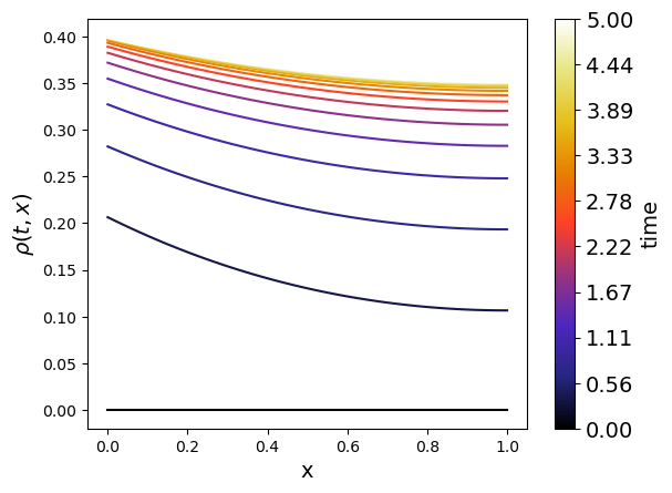
(b)

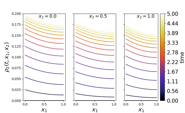
(c)

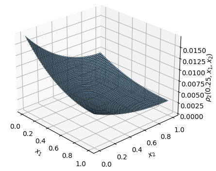
(d)

Figure 2: Solutions plots of the bdCDME generated with creation of particles at $x=0$ and constant degradation in the whole domain, namely with $\lambda_{c}(x)=0.5\delta_{0}(x)$ and $\lambda_{d}(x)=0.5$. The first 1000 terms of the sum in eq. 3.4 are considered. a. The solution of the $0$ particle density ($\rho_{0}(t)$) as a function of time. b. The solution of the $1$ particle density ($\rho_{1}(t,x_{1})$) for given position and time. c. The solution of the $2$ particle density ($\rho_{2}(t,x_{1},x_{2})$) with respect to $x_{1}$ and $t$ for three values of $x_{2}$. Time points as indicated in the color bar. d. The solution of the two particle density for fixed time, $\rho_{2}(t=0.25,x_{1},x_{2})$, as a function of $x_{1}$ and $x_{2}$.

and for $n\geq 1$

$$\rho_{n}(t,x_{1},...,x_{n}) =\exp\left\{-\lambda_{c}\frac{1-e^{-\lambda_{d}t}}{\lambda_{d}}\right\}\frac{1}{n!}\left(\sum_{j\geq 1}\lambda_{c}\frac{1-e^{-\alpha_{j}t}}{\alpha_{j}}\xi_{j}\right)^{\otimes n}(x_{1},...,x_{n})$$

$$=\exp\left\{-\lambda_{c}\frac{1-e^{-\lambda_{d}t}}{\lambda_{d}}\right\}\frac{\lambda_{c}^{n}}{n!}\left(\sum_{j\geq 1}\frac{1-e^{-\alpha_{j}t}}{\alpha_{j}}\xi_{j}\right)^{\otimes n}(x_{1},...,x_{n}).$$

We note that even though $\lambda_{c}(x)$ is a generalized function the series

$$\sum_{j\geq 1}c_{j}\frac{1-e^{-\alpha_{j}t}}{\alpha_{j}}\xi_{j}=\lambda_{c}\sum_{j\geq 1}\frac{1-e^{-\alpha_{j}t}}{\alpha_{j}}\xi_{j}$$ (3.4)

appearing above converges in $L^{2}([0,1])$.

In Figure 2 we plot solution of the bdCDME for this example. Figure 2(a) shows the exponential decay of the probability of having 0 particles due to the constant creation of particles. In contrast with Figure 1, in Figures 2(b) and 2(c), one can see the effect of the creation happening only at $x=0$ due to the peaks at the origin, while the highest peak is when $x_{2}=x_{1}=0$. With increasing time the peaks at the origin smooth out due to diffusion and probability being distributed through the different particle number densities. Similar to before, the curves converge to their stationary distribution as time increases. Lastly, Figure 2(d) shows the solution of the bdCDME for 2 particles as a surface on $x_{1},x_{2}$ axes, when time is fixed at $t=0.25$.

3.3 Dirac delta creation function at $x=1/2$

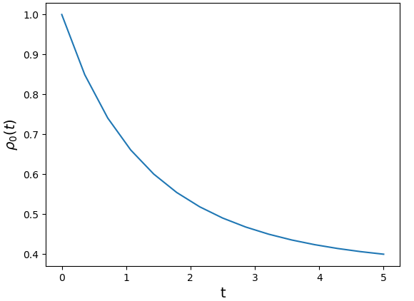
(a)

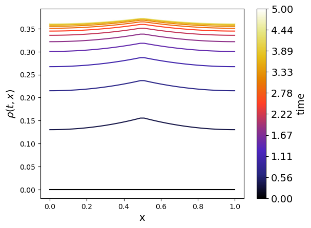
(b)

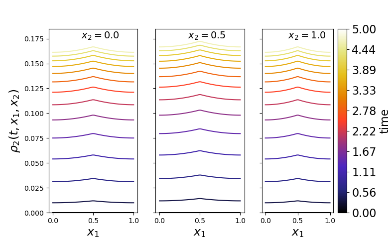
(c)

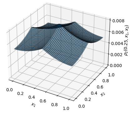
(d)

Figure 3: Solutions plots of the bdCDME generated with creation of particles at $x=0.5$ and constant degradation in the whole domain, namely $\lambda_{c}=0.5\delta_{1}/2(x)$ and $\lambda_{d}=0.5$. The first 1000 terms of the sum in eq. 3.4 are considered. a. The solution of the $0$ particle density ($\rho_{0}(t)$) as a function of time. b. The solution of the $1$ particle density ($\rho_{1}(t,x_{1})$) for given position and time. c. The solution of the $2$ particle density ($\rho_{2}(t,x_{1},x_{2})$) with respect to $x_{1}$ and $t$ for three values of $x_{2}$. Time points as indicated in the color bar. d. The solution of the two particle density for fixed time, $\rho_{2}(t=0.25,x_{1},x_{2})$, as a function of $x_{1}$ and $x_{2}$.

We now choose $\lambda_{c}(x)=\lambda_{c}\delta_{1/2}(x)$, $x\in[0,1]$ for some positive constant $\lambda_{c}$, so the creation takes place only on the middle of the interval and degradation happens uniformly. This way one obtains

$$c_{j}=\int_{0}^{1}\lambda_{c}(x)\xi_{j}(x)dx=\int_{0}^{1}\lambda_{c}\delta_{1/2}(x)\xi_{j}(x)dx=\lambda_{c}\xi_{j}(1/2)=\lambda_{c}\cos((j-1)\pi/2),\quad\mbox{ for all $j\geq 1$}.$$

Therefore, equations (3.2) and (3.3) take now the form

$$\rho_{0}(t)=\mathbb{P}(\mathcal{N}(t)=0)=\exp\left\{-\lambda_{c}\frac{1-e^{-\lambda_{d}t}}{\lambda_{d}}\right\},\quad t\geq 0,$$

and for $n\geq 1$

$$\rho_{n}(t,x_{1},...,x_{n}) =\exp\left\{-\lambda_{c}\frac{1-e^{-\lambda_{d}t}}{\lambda_{d}}\right\}\frac{1}{n!}\left(\sum_{j\geq 1}\lambda_{c}\cos((j-1)\pi/2)\frac{1-e^{-\alpha_{j}t}}{\alpha_{j}}\xi_{j}\right)^{\otimes n}(x_{1},...,x_{n})$$

$$=\exp\left\{-\lambda_{c}\frac{1-e^{-\lambda_{d}t}}{\lambda_{d}}\right\}\frac{\lambda_{c}^{n}}{n!}\left(\sum_{k\geq 1}(-1)^{k-1}\frac{1-e^{-\alpha_{2k-1}t}}{\alpha_{2k-1}}\xi_{2k-1}\right)^{\otimes n}(x_{1},...,x_{n}).$$

Figure 3 shows plots of the solution of the bdCDME for this example. Figure 3(a) shows the exponential decay of the probability of having $0$ particles due to the constant creation of particles. However, in conrast with figures 1 and 2, in this case, the effect of creation in the middle of the interval can be seen in the peaks in the Figures 3(b) and 3(c), while the highest peak is at $x_{1}=x_{2}=0.5$, as expected. Similar to the previous example the effect of the location of the creation of particles on the distribution becomes less important with increasing time due to diffusion. Once again, the curves converge to their stationary distribution. Lastly, Figure 3(d) plots the solution of bdCDME as a surface for 2 particle case at fixed time $t=0.25$, as a function of $x_{1}$ and $x_{2}$.

Acknowledgments

M.J.R acknowledges the support from Deutsche Forschungsgemeinschaft (DFG) (Grant No. RA 3601/1-1) and from the Dutch Institute for Emergent Phenomena (DIEP) cluster at the University of Amsterdam.

References

- [1] David F Anderson and Thomas G Kurtz. Stochastic analysis of biochemical systems, volume 1. Springer, 2015.
- [2] Steven S Andrews. Smoldyn: particle-based simulation with rule-based modeling, improved molecular interaction and a library interface. Bioinformatics, 33(5):710–717, 2017.
- [3] Wan Chen, Radek Erban, and S Jonathan Chapman. From Brownian dynamics to Markov chain: An ion channel example. SIAM Journal of Applied Mathematics, 74(1):208–235, 2014.
- [4] Mauricio J del Razo, Manuel Dibak, Christof Schütte, and Frank Noé. Multiscale molecular kinetics by coupling markov state models and reaction-diffusion dynamics. Journal of Chemical Physics, 155(12):124109, 2021.
- [5] Mauricio J. del Razo, Daniela Frömberg, Arthur V. Straube, Christof Schütte, Felix Höfling, and Stefanie Winkelmann. A probabilistic framework for particle-based reaction-diffusion dynamics using classical Fock space representations. Lett. Math. Phys., 112(3):Paper No. 49, 59, 2022.
- [6] Mauricio J del Razo, Hong Qian, and Frank Noé. Grand canonical diffusion-influenced reactions: A stochastic theory with applications to multiscale reaction-diffusion simulations. Journal of Chemical Physics, 149(4):044102, 2018.
- [7] Mauricio J del Razo, Stefanie Winkelmann, Rupert Klein, and Felix Höfling. Chemical diffusion master equation: Formulations of reaction–diffusion processes on the molecular level. J. Math. Phys., 64(1):013304, 2023.
- [8] Peter Deuflhard, Wilhelm Huisinga, Tobias Jahnke, and Michael Wulkow. Adaptive discrete galerkin methods applied to the chemical master equation. SIAM Journal on Scientific Computing, 30(6):2990–3011, 2008.
- [9] Manuel Dibak, Mauricio J del Razo, David De Sancho, Christof Schütte, and Frank Noé. Msm/rd: Coupling markov state models of molecular kinetics with reaction-diffusion simulations. Journal of Chemical Physics, 148(21):214107, 2018.
- [10] Masao Doi. Second quantization representation for classical many-particle system. Journal of Physics A: Mathematical and General, 9(9):1465, 1976.
- [11] Stefan Engblom. Spectral approximation of solutions to the chemical master equation. Journal of computational and applied mathematics, 229(1):208–221, 2009.
- [12] Mark B Flegg, S Jonathan Chapman, and Radek Erban. The two-regime method for optimizing stochastic reaction–diffusion simulations. Journal of the Royal Society Interface, 9(70):859–868, 2012.
- [13] Daniel T Gillespie. Exact stochastic simulation of coupled chemical reactions. The journal of physical chemistry, 81(25):2340–2361, 1977.
- [14] Ankit Gupta, Christoph Schwab, and Mustafa Khammash. Deepcme: A deep learning framework for computing solution statistics of the chemical master equation. PLoS computational biology, 17(12):e1009623, 2021.
- [15] Moritz Hoffmann, Christoph Fröhner, and Frank Noé. Readdy 2: Fast and flexible software framework for interacting-particle reaction dynamics. PLoS computational biology, 15(2):e1006830, 2019.
- [16] Tobias Jahnke and Wilhelm Huisinga. Solving the chemical master equation for monomolecular reaction systems analytically. Journal of mathematical biology, 54:1–26, 2007.
- [17] Qingchao Jiang, Xiaoming Fu, Shifu Yan, Runlai Li, Wenli Du, Zhixing Cao, Feng Qian, and Ramon Grima. Neural network aided approximation and parameter inference of non-markovian models of gene expression. Nature communications, 12(1):1–12, 2021.
- [18] Ioannis Karatzas and Steven E. Shreve. Brownian motion and stochastic calculus, volume 113 of Graduate Texts in Mathematics. Springer-Verlag, New York, second edition, 1991.
- [19] Margarita Kostré, Christof Schütte, Frank Noé, and Mauricio J del Razo. Coupling particle-based reaction-diffusion simulations with reservoirs mediated by reaction-diffusion pdes. SIAM Multiscale Modeling & Simulation, 19(4):1659–1683, 2021.
- [20] Alberto Lanconelli. Using Malliavin calculus to solve a chemical diffusion master equation. arXiv:2203.14676, 2022.
- [21] Donald A. McQuarrie. Stochastic approach to chemical kinetics. J. Appl. Probability, 4:413–478, 1967.
- [22] Brian Munsky and Mustafa Khammash. The finite state projection algorithm for the solution of the chemical master equation. The Journal of chemical physics, 124(4):044104, 2006.
- [23] Hong Qian and Lisa M Bishop. The chemical master equation approach to nonequilibrium steady-state of open biochemical systems: Linear single-molecule etheornzyme kinetics and nonlinear biochemical reaction networks. Int. J. Mol. Sci., 11(9):3472–3500, 2010.
- [24] Hong Qian and Hao Ge. Stochastic Chemical Reaction Systems in Biology. Springer, 2021.
- [25] David Schnoerr, Guido Sanguinetti, and Ramon Grima. Approximation and inference methods for stochastic biochemical kinetics—a tutorial review. Journal of Physics A: Mathematical and Theoretical, 50(9):093001, 2017.
- [26] Frank Schweitzer and J Doyne Farmer. Brownian agents and active particles: collective dynamics in the natural and social sciences, volume 1. Springer, 2003.
- [27] Cameron A Smith and Christian A Yates. Spatially extended hybrid methods: a review. Journal of the Royal Society Interface, 15(139):20170931, 2018.