Structured Bayesian Compression for Deep Neural Networks Based on The Turbo-VBI Approach

Abstract

With the growth of neural network size, model compression has attracted increasing interest in recent research. As one of the most common techniques, pruning has been studied for a long time. By exploiting the structured sparsity of the neural network, existing methods can prune neurons instead of individual weights. However, in most existing pruning methods, surviving neurons are randomly connected in the neural network without any structure, and the non-zero weights within each neuron are also randomly distributed. Such irregular sparse structure can cause very high control overhead and irregular memory access for the hardware and even increase the neural network computational complexity. In this paper, we propose a three-layer hierarchical prior to promote a more regular sparse structure during pruning. The proposed three-layer hierarchical prior can achieve per-neuron weight-level structured sparsity and neuron-level structured sparsity. We derive an efficient Turbo-variational Bayesian inferencing (Turbo-VBI) algorithm to solve the resulting model compression problem with the proposed prior. The proposed Turbo-VBI algorithm has low complexity and can support more general priors than existing model compression algorithms. Simulation results show that our proposed algorithm can promote a more regular structure in the pruned neural networks while achieving even better performance in terms of compression rate and inferencing accuracy compared with the baselines.

I Introduction

Deep neural networks (DNNs) have been extremely successful in a wide range of applications. However, to achieve good performance, state-of-the-art DNNs tend to have huge numbers of parameters. Deployment and transmission of such big models pose significant challenges for computation, memory and communication. This is particularly important for edge devices, which have very restricted resources. For the above reasons, model compression has become a hot topic in deep learning.

A variety of research focused on model compression exists. In [1]-[3], the weight pruning approaches are adopted to reduce the complexity of DNN inferencing. In [1], the threshold is set to be the weight importance, which is measured by introducing an auxiliary importance variable for each weight. With the auxiliary variables, the pruning can be performed in one shot and before the formal training. In [2] and [3], Hessian matrix of the weights are used as a criterion to perform pruning. These aforementioned approaches, however, cannot proactively force some of the less important weights to have small values and hence the approaches just passively prune small weights. In [4]-[13], systematic approaches of model compression using optimization of regularized loss functions are adopted. In [11], an $\ell_{2}$-norm based regularizer is applied to the weights of a DNN and the weights that are close to zero are pruned. In [4], an $\ell_{0}$-norm regularizer, which forces the weights to be exactly zero, is proposed. The $\ell_{0}$-norm regularization is proved to be more efficient to enforce sparsity in the weights but the training problem is notoriously difficult to solve due to the discontinuous nature of the $\ell_{0}$-norm. In these works, the regularization only promotes sparsity in the weights. Yet, sparsity in the weights is not equivalent to sparsity in the neurons. In [9], polarization regularization is proposed, which can push a proportion of weights to zero and others to values larger than zero. Then, all the weights connected to the same neuron are assigned with a common polarization regularizer, such that some neurons can be entirely pruned and some can be pushed to values larger than zero. In this way, the remaining weights do not have to be pushed to small values and hence can improve the expressing ability of the network. In [5], the authors use a group Lasso regularizer to remove entire filters in CNNs and show that their proposed group sparse regularization can even increase the accuracy of a ResNet. However, the resulting neurons are randomly connected in the neural network and the resulting datapath of the pruned neural network is quite irregular, making it difficult to implement in hardware [5, 6].

In addition to the aforementioned deterministic regularization approaches, we can also impose sparsity in the weights of the neural network using Bayesian approaches. In [14], weight pruning and quantization are realized at the same time by assigning a set of quantizing gates to the weight value. A prior is further designed to force the quantizing gates to “close”, such that the weights are forced to zero and the non-zero weights are forced to a low bit precision. By designing an appropriate prior distribution for the weights, one can enforce more refined structures in the weight vector. In [15], a simple sparse prior is proposed to promote weight-level sparsity, and variational Bayesian inference (VBI) is adopted to solve the model compression problem. In [16], group sparsity is investigated from a Bayesian perspective. A two-layer hierarchical sparse prior is proposed where the weights follow Gaussian distributions and all the output weights of a neuron share the same prior variance. Thus, the output weights of a neuron can be pruned at the same time and neuron-level sparsity is achieved.

In this paper, we consider model compression of DNNs from a Bayesian perspective. Despite various existing works on model compression, there are still several technical issues to be addressed.

• Structured datapath in the pruned neural network: In deterministic regularization approaches, we can achieve group sparsity in a weight matrix. For example, under $\ell_{2,1}$-norm regularization [5, 7], some rows can be zeroed out in the weight matrix after pruning and this results in neuron-level sparsity. However, surviving neurons are randomly connected in the neural network without any structure. Moreover, the non-zero weights within each neuron are also randomly distributed. In the existing Bayesian approaches, both the single-layer priors in [15] and the two-layer hierarchical priors in [16] also cannot promote structured neuron connectivity in the pruned neural network. As such, the random and irregular neuron connectivity in the datapath of the DNN poses challenges in the hardware implementation.

• Efficiency of weight pruning: With existing model compression approaches, the compressed model can still be too large for efficient implementation on mobile devices. Moreover, the existing Bayesian model compression approaches tend to have high complexity and low robustness with respect to different data sets, as they typically adopt Monte Carlo sampling in solving the optimizing problem [15, 16]. Thus, a more efficient model compression solution that can achieve a higher compression rate and lower complexity is required.

To overcome the above challenges, we propose a three-layer hierarchical sparse prior that can exploit structured weight-level and neuron-level sparsity during training. To handle the hierarchical sparse prior, we propose a Turbo-VBI [17] algorithm to solve the Bayesian optimization problem in the model compression. The main contributions are summarized below.

• Three-layer Hierarchical Prior for Structured Weight-level and Neuron-level Sparsity: The design of an appropriate prior distribution in the weight matrix is critical to achieve more refined structures in the weights and neurons. To exploit more structured weight-level and neuron-level sparsity, we propose a three-layer hierarchical prior which embraces both of the traditional two-layer hierarchical prior [16] and support-based prior [18]. The proposed three-layer hierarchical prior has the following advantages compared with existing sparse priors in Bayesian model compression: 1) It promotes advanced weight-level structured sparsity as well as neuron-level structured sparsity, as illustrated in Fig. 1c. Unlike existing sparse priors, our proposed prior not only prunes the neurons, but also promotes regular structures in the unpruned neurons as well as the weights of a neuron. Thus, it can achieve more regular structure in the overall neural network. 2) It is flexible to promote different sparse structures. The group size as well as the average gap between two groups can be adjusted via tuning the hyper parameters. 3) It is optimizing-friendly. It allows the application of low complexity training algorithms.

• Turbo-VBI Algorithm for Bayesian Model Compression: Based on the 3-layer hierarchical prior, the model training and compression is formulated as a Bayesian inference problem. We propose a low complexity Turbo-VBI algorithm with some novel extensions compared to existing approaches: 1) It can support more general priors. Existing Bayesian compression methods [15, 16] cannot handle the three-layer hierarchical prior due to the extra layer in the prior. 2) It has higher robustness and lower complexity compared with existing Bayesian compression methods. Existing Bayesian compression methods use Monte Carlo sampling to approximate the log-likelihood term in the objective function, which has low robustness and high complexity [19]. To overcome this drawback, we propose a deterministic approximation for the log-likelihood term.

• Superior Model Compression Performance: The proposed solution can achieve a highly compressed neural network compared to the state-of-the-art baselines and achieves a similar inferencing performance. Therefore, the proposed solution can substantially reduce the computational complexity in the inferencing of the neural network and the resulting pruned neural networks are hardware friendly. Consequently, it can fully unleash the potential of AI applications over mobile devices.

The rest of the paper is organized as follows. In Section II, the existing structures and the desired structure in the weight matrix are elaborated. The three-layer hierarchical prior for the desired structure is also introduced. In Section III, the model compression problem is formulated. In Section IV, the Turbo-VBI algorithm for model compression under the three-layer hierarchical prior is presented. In Section V and Section VI, numerical experiments and conclusions, respectively, are provided.

II Structures in The Weight Matrix

Model compression is realized by enforcing sparsity in the weight matrix. We first review the main existing structured sparsity of the weight matrix in the literature. Based on this, we elaborate the desired structures in the weight matrix that are not yet considered. Finally, we propose a 3-layer hierarchical prior model to enforce such a desired structure in the weight matrix.

II-A Review of Existing Sparse Structured Weight Matrix

(a) Random sparsity structure.

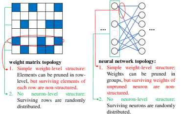
(b) Group sparsity structure.

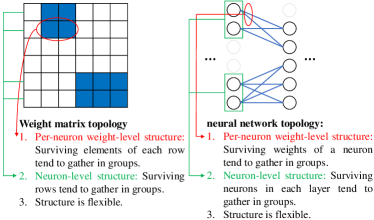
(c) Proposed multi-level structure.

Figure 1: Comparison of different structures in the weight matrix of a fully connected layer with 6 input neurons and 6 output neurons. Each row denotes the weights connected to one input neuron.

There are two major existing sparse structures in the weight matrix, namely random sparsity and group sparsity. We focus on a fully connected layer to elaborate these two sparse structures.

1) Random Sparsity in the Weight Matrix: In random sparsity, the weights are pruned individually. $\ell_{1}$-norm regularization and one-layer prior [15] are often adopted to regularize individual weights. Such regularization is simple and optimization-friendly; however, both resulting weights and neurons are completely randomly connected since there is no extra constraint on the pruned weights. In the weight matrix, this means that the elements are set to zero without any structure, which results in the remaining elements also having no specific structures. When translated into neural network topology, this means that the surviving weights and neurons are randomly connected, as illustrated in Fig. 1a. Because of the random connections in the pruned network, such a structure is not friendly to practical applications such as storage, computation and transmission [5, 20].

2) Group Sparsity in the Weight Matrix: In group sparsity, the weights are pruned in groups. Particularly, in fully connected layers, a group is often defined as the outgoing weights of a neuron to promote neuron-level sparsity. To promote group sparsity, sparse group Lasso regularization [7, 21] and two-layer priors are proposed. Generally, such regularization often has two folds: one regularizer for group pruning and one regularizer for individual weight pruning. Thus, the weights can not only be pruned in groups, but can also be pruned individually in case the group cannot be totally removed. However, when a neuron cannot be totally pruned, the weights connected to it are randomly pruned, and the neurons are also pruned in random. In Fig. 1b, we illustrate an example of group sparsity. In the weight matrix, the non-zero elements in a row are randomly distributed and the non-zero rows are also randomly distributed. When translated into neural network topology, this means the unpruned weights connected to a neuron are randomly distributed, and in each layer, the surviving neurons are also randomly distributed. Thus, group sparsity is still not fully structured.

On the other hand, recent research has pointed out that the irregular connections in the neural network can bring various disadvantages in reducing the computational complexity or inferencing time [20], [22]-[25]. As discussed above, existing sparsity structures are not regular enough, and the drawbacks of such irregular structures are listed as follows.

1. Low decoding and computing parallelism: Sparse weight matrix are usually stored in a sparse format on the hardware, e.g., compressed sparse row (CSR), compressed sparse column (CSC), coordinate format (COO). However, as illustrated in Fig. 2 (a), when decoding from the sparse format, the number of decoding steps for each row (column) can vastly differ due to the irregular structure. This can greatly harm the decoding parallelism [23]. Moreover, the irregular structure also hampers the parallel computation such as matrix tiling [24, 20], as illustrated in Fig. 2 (b).

2. Inefficient pruning of neurons: As illustrated in Fig. 2 (c), the unstructured surviving weights from the previous layer tend to activate random neurons in the next layer, which is not efficient in pruning the neurons in the next layer. This may lead to inefficiency in reducing the floating point operations (FLOPs) of the pruned neural network.

3. Large storage burden: Since the surviving weights of existing model compression methods are unstructured, the exact location for each surviving weight has to be recorded. This leads to a huge storage overhead, which can be even greater than storing the dense matrix [24, 20]. The huge storage overhead can also affect the inferencing time by increasing the memory access and decoding time.

II-B Multi-level Structures in the Weight Matrix

Based on the above discussion, a multi-level structured sparse neural network should meet the following three criteria: 1) Per-neuron weight-level structured sparsity: The surviving weights connected to a neuron should exhibit a regular structure rather than be randomly distributed as in traditional group sparsity. In a weight matrix, this means the non-zero elements of each row should follow some regular structure. 2) Neuron-level structured sparsity: The surviving neurons of each layer should also have some regular structures. In a weight matrix, this means that the non-zero rows should also follow some structure. 3) Flexibility: The structure of the resulting weight matrix should be sufficiently flexible so that we can achieve a trade off between model complexity and predicting accuracy in different scenarios. Fig. 1c illustrates an example of a desired structure in the weight matrix. In each row, the significant values tend to gather in groups. When translated into neural network topology, this enables the advanced weight-level structure: The surviving weights of each neuron tend to gather in groups. In each column, the significant values also tend to gather in groups. When translated into neural network topology, this enables the neuron-level structure: The surviving neurons in each layer tend to gather in groups. Moreover, the group size in each row and column can be tuned to achieve a trade off between model complexity and predicting accuracy. Such proposed multi-level structures enable the datapath to exploit the compression to simplify the computation with very small control overheads. Specifically, the advantages of our proposed multi-level structure are listed as follows.

1. High decoding and computing parallelism: As illustrated in Fig. 2 (a), with the blocked structure, the decoding can be performed in block wise such that all the weights in the same block can be decoded simultaneously. Moreover, the regular structure can bring more parallelism in computation. For example, more efficient matrix tiling can be applied, where the zero blocks can be skipped during matrix multiplication, as illustrated in Fig. 2 (b). Also, the kernels can be compressed into smaller size, such that the inputs corresponding to the zero weights can be skipped [20].

2. Efficient neuron pruning: As illustrated in Fig. 2 (c), the structured surviving weights from the previous layer can lead to a structured and compact neuron activation in the next layer, which is beneficial for more efficient neuron pruning.

3. More efficient storage: With the blocked structure, we can simply record the location and size for each block rather than recording the exact location for each weight. For a weight matrix with average cluster size of $m\times m$ and number of clusters $P$, the coding gain over traditional COO format is $\mathcal{O}\left(Pm^{2}\right)$.

In this paper, we focus on promoting a multi-level group structure in model compression. In our proposed structure, the surviving weights connected to a neuron tend to gather in groups and the surviving neurons also tend to gather in groups. Additionally, the group size is tunable so that our proposed structure is flexible.

Figure 2: (a) Illustration of decoding parallelism. In existing sparse structures, the decoding step for each row can be vastly different because of the irregular structure. In our proposed structure, each block can be decoded simultaneously because each block can be coded as a whole. (b) Illustration of computing parallelism. In existing sparse structures, the matrix-matrix multiplication has to be performed element-wise because each non-zero weight is individually encoded. The processor has to fetch individual weights and multiply them to individual input elements to get the individual output element (green square). In our proposed structure, parallel techinics for dense matrix such as matrix tiling can be applied. Moreover, due to the clustered structure, the zero block (gray block) can be skipped during computing the output (green block). (c) Illustration of efficient neuron pruning. In existing sparse structures, the surviving weights of each neuron are randomly connected to the neurons in the next layer, which will randomly activate neurons in the next layer. In our proposed structure, the surviving weights of each neuron tend to activate the same neurons in the next layer, which can lead to a structured and compact neuron activation in the next layer.

II-C Three-Layer Hierarchical Prior Model

The probability model of the sparse prior provides the foundation of specific sparse structures. As previously mentioned, existing sparse priors for model compression cannot promote the multi-level structure in the weight matrix. To capture the multi-level structured sparsity, we propose a three-layer hierarchical prior by combining the two-layer prior and the support based prior [18].

Let $w$ denote a weight in the neural network. For each weight $w$, we introduce a support $s\in\left\{0,1\right\}$ to indicate whether the weight $w$ is active $\left(s=1\right)$ or inactive $\left(s=0\right)$. Specifically, let $\rho$ denote the precision for the weight $w$. That is, $1/\rho$ is the variance of $w$. When $s=0$, the distribution of $\rho$ is chosen to satisfy $\mathbb{E}\left[\rho\right]\gg 1$, so that the variance of the corresponding weight $w$ is very small. When $s=1$, the distribution of $\rho$ is chosen to satisfy $\mathbb{E}\left[\rho\right]=\mathcal{O}\left(1\right)$, so that $w$ has some probability to take significant values. Then, the three-layer hierarchical prior (joint distribution of $\mathbf{w},\boldsymbol{\rho},\mathbf{s}$) is given by

$$p\left(\mathbf{w},\boldsymbol{\rho},\mathbf{s}\right)=p\left(\mathbf{s}\right)p\left(\boldsymbol{\rho}|\mathbf{s}\right)p\left(\mathbf{w}|\boldsymbol{\rho}\right),$$ (1)

where $\mathbf{w}$ denotes all the weights in the neural network, $\boldsymbol{\rho}$ denotes the corresponding precisions, and $\mathbf{s}$ denotes the corresponding supports. The distribution of each layer is elaborated below.

Probability Model for $p\left(\mathbf{s}\right)$: $p\left(\mathbf{s}\right)$ can be decomposed into each layer by $p\left(\mathbf{s}\right)=\prod_{l=1}^{L}p\left(\mathbf{s}_{l}\right)$, where $L$ is the total layer number of the neural network and $\mathbf{s}_{l}$ denotes the supports of the weights in the $l$-th layer. Now we focus on the $l$-th layer. Suppose the dimension of the weight matrix is $K\times M$, i.e., the layer has $K$ input neurons and $M$ output neurons. The distribution $p\left(\mathbf{s}_{l}\right)$ of the supports is used to capture the multi-level structure in this layer. Since we focus on a specific layer now, we use $p\left(\mathbf{s}\right)$ to replace $p\left(\mathbf{s}_{l}\right)$ in the following discussion for notation simplicity. In order to promote the aforementioned multi-level structure, the active elements in each row of the weight matrix should gather in clusters and the active elements in each column of the weight matrix should also gather in clusters. Such a block structure can be achieved by modeling the support matrix as a Markov random field (MRF). Specifically, each row of the support matrix is modeled by a Markov chain as

$$p\left(\mathbf{s}_{row}\right)=p\left(s_{row,1}\right)\prod_{m=1}^{M}p\left(s_{row,m+1}|s_{row,m}\right),$$ (2)

where $\mathbf{s}_{row}$ denotes the row vector of the support matrix, and $s_{row,m}$ denotes the $m$-th element in $\mathbf{s}_{row}$. The transition probability is given by $p\left(s_{row,m+1}=1|s_{row,m}=0\right)=p_{01}^{row}$ and $p\left(s_{row,m+1}=0|s_{row,m}=1\right)=p_{10}^{row}$. Generally, a smaller $p_{01}^{row}$ leads to a larger average gap between two clusters, and a smaller $p_{10}^{row}$ leads to a larger average cluster size. Similarly, each column of the support matrix is also modeled by a Markov chain as

$$p\left(\mathbf{s}_{col}\right)=p\left(s_{col,1}\right)\prod_{k=1}^{K}p\left(s_{col,k+1}|s_{col,k}\right),$$ (3)

where $\mathbf{s}_{col}$ denotes the column vector of the support matrix and $s_{col,k}$ denotes the $n$-th element in $\mathbf{s}_{col}$. The transition probability is given by $p\left(s_{col,k+1}=1|s_{col,k}=0\right)=p_{01}^{col}$ and $p\left(s_{col,k+1}=0|s_{col,k}=1\right)=p_{10}^{col}$. Such an MRF model is also known as a 2D Ising model. An illustration of the MRF prior is given in Fig. 3. Note that $p\left(\mathbf{s}\right)$ can also be modeled with other types of priors, such as Markov tree prior and hidden Markov prior, to promote other structures.

Figure 3: Illustration of the support prior for a $6\times 6$ weight matrix.

Probability Model for $p\left(\boldsymbol{\rho}|\mathbf{s}\right)$: The conditional probability $p\left(\boldsymbol{\rho}|\mathbf{s}\right)$ is given by

$$p\left(\boldsymbol{\rho}|\mathbf{s}\right)=\prod_{n=1}^{N}\left(\Gamma\left(\rho_{n};a_{n},b_{n}\right)\right)^{s_{n}}\left(\Gamma\left(\rho_{n};\overline{a}_{n},\overline{b}_{n}\right)\right)^{1-s_{n}},$$ (4)

where $N$ is the total number of weights in the neural network. $\rho_{n}$ takes two different Gamma distributions according to the value of $s_{n}$. When $s_{n}=1$, the corresponding weight $w_{n}$ is active. In this case, the shape parameter $a_{n}$ and rate parameter $b_{n}$ should satisfy that $\frac{a_{n}}{b_{n}}=\mathbb{E}\left[\rho_{n}\right]=\mathcal{O}\left(1\right)$ such that the variance of $w_{n}$ is $\mathcal{O}\left(1\right)$. When $s_{n}=0$, the corresponding weight $w_{n}$ is inactive. In this case, the shape parameter $\overline{a}_{n}$ and rate parameter $\overline{b}_{n}$ should satisfy that $\frac{\overline{a}_{n}}{\overline{b}_{n}}=\mathbb{E}\left[\rho_{n}\right]\gg 1$ such that the variance of $w_{n}$ is very close to zero. The motivation for choosing Gamma distribution is that Gamma distribution is conjugate to Gaussian distribution. Thus, it can leads to a closed form solution in Bayesian inference [17].

Probability Model for $p\left(\mathbf{w}|\boldsymbol{\rho}\right)$: The conditional probability $p\left(\mathbf{w}|\boldsymbol{\rho}\right)$ is given by

$$p\left(\mathbf{w}|\boldsymbol{\rho}\right)=\prod_{n=1}^{N}p\left(w_{n}|\rho_{n}\right),$$ (5)

where $p\left(w_{n}|\rho_{n}\right)$ is assumed to be a Gaussian distribution:

$$p\left(w_{n}|\rho_{n}\right)=\mathcal{N}\left(w_{n}|0,\frac{1}{\rho_{n}}\right).$$ (6)

Although the choice of $p\left(w_{n}|\rho_{n}\right)$ is not restricted to Gaussian distribution [16], the motivation for choosing Gaussian is still reasonable. First, according to existing simulations, the compression performance is not so sensitive to the distribution type of $p\left(w_{n}|\rho_{n}\right)$ [16, 15]. Moreover, assuming $p\left(w_{n}|\rho_{n}\right)$ to be a Gaussian distribution also contributes to easier optimization in Bayesian inference, as shown in Section IV.

Remark 1. (Comparison with existing sparse priors) One of the main differences between our work and the existing works [15, 16] is the design of the prior. Because of the MRF support layer, our proposed three-layer prior is more general and can capture more regular structures such as the desired multi-level structure. Such a multi-level structure in the weight matrix cannot be modeled by the existing priors in [15] and [16] but our proposed prior can easily support the sparse structures in them. In our work, if the prior $p\left(\mathbf{w},\boldsymbol{\rho},\mathbf{s}\right)$ reduces to one layer $p\left(\mathbf{w}\right)$ and takes a Laplace distribution, it is equivalent to a Lasso regularization. In this way, random sparsity can be realized. If the prior $p\left(\mathbf{w},\boldsymbol{\rho},\mathbf{s}\right)$ reduces to one layer $p\left(\mathbf{w}\right)$ and takes an improper log-scale uniform distribution, it is exactly the problem of variational dropout [15]. In this way, random sparsity can be realized. If the prior $p\left(\mathbf{w},\boldsymbol{\rho},\mathbf{s}\right)$ reduces to a two-layer $p\left(\mathbf{w}|\boldsymbol{\rho}\right)$, and takes the group improper log-uniform distribution or the group horseshoe distribution, it is exactly the problem in [16]. In this way, group sparsity can be realized. Moreover, since our proposed prior is more complicated, it also leads to a different algorithm design in Section IV.

III Bayesian Model Compression Formulation

Bayesian model compression handles the model compression problem from a Bayesian perspective. In Bayesian model compression, the weights follow a prior distribution, and our primary goal is to find the posterior distribution conditioned on the dataset. In the following, we elaborate on the neural network model and the Bayesian training of the DNN.

III-A Neural Network Model

We first introduce the neural network model. Let $\mathcal{D}=\left\{\left(x_{1},y_{1}\right),\left(x_{2},y_{2}\right),...,\left(x_{D},y_{D}\right)\right\}$ denote the dataset, which contains $D$ pairs of training input $\left(x_{d}\right)$ and training output $\left(y_{d}\right)$. Let $NN\left(x,\mathbf{w}\right)$ denote the output of the neural network with input $x$ and weights $\mathbf{w}$, where $NN\left(\cdot\right)$ is the neural network function. Note that $NN\left(x,\mathbf{w}\right)$ is a generic neural network model, which can embrace various commonly used structures, some examples are listed as follows.

• Multi-Layer Perceptron (MLP): MLP is a representative class of feedforward neural network, which consists of an input layer, output layer and hidden layers. As illustrated in Fig. 4a, we can use $NN\left(x,\mathbf{w}\right)$ to represent the feedforward calculation in an MLP.

• Convolutional Neural Network (CNN): A CNN consists of convolutional kernels and dense layers. As illustrated in Fig. 4b, we can use $NN\left(x,\mathbf{w}\right)$ to represent the complicated calculation in a CNN.

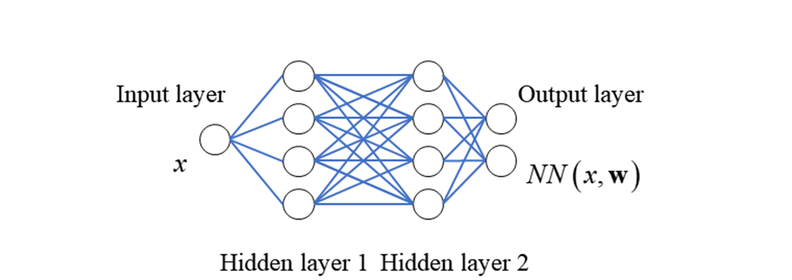
(a) Illustration of $NN\left(x,\mathbf{w}\right)$ in MLP.

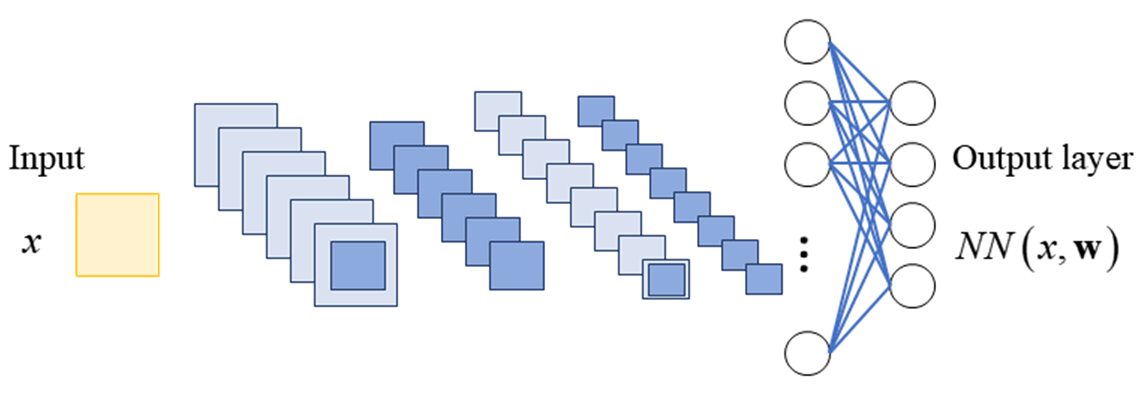
(b) Illustration of $NN\left(x,\mathbf{w}\right)$ in CNN.

Figure 4: Illustration of $NN\left(x,\mathbf{w}\right)$ in different neural networks.

Since the data points from the training set are generally assumed to be independent, we can use the following stochastic model to describe the observations from a general neural network:

$$\mathbf{y}\sim p\left(\mathcal{D}|\mathbf{w}\right)=\prod_{d=1}^{D}p\left(y_{d}|x_{d},\mathbf{w}\right),$$ (7)

where the likelihood $p\left(y_{d}|x_{d},\mathbf{w}\right)$ can be different for regression and classification tasks [26]. In regression tasks, it can be modeled as a Gaussian distribution:

$$p\left(y_{d}|x_{d},\mathbf{w}\right)=\mathcal{N}\left(NN\left(x_{d},\mathbf{w}\right),\sigma_{d}^{2}\right),$$ (8)

where $\sigma_{d}^{2}$ is the noise variance in training data, while in classification tasks, it can be modeled as

$$p\left(y_{d}|x_{d},\mathbf{w}\right)=\exp\left(-G\left(y_{d}|x_{d},\mathbf{w}\right)\right),$$ (9)

where $G\left(y_{d}|x_{d},\mathbf{w}\right)$ is the cross-entropy error function.

III-B Bayesian Training of DNNs

Bayesian training of a DNN is actually calculating the posterior distribution $p\left(\mathbf{w},\boldsymbol{\rho},\mathbf{s}|\mathcal{D}\right)$ based on the prior distribution $p\left(\mathbf{w},\boldsymbol{\rho},\mathbf{s}\right)$ and the neural network stochastic model (7). In our research, after we obtain the posterior $p\left(\mathbf{w},\boldsymbol{\rho},\mathbf{s}|\mathcal{D}\right)$, we use the maximum a posteriori (MAP) estimate of $\mathbf{w},\boldsymbol{\rho}$ and $\mathbf{s}$ as a deterministic estimate of the weights, precision and support, respectively:

$$\left(\mathbf{w},\boldsymbol{\rho},\mathbf{s}\right)^{*}=\arg\max_{\mathbf{w},\boldsymbol{\rho},\mathbf{s}}p\left(\mathbf{w},\boldsymbol{\rho},\mathbf{s}|\mathcal{D}\right).$$ (10)

According to Bayesian rule, the posterior distribution of $\mathbf{w},\boldsymbol{\rho}$ and $\mathbf{s}$ can be derived as

$$p\left(\mathbf{w},\boldsymbol{\rho},\mathbf{s}|\mathcal{D}\right)=\frac{p\left(\mathcal{D}|\mathbf{w},\boldsymbol{\rho},\mathbf{s}\right)p\left(\mathbf{w},\boldsymbol{\rho},\mathbf{s}\right)}{p\left(\mathcal{D}\right)},$$ (11)

where $p\left(\mathcal{D}|\mathbf{w},\boldsymbol{\rho},\mathbf{s}\right)$ is the likelihood term. Based on (7) and (8), it is given by:

$$p\left(\mathcal{D}|\mathbf{w},\boldsymbol{\rho},\mathbf{s}\right)=\prod_{d=1}^{D}p\left(y_{d}|x_{d},\mathbf{w},\boldsymbol{\rho},\mathbf{s}\right),$$ (12)

$$p\left(y_{d}|x_{d},\mathbf{w},\boldsymbol{\rho},\mathbf{s}\right)=\mathcal{N}\left(NN\left(x_{d},\mathbf{w},\boldsymbol{\rho},\mathbf{s}\right),\sigma_{d}^{2}\right).$$ (13)

Equation (11) mainly contains two terms: 1) Likelihood $p\left(\mathcal{D}|\mathbf{w},\boldsymbol{\rho},\mathbf{s}\right)$, which is related to the expression of dataset. 2) Prior $p\left(\mathbf{w},\boldsymbol{\rho},\mathbf{s}\right)$, which is related to the sparse structure we want to promote. Intuitively, by Bayesian training of the DNN, we are actually simultaneously 1) tuning the weights to express the dataset and 2) tuning the weights to promote the structure captured in the prior.

However, directly computing the posterior according to (11) involves several challenges, summarized as follows.

• Intractable multidimensional integral: The calculation of the exact posterior $p\left(\mathbf{w},\boldsymbol{\rho},\mathbf{s}|\mathcal{D}\right)$ involves calculating the so-called evidence term $p\left(\mathcal{D}\right)$. The calculation of $p\left(\mathcal{D}\right)=\sum_{\mathbf{s}}\int\int p\left(\mathcal{D}|\mathbf{w},\boldsymbol{\rho},\mathbf{s}\right)p\left(\mathbf{w},\boldsymbol{\rho},\mathbf{s}\right)d\mathbf{w}d\boldsymbol{\rho}$ is usually intractable as the likelihood term can be very complicated [26].

• Complicated prior term: Since the prior term $p\left(\mathbf{w},\boldsymbol{\rho},\mathbf{s}\right)$ contains an extra support layer $p\left(\mathbf{s}\right)$, the KL-divergence between the approximate distribution and the posterior distribution is difficult to calculate or approximate. Traditional VBI method cannot be directly applied to achieve an approximate posterior distribution.

In the next section, we propose a Turbo-VBI based model compression method, which approximately calculates the marginal posterior distribution of $\mathbf{w},\boldsymbol{\rho}$ and $\mathbf{s}$.

IV Turbo-VBI Algorithm for Model Compression

To handle the aforementioned two challenges, we propose a Turbo-VBI [17] based model compression algorithm. The basic idea of the proposed Turbo-VBI algorithm is to approximate the intractable posterior $p\left(\mathbf{w},\boldsymbol{\rho},\mathbf{s}|\mathcal{D}\right)$ with a variational distribution $q\left(\mathbf{w},\boldsymbol{\rho},\mathbf{s}\right)$. The factor graph of the joint distribution $p\left(\mathbf{w},\boldsymbol{\rho},\mathbf{s},\mathcal{D}\right)$ is illustrated in Fig. 5, where the variable nodes are denoted by white circles and the factor nodes are denoted by black squares. Specifically, the factor graph is derived based on the factorization

$$p\left(\mathbf{w},\boldsymbol{\rho},\mathbf{s},\mathcal{D}\right)=p\left(\mathcal{D}|\mathbf{w}\right)p\left(\mathbf{w}|\boldsymbol{\rho}\right)p\left(\boldsymbol{\rho}|\mathbf{s}\right)p\left(\mathbf{s}\right).$$ (14)

As illustrated in Fig. 5, the variable nodes are $\mathbf{w},\boldsymbol{\rho}$ and $\mathbf{s}$, $g$ denotes the likelihood function, $f$ denotes the prior distribution $p\left(w_{n}|\rho_{n}\right)$ for weights $\mathbf{w}$, $\eta$ denotes the prior distribution $p\left(\rho_{n}|s_{n}\right)$ for precision $\boldsymbol{\rho}$, and $h$ denotes the joint prior distribution $p\left(\mathbf{s}\right)$ for support $\mathbf{s}$. The detailed expression of each factor node is listed in Table I.

Figure 5: Factor graph of the joint distribution $p\left(\mathbf{w},\boldsymbol{\rho},\mathbf{s},\mathcal{D}\right)$.

TABLE I: Detailed expression of each factor node.

Factor node	Distribution	Function
$g_{d}\left(x_{d},y_{d},\mathbf{w}\right)$	$p\left(y_{d}|x_{d},\mathbf{w}\right)$	$\mathcal{N}\left(NN\left(x_{d},\mathbf{w}\right),\sigma_{d}^{2}\right)$
$f_{n}\left(w_{n},\rho_{n}\right)$	$p\left(w_{n}|\rho_{n}\right)$	$\mathcal{N}\left(w_{n}|0,\frac{1}{\rho_{n}}\right)$
$\eta_{n}\left(\rho_{n},s_{n}\right)$	$p\left(\rho_{n}|s_{n}\right)$	$\left(\Gamma\left(\rho_{n};a_{n},b_{n}\right)\right)^{s_{n}}\left(\Gamma\left(\rho_{n};\overline{a}_{n},\overline{b}_{n}\right)\right)^{1-s_{n}}$
$h$	$p\left(\mathbf{s}\right)$	MRF prior. $p\left(s_{row,m+1}|s_{row,m}\right),p\left(s_{col,k+1}|s_{col,k}\right)$

IV-A Top Level Modules of the Turbo-VBI Based Model Compression Algorithm

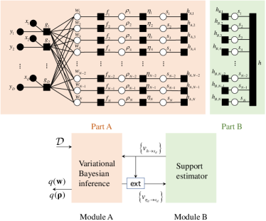
Figure 6: Illustration of the two modules in the Turbo-VBI algorithm.

Since the factor graph in Fig. 5 has loops, directly applying the message passing algorithm usually cannot achieve a good performance. In addition, since the probability model is more complicated than the existing ones in [15] and [16], it is difficult to directly apply the VBI algorithm. Thus, we consider separating the complicated probability model in Fig. 5 into two parts, and perform Bayesian inference respectively, as illustrated in Fig. 6. Specifically, we follow the turbo framework and divide the factor graph into two parts. One is the support part (Part B), which contains the prior information. The other one is the remaining part (Part A). Correspondingly, the proposed Turbo-VBI algorithm is also divided into two modules such that each module performs Bayesian inference on its corresponding part respectively. Module A and Module B also need to exchange messages. Specifically, the output message $v_{h\rightarrow s_{n}}$ of Module B refers to the message from factor node $h_{A,n}$ to variable node $s_{n}$ in Part A, and is equivalent to the message from variable node $s_{n}$ to factor node $h_{B,n}$ in Part B, which refers to the conditional marginal probability $p\left(s_{n}|\boldsymbol{v}_{\boldsymbol{\eta}\rightarrow\mathbf{s}}\right)$. It is calculated by sum-product message passing (SPMP) on part B, and acts as the input of Module A to facilitate the VBI on Part A. The output message $v_{\eta_{n}\rightarrow s_{n}}$ of Module A refers to the posterior probability subtracting the output of Module B: $\frac{q\left(s_{n}\right)}{v_{h\rightarrow s_{n}}}$, and acts as the input of Module B to facilitate SPMP on Part B.

Specifically, the probability model for the prior distribution in Part A is assumed as

$$\hat{p}\left(\mathbf{w},\boldsymbol{\rho},\mathbf{s}\right)=\hat{p}\left(\mathbf{s}\right)p\left(\boldsymbol{\rho}|\mathbf{s}\right)p\left(\mathbf{w}|\boldsymbol{\rho}\right),$$ (15)

where

$$\hat{p}\left(\mathbf{s}\right)=\prod_{n=1}^{N}\left(\pi_{n}\right)^{s_{n}}\left(1-\pi_{n}\right)^{1-s_{n}}$$

is a new prior for support $\mathbf{s}$. $\pi_{n}$ is the probability that $s_{n}=1$, which is defined as:

$$\pi_{n}=p\left(s_{n}=1\right)=\frac{v_{h\rightarrow s_{n}}\left(1\right)}{v_{h\rightarrow s_{n}}\left(1\right)+v_{h\rightarrow s_{n}}\left(0\right)}.$$ (16)

Note that the only difference between the new prior in (15) and that in (1) is that the complicated $p\left(\mathbf{s}\right)$ is replaced by a simpler distribution $\hat{p}\left(\mathbf{s}\right)$ with independent entries. The correlations among the supports are separated into Part B. Then, based on the new prior $\hat{p}\left(\mathbf{w},\boldsymbol{\rho},\mathbf{s}\right)$, Module A performs a VBI algorithm. In the VBI algorithm, variational distributions $q\left(\mathbf{w}\right)$, $q\left(\boldsymbol{\rho}\right)$ and $q\left(\mathbf{s}\right)$ are used to approximate the posterior. After that, the approximate posterior $q\left(\mathbf{s}\right)$ is delivered from Module A back into Module B. The delivered message $v_{\eta_{n}\rightarrow s_{n}}$ is defined as

$$v_{\eta_{n}\rightarrow s_{n}}=\frac{q\left(s_{n}\right)}{v_{h\rightarrow s_{n}}},$$ (17)

according to the sumproduct rule.

With the input message $v_{\eta_{n}\rightarrow s_{n}}$, Module B further performs SPMP over Part B to exploit the structured sparsity, which is contained in the prior distribution $p\left(\mathbf{s}\right).$ Specifically, in Part B, the factor nodes

$$h_{B,n}=v_{\eta_{n}\rightarrow s_{n}},n=1,...,N$$ (18)

carry the information of the variational posterior distribution $q\left(\mathbf{s}\right)$, and the factor node $h$ carries the structured prior information of $p\left(\mathbf{s}\right)$. By performing SPMP over Part B, the message $v_{h\rightarrow s_{n}}$ can be calculated and then delivered to Module A. These two modules exchange messages iteratively until convergence or the maximum iteration number is exceeded. After this, the final outputs $q\left(\mathbf{w}\right)$, $q\left(\boldsymbol{\rho}\right)$ and $q\left(\mathbf{s}\right)$ of Module A are the approximate posterior distribution for $\mathbf{w}$, $\boldsymbol{\rho},$ and $\mathbf{s}$, respectively. Note that although the SPMP is not guaranteed to converge on Part B, because our $p\left(\mathbf{s}\right)$ is an MRF prior, the desired structure is usually well promoted in the final output of Module A, as illustrated in the simulation results. This is because SPMP can achieve good results on 2-D Ising model and there have been many solid works concerning SPMP on loopy graphs [27]. And our proposed VBI compression algorithm in Module A can achieve good enough performance to capture the structure. In addition, since the design of $p\left(\mathbf{s}\right)$ is flexible, one can model it with Markov chain priors or Markov tree priors. In this case, the convergence is guaranteed. In the following, we elaborate the two modules in details.

IV-B Sparse VBI Estimator (Module A)

In Module A, we want to use a tractable variational distribution $q\left(\mathbf{w},\boldsymbol{\rho},\mathbf{s}\right)$ to approximate the intractable posterior distribution $\hat{p}\left(\mathbf{w},\boldsymbol{\rho},\mathbf{s}|\mathcal{D}\right)$ under the prior $\hat{p}\left(\mathbf{w},\boldsymbol{\rho},\mathbf{s}\right)$. The quality of this approximation is measured by the Kullback-Leibler divergence (KL divergence):

$$D_{KL}\left(q\left(\mathbf{w},\boldsymbol{\rho},\mathbf{s}\right)||\hat{p}\left(\mathbf{w},\boldsymbol{\rho},\mathbf{s}|\mathcal{D}\right)\right)\\ =\sum_{\mathbf{s}}\int\int q\left(\mathbf{w},\boldsymbol{\rho},\mathbf{s}\right)\ln\frac{q\left(\mathbf{w},\boldsymbol{\rho},\mathbf{s}\right)}{\hat{p}\left(\mathbf{w},\boldsymbol{\rho},\mathbf{s}|\mathcal{D}\right)}d\mathbf{w}d\boldsymbol{\rho}.$$ (19)

Thus, the goal is to find the optimal variational distribution $q\left(\mathbf{w},\boldsymbol{\rho},\mathbf{s}\right)$ that minimizes this KL divergence. However, the KL divergence still involves calculating the intractable posterior $\hat{p}\left(\mathbf{w},\boldsymbol{\rho},\mathbf{s}|\mathcal{D}\right)$. In order to overcome this challenge, the minimization of KL divergence is usually transformed into a minimization of the negative evidence lower bound (ELBO), subject to a factorized form constraint [28].

Sparse VBI Problem:

$$\min_{q\left(\mathbf{w},\boldsymbol{\rho},\mathbf{s}\right)} -ELBO,$$ (20)

$$s.t. q\left(\mathbf{w},\boldsymbol{\rho},\mathbf{s}\right)=\prod_{n=1}^{N}q\left(w_{n}\right)q\left(\rho_{n}\right)q\left(s_{n}\right),$$

where $ELBO=\sum_{\mathbf{s}}\int\int q\left(\mathbf{w},\boldsymbol{\rho},\mathbf{s}\right)\ln p\left(\mathcal{D}|\mathbf{w},\boldsymbol{\rho},\mathbf{s}\right)d\mathbf{w}d\boldsymbol{\rho}-D_{KL}\left(q\left(\mathbf{w},\boldsymbol{\rho},\mathbf{s}\right)||\hat{p}\left(\mathbf{w},\boldsymbol{\rho},\mathbf{s}\right)\right).$ The constraint means all individual variables $w,\rho$ and $s$ are assumed to be independent. Such an assumption is known as the mean field assumption and is widely used in VBI methods [16, 28].

The problem in (20) is non-convex and generally we can only achieve a stationary solution $q^{*}\left(\mathbf{w},\boldsymbol{\rho},\mathbf{s}\right)$. A stationary solution can be achieved by applying a block coordinate descent (BCD) algorithm to the problem in (20), as will be proved in Lemma 1. According to the idea of the BCD algorithm, to solve (20) is equivalent to iteratively solving the following three subproblems.

Subproblem 1 (update of $\boldsymbol{\rho}$):

$$\min_{q\left(\boldsymbol{\rho}\right)} D_{KL}\left(q\left(\boldsymbol{\rho}\right)||\widetilde{p}_{\boldsymbol{\rho}}\right),$$ (21)

$$s.t. q\left(\boldsymbol{\rho}\right)=\prod_{n=1}^{N}q\left(\rho_{n}\right),$$

where $\ln\widetilde{p}_{\boldsymbol{\rho}}=\left\langle\ln\hat{p}\left(\mathbf{w},\boldsymbol{\rho},\mathbf{s},\mathcal{D}\right)\right\rangle_{q\left(\mathbf{s}\right)q\left(\mathbf{w}\right)}.$

Subproblem 2 (update of $\mathbf{s}$):

$$\min_{q\left(\mathbf{s}\right)} D_{KL}\left(q\left(\boldsymbol{s}\right)||\widetilde{p}_{\mathbf{s}}\right),$$ (22)

$$s.t. q\left(\mathbf{s}\right)=\prod_{n=1}^{N}q\left(s_{n}\right),$$

where $\ln\widetilde{p}_{\mathbf{s}}=\left\langle\ln\hat{p}\left(\mathbf{w},\boldsymbol{\rho},\mathbf{s},\mathcal{D}\right)\right\rangle_{q\left(\boldsymbol{\rho}\right)q\left(\mathbf{w}\right)}.$

Subproblem 3 (update of $\mathbf{w}$):

$$\min_{q\left(\mathbf{w}\right)} D_{KL}\left(q\left(\mathbf{w}\right)||\widetilde{p}_{\mathbf{w}}\right),$$ (23)

$$s.t. q\left(\mathbf{w}\right)=\prod_{n=1}^{N}q\left(w_{n}\right),$$

where $\ln\widetilde{p}_{\mathbf{w}}=\left\langle\ln\hat{p}\left(\mathbf{w},\boldsymbol{\rho},\mathbf{s},\mathcal{D}\right)\right\rangle_{q\left(\boldsymbol{\rho}\right)q\left(\mathbf{s}\right)}$ and $\left\langle f\left(x\right)\right\rangle_{q\left(x\right)}=\int f\left(x\right)q\left(x\right)dx.$ The detailed derivations of the three subproblems are provided in the Appendix A. In the following, we elaborate on solving the three subproblems respectively.

1) Update of $q\left(\boldsymbol{\rho}\right)$: In subproblem 1, obviously, the optimal solution $q^{\star}\left(\boldsymbol{\rho}\right)$ is achieved when $q^{\star}\left(\boldsymbol{\rho}\right)=\widetilde{p}_{\boldsymbol{\rho}}$. In this case, $q^{\star}\left(\boldsymbol{\rho}\right)$ can be derived as

$$q^{\star}\left(\boldsymbol{\rho}\right)=\prod_{n=1}^{N}\Gamma\left(\rho_{n};\widetilde{a}_{n},\widetilde{b}_{n}\right),$$ (24)

where $\widetilde{a}_{n}$ and $\widetilde{b}_{n}$ are given by:

$$\widetilde{a}_{n} =\left\langle s_{n}\right\rangle a_{n}+\left\langle 1-s_{n}\right\rangle\overline{a}_{n}+1$$ (25)

$$=\widetilde{\pi}_{n}a_{n}+\left(1-\widetilde{\pi}_{n}\right)\overline{a}_{n}+1,$$

$$\widetilde{b}_{n} =\left\langle|w_{n}|^{2}\right\rangle+\left\langle s_{n}\right\rangle b_{n}+\left\langle 1-s_{n}\right\rangle\overline{b}_{n}$$ (26)

$$=|\mu_{n}|^{2}+\sigma_{n}^{2}+\widetilde{\pi}_{n}b_{n}+\left(1-\widetilde{\pi}_{n}\right)\overline{b}_{n},$$

where $\mu_{n}$ and $\sigma_{n}^{2}$ are the posterior mean and variance of weight $w_{n}$ respectively, and $\widetilde{\pi}_{n}$ is the posterior expectation of $s_{n}$.

2) Update of $q\left(\mathbf{s}\right)$: In subproblem 2, we can achieve the optimal solution $q^{\star}\left(\mathbf{s}\right)$ by letting $q^{\star}\left(\mathbf{s}\right)=\widetilde{p}_{\mathbf{s}}$. In this case, $q^{\star}\left(\mathbf{s}\right)$ can be derived as

$$q^{\star}\left(\mathbf{s}\right)=\prod_{n=1}^{N}\left(\widetilde{\pi}_{n}\right)^{s_{n}}\left(1-\widetilde{\pi}_{n}\right)^{1-s_{n}},$$ (27)

where $\widetilde{\pi}_{n}=\frac{C_{1}}{C_{1}+C_{2}}.$ $C_{1}$ and $C_{2}$ are given by:

$$C_{1}=\frac{\pi_{n}b_{n}^{a_{n}}}{\Gamma\left(a_{n}\right)}e^{\left(a_{n}-1\right)\left\langle\ln\rho_{n}\right\rangle-b_{n}\left\langle\rho_{n}\right\rangle},$$ (28)

$$C_{2}=\frac{\left(1-\pi_{n}\right)\overline{b}_{n}^{\overline{a}_{n}}}{\Gamma\left(\overline{a}_{n}\right)}e^{\left(\overline{a}_{n}-1\right)\left\langle\ln\rho_{n}\right\rangle-\overline{b}_{n}\left\langle\rho_{n}\right\rangle},$$ (29)

where $\left\langle\ln\rho_{n}\right\rangle=\psi\left(\widetilde{a}_{n}\right)-\ln\left(\widetilde{b}_{n}\right)$, $\psi\left(x\right)=\frac{d}{dx}\ln\left(\Gamma\left(x\right)\right)$ is the digamma function. The detailed derivation of $q^{\star}\left(\boldsymbol{\rho}\right)$ and $q^{\star}\left(\mathbf{s}\right)$ is provided in the Appendix B.

3) Update of $q\left(\mathbf{w}\right)$: Expanding the objective function in subproblem 3, we have

$$D_{KL}\left(q\left(\mathbf{w}\right)||\widetilde{p}_{\mathbf{w}}\right)$$ (30)

$$=\mathbb{E}_{q\left(\mathbf{w}\right)}\ln q\left(\mathbf{w}\right)-\mathbb{E}_{q\left(\mathbf{w}\right)}\left[\left\langle\ln p\left(\mathbf{w},\boldsymbol{\rho},\mathbf{s},\mathcal{D}\right)\right\rangle_{q\left(\boldsymbol{\rho}\right)q\left(\mathbf{s}\right)}\right]$$

$$=\mathbb{E}_{q\left(\mathbf{w}\right)}\left(\ln q\left(\mathbf{w}\right)-\left\langle\ln p\left(\mathbf{w}|\boldsymbol{\rho}\right)\right\rangle_{q\left(\boldsymbol{\rho}\right)}\right)-\mathbb{E}_{q\left(\mathbf{w}\right)}\ln p\left(\mathcal{D}|\mathbf{w}\right)+const.$$

Similar to traditional variational Bayesian model compression [16, 15], the objective function (30) contains two parts: the “prior part” $\mathbb{E}_{q\left(\mathbf{w}\right)}\left(\ln q\left(\mathbf{w}\right)-\left\langle\ln p\left(\mathbf{w}|\boldsymbol{\rho}\right)\right\rangle_{q\left(\boldsymbol{\rho}\right)}\right)$ and the “data part” $\mathbb{E}_{q\left(\mathbf{w}\right)}\ln p\left(\mathcal{D}|\mathbf{w}\right)$. The prior part forces the weights to follow the prior distribution while the data part forces the weights to express the dataset. The only difference from traditional variational Bayesian model compression [16, 15] is that the prior term $\left\langle\ln p\left(\mathbf{w}|\boldsymbol{\rho}\right)\right\rangle_{q\left(\boldsymbol{\rho}\right)}$ is parameterized by $\boldsymbol{\rho}$ and $\boldsymbol{\rho}$ carries the structure captured by the three layer hierarchical prior. Our aim is to find the optimal $q\left(\mathbf{w}\right)$ that minimizes $D_{KL}\left(q\left(\mathbf{w}\right)||\widetilde{p}_{\mathbf{w}}\right)$, subject to the factorized constraint $q\left(\mathbf{w}\right)=\prod_{n=1}^{N}q\left(w_{n}\right)$. It can be observed that the objective function contains the likelihood term $\ln p\left(\mathcal{D}|\mathbf{w}\right)$, which can be very complicated for complex models. Thus, subproblem 3 is non-convex and it is difficult to obtain the optimal solution. In the following, we aim at finding a stationary solution $q^{*}\left(\mathbf{w}\right)$ for subproblem 3. There are several challenges in solving subproblem 3, summarized as follows.

Challenge 1: Closed form for the prior part $\mathbb{E}_{q\left(\mathbf{w}\right)}\left(\ln q\left(\mathbf{w}\right)-\left\langle\ln p\left(\mathbf{w}|\boldsymbol{\rho}\right)\right\rangle_{q\left(\boldsymbol{\rho}\right)}\right)$. In traditional variational Bayesian model compression, this expectation is usually calculated by approximation [15], which involves approximating error. To calculate the expectation accurately, a closed form for this expectation is required. Challenge 2: Low-complexity deterministic approximation for the data part $\mathbb{E}_{q\left(\mathbf{w}\right)}\ln p\left(\mathcal{D}|\mathbf{w}\right)$. In traditional variational Bayesian model compression [16, 15], this intractable expectation is usually approximated by Monte Carlo sampling. However, Monte Carlo approximation has been pointed out to have high complexity and low robustness. In addition, the variance of the Monte Carlo gradient estimates is difficult to control [19]. Thus, a low-complexity deterministic approximation for the likelihood term is required.

Closed form for $\mathbb{E}_{q\left(\mathbf{w}\right)}\left(\ln q\left(\mathbf{w}\right)-\left\langle\ln p\left(\mathbf{w}|\boldsymbol{\rho}\right)\right\rangle_{q\left(\boldsymbol{\rho}\right)}\right)$. To overcome Challenge 1, we propose to use a Gaussian distribution as the approximate posterior. That is, $q\left(w_{n}\right)=\mathcal{N}\left(\mu_{n},\sigma_{n}^{2}\right)$, $q\left(\mathbf{w}\right)=\prod_{n=1}^{N}q\left(w_{n}\right)$, $\mu_{n}$ and $\sigma_{n}^{2}$ are the variational parameters that we want to optimize. Then, since the prior $p\left(\mathbf{w}|\boldsymbol{\rho}\right)$ is also chosen as a Gaussian distribution, $\mathbb{E}_{q\left(\mathbf{w}\right)}\left(\ln q\left(\mathbf{w}\right)-\left\langle\ln p\left(\mathbf{w}|\boldsymbol{\rho}\right)\right\rangle_{q\left(\boldsymbol{\rho}\right)}\right)$ can be written as the KL-divergence between two Gaussian distributions. Thus, the expectation has a closed form and can be calculated up to a constant. Specifically, by expanding $p\left(\mathbf{w}|\boldsymbol{\rho}\right)$, we have

$$\left\langle\ln p\left(\mathbf{w}|\boldsymbol{\rho}\right)\right\rangle =\sum_{n=1}^{N}\left\langle\ln\sqrt{\frac{\rho_{n}}{2\pi}}e^{-\frac{w_{n}^{2}}{2}\rho_{n}}\right\rangle$$ (31)

$$=\sum_{n=1}^{N}\left\langle\frac{1}{2}\ln\rho_{n}-\frac{w_{n}^{2}}{2}\rho_{n}+const.\right\rangle$$

$$=\sum_{n=1}^{N}\left(\frac{1}{2}\left\langle\ln\rho_{n}\right\rangle-\frac{w_{n}^{2}}{2}\left\langle\rho_{n}\right\rangle+const.\right)$$

$$=\sum_{n=1}^{N}\left(\ln p\left(w_{n}|\left\langle\rho_{n}\right\rangle\right)+const.\right)$$

$$=\ln p\left(\mathbf{w}|\left\langle\boldsymbol{\rho}\right\rangle\right)+const.,$$

where we use $\left\langle\cdot\right\rangle$ to replace $\left\langle\cdot\right\rangle_{q\left(\boldsymbol{\rho}\right)}$ or $\left\langle\cdot\right\rangle_{q\left(\rho\right)}$ for simplicity. Thus, we have

$$\mathbb{E}_{q\left(\mathbf{w}\right)}\left(\ln q\left(\mathbf{w}\right)-\left\langle\ln p\left(\mathbf{w}|\boldsymbol{\rho}\right)\right\rangle_{q\left(\boldsymbol{\rho}\right)}\right)\\ =\mathbb{E}_{q\left(\mathbf{w}\right)}\left(\ln q\left(\mathbf{w}\right)-\ln p\left(\mathbf{w}|\mathbb{E}\left[\boldsymbol{\rho}\right]\right)\right)+const.\\ =D_{KL}\left(q\left(\mathbf{w}\right)||p\left(\mathbf{w}|\mathbb{E}\left[\boldsymbol{\rho}\right]\right)\right)+const..$$ (32)

Since $q\left(\mathbf{w}\right)$ and $p\left(\mathbf{w}|\mathbb{E}\left[\boldsymbol{\rho}\right]\right)$ are both Gaussian distributions, the KL-divergence between them has a closed form:

$$D_{KL}\left(q\left(\mathbf{w}\right)||p\left(\mathbf{w}|\mathbb{E}\left[\boldsymbol{\rho}\right]\right)\right)=\sum_{n=1}^{N}\left(\ln\frac{\widetilde{\sigma}_{n}}{\sigma_{n}}+\frac{\sigma_{n}^{2}+\mu_{n}^{2}}{2\widetilde{\sigma}_{n}^{2}}-\frac{1}{2}\right),$$ (33)

where $\widetilde{\sigma}_{n}^{2}=\frac{1}{\mathbb{E}\left[\rho_{n}\right]}$ is the variance of the prior $p\left(\mathbf{w}|\mathbb{E}\left[\boldsymbol{\rho}\right]\right)$. Since our aim is to minimize (30), the constant term in (32) can be omitted.

Low-complexity deterministic approximation for $\mathbb{E}_{q\left(\mathbf{w}\right)}\ln p\left(\mathcal{D}|\mathbf{w}\right)$. To overcome Challenge 2, we propose a low-complexity deterministic approximation for $\mathbb{E}_{q\left(\mathbf{w}\right)}\ln p\left(\mathcal{D}|\mathbf{w}\right)$ based on Taylor expansion.

For simplicity, let $g\left(\mathbf{w}\right)$ denote the complicated function $\ln p\left(\mathcal{D}|\mathbf{w}\right)$. Specifically, we want to construct a deterministic approximation for $\mathbb{E}_{\mathbf{w}\sim q\left(\mathbf{w}\right)}g\left(\mathbf{w}\right)$ with the variational parameters $\mu_{n}$ and $\sigma_{n}^{2}$, $n=1,...,N$. Following the reparameterization trick in [15] and [29], we represent $w_{n}$ by $\mu_{n}+\xi_{n}\sigma_{n}^{2}$, $\xi_{n}\sim\mathcal{N}\left(0,1\right)$. In this way, $w_{n}$ is transformed into a deterministic differentiable function of a non-parametric noise $\xi_{n}$, and $\mathbb{E}_{\mathbf{w}\sim q\left(\mathbf{w}\right)}g\left(\mathbf{w}\right)$ is transformed into $\mathbb{E}_{\boldsymbol{\xi}\sim\mathcal{N}\left(0,1\right)}g\left(\boldsymbol{\mu}+\boldsymbol{\xi\sigma^{2}}\right)$. Note that in traditional variational Bayesian model compression, this expectation is approximated by sampling $\boldsymbol{\xi}$. However, to construct a deterministic approximation, we take the first-order Taylor approximation of $\mathbb{E}_{\boldsymbol{\xi}\sim\mathcal{N}\left(0,1\right)}g\left(\boldsymbol{\mu}+\boldsymbol{\xi\sigma^{2}}\right)$ at the point $\boldsymbol{\xi}=\mathbb{E}\left[\boldsymbol{\xi}\right]=\mathbf{0}$, and we have

$$\mathbb{E}_{\boldsymbol{\xi}}g\left(\boldsymbol{\mu}+\boldsymbol{\xi\sigma^{2}}\right)\approx g\left(\boldsymbol{\mu}+\mathbb{E}\left[\boldsymbol{\xi}\right]\cdot\boldsymbol{\sigma^{2}}\right)=g\left(\boldsymbol{\mu}\right).$$ (34)

That is, we use the first-order Taylor approximation to replace $\mathbb{E}_{\boldsymbol{\xi}}g\left(\boldsymbol{\mu}+\boldsymbol{\xi\sigma^{2}}\right)$. Simulation results show that our proposed approximation can achieve good performance. Additionally, since our proposed approximation is deterministic, the gradient variance can be eliminated.

Based on the aforementioned discussion , subproblem 3 can be solved by solving an approximated problem as follows.

Approx. Subproblem 3:

$$\min_{\boldsymbol{\mu},\boldsymbol{\sigma}^{2}} \sum_{n=1}^{N}\left(\ln\frac{\widetilde{\sigma}_{n}}{\sigma_{n}}+\frac{\sigma_{n}^{2}+\mu_{n}^{2}}{2\widetilde{\sigma}_{n}^{2}}-\frac{1}{2}\right)-\ln p\left(\mathcal{D}|\boldsymbol{\mu}\right).$$ (35)

This problem is equivalent to training a Bayesian neural network with (35) as the loss function.

4) Convergence of Sparse VBI: The sparse VBI in Module A is actually a BCD algorithm to solve the problem in (20). By the physical meaning of ELBO and KL divergence, the objective function is continuous on a compact level set. In addition, the objective function has a unique minimum for two coordinate blocks ($q\left(\boldsymbol{\rho}\right)$ and $q\left(\mathbf{s}\right)$) [17, 28]. Since we can achieve a stationary point for the third coordinate block $q\left(\mathbf{w}\right)$, the objective function is regular at the cluster points generated by the BCD algorithm. Based on the above discussion, our proposed BCD algorithm satisfies the BCD algorithm convergence requirements in [30]. Thus, we have the following convergence lemma.

Lemma 1.

(Convergence of Sparse VBI): Every cluster point $q^{*}\left(\mathbf{w},\boldsymbol{\rho},\mathbf{s}\right)=q^{\star}\left(\boldsymbol{\rho}\right)q^{\star}\left(\mathbf{s}\right)q^{*}\left(\mathbf{w}\right)$ generated by the sparse VBI algorithm is a stationary solution of problem (20).

IV-C Message Passing (Module B)

In Module B, SPMP is performed on the support factor graph $\mathcal{G}_{s}$ and the normalized message $v_{s_{n}\rightarrow h_{B}}$ is fed back to Module A as the prior probability $\hat{p}\left(s_{n}\right)$.

Figure 7: Illustration of the support factor graph in Module B with $K$ input neurons and $M$ output neurons.

1:training set $\mathcal{D}$, priors $p\left(\mathbf{w}\right)$, $p\left(\boldsymbol{\rho}\right)$, $p\left(\mathbf{s}\right)$, maximum iteration number $I_{max}$.

2:$\mathbf{w}^{*}$, $\boldsymbol{\rho}^{*}$, $\mathbf{s}^{*}$.

3:Initialize $\pi_{n}$.

4:for $k=1,...,I_{m}$ do

5:     Module A:

6:     Initialize the variational distribution $q\left(\boldsymbol{\rho}\right)$ and $q\left(\mathbf{s}\right)$.

7:     while not converged do

8:         Update $q\left(\boldsymbol{\rho}\right)$, $q\left(\mathbf{s}\right)$ and $q\left(\mathbf{w}\right)$.

9:     end while

10:     Calculate $v_{\eta_{n}\rightarrow s_{n}}$ based on $(17)$ and send $v_{\eta_{n}\rightarrow s_{n}}$ to Module B.

11:     Module B:

12:     Perform SPMP on $\mathcal{G}_{s}$, send $v_{h\rightarrow s_{n}}$ to Module A.

13:     if converge then

14:         break

15:     end if

16:     $k=k+1$.

17:end for

18:Output $\mathbf{w}^{*}=\arg\max_{\mathbf{w}}q^{*}\left(\mathbf{w}\right)$, $\boldsymbol{\rho}^{*}=\arg\max_{\boldsymbol{\rho}}q^{\star}\left(\boldsymbol{\rho}\right)$, $\mathbf{s}^{*}=\arg\max_{\mathbf{s}}q^{\star}\left(\mathbf{s}\right)$.

Algorithm 1 Turbo-VBI Algorithm for Model Compression

We focus on one fully connected layer with $K$ input neurons and $M$ output neurons for easy elaboration. The support prior $p\left(\mathbf{s}\right)$ for this $K\times M$ layer is modeled as an MRF. The factor graph $\mathcal{G}_{s}$ is illustrated in Fig. 7. Here we use $s_{i,j}$ to denote the support variable in the $i$-th row and $j$-th column. The unary factor node $h_{B,i,j}$ carries the probability given by (18). The pair-wise factor nodes carry the row and column transition probability $p\left(s_{row,m+1}|s_{row,m}\right)$ and $p\left(s_{col,k+1}|s_{col,k}\right)$, respectively. The parameters $p_{01}^{row},p_{10}^{row}$ and $p_{01}^{col},p_{10}^{col}$ for the MRF model are given in Section II-C. Let $v_{s\rightarrow f}\left(s\right)$ denote the message from the variable node $s$ to the factor node $f$, and $v_{f\rightarrow s}\left(s\right)$ denote the message from the factor node $f$ to the variable node $s$. According to the sum-product law, the messages are updated as follows:

$$v_{s\rightarrow f}\left(s\right)=\prod_{h\in n\left(s\right)\setminus\{f\}}v_{h\rightarrow s}\left(s\right),$$ (36)

$$v_{f\rightarrow s}\left(s\right)=\begin{cases}f\left(s\right)&f\;is\;unary\;factor\;node,\\ f\left(s\right)\cdot v_{t\rightarrow f}\left(t\right)&f\;is\;pairwise\;factor\;node,\end{cases}$$ (37)

where $n\left(s\right)\setminus\{f\}$ denotes the neighbour factor nodes of $s$ except node $f$, and $t$ denotes the other neighbour variable node of $f$ except node $s$. After the SPMP algorithm is performed, the final message $v_{s\rightarrow h_{B}}$ from each variable node $s_{i,j}$ to the connected unary factor node $h_{B,i,j}$ is sent back to Module A.

The overall algorithm is summarized in Algorithm 1.

Remark 2. (Comparison with traditional variational inference) Traditional variational inference cannot handle the proposed three-layer sparse prior $p\left(\mathbf{w},\boldsymbol{\rho},\mathbf{s}\right)$ while our proposed Turbo-VBI is specially designed to handle it. In existing Bayesian compression works [14]-[16], the KL-divergence between the true posterior $p\left(\mathbf{w}|\mathcal{D}\right)$ and the variational posterior $q\left(\mathbf{w}\right)$ is easy to calculate, so that the KL-divergence can be directly optimized. Thus, simple variational inference can be directly applied. The fundamental reason behind this is that the prior $p\left(\mathbf{w}\right)$ in these works are relatively simple, and they usually only have one layer [14, 15] or two layers [16]. Thus, the KL-divergence between the prior $p\left(\mathbf{w}\right)$ and the variational posterior $q\left(\mathbf{w}\right)$ is easy to calculate, which is a must in calculating the KL-divergence between the true posterior $p\left(\mathbf{w}|\mathcal{D}\right)$ and the variational posterior $q\left(\mathbf{w}\right)$. However, these simple priors cannot promote the desired regular structure in the weight matrix and lack the flexibility to configure the pruned structure. Thus, we introduce the extra support layer $\mathbf{s}$, which leads to the three layer hierarchical prior $p\left(\mathbf{w},\boldsymbol{\rho},\mathbf{s}\right)$. With this three-layer prior, traditional variational inference cannot be applied because the KL-divergence between the prior $p\left(\mathbf{w},\boldsymbol{\rho},\mathbf{s}\right)$ and the variational posterior $q\left(\mathbf{w},\boldsymbol{\rho},\mathbf{s}\right)$ is difficult to calculate. In order to inference the posterior, we propose to separate the factor graph into two parts and iteratively perform Bayesian inference, which leads to our proposed Turbo-VBI algorithm.

V Performance Analysis

In this section, we evaluate the performance of our proposed Turbo-VBI based model compression method on some standard neural network models and datasets. We also compare with several baselines, including classic and state-of-the-art model compression methods. The baselines considered are listed as follows:

1. Variational dropout (VD): This is a very classic method in the area of Bayesian model compression, which is proposed in [15]. A single-layer improper log-uniform prior is assigned to each weight to induce sparsity during training.

2. Group variational dropout (GVD): This is proposed in [16], which can be regarded as an extension of VD into group pruning. In this algorithm, each weight follows a zero-mean Gaussian prior. The prior scales of the weights in the same group jointly follow an improper log-uniform distribution or a proper half-Cauchy distribution to realize group pruning. In this paper, we choose the improper log-uniform prior for comparison. Note that some more recent Bayesian compression methods mainly focus on a quantization perspective [14, 31], which is a different scope from our work. Although our work can be further extended into quantization area, we only focus on structured pruning here. To our best knowledge, GVD is still one of the state-of-the-art Bayesian pruning methods without considering quantization.

3. Polarization regularizer based pruning (polarization): This is proposed in [9]. The algorithm can push some groups of weights to zero while others to larger values by assigning a polarization regularizer to the batch norm scaling factor of each weight group

   $$\min_{\mathbf{w}} \frac{1}{D}\sum_{d=1}^{D}L\left(NN\left(x_{d},\mathbf{w}\right),y_{d}\right)+R\left(\mathbf{w}\right)$$

   $$+\lambda\left(t\left\|\boldsymbol{\gamma}\right\|_{1}-\left\|\boldsymbol{\gamma}-\bar{\gamma}\mathbf{1}_{n}\right\|_{1}\right),$$

   where $\lambda\left(t\left\|\boldsymbol{\gamma}\right\|_{1}-\left\|\boldsymbol{\gamma}-\bar{\gamma}\mathbf{1}_{n}\right\|_{1}\right)$ is the proposed polarization regularizer and $\boldsymbol{\gamma}$ is the batch norm scaling factor of each weight.

4. Single-shot network pruning (SNIP): This is proposed in [1]. The algorithm measures the weight importance by introducing an auxiliary variable to each weight. The importance of each weight is achieved before training by calculating the gradient of its “importance variable”. After this, the weights with less importance are pruned before the normal training.

We perform experiments on LeNet-5, AlexNet, and VGG-11 architectures, and use the following benchmark datasets for the performance comparison.

1. Fashion-MNIST [32]: It consists of a training set of 60000 examples and a test set of 10000 examples. Each example is a $28\times 28$ grayscale image of real life fashion apparel, associated with a label from 10 classes.

2. CIFAR-10 [33]: It is the most widely used dataset to compare neural network pruning methods. It consists of a training set of 50000 examples and a test set of 10000 examples. Each example is a three-channel $32\times 32$ RGB image of real life object, associated with a label from 10 classes.

3. CIFAR-100 [33]: It is considered as a harder version of CIFAR-10 dataset. Instead of 10 classes in CIFAR-10, it consists of 100 classes with each class containing 600 images. There are 500 training images and 100 testing images in each class.

We will compare our proposed Turbo-VBI based model compression method with the baselines from different dimensions, including 1) an overall performance comparison; 2) visualization of the weight matrix structure; 3) CPU and GPU acceleration and 4) robustness of the pruned neural network.

We run LeNet-5 on Fashion-MNIST, and AlexNet on CIFAR-10 and VGG on CIFAR-100. Throughout the experiments, we set the learning rate as 0.01, and $a=b=\overline{a}=1,\overline{b}=1\times 10^{-3}$. For LeNet-5+Fashion-MNIST, we set the batch size as 64, and for AlexNet+CIFAR-10 and VGG+CIFAR-100, we set the batchsize as 128 . All the methods except for SNIP go through a fine tuning after pruning. For LeNet, the fine tuning is 15 epochs while for AlexNet and VGG, the fine tuning is 30 epochs. Note that the models and parameter settings may not achieve state-of-the-art accuracy but it is enough for comparison.

V-A Overall Performance Comparison

Network	Method	Accuracy (%)	$\frac{|\mathbf{w}\neq 0|}{|\mathbf{w}|}$ (%)	Pruned structure	FLOPs reduction (%)
	No pruning	89.01	100	6-16-120-84	0
	VD	88.91	6.16	6-15-49-51	11.82
LeNet-5	GVD	88.13	4.20	5-7-21-23	53.89
6-16-120-84	Polarization	87.27	17.96	4-8-46-27	59.04
	SNIP	82.83	9.68	5-16-73-57	19.82
	Proposed	88.77	1.14	3-5-16-17	76.03

(a) Results on LeNet+Fashion-MNIST.

Network	Method	Accuracy (%)	$\frac{|\mathbf{w}\neq 0|}{|\mathbf{w}|}$ (%)	Pruned structure	FLOPs reduction (%)
	No pruning	66.18	100	6-16-32-64-128-120-84	0
	VD	64.91	3.17	6-16-31-61-117-42-74	6.12
AlexNet	GVD	64.82	9.30	6-16-27-31-21-17-14	39.29
6-16-32-64-128-120-84	Polarization	63.95	25.95	4-15-16-20-19-58-53	65.27
	SNIP	63.19	11.75	6-16-30-57-102-56-68	12.51
	Proposed	65.57	3.42	6-16-25-20-7-7-7	45.94

(b) Results on AlexNet+CIFAR-10.

Network	Method	Accuracy (%)	$\frac{|\mathbf{w}\neq 0|}{|\mathbf{w}|}$ (%)	Pruned structure	FLOPs reduction (%)
	No pruning	68.28	100	64-128-256-256-512-512-512-512-100	0
	VD	67.24	5.39	64-128-256-211-447-411-293-279-44	16.63
VGG-11	GVD	66.52	9.05	63-112-204-134-271-174-91-77-33	60.90
64-128-256-256-512-512-512-512-100	Polarization	64.41	26.74	62-122-195-148- 291-133-76-74-68	59.54
	SNIP	65.20	17.79	64-128-254-246-441-479-371-274-69	7.92
	Proposed	67.12	4.68	60-119-191-148- 181-176-44-64-59	63.14

(c) Results on VGG11+CIFAR-100.

TABLE II: Overall performance comparisons to the baselines on different network models and datasets. Top-1 accuracy is reported. The best results are bolded.

We first give an overall performance comparison of different methods in terms of accuracy, sparsity rate, pruned structure and FLOPs reduction. The results are summarized in Table II. The structure is measured by output channels for convolutional layers and neurons for fully connected layers. It can be observed that our proposed method can achieve an extremely low sparsity rate, which is at the same level (or even lower than) the unstructured pruning methods (VD and SNIP). Moreover, it can also achieve an even more compact pruned structure than the structured pruning methods (polarization and GVD). At the same time, our proposed method can maintain a competitive accuracy. We summarize that the superior performance of our proposed method comes from two aspects: 1) superior individual weight pruning ability, which leads to low sparsity rate, and 2) superior neuron pruning ability, which leads to low FLOPs. Compared to random pruning methods like VD and SNIP which generally can achieve lower sparsity rate than group pruning methods, our proposed method can achieve even lower sparsity rate. This shows that our proposed sparse prior has high efficiency in pruning individual weights. This is because the regularization ability of $p\left(\mathbf{w|\boldsymbol{\rho}}\right)$ can be configured by setting small $\overline{b}$. Compared to group pruning methods like GVD and polarization, our proposed method can achieve a more compact structure. This shows our proposed method is also highly efficient in pruning neurons. The reason is two fold: First, each row in the prior $p\left(\mathbf{s}\right)$ can be viewed as a Markov chain. When some weights of a neuron are pruned, the other weights will also have a very high probability to be pruned. Second, the surviving weights in a weight matrix tend to gather in clusters, which means the surviving weights of different neurons in one layer tend to activate the same neurons in the next layer. This greatly improves the regularity from the input side, while the existing group pruning methods like GVD and polarization can only regularize the output side of a neuron.Visualization of Pruned Structure

Figure 8: Kernel structures of CONV_1 in LeNet.

In this subsection, we visualize the pruned weight matrix of our proposed method and compare to the baselines to further elaborate the benefits brought by the proposed regular structure. Fig. 8 illustrates the 6 kernels in the first layer of LeNet. We choose GVD and polarization for comparison here because these two are also structured pruning methods. It can be observed that GVD and polarization can both prune the entire kernels but the weights in the remaining kernels cannot be pruned and have no structure at all. However, in our proposed method, the weights in the remaining kernels are clearly pruned in a structured manner. In particular, we find that the three remaining $5\times 5$ kernels all fit in smaller kernels with size $3\times 3$. This clearly illustrates the clustered structure promoted by the MRF prior. With the clustered pruning, we can directly replace the original large kernels with smaller kernels, and enjoy the storage and computation benefits of the smaller kernel size.

V-B Acceleration Performance

(a) Avg. inferencing time on CPU.

(b) Avg. inferencing time on GPU.

Figure 9: Avg. time costed by one forward pass of a batch on CPU and GPU. For LeNet and AlexNet, the batch size is 10000 examples and each results is averaged on 1000 experiments. For VGG, the batch size is 1000 examples and each result is averaged on 100 experiments.

In this subsection, we compare the acceleration performance of our proposed method to the baselines. Note that the primary goal of the structured pruning is to reduce the computational complexity and accelerate the inference of the neural networks. In the weight matrix of our proposed method, we record the clusters larger than $3\times 3$ as an entirety. That is, we record the location and size of the clusters instead of recording the exact location for each element. In Fig. 9, we plot the average time costed by one forward pass of a batch on CPU and GPU respectively. It can be observed that our proposed method can achieve the best acceleration performance on different models. For LeNet, our proposed method can achieve a $1.50\times$ gain on CPU and $2.85\times$ gain on GPU. For AlexNet, the results are $1.63\times$ and $1.64\times$. For VGG, the results are $2.19\times$ and $1.88\times$. Note that the unstructured pruning methods show little acceleration gain because their sparse structure is totally random. We summarize the reason for our acceleration gain from two aspects: 1) More efficient neuron pruning. As shown in subsection V-A, our proposed method can result in a more compact model and thus leading to a larger FLOPs reduction. 2) More efficient decoding of weight matrix. Existing methods require to store the exact location for each unpruned weight, no matter in CSR, CSC or COO format because the sparse structure is irregular. However, in our proposed method, we only need the location and size for each cluster to decode all the unpruned weights in the cluster. Thus, the decoding is much faster. Note that the performance of our proposed method can be further improved if the structure is explored during the matrix-matrix multiplication. For example, the zero blocks can be skipped in matrix tiling, as discussed in subsection V-A. However, this involves modification in lower-level CUDA codes so we do not study it here.

V-C Insight Into the Proposed Algorithm

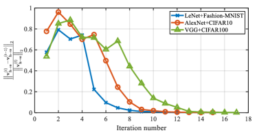
Figure 10: Convergence of proposed algorithm. The convergence if measured by the change in message $\boldsymbol{v}_{h\rightarrow s_{n}}$.

Figure 11: Visualization of the message $\boldsymbol{v}_{h\rightarrow s_{n}}$ and $\boldsymbol{v}_{\eta_{n}\rightarrow s_{n}}$ for the Dense_3 layer of AlexNet. $\boldsymbol{v}_{h\rightarrow s_{n}}$ carries the prior information of support from Module B and $\boldsymbol{v}_{\eta_{n}\rightarrow s_{n}}$ carries the posterior information of support from Module A. It can be clearly observed that the structured prior captured from Module B gradually regularizes the posterior. Eventually both $\boldsymbol{v}_{h\rightarrow s_{n}}$ and $\boldsymbol{v}_{\eta_{n}\rightarrow s_{n}}$ converge to a stable state.

In this subection, we provide some insight into the proposed method. First, Fig. 10 illustrates the convergence behavior of our proposed method on different tasks. It can be observed that generally our proposed method can converge in 15 iterations in all the tasks. Second, we illustrate how the structure is gradually captured by the prior information $\boldsymbol{v}_{h\rightarrow s_{n}}$ from Module B and how the posterior in Module A is regularized to this structure. As the clustered structure in kernels has been illustrated in Fig. 8, here in Fig. 11, we visualize the message $\boldsymbol{v}_{h\rightarrow s_{n}}$ and $\boldsymbol{v}_{\eta_{n}\rightarrow s_{n}}$ of the FC_3 layer in AlexNet. It can be observed that in iteration 1, the message $\boldsymbol{v}_{\eta_{n}\rightarrow s_{n}}$ has no structure because the prior $\hat{p}\left(\mathbf{s}\right)$ in Module A is randomly initialized. During the iterations of the algorithm, $\boldsymbol{v}_{\eta_{n}\rightarrow s_{n}}$ from Module B gradually captures the structure from the MRF prior and acts as a regularization in Module A, so that structure is gradually promoted in $\boldsymbol{v}_{h\rightarrow s_{n}}$. Finally, the support matrix has a clustered structure and the weight matrix also has a similar structure.

V-D Robustness of Pruned Model

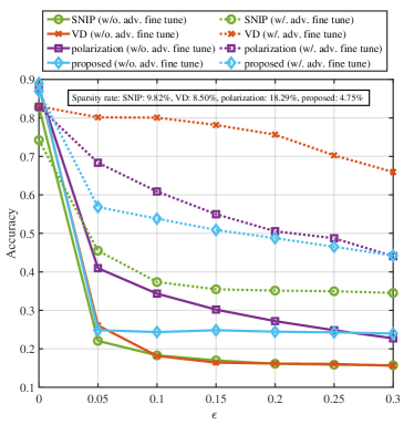
Figure 12: Accuracy vs $\epsilon$ for LeNet model.

In this subsection, we evaluate the robustness of the pruned model. The robustness of the pruned model is often neglected in model pruning methods while it is of highly importance [34, 35, 36]. We compare the model robustness of our proposed method to the baselines on LeNet and Fashion-MNIST dataset. We generate 10000 adversarial examples by fast gradient sign method (FGSM) and pass them through the pruned models. In Fig. 12, we plot the model accuracy under different $\epsilon$. Both the accuracy with and without an adversarial fine tuning is reported. It can be observed that all methods show a rapid drop without fine tuning. Specifically, our proposed method shows an accuracy drop of 72.1% from 89.01% when $\epsilon=0$ to 24.86% when $\epsilon=0.05$, while SNIP reports the largest drop of 73.4%. However, we also observe that the structured pruning methods (proposed and polarization) show stronger robustness than the unstructured ones (VD and SNIP). We think the reasons why our proposed method and polarization perform better may be different. For polarization, the unpruned weights are significantly more than other baselines, which means the remaining important filters have significantly more parameters. This allows the model to have a strong ability to resist the noise. For our proposed method, the possible reason is that it can enforce the weights to gather in groups. Thus, the model can “concentrate” on some specific features even when they are added by noise. It can be observed that after an adversarial fine tuning, all methods show an improvement. VD shows the largest improvement of 77.31% at $\epsilon=0.1$ while our proposed method only shows a moderate improvement of 56.26%. The possible reason behind this is our proposed method is “too” sparse and the remaining weights cannot learn the new features. Note that SNIP shows the smallest improvement. The possible reason is that in SNIP, the weights are pruned before training and the auxiliary importance variables may not measure the weight importance accurately, which results in some important weights being pruned. Thus, the expressing ability of the model may be harmed.

VI Conclusions and Future Work

Conclusions

We considered the problem of model compression from a Bayesian perspective. We first proposed a three-layer hierarchical sparse prior in which an extra support layer is used to capture the desired structure for the weights. Thus, the proposed sparse prior can promote both per-neuron weight-level structured sparsity and neuron-level structured sparsity. Then, we derived a Turbo-VBI based Bayesian compression algorithm for the resulting model compression problem. Our proposed algorithm has low complexity and high robustness. We further established the convergence of the sparse VBI part in the Turbo-VBI algorithm. Simulation results show that our proposed Turbo-VBI based model compression algorithm can promote a more regular structure in the pruned neural networks while achieving even better performance in terms of compression rate and inferencing accuracy compared to the baselines.

Future Work

With the proposed Turbo-VBI based structured model compression method, we can promote more regular and more flexible structures and achieve superior compressing performance during neural network pruning. This also opens more possibilities for future research, as listed below:

Communication Efficient Federated Learning: Our proposed method shows huge potential in a federated learning scenario. First, it can promote a more regular structure in the weight matrix such that the weight matrix has a lower entropy. Thus, the regular structure can be further leveraged to reduce communication overhead in federated learning. Second, the two-module design of the Turbo-VBI algorithm naturally fits in a federated learning setting. The server can promote a global sparse structure by running Module B while the clients can perform local Bayesian training by running Module A.

Joint Design of Quantization and Pruning: Existing works [16, 14] have pointed out that quantization and pruning can be achieved simultaneously by Bayesian model compression. Thus, it is also possible to further compress the model by combining quantization with our proposed method.

-A Derivation of Three Subproblems

Here, we provide the derivation from the original problem (20) to the three subproblems (21), (22) and (23). For expression simplicity, let $\mathbf{z}=\left[\mathbf{z}_{1},\mathbf{z}_{2},\mathbf{z}_{3}\right]$ denote all the variables $\mathbf{w},\boldsymbol{\rho}$ and $\mathbf{s}$, where $\mathbf{z}_{1}=\mathbf{w}$, $\mathbf{z}_{2}=\boldsymbol{\rho}$ and $\mathbf{z}_{3}=\mathbf{s}$. Then, the original problem (20) can be equivalently written as

Sparse VBI Problem:

$$\min_{q\left(\mathbf{z}\right)} -ELBO,$$ (38)

$$s.t. q\left(\mathbf{z}\right)=\prod_{n=1}^{3N}q\left(z_{n}\right).$$

Then, by (15) in [28], we have

$$ELBO$$

$$= \int q\left(\mathbf{z}\right)\ln\hat{p}\left(\mathcal{D}|\mathbf{z}\right)d\mathbf{z}-D_{KL}\left(q\left(\mathbf{z}\right)||\hat{p}\left(\mathbf{z}\right)\right)$$

$$= \int q\left(\mathbf{z}\right)\ln\frac{\hat{p}\left(\mathcal{D},\mathbf{z}\right)}{q\left(\mathbf{z}\right)}d\mathbf{z}$$

$$= \int\prod_{i=1}^{3}q\left(\mathbf{z}_{i}\right)\left[\ln\hat{p}\left(\mathcal{D},\mathbf{z}\right)-\sum_{i=1}^{3}\ln q\left(\mathbf{z}_{i}\right)\right]d\mathbf{z}$$

$$= \int\prod_{i=1}^{3}q\left(\mathbf{z}_{i}\right)\ln\hat{p}\left(\mathcal{D},\mathbf{z}\right)\prod_{i=1}^{3}d\mathbf{z}_{i}$$

$$-\sum_{i=1}^{3}\int\prod_{j=1}^{3}q\left(\mathbf{z}_{j}\right)\ln q\left(\mathbf{z}_{i}\right)d\mathbf{z}_{i}$$

$$= \int q\left(\mathbf{z}_{j}\right)\left[\ln\hat{p}\left(\mathcal{D},\mathbf{z}\right)\prod_{i\neq j}q\left(\mathbf{z}_{i}\right)d\mathbf{z}_{i}\right]d\mathbf{z}_{j}$$

$$-\int q\left(\mathbf{z}_{j}\right)\ln q\left(\mathbf{z}_{j}\right)d\mathbf{z}_{j}-\sum_{i\neq j}\int q\left(\mathbf{z}_{i}\right)\ln q\left(\mathbf{z}_{i}\right)d\mathbf{z}_{i}$$

$$= \int q\left(\mathbf{z}_{j}\right)\ln\widetilde{p}_{j}d\mathbf{z}_{j}-\int q\left(\mathbf{z}_{j}\right)\ln q\left(\mathbf{z}_{j}\right)d\mathbf{z}_{j}$$

$$-\sum_{i\neq j}\int q\left(\mathbf{z}_{i}\right)\ln q\left(\mathbf{z}_{i}\right)d\mathbf{z}_{i}$$

$$= -D_{KL}\left(q\left(\mathbf{z}_{j}\right)||\widetilde{p}_{j}\right)-\sum_{i\neq j}\int q\left(\mathbf{z}_{i}\right)\ln q\left(\mathbf{z}_{i}\right)d\mathbf{z}_{i},$$

where $\ln\widetilde{p}_{j}=\int\ln\hat{p}\left(\mathcal{D},\mathbf{z}\right)\prod_{i\neq j}q\left(\mathbf{z}_{i}\right)d\mathbf{z}_{i}=\left\langle\hat{p}\left(\mathcal{D},\mathbf{z}\right)\right\rangle_{i\neq j}$. It is obvious that $-ELBO$ is minimized when $D_{KL}\left(q\left(\mathbf{z}_{j}\right)||\widetilde{p}_{j}\right)$ is minimized. Thus, the Sparse VBI Problem (38) can be solved by iteratively minimizing $D_{KL}\left(q\left(\mathbf{z}_{j}\right)||\widetilde{p}_{j}\right)$ for $j=1,2,3$.

-B Derivation of (25) - (30)

Let $q^{\star}\left(\boldsymbol{\rho}\right)=\widetilde{p}_{\boldsymbol{\rho}}$, we have

$$\ln q^{\star}\left(\boldsymbol{\rho}\right)$$

$$\propto \ln\widetilde{p}_{\boldsymbol{\rho}}$$

$$\propto \left\langle\ln p\left(\mathbf{w},\boldsymbol{\rho},\mathbf{s},\mathcal{D}\right)\right\rangle_{q\left(\mathbf{s}\right)q\left(\mathbf{w}\right)}$$

$$\propto \left\langle\ln p\left(\mathbf{w}|\boldsymbol{\rho}\right)\right\rangle_{q\left(\mathbf{w}\right)}+\left\langle\ln p\left(\boldsymbol{\rho}|\mathbf{s}\right)\right\rangle_{q\left(\mathbf{s}\right)}$$

$$\propto \sum_{n=1}^{N}\left(\left\langle s_{n}\right\rangle a_{n}+\left\langle 1-s_{n}\right\rangle\overline{a}_{n}\right)\ln\rho_{n}$$

$$-\left(\left\langle|w_{n}|^{2}\right\rangle+\left\langle s_{n}\right\rangle b_{n}+\left\langle 1-s_{n}\right\rangle\overline{b}_{n}\right)\rho_{n}.$$

Thus, we have that $q^{\star}\left(\boldsymbol{\rho}\right)$ follows a Gamma distribution in (25), with parameters in (26) and (27).

Let $q^{\star}\left(\mathbf{s}\right)=\widetilde{p}_{\mathbf{s}}$, we have

$$\ln q^{\star}\left(\mathbf{s}\right)$$

$$\propto \ln\widetilde{p}_{\mathbf{s}}$$

$$\propto \left\langle\ln p\left(\mathbf{w},\boldsymbol{\rho},\mathbf{s},\mathcal{D}\right)\right\rangle_{q\left(\boldsymbol{\rho}\right)q\left(\mathbf{w}\right)}$$

$$\propto \left\langle\ln p\left(\boldsymbol{\rho}|\mathbf{s}\right)\right\rangle_{q\left(\boldsymbol{\rho}\right)}+\ln\hat{p}\left(\mathbf{s}\right)$$

$$\propto \sum_{n=1}^{N}s_{n}\left(\ln b_{n}^{a_{n}}+\left(a_{n}-1\right)\left\langle\ln\rho_{n}\right\rangle-b_{n}\left\langle\rho_{n}\right\rangle-\ln\Gamma\left(a_{n}\right)\right)$$

$$+\left(1-s_{n}\right)\left(\ln\overline{b}_{n}^{\overline{a}_{n}}+\left(\overline{a}_{n}-1\right)\left\langle\ln\rho_{n}\right\rangle-\overline{b}_{n}\left\langle\rho_{n}\right\rangle-\ln\Gamma\left(\overline{a}_{n}\right)\right)$$

$$+\sum_{n=1}^{N}\left(s_{n}\ln\pi_{n}+\left(1-s_{n}\right)\ln\left(1-\pi_{n}\right)\right)$$

$$\propto \ln\prod_{n=1}^{N}\left(\widetilde{\pi}_{n}\right)^{s_{n}}\left(1-\widetilde{\pi}_{n}\right)^{1-s_{n}}.$$

Thus, we have that $q^{\star}\left(\mathbf{s}\right)$ follows a Bernoulli distribution in (28), with parameters in (29) and (30).

References

- [1] N. Lee, T. Ajanthan, and P. H. Torr, “Snip: Single-shot network pruning based on connection sensitivity,” International Conference on Learning Representations (ICLR), 2019.
- [2] Y. LeCun, J. S. Denker, and S. A. Solla, “Optimal brain damage,” in Advances in Neural Information Processing Systems (NeurIPS), 1990, pp. 598–605.
- [3] B. Hassibi and D. G. Stork, Second Order Derivatives for Network Pruning: Optimal Brain Surgeon. Morgan Kaufmann, 1993.
- [4] C. Louizos, M. Welling, and D. P. Kingma, “Learning sparse neural networks through regularization,” arXiv preprint arXiv:1712.01312, 2017.
- [5] W. Wen, C. Wu, Y. Wang, Y. Chen, and H. Li, “Learning structured sparsity in deep neural networks,” arXiv preprint arXiv:1608.03665, 2016.
- [6] J. O. Neill, “An overview of neural network compression,” arXiv preprint arXiv:2006.03669, 2020.
- [7] S. Scardapane, D. Comminiello, A. Hussain, and A. Uncini, “Group sparse regularization for deep neural networks,” Neurocomputing, vol. 241, pp. 81–89, 2017.
- [8] A. Howard, M. Sandler, G. Chu, L.-C. Chen, B. Chen, M. Tan, W. Wang, Y. Zhu, R. Pang, V. Vasudevan et al., “Searching for mobilenetv3,” in Proceedings of the IEEE/CVF International Conference on Computer Vision (ICCV), 2019, pp. 1314–1324.
- [9] T. Zhuang, Z. Zhang, Y. Huang, X. Zeng, K. Shuang, and X. Li, “Neuron-level structured pruning using polarization regularizer,” Advances in Neural Information Processing Systems (NeurIPS), vol. 33, pp. 9865–9877, 2020.
- [10] L. Yang, Z. He, and D. Fan, “Harmonious coexistence of structured weight pruning and ternarization for deep neural networks,” in Proceedings of the AAAI Conference on Artificial Intelligence, vol. 34, no. 04, 2020, pp. 6623–6630.
- [11] A. S. Weigend, D. E. Rumelhart, and B. A. Huberman, “Generalization by weight-elimination with application to forecasting,” in Advances in Neural Information Processing Systems (NeurIPS), 1991, pp. 875–882.
- [12] J. Frankle and M. Carbin, “The lottery ticket hypothesis: Finding sparse, trainable neural networks,” arXiv preprint arXiv:1803.03635, 2018.
- [13] J. Frankle, G. K. Dziugaite, D. Roy, and M. Carbin, “Linear mode connectivity and the lottery ticket hypothesis,” in International Conference on Machine Learning (ICML). PMLR, 2020, pp. 3259–3269.
- [14] M. Van Baalen, C. Louizos, M. Nagel, R. A. Amjad, Y. Wang, T. Blankevoort, and M. Welling, “Bayesian bits: Unifying quantization and pruning,” Advances in Neural Information Processing Systems (NeurIPS), vol. 33, pp. 5741–5752, 2020.
- [15] D. Molchanov, A. Ashukha, and D. Vetrov, “Variational dropout sparsifies deep neural networks,” in International Conference on Machine Learning (ICML). PMLR, 2017, pp. 2498–2507.
- [16] C. Louizos, K. Ullrich, and M. Welling, “Bayesian compression for deep learning,” arXiv preprint arXiv:1705.08665, 2017.
- [17] A. Liu, G. Liu, L. Lian, V. K. Lau, and M.-J. Zhao, “Robust recovery of structured sparse signals with uncertain sensing matrix: A turbo-vbi approach,” IEEE Trans. Wireless Commun., vol. 19, no. 5, pp. 3185–3198, 2020.
- [18] P. Schniter, “Turbo reconstruction of structured sparse signals,” in 2010 44th Annual Conference on Information Sciences and Systems (CISS). IEEE, 2010, pp. 1–6.
- [19] A. Wu, S. Nowozin, E. Meeds, R. E. Turner, J. M. Hernandez-Lobato, and A. L. Gaunt, “Deterministic variational inference for robust Bayesian neural networks,” arXiv preprint arXiv:1810.03958, 2018.
- [20] J. Zhang, X. Chen, M. Song, and T. Li, “Eager pruning: Algorithm and architecture support for fast training of deep neural networks,” in 2019 ACM/IEEE 46th Annual International Symposium on Computer Architecture (ISCA). IEEE, 2019, pp. 292–303.
- [21] J. Friedman, T. Hastie, and R. Tibshirani, “A note on the group lasso and a sparse group lasso,” arXiv preprint arXiv:1001.0736, 2010.
- [22] T.-J. Yang, Y.-H. Chen, and V. Sze, “Designing energy-efficient convolutional neural networks using energy-aware pruning,” in Proceedings of the IEEE Conference on Computer Vision and Pattern Recognition (CVPR), 2017, pp. 5687–5695.
- [23] S. J. Kwon, D. Lee, B. Kim, P. Kapoor, B. Park, and G.-Y. Wei, “Structured compression by weight encryption for unstructured pruning and quantization,” in Proceedings of the IEEE/CVF Conference on Computer Vision and Pattern Recognition (CVPR), 2020, pp. 1909–1918.
- [24] J. Yu, A. Lukefahr, D. Palframan, G. Dasika, R. Das, and S. Mahlke, “Scalpel: Customizing dnn pruning to the underlying hardware parallelism,” in 2017 ACM/IEEE 44th Annual International Symposium on Computer Architecture (ISCA), 2017, pp. 548–560.
- [25] D. Blalock, J. J. Gonzalez Ortiz, J. Frankle, and J. Guttag, “What is the state of neural network pruning?” Proceedings of Machine Learning and Systems, vol. 2, pp. 129–146, 2020.
- [26] L. V. Jospin, W. Buntine, F. Boussaid, H. Laga, and M. Bennamoun, “Hands-on Bayesian neural networks–a tutorial for deep learning users,” arXiv preprint arXiv:2007.06823, 2020.
- [27] K. Murphy, Y. Weiss, and M. I. Jordan, “Loopy belief propagation for approximate inference: An empirical study,” arXiv preprint arXiv:1301.6725, 2013.
- [28] D. G. Tzikas, A. C. Likas, and N. P. Galatsanos, “The variational approximation for Bayesian inference,” IEEE Signal Processing Mag., vol. 25, no. 6, pp. 131–146, 2008.
- [29] D. P. Kingma, T. Salimans, and M. Welling, “Variational dropout and the local reparameterization trick,” Advances in Neural Information Processing Systems (NeurIPS), vol. 28, pp. 2575–2583, 2015.
- [30] P. Tseng, “Convergence of a block coordinate descent method for nondifferentiable minimization,” J. Optim. Theory Appl., vol. 109, no. 3, pp. 475–494, 2001.
- [31] X. Yuan, L. Ren, J. Lu, and J. Zhou, “Enhanced bayesian compression via deep reinforcement learning,” in Proceedings of the IEEE/CVF Conference on Computer Vision and Pattern Recognition (CVPR), 2019, pp. 6946–6955.
- [32] H. Xiao, K. Rasul, and R. Vollgraf, “Fashion-mnist: a novel image dataset for benchmarking machine learning algorithms,” arXiv preprint arXiv:1708.07747, 2017.
- [33] A. Krizhevsky, V. Nair, and G. Hinton, “The cifar-10 and cifar-100 dataset.” cs.toronto.edu. http://www.cs.toronto.edu/ kriz/cifar.html, (accessed August 21 2022).
- [34] V. Sehwag, S. Wang, P. Mittal, and S. Jana, “Hydra: Pruning adversarially robust neural networks,” Advances in Neural Information Processing Systems (NeurIPS), vol. 33, pp. 19 655–19 666, 2020.
- [35] J. Li, R. Drummond, and S. R. Duncan, “Robust error bounds for quantised and pruned neural networks,” in Learning for Dynamics and Control. PMLR, 2021, pp. 361–372.
- [36] L. Wang, G. W. Ding, R. Huang, Y. Cao, and Y. C. Lui, “Adversarial robustness of pruned neural networks,” 2018.