Observational tests of quantum extension of Schwarzschild spacetime in loop quantum gravity with stars in the galactic center

Abstract

In this paper, we use the publicly available observational data of 17 stellar stars orbiting Sgr A* to test the quantum extension of Schwarzschild spacetime in loop quantum gravity (LQG). For our purpose, we transform the geodesical evolution of a massive particle in the quantum-extended Schwarzschild black hole to the perturbed Kepler problem and calculate the effects of LQG on the pericentre advance of the stellar stars. With these effects, one is able to compare them with the publicly available astrometric and spectroscopic data of stellar stars in the galactic center. We perform Monte Carlo Markov Chain (MCMC) simulations to probe the possible LQG effects on the orbit of S-stars. No significant evidence of the quantum-extended Schwarzschild black hole from LQG is found. Among the posterior analyses of 17 S-stars, the result of S2 gives the strongest bound on the LQG parameter $A_{\lambda}$, which places an upper bound at 95% confidence level on $A_{\lambda}$ to be $A_{\lambda}<0.302$.

I Introduction

Over the past century, general relativity (GR), as a successful theory of gravity, has passed all the experimental and observational tests, such as the perihelion shift of astrophysical bodies testGR ; Mercury , the deflection of light VLBI_deflection , the time dilation cassini , the observations of binary pulsars pulsar1 ; pulsar2 , the black hole image Akiyama:2019fyp ; Akiyama:2019eap , and the detection of gravitational waves gws . However, there are still some problems with the observations, especially at galactic and cosmological scales. The components of dark matter and dark energy are still not clear and waiting to be clarified.

Therefore, in some ways, one can say that GR is still an incomplete theory. For example, GR predicts the existence of spacetime singularities where the theory itself ceases to be valid hawking . To solve the singularity problem, we are now pinning our hopes on some quantum effects. A major challenge in solving such problems is figuring out how to formulate a consistent quantum theory of gravity. In the past decades, several approaches towards quantum gravity have been developed, such as loop quantum gravity (LQG), canonical quantum gravity AOS18b , string theory BBy18 , and Euclidean path integral ABP19 ; ADL20 ; Perez17 . Since none of these methods are complete in themselves, from a more phenomenological point of view, it is recommended to consider effective quantum corrections that may help correct GR when considering systems with large curvature scales. This modified theory of gravity can be viewed as valid, or as a semi-classical approximation to the unknown full quantum theory of gravity. Among the various approaches, in this paper, we will consider the LQG scenario and focus on the effective black hole model in this approach.

As a candidate theory of quantum gravity, LQG is a non-perturbative and background-independent approach to quantizing gravity which is based on the Ashtekar-Barbero variables, namely the $SU(2)$ connection $A_{a}^{i}$ and the densitized triads $E_{i}^{a}$ rovelli-book ; Thiemann:2007pyv . Concerning this conjugate pair, a classically background-independent $*$-algebra, known as the holonomy-flux algebra, is constructed and the classical Hamiltonian and diffeomorphism constraints are expressed in terms of the holonomies and the fluxes. A quantum representation of the holonomy-flux algebra leads to LQG. One of the key predictions of LQG concerns the discrete spectra of the volume and area operators which shed light on the intrinsic properties of quantum geometry Ashtekar:1996eg ; Ashtekar:1997fb . In particular, the lowest non-zero eigenvalue of the area operator plays a vital role in a self-consistent formulation of standard loop quantum cosmology in a spatially-flat Friedmann-Lemaître-Robertson-Walker(FLRW) universe Ashtekar:2006wn . Although the Hamiltonian constraint operator can be written explicitly in terms of the holonomy and volume operators, due to its complexity, the dynamics of full LQG are still left unraveled. In LQG, Dirac observables are physical observables that are invariant under the gauge transformations generated by the Hamiltonian constraint Thiemann:2005zg . These observables are significant because they are the only ones that have a well-defined evolution in time in the quantum theory. They represent measurable quantities that are independent of the choice of the reference frame, which is a fundamental requirement in any theory of gravity. Examples of Dirac observables in LQG include the area and volume operators of spatial sections and the holonomies of connections along curves. By constructing and studying the properties of Dirac observables, LQG provides a framework for understanding the quantum nature of spacetime and its geometry. The general idea behind building efficient models in LQG is that one expects some non-perturbative quantum geometry corrections, which will modify the Einstein equations. One would expect to write down such semi-classical corrections that, when considering the full quantum theory, the expected value of the operator would appear in some well-defined semi-classical state Rovelli18 .

With the above motivations, the effective models for describing black holes in the framework of LQG have attracted a lot of attention recently Hossenfelder:2012tc ; Sahu:2015dea ; AOS18a ; Cruz:2015bcj ; Caravelli:2010ff ; AzregAinou:2011fq ; Yan:2022fkr ; Ongole:2022rqi ; Zhu:2020tcf ; Liu:2020ola ; Liu:2022qiz ; Fu:2021fxn ; Fu:2022afk . In practice, for effective versions of a black hole in LQG, one typically uses a polymerlike quantization inspired by LQG, in which the quantum theory of black hole is achieved by replacing the canonical variables $(b,c)$ in the phase space of the black hole spacetime with their regularized counterparts, $b\to\frac{sin(\delta_{b}b)}{\delta_{b}}$ and $c\to\frac{\sin(\delta_{c}c)}{\delta_{c}}$ Ashtekar20 . Here $\delta_{b}$ and $\delta_{c}$ are two quantum polymeric parameters that control the relevant scales of the quantum effects of LQG. However, as we do not yet have a complete quantum gravity, a full picture for determining $\delta_{b}$ and $\delta_{c}$ is still lacking.

There are several different choices of $\delta_{b}$ and $\delta_{c}$, which can be divided into three classes Gan:2020dkb : the $\mu_{0}$-scheme Ashtekar:2005qt ; Modesto:2008im ; Assanioussi:2019twp ; Modesto:2005zm ; Corichi:2015xia , $\bar{\mu}$-scheme ABP19 ; Boehmer:2007ket ; Gan:2022oiy ; Ongole:2022rqi ; Gan:2022mle ; Garcia-Quismondo:2022ler ; Bodendorfer:2019xbp , and the generalized $\bar{\mu}$-scheme AOS18b ; AOS18a . For $\mu_{0}$-scheme, the two polymetric parameters are treated as constants and the corresponding effective LQG black hole has been explored in Modesto:2008im ; Modesto:2005zm . In $\bar{\mu}$-scheme $\delta_{b}$ and $\delta_{c}$ are treated as phase space functions that depend on the canonical variables ABP19 ; Boehmer:2007ket . And in the generalized $\bar{\mu}$-scheme, $\delta_{b}$ and $\delta_{c}$ are considered as Dirac observables AOS18b ; AOS18a . Very recently, a quantum extension of the Schwarzschild black hole is constructed based on a specific $\bar{\mu}$-scheme LQG_BH1 ; LQG_BH2 . In such an effective quantum spacetime, similar to the case in loop quantum cosmology, the spacetime singularity of the classical Schwarzschild black hole can be replaced by a quantum bounce that connects the black hole region and the white hole region. In this picture, the quantum effect is controlled by the parameter $A_{\lambda}$ which sensitively depends on $\delta_{b}$ and $\delta_{c}$, and its exact value in LQG has not been determined yet. It is interesting to see if the experiments or observations can lead to any bounds on it. Based on this quantum-extended Schwarzschild black hole, a rotating spacetime with the LQG effects has been constructed by the Newman-Janis algorithm Brahma:2020eos .

Naturally, one might wonder if there is any experiment or observations to test the LQG effects on this quantum-extended Schwarzschild black hole. In fact, many observational/phenomenological tests have been done to constrain the LQG effects on black holes. For example, in Papanikolaou:2023crz , how quantum effects can influence primordial black hole formation within a quantum gravity framework has been discussed in detail. In addition, people have also tested the LQG black holes with the Event Horizon Telescope observations Islam:2022wck ; Afrin:2022ztr and constrain the parameter arises in LQG black hole with the observational data of M87* and Sgr A* KumarWalia:2022ddq ; Yan:2022fkr ; Vagnozzi:2022moj . Some other phenomenological studies on testing LQG black holes can be found in Brahma:2020eos ; Pugliese:2020ivz ; Pawlowski:2014nfa ; Vaid:2012pr ; Barrau:2011md ; Modesto:2009ve and references therein.

The main purpose of this paper is to explore the LQG effects of the quantum-extended Schwarzschild black hole on the orbits of the stellar stars orbiting the supermassive black hole Sgr A* in the galactic center. We calculate the effects of LQG on the pericentre advance of the stellar stars and compare the orbits with the publicly available astrometric and spectroscopic data of stellar stars (S-stars) in the galactic center to obtain the constraints on the LQG parameter. For our purpose, we consider recent observations of 17 S-stars

$$\{S1,S2,S4,S8,S9,S12,S13,S14,S17,$$

$$~{}~{}~{}S18,S19,S21,S24,S31,S38,S54,S55\}$$

orbiting around Sgr A* to constrain the parameter $A_{\lambda}$ arising in the quantum-extended Schwarzschild spacetime in LQG. These stars orbiting around the black hole give us an opportunity to probe gravity in a strong field regime to test GR GRAVITY2 ; DellaMonica:2021xcf . Also, these observations also allow us to constrain black holes in different gravitational theories, for example, see Refs. DellaMonica:2021xcf ; DAddio:2021smm ; DellaMonica:2021fdr ; deMartino:2021daj . Not only that, more works have been done like testing the no-hair theorem nohair ; nohair2 , and studying a black hole with dark energy interaction Benisty:2021cmq .

The plan for the rest of the paper is as follows. Section II provides a brief introduction to the quantum extension of the Schwarzschild spacetime in LQG, followed by an analysis of the geodesic equations for massive objects in this spacetime. Using these equations, we present a detailed derivation of the effects of the loop quantum parameter $A_{\lambda}$ on the pericenter advance of orbits. In Section III, we describe the dataset used in our Monte Carlo Markov Chain (MCMC) analysis, which includes the data of positions and velocity of 17 S-stars, and the orbital precession of S2. Section IV presents the upper bound on $A_{\lambda}$ obtained by comparing theoretical predictions of the quantum-extended Schwarzschild black hole in LQG with astrometric and spectroscopic data of stellar stars in the galactic center from an MCMC analysis. Finally, Section V summarizes our main results and provides some discussion. Additionally, in Section VI, we offer further insights and perspectives on our findings.

Throughout the paper, we use the units to $G=c=1$.

II LOOP QUANTUM BLACK HOLE

In this section, we provide a brief introduction to the quantum-extended Schwarzschild spacetime in the framework of LQG and derive the equation of motion of a massive particle orbiting it. In order to calculate the effect of the LQG on the orbital precession of massive objects, we transform the geodesic equations of the massive particle into the perturbed Kepler problem in celestial mechanics.

II.1 Quantum extension of the Schwarzschild spacetime in LQG

In this subsection, we introduce the effective quantum-extended Schwarzschild spacetime in LQG, which arises from a symmetry-reduced model of LQG corresponding to homogeneous spacetimes and is geodesically complete. The metric of this quantum-extended Schwarzschild spacetime is given by LQG_BH1 ; LQG_BH2

$$ds^{2}=-f(x)d\tau^{2}+\frac{dx^{2}}{f(x)}+h^{2}(x)(d\theta^{2}+\sin^{2}\theta d\phi^{2}),$$ (1)

where the metric functions $f(x)$ and $h(x)$ are given by

$$f(x) = 8A_{\lambda}M^{2}_{B}\Bigg{(}1-\sqrt{\frac{1}{2A_{\lambda}}}\frac{1}{\sqrt{1+x^{2}}}\Bigg{)}\frac{1+x^{2}}{h(x)^{2}},$$ (2)

$$h^{2}(x) = \frac{A_{\lambda}}{\sqrt{1+x^{2}}}\frac{M^{2}_{B}(x+\sqrt{1+x^{2}})^{6}+M^{2}_{W}}{(x+\sqrt{1+x^{2}})^{3}}.$$ (3)

Here $M_{B}$ and $M_{W}$ correspond to two Dirac observables in the model, and $A_{\lambda}$ is a dimensionless parameter which is related to $M_{B}$ and $M_{W}$ via

$$A_{\lambda}\equiv(\lambda_{k}/M_{B}M_{W})^{2/3}/2,$$ (4)

where $\lambda_{k}$ originates from holonomy modifications in LQG. Without loss of generality, in this paper, we focus on the most physical and meaningful case with $M_{B}=M_{W}=M$. It is convenient to define two new variables, $t$ and $y$, as

$$t=\frac{\tau}{\sqrt{8A_{\lambda}}M},~{}~{}~{}~{}y=\sqrt{8A_{\lambda}}Mx,$$ (5)

then metric (1) can be rewritten as

$$ds^{2} = -8A_{\lambda}M^{2}f(y)dt^{2}+\frac{1}{8A_{\lambda}M^{2}f(y)}dy^{2}$$ (6)

$$+h(y)^{2}d\Omega^{2}.$$

It is interesting to note that $h^{2}(y)$ represents the physical radius of the above spherical symmetric spacetime. In this way, one can rewrite the above metric by changing $dy\to dh(y)$. This can be achieved by writing out the asymptomatic form of the quantum-extended Schwarzschild metric as

$$ds^{2} = -\Bigg{(}1-\frac{2M}{h}+\frac{6A_{\lambda}M^{2}}{h^{2}}\Bigg{)}dt^{2}$$

$$+\Bigg{(}1+\frac{2M}{h}+\frac{4(1-2A_{\lambda})M^{2}}{h^{2}}\Bigg{)}dh^{2}+h^{2}d\Omega^{2}.$$

Note that the metric functions in the above metric are expanded about $M=0$ to the next-to-leading order. It is easy to verify that the metric for the case $A_{\lambda}=0$ reduces to the Schwarzschild metric with a mass $M$ at the asymptotic region.

We would like to mention here that we only consider the static black hole spacetime and ignore the effects of the angular momentum of the black hole. We expect the observational effects in the stellar stars are expected to be very small.

II.2 Equations of motion of massive objects in the quantum-extended Schwarzschild spacetime

Our purpose here is to study the motion of massive test particles in the quantum-extended Schwarzschild spacetime, which obeys time-like geodesics. It is convenient to transform the coordinates $(h,\theta,\phi)$ into the isotropic coordinates $(r,\theta,\phi)$, namely

$$h=r\left(1+\frac{M}{2r}\right)^{2}.$$ (8)

With the coordinates $(r,\theta,\phi)$, the metric of the quantum-extended Schwarzschild spacetime is written as

$$ds^{2}=-f(r)dt^{2}+g(r)\Big{[}dr^{2}+r^{2}(d\theta^{2}+\sin^{2}\theta d\phi^{2})\Big{]},$$ (9)

where

$$f(r) = \left(1-\frac{2M}{r}+\frac{2M^{2}(1+3A_{\lambda})}{r^{2}}\right),$$ (10)

$$g(r) = \left(1+\frac{2M}{r}-\frac{2M^{2}(-1+4A_{\lambda})}{r^{2}}\right).$$ (11)

Let us now consider the motion of a massive object in quantum-extended spacetime. The massive object, if one ignores its self-gravitational effects, follows a time-like geodesic that reads

$$\frac{d^{2}x^{\mu}}{ds^{2}}+\Gamma^{\mu}_{\nu\rho}\frac{dx^{\nu}}{ds}\frac{dx^{\rho}}{ds}=0,$$ (12)

where $s$ is the affine parameter and $\Gamma^{\mu}_{\nu\rho}$ are the Christoffel symbols of the quantum-extended Schwarzschild spacetime. For the motions of the stellar stars in the galactic center, it is convenient to consider the weak field approximation. Thus, one can derive the equations of motion of the massive particles by expanding the above geodesics equation in terms of the small quantities, $M$ and $\boldsymbol{v}$, with $\boldsymbol{v}$ being the velocity of the massive particles. In this way, one can transform the above geodesics equation into a perturbed Kepler problem in celestial mechanics, which is described by

$$\frac{d^{2}\boldsymbol{r}}{dt^{2}} = -\frac{M}{r^{2}}\frac{\boldsymbol{r}}{r}+\frac{(4+6A_{\lambda})M^{2}}{r^{3}}\frac{\boldsymbol{r}}{r}$$ (13)

$$-\frac{M\boldsymbol{v^{2}}}{r^{2}}\frac{\boldsymbol{r}}{r}+\frac{4M}{r^{3}}(\boldsymbol{r}\cdot\boldsymbol{v})\boldsymbol{v}.$$

Compared to the two-body system described by Newtonian mechanics,

$$\frac{d^{2}\boldsymbol{r}}{dt^{2}}=-\frac{M}{r^{2}}\frac{\boldsymbol{r}}{r},$$ (14)

the effective force acting on a massive test particle in the quantum-extended Schwarzschild black hole can be expressed in terms of Newtonian gravitational force plus a perturbated force $\boldsymbol{F}$ as

$$\frac{d^{2}\boldsymbol{r}}{dt^{2}}=-\frac{M}{r^{2}}\frac{\boldsymbol{r}}{r}+\boldsymbol{F},$$ (15)

with

$$\boldsymbol{F} = \frac{(4+6A_{\lambda})M^{2}}{r^{3}}\frac{\boldsymbol{r}}{r}-\frac{M\boldsymbol{v^{2}}}{r^{2}}\frac{\boldsymbol{r}}{r}+\frac{4M}{r^{3}}(\boldsymbol{r}\cdot\boldsymbol{v})\boldsymbol{v}$$ (16)

which depending on $\boldsymbol{r}$, $\boldsymbol{v}$, and $t$. This perturbed force $\boldsymbol{F}$ contains contributions from both GR and LQG. If $A_{\lambda}=0$, i.e., when the effect of LQG is absent the three components of $\boldsymbol{F}$ in (16) exactly reduce to those terms arising from GR.

It is well-known that in Newtonian mechanics when the perturbated force $\boldsymbol{F}$ is absent, the bound orbits of a massive object that governs by (15) should be a Keplerian elliptical orbit,

$$r=\frac{a(1-e^{2})}{1+e\cos(\theta-\omega)},$$ (17)

where $a$ is the Semi-major axis, $e$ the eccentricity, $\omega$ the argument of pericenter for the elliptic orbit. For such a Kepler elliptic orbit, one has

$$\dot{r} = \sqrt{\frac{M}{p}}e\sin(\theta-\omega),$$ (18)

$$\dot{\theta} = \sqrt{\frac{M}{p^{3}}}\Big{[}1+e\cos(\theta-\omega)\Big{]},$$ (19)

where $\dot{r}$ is the radial velocity, $\dot{\theta}$ is the angular velocity, and $p=a(1-e^{2})$ is the semi-latus rectum of the elliptic orbit.

To study the effect of the perturbed force $\boldsymbol{F}$, one can project $\boldsymbol{F}$ into three directions $(\boldsymbol{e_{r}},\boldsymbol{e_{\theta}},\boldsymbol{e_{z}})$,

$$\boldsymbol{F}=\mathcal{R}\boldsymbol{e_{r}}+\mathcal{S}\boldsymbol{e_{\theta}}+\mathcal{W}\boldsymbol{e_{z}},$$ (20)

where $\boldsymbol{e_{r}}$ along $\boldsymbol{r}$, $\boldsymbol{e_{z}}$ along $\boldsymbol{r\times v}$, and $\boldsymbol{e_{\theta}}$ along $\boldsymbol{e_{z}\times e_{r}}$. And the three components ${\cal R}$, ${\cal S}$, and ${\cal W}$ are given by

$$\mathcal{R} = \frac{(4+6A_{\lambda})M^{2}}{r^{3}}-\frac{M\boldsymbol{v}^{2}}{r^{2}}+\frac{4M}{r^{3}}(\boldsymbol{r}\cdot\boldsymbol{v})\dot{r},$$ (21)

$$\mathcal{S} = \frac{4M}{r^{3}}(\boldsymbol{r}\cdot\boldsymbol{v})r\dot{\theta},$$ (22)

$$\mathcal{W} = 0.$$ (23)

Inserting these three components into the Lagrange celestial equation of motion Peters:1963ux , one obtains the equations for the evolution of the orbital elements $X^{\alpha}$ of the form

$$\frac{dX^{\alpha}}{dt}=Q^{\alpha}(X^{\beta}(t),t).$$ (24)

For the orbits of stellar stars described by the six elements $(a,e,\iota,\Omega,\omega,f)$, the evolution equations read Peters:1963ux ,

$$\frac{da}{dt} = 2\sqrt{\frac{a^{3}}{M}}(1-e^{2})^{-\frac{1}{2}}\Big{[}e\sin f\mathcal{R}+(1+e\cos f)\mathcal{S}\Big{]},$$ (25)

$$\frac{de}{dt} = \sqrt{\frac{a}{M(1-e^{2})}}\Big{[}\sin f\mathcal{R}$$ (26)

$$~{}~{}~{}~{}+\frac{2\cos f+e(1+\cos^{2}f)}{1+e\cos f}\mathcal{S}\Big{]},$$

$$\frac{d\iota}{dt} = \sqrt{\frac{a}{M(1-e^{2})}}\frac{\cos(\omega+f)}{1+e\cos f}\mathcal{W},$$ (27)

$$\frac{d\Omega}{dt} = \sqrt{\frac{a}{M(1-e^{2})}}\frac{\sin(\omega+f)}{\sin\iota(1+e\cos f)}\mathcal{W},$$ (28)

$$\frac{d\omega}{dt} = \frac{1}{e}\sqrt{\frac{a}{M(1-e^{2})}}\Big{[}-\cos f\mathcal{R}+\frac{2+e\cos f}{1+e\cos f}\sin f\mathcal{S}$$ (29)

$$~{}~{}~{}~{}-e\cot\iota\frac{\sin(\omega+f)}{1+e\cos f}\mathcal{W}\Big{]},$$

$$\frac{df}{dt} = \sqrt{\frac{M(1-e^{2})}{a^{3}}}\Big{(}1+e\cos f\Big{)}^{2}$$

$$+\frac{1}{e}\sqrt{\frac{a}{M(1-e^{2})}}\Big{[}\cos f\mathcal{R}-\frac{2+e\cos f}{1+e\cos f}\sin f\mathcal{S}\Big{]},$$

where $\iota$ is the orbital inclination, $\Omega$ the longitude of ascending node, $f=(\theta-\omega)$ the true anomaly of the elliptic orbit. By using $\frac{df}{dt}$, one can transform these equations to

$$\frac{da}{df} \approx 2\frac{p^{3}}{M}\frac{1}{(1+e\cos f)^{3}}\mathcal{S},$$ (31)

$$\frac{de}{df} \approx \frac{p^{2}}{M}\Big{[}\frac{\sin f}{(1+e\cos f)^{2}}\mathcal{R}$$ (32)

$$~{}~{}~{}~{}+\frac{2\cos f+e(1+\cos^{2}f)}{(1+e\cos f)^{3}}\mathcal{S}\Big{]},$$

$$\frac{d\iota}{df} \approx \frac{p^{2}}{M}\frac{\cos(\omega+f)}{(1+e\cos f)^{3}}\mathcal{W},$$ (33)

$$\frac{d\Omega}{df} \approx \frac{p^{2}}{M}\frac{\sin(\omega+f)}{\sin\iota(1+e\cos f)^{3}}\mathcal{W},$$ (34)

$$\frac{d\omega}{df} \approx \frac{1}{e}\frac{p^{2}}{M}\Big{[}-\frac{\cos f}{(1+e\cos f)^{2}}\mathcal{R}+\frac{2+e\cos f}{(1+e\cos f)^{3}}\sin f\mathcal{S}$$ (35)

$$~{}~{}~{}~{}-e\cot\iota\frac{\sin(\omega+f)}{(1+e\cos f)^{3}}\mathcal{W}\Big{]}.$$

Then the secular changes in the orbital elements $\mu^{\alpha}$ can be calculated via

$$\dot{\mu}^{\alpha}=\frac{1}{T}\int_{0}^{T}\frac{d\mu^{\alpha}}{dt}dt\simeq\frac{1}{T}\int_{0}^{2\pi}\frac{d\mu^{\alpha}}{df}df,$$ (36)

where $T=2\pi\sqrt{a^{3}/M}$ is the period of an elliptical orbit. Performing these integrals for each orbital element, one gets the drift rates of the five orbital elements,

$$\dot{a} = 0,$$ (37)

$$\dot{e} = 0,$$ (38)

$$\dot{\iota} = 0,$$ (39)

$$\dot{\Omega} = 0,$$ (40)

$$\dot{\omega} = \frac{3M^{3/2}(1-A_{\lambda})}{a^{5/2}(1-e^{2})}.$$ (41)

It is obvious that only the argument of pericenter $\omega$ of the orbit changes over time, which would cause the pericenter precession of the massive object orbiting the quantum-extended Schwarzschild black hole. The precession per orbit reads

$$\Delta\omega = \frac{6\pi M}{a(1-e^{2})}\Big{(}1-A_{\lambda}\Big{)}.$$ (42)

It is evident that when $A_{\lambda}=0$, the usual Schwarzschild result is recovered. It is interesting to see that $\Delta\omega$ decreases linearly with the LQG parameter $A_{\lambda}$.

III DATA AND DATA ANALYSIS OF THE 17 S-STARS

In this section, we present publicly available data Mon of the 17 S-stars orbiting around the Sgr A* in our galaxy, and their orbits with the best-fit values of parameters from our MCMC analysis are shown in Figure 1. These S-stars include {S1, S2, S4, S8, S9, S12, S13, S14, S17, S18, S19, S21, S24, S31, S38, S54, S55}. These data include the data of astrometric positions and radial velocities of 17 S-stars and the pericenter precession of the S2 star. These data are extracted from Ref. Mon .

III.1 Dataset of positions in the analysis

The dataset includes the positions of the stars on the sky plane, as well as the corresponding observational times of light $(X_{\rm{data}}(t_{\rm{obs}}),Y_{\rm{data}}(t_{\rm{obs}}))$. By using the Eqs. (17), (18), (19), (29), and (35), one can obtain the positions of the stars on the orbital plane and the corresponding emission time of light. Specifically, the positions on the orbital plane are given by $x_{\rm{LQG}}(t_{\rm{em}})=r\cos\theta$ and $y_{\rm{LQG}}(t_{\rm{em}})=r\sin\theta$, where $t_{\rm{em}}$ is the time the light is emitted and $t_{\rm{obs}}$ is the time when the light is observed.

To obtain the theoretical positions of the stars, one needs to project their positions in the orbital plane onto the sky plane. The relation between the sky plane and the orbital plane is illustrated in Figure 2. This involves the Thiele-Innes constants, which relate the star’s motion in space to its observed motion in the sky. Specifically, the coordinates on the sky plane $(X,Y,Z)$ are related to the coordinates on the orbital plane $(x,y)$ as follows:

$$X = xB+yG,$$ (43)

$$Y = xA+yF,$$ (44)

$$Z = xC+yH.$$ (45)

The Thiele-Innes constants are given by:

$$A = \cos\Omega\cos\omega-\sin\Omega\sin\omega\cos\iota,$$ (46)

$$B = \sin\Omega\cos\omega+\cos\Omega\sin\omega\cos\iota,$$ (47)

$$C = \sin\omega\sin\iota,$$ (48)

$$F = -\cos\Omega\sin\omega-\sin\Omega\cos\omega\cos\iota,$$ (49)

$$G = -\sin\Omega\sin\omega+\cos\Omega\cos\omega\cos\iota,$$ (50)

$$H = \cos\omega\sin\iota.$$ (51)

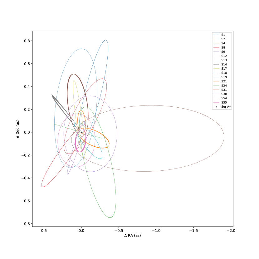
Figure 1: The fitted orbits of the 17 S-stars orbiting around Sgr A* with the best-fit values of orbital parameters from MCMC analysis.

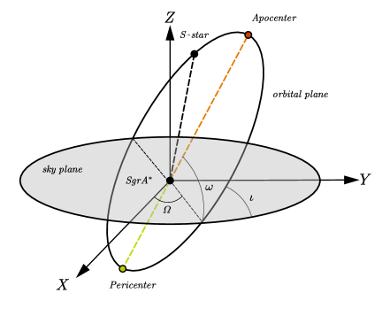
Figure 2: This figure illustrates the coordinate system we used for describing the orbits of stellar stars in the galactic center. The $Z$-axis follows the direction the Solar system points to the galactic center and the X-axis points east and the Y-axis points north. $\omega$ is the pericenter argument, $\Omega$ is the longitude of ascending node, and $\iota$ is the orbital inclination of the precessing elliptical orbit for S-stars.

Next, we need to solve the time delay problem to obtain the correct positions of the stars. The Romer time delay is the main consideration in this work, which can be expressed as:

$$t_{\rm{obs}}-t_{\rm{em}}=\frac{Z(t_{\rm{em}})}{c},$$ (52)

where $c$ is the speed of light. Using the equations (17), (18), (19), (29), and (35), one can get the positions on the orbital plane and the corresponding emission time of light. Projecting these theoretical positions onto the sky plane using the Thiele-Innes constants (given by equations (46, 47, 48, 49, 50, 51)) and solving for the Romer time delay, one obtains the projection onto the sky plane of the theoretical positions in the quantum-extended Schwarzschild spacetime $\left(X_{\rm{LQG}}(t_{\rm{obs}}),Y_{\rm{LQG}}(t_{\rm{obs}})\right)$.

III.2 Dataset of velocity and analysis

The velocity dataset includes the radial velocity and its corresponding observational time. It is important to consider the photon’s frequency shift, denoted as $\zeta$, which affects the radial velocity. This shift can be expressed as

$$\zeta=\frac{\Delta\nu}{\nu}=\frac{\nu_{\rm em}-\nu_{\rm obs}}{\nu_{\rm obs}}=\frac{V_{\rm R}}{c},$$ (53)

where $\nu_{\rm em}$ is the frequency of the photon at the time of emission, $\nu_{\rm obs}$ is the frequency when it is observed, and $V_{\rm R}$ is the radial velocity of the S-stars.

In our analysis of the photon’s frequency shift, we focus on two relativistic effects: the Doppler shift $\zeta_{\rm D}$ and the gravitational shift $\zeta_{G}$. These are defined as follows:

$$\zeta_{\rm D} = \frac{\sqrt{1-\frac{v_{\rm em}^{2}}{c^{2}}}}{1-\bm{n}\cdot\bm{v}_{\rm em}},$$ (54)

$$\zeta_{\rm G} = \frac{1}{\sqrt{1-\frac{2M}{r\left(\frac{M}{2r}+1\right)^{2}}+\frac{6A_{\lambda}M^{2}}{r^{2}\left(\frac{M}{2r}+1\right)^{4}}}},$$ (55)

where $v_{\rm em}$ is the velocity at the time of emission, and $\bm{n}\cdot\bm{v}_{\rm em}$ is the Newtonian line-of-sight velocity. One can then obtain the total frequency shift $\zeta$ as:

$$\zeta=\zeta_{\rm D}\cdot\zeta_{\rm G}-1.$$ (56)

III.3 Orbital precession of S2

The GRAVITY Collaboration has successfully measured the orbital precession of S2 per orbit, as reported in GRAVITY2 . The measured value is given by

$$\Delta\phi_{\rm per\;orbit}=12.1\times(1.10\pm 0.19).$$ (57)

Different from the measurement of S2’s orbit by only using the data of positions and velocities of S2 stars, the measurement of the orbital procession of S2 has used a large amount of new data, as mentioned clearly in GRAVITY2 . Thus in this paper, we treat this result as an independent measurement and use it independently in our analysis. This above orbital precession is an important phenomenon that cannot be explained by the Keplerian orbit under Newtonian gravity, as shown in (42). In addition to the effects of classical gravity, the parameter $A_{\lambda}$ arising from the quantum-extended Schwarzschild spacetime also contributes to the pericenter precession. Therefore, we can use the measured precession of S2 per orbit to constrain $A_{\lambda}$ from an MCMC analysis.

IV Analysis of Monte Carlo Markov Chain

In this section, we perform the analysis of MCMC by open-source emcee package in Python to obtain the constraints of $A_{\lambda}$ in the quantum-extended Schwarzschild spacetime. We The parameter space we explored through the MCMC analysis are summarized below

$$\{M,R,a,e,i,\omega,\Omega,T_{\rm P},x_{0},y_{0},v_{x_{0}},v_{y_{0}},v_{z_{0}},A_{\lambda}\},$$ (58)

where $M$ is the mass of the central black hole in Sgr A* and $R$ is the distance between the Earth and the black hole, $T_{\rm p}$ refers to the time of the pericenter of the osculating elliptical orbit, which we choose as the starting point of the calculation. $\{a,e,\iota,\omega,\Omega\}$ are the five orbital elements that describe the osculating elliptical orbits of each S-star. The parameters $\{x_{0},y_{0},v_{x_{0}},v_{y_{0}},v_{z_{0}}\}$ represent the zero-point offsets and drifts of the reference frame’s center.

To ensure that the parameters are not biased by the choice of priors, we choose to use uniform priors for all parameters. The range of the priors is based on previous results in Mon , and we set the prior for $A_{\lambda}$ to be $[0,2]$. For the likelihood function $\mathcal{L}$, we use three parts: the positions, radial velocities, and orbital precession

$$\log{\cal L}=\log{\cal L}_{\rm P}+\log{\cal L}_{\rm VR}+\log{\cal L}_{\rm pre}.$$ (59)

Since the covariance matrix is not available from the public data we got, we do not consider correlations between data. Therefore, the likelihood of the positions, $\log{\cal L}_{\rm P}$, is defined as

$$\log{\cal L}_{\rm P}= - \frac{1}{2}\sum_{i}\frac{(X_{\rm data}^{i}-X_{\rm LQG}^{i})^{2}}{(\sigma^{i}_{X,{\rm data}})^{2}}$$ (60)

$$- \frac{1}{2}\sum_{i}\frac{(Y_{\rm data}^{i}-Y_{\rm LQG}^{i})^{2}}{(\sigma^{i}_{Y,{\rm data}})^{2}},$$

where $X_{\rm data}^{i}$ and $Y_{\rm data}^{i}$ are the measured positions of the star at time $i$, $X_{\rm LQG}^{i}$ and $Y_{\rm LQG}^{i}$ are the corresponding positions predicted by our model, and $\sigma^{i}_{X,{\rm data}}$ and $\sigma^{i}_{Y,{\rm data}}$ are the uncertainties in the measurements. The likelihood of the radial velocities, $\log{\cal L}_{\rm VR}$, is defined as

$$\log{\cal L}_{\rm VR}=\frac{1}{2}\sum_{i}\frac{(V_{\rm R,data}^{i}-V_{\rm R,LQG}^{i})^{2}}{(\sigma^{i}_{V_{\rm R,data}})^{2}},$$ (61)

where $V_{\rm R,data}^{i}$ is the measured radial velocity of the star at time $i$, $V_{\rm R,LQG}^{i}$ is the corresponding radial velocity predicted by our model, and $\sigma^{i}_{V_{\rm R,data}}$ is the uncertainty in the measurement. The likelihood of the orbital precession, $\log{\cal L}_{\rm pre}$, is defined as

$$\log{\cal L}_{\rm pre}=-\frac{1}{2}\frac{(\Delta\phi_{\rm data}-\Delta\phi_{\rm LQG})^{2}}{\sigma^{2}_{\Delta\phi,{\rm data}}},$$ (62)

where $\Delta\phi_{\rm data}$ is the measured orbital precession of S2 (57), $\Delta\phi_{\rm LQG}$ is the corresponding orbital precession predicted by our model with the given value of $A_{\lambda}$, and $\sigma^{2}_{\Delta\phi,{\rm data}}$ is the uncertainty in the measurement.

Since we only have the measurement of S2’ s orbital precession, $\log{\cal L}_{\rm pre}$ will only be used in the MCMC analysis of S2. By combining these likelihood functions, we can obtain the overall likelihood function $\log{\cal L}$ as defined in (59).

V Results

With all preparations made, we performed the MCMC analysis separately for each of the 17 S-stars to constrain the LQG parameter $A_{\lambda}$ in the quantum-extended Schwarzschild black hole. It is important to note that we only added the orbital precession likelihood to the MCMC analysis of S2, as it is the only star for which we have detected its orbital procession.

The results of the marginalized posterior distributions of the LQG parameter $A_{\lambda}$ from the analysis with all the 17 S-stars are presented in Fig. 3. The orange curve represents the result constrained by the data of S2, and the green curve represents the result constrained by the data of S4. We observe that only the data of S2 and S4 can lead to meaningful constraints on $A_{\lambda}$. By comparing the results from the data of S2 and S4, one observes that the constraint from S2 is stronger than that from S4. Therefore, we select the value constrained by the data of S2 to be the final bound on $A_{\lambda}$, which places an upper limit on $A_{\lambda}$,

$$A_{\lambda}\lesssim 0.302$$ (63)

at 95% confidence level. We also plot the marginalized posterior distributions of $A_{\lambda}$ from S2 in Figure 4. In this figure, the vertical dash line denotes the 90% upper limits of $A_{\lambda}$.

In Figures 5 and 6, we illustrate the full posterior distributions of our 14-dimensional parameter space of our orbital model for S2 and S4, respectively. On the contour plots of both figures, the shaded regions show the 68%, 90%, and 95% confidence levels of the posterior probability density distributions of the entire set of parameters, respectively.

As expected, the MCMC analysis shows that the data of S2 gives the best result due to its large data size and the inclusion of the measurements of the orbital precession. According to the principle of MCMC, larger data sizes can result in more accurate results, while the inclusion of the orbital precession can help break the degeneracy between the parameters $M,a,e,$ and $A_{\lambda}$ as shown by the precession per orbit function (42). However, it is important to note that the degeneracy could not be completely broken. Figure 5 displays contour maps that vary from circular to elliptical, indicating the presence of degeneracy between some parameters. In addition, we would like to mention here that in the above analysis, we perform MCMC analysis separately for each of the 17 S-stars. It is interesting to perform a global analysis with all 17 stars together, which is computationally expensive due to a large number of orbital parameters. We expect to come back to this issue in our future works.

Clearly, the result we obtained is not as strong as those obtained from observations on the scale of the solar system, such as the gravitational time delay measured by the Cassini mission or the perihelion precession of Mercury Liu:2022qiz . However, our result demonstrates that observations at the galactic center can provide constraints on black hole parameters beyond those predicted by GR. Our analysis offers a bound on the black hole parameter in the strong gravity regime, which differs from the constraints obtained from observations in our solar system.

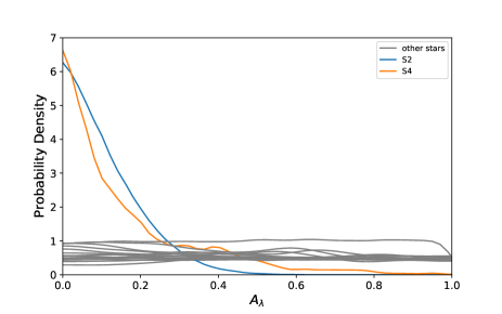
Figure 3: The marginalized posterior distributions of the LQG parameter $A_{\lambda}$ from the analysis with all the 17 S-stars. We performed kernel density estimation(KDE) on these data and show them in the same figure to compare the results. One can easily find out that only the data of S2 and S4 can be used to constrain $A_{\lambda}$ well.

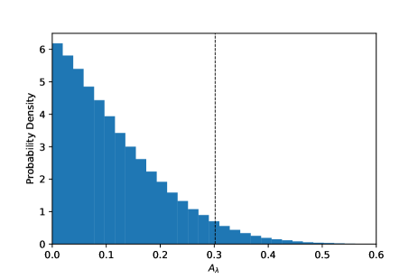
Figure 4: The constraint results of $A_{\lambda}$ by the data of S2, $A_{\lambda}<0.302$ at 95% confidence level. We extract the constraint results of $A_{\lambda}$ from fig 5 and use a bar chart to show its density distribution which looks like a half Gaussian distribution. One can see the peak value is $0$ which is consistent with the Schwarzschild result.

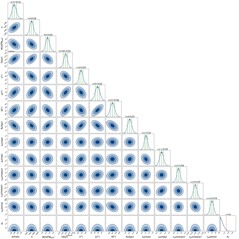
Figure 5: The posterior distribution of the orbital parameters of the S2 star and the LQG parameter $A_{\lambda}$ of the quantum-extended Schwarzschild black hole with uniform priors for all parameters. The LQG parameter $A_{\lambda}$ is constrained to be $A_{\lambda}<0.302$ at 95% confidence level.

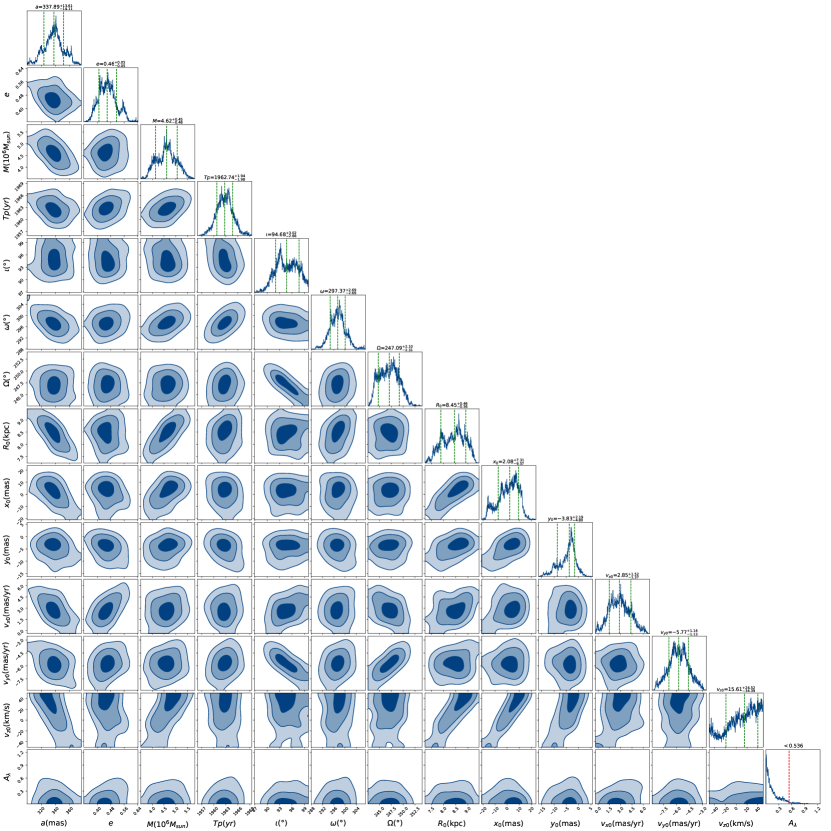
Figure 6: The posterior distribution of the orbital parameters of the S4 star and the LQG parameter $A_{\lambda}$ of the quantum-extended Schwarzschild black hole with uniform priors for all parameters. The LQG parameter $A_{\lambda}$ is constrained to be $A_{\lambda}<0.536$ at 95% confidence level.

VI conclusion

In this paper, we introduced the quantum-extended Schwarzschild spacetime and analyzed the motion of massive particles in this spacetime using the dynamics of perturbation. Our findings showed that the orbit of massive particles in this spacetime is a precessing ellipse, and the parameter $A_{\lambda}$ arising from the quantum-extended Schwarzschild spacetime affects the pericenter advance per orbit. To constrain the value of $A_{\lambda}$, we compared the effects of the quantum-extended of the Schwarzschild spacetime with publicly available data of 17 S-stars orbiting around Sgr A* in the central region of the Milky Way. We then carried out an MCMC analysis with all of this data.

To avoid the effects of degeneracy, we gave uniform priors for all 14 parameters. Additionally, based on the fact that S2 has the biggest data size and the most accurate data of precession, we expected S2 to give the most reliable result. As expected, S2 gave the best constraint result, with $A_{\lambda}<0.302$ at the 95% confidence level. It is also worth mentioning that we ignored the effects of the angular momentum of this spacetime since we expected the effects caused by rotation to be very small.

References

- (1) C. M. Will, The Confrontation be- tween General Relativity and Experiment, Living Rev. Relativ. 17, 4 (2014).
- (2) R. S. Park, W. M. Folkner, A. S. Konopliv, J. G. Williams, D. E. Smith, and M. T. Zuber, Precession of Mercury’s Perihelion from Ranging to the MESSENGER Spacecraft, Astrophys. J. 153, 121 (2017).
- (3) E. Fomalont, S. Kopeikin, G. Lanyi, and J. Benson, Progress in Measurements of the Gravitational Bending of Radio Waves Using the Vlba, Astrophys. J. 699, 1395 (2009).
- (4) B. Bertotti, L. Iess and P. Tortora, A test of general relativity using radio links with the Cassini spacecraft, Nature 425, 374 (2003).
- (5) I. H. Stairs, Testing General Relativity with Pulsar Timing, Living Rev. Rel. 6, 5 (2003).
- (6) N. Wex, Testing Relativistic Gravity with Radio Pulsars, [arXiv:1402.5594 [gr-qc]].
- (7) K. Akiyama et al. [Event Horizon Telescope Collaboration], First M87 Event Horizon Telescope Results. V. Physical Origin of the Asymmetric Ring, Astrophys. J. 875, L5 (2019).
- (8) K. Akiyama et al. [Event Horizon Telescope Collaboration], First M87 Event Horizon Telescope Results. VI. The Shadow and Mass of the Central Black Hole, Astrophys. J. 875, L6 (2019).
- (9) B. P. Abbott et al. [The LIGO Scientific Collab- oration and the Virgo Collaboration], Observa- tion of Gravitational Waves from a Binary Black Hole Merger, Phys. Rev. Lett. 116, 061102 (2016).
- (10) S. W. Hawking and G. F. R. Ellis, The Large Scale Struc- ture of Space-Time (Cambridge University Press, 1973).
- (11) A. Ashtekar, J. Olmedo, and P. Singh, Quantum extension of the Kruskal spacetime, Phys. Rev. D 98, 126003 (2018).
- (12) M. Bojowald, S. Brahma, and D.-H. Yeom, Effective line elements and black-hole models in canonical loop quantum gravity, Phys. Rev. D 98, 046015 (2018).
- (13) E. Alescia, S. Bahramia, D. Pranzetti, Quantum gravity predictions for black hole interior geometry, Phys. Lett. B 797, 134908 (2019).
- (14) M. Assanioussi, A. Dapor, and K. Liegener, Perspectives on the dynamics in a loop quantum gravity effective description of black hole interiors, Phys. Rev. D 101, 026002 (2020).
- (15) A. Perez, Black holes in loop quantum gravity, Rep. Prog. Phys. 80, 126901 (2017).
- (16) C. Rovelli, “Quantum gravity,” Cambridge University Press, Cambridge (2004).
- (17) T. Thiemann, “Modern Canonical Quantum General Relativity,” Cambridge University Press, 2007, ISBN 978-0-511-75568-2, 978-0-521-84263-1.
- (18) A. Ashtekar and J. Lewandowski, “Quantum theory of geometry. 1: Area operators,” Class. Quant. Grav. 14, A55-A82 (1997).
- (19) A. Ashtekar and J. Lewandowski,“Quantum theory of geometry. 2. Volume operators,” Adv. Theor. Math. Phys. 1, 388-429 (1998).
- (20) A. Ashtekar, T. Pawlowski and P. Singh,“Quantum Nature of the Big Bang: Improved dynamics,” Phys. Rev. D 74, 084003 (2006).
- (21) T. Thiemann, Quantum spin dynamics. VIII. The Master constraint, Class. Quant. Grav. 23, 2249-2266 (2006).
- (22) C. Rovelli, Black hole evolution traced out with Loop Quantum Gravity, APS Phys. 11, 127 (2018).
- (23) G. Ongole, H. Zhang, T. Zhu, A. Wang and B. Wang, Dirac Observables in the 4-Dimensional Phase Space of Ashtekar’s Variables and Spherically Symmetric Loop Quantum Black Holes, Universe 8, 543 (2022).
- (24) S. Hossenfelder, L. Modesto and I. Premont-Schwarz, Emission spectra of self-dual black holes, [arXiv:1202.0412 [gr-qc]].
- (25) S. Sahu, K. Lochan and D. Narasimha, Gravitational lensing by self-dual black holes in loop quantum gravity, Phys. Rev. D 91, 063001 (2015).
- (26) A. Ashtekar, J. Olmedo, and P. Singh, Quantum Transfiguration of Kruskal Black Holes, Phys. Rev. Lett. 121, 241301 (2018).
- (27) M. B. Cruz, C. A. S. Silva and F. A. Brito, Gravitational axial perturbations and quasinormal modes of loop quantum black holes, Eur. Phys. J. C 79, 157 (2019).
- (28) F. Caravelli and L. Modesto, Spinning Loop Black Holes, Class. Quant. Grav. 27, 245022 (2010).
- (29) M. Azreg-Aïnou, Comment on ’Spinning loop black holes’ , Class. Quant. Grav. 28, 148001 (2011).
- (30) J. M. Yan, Q. Wu, C. Liu, T. Zhu and A. Wang, Constraints on self-dual black hole in loop quantum gravity with S0-2 star in the galactic center, JCAP 09, 008 (2022).
- (31) T. Zhu and A. Wang, Observational tests of the self-dual spacetime in loop quantum gravity, Phys. Rev. D 102, 124042 (2020).
- (32) C. Liu, T. Zhu, Q. Wu, K. Jusufi, M. Jamil, M. Azreg-Aïnou and A. Wang, Shadow and quasinormal modes of a rotating loop quantum black hole, Phys. Rev. D 101, 084001 (2020).
- (33) Y. L. Liu, Z. Q. Feng and X. D. Zhang, Solar system constraints of a polymer black hole in loop quantum gravity, Phys. Rev. D 105, 084068 (2022).
- (34) Q. M. Fu and X. Zhang, Gravitational lensing by a black hole in effective loop quantum gravity, Phys. Rev. D 105, 064020 (2022).
- (35) Q. M. Fu and X. Zhang, Probing a polymerized black hole with the frequency shifts of photons, [arXiv:2212.11474 [gr-qc]].
- (36) A. Ashtekar, Black Hole evaporation: A Perspective from Loop Quantum Gravity, [arXiv:2001.08833].
- (37) W. C. Gan, N. O. Santos, F. W. Shu and A. Wang, Properties of the spherically symmetric polymer black holes, Phys. Rev. D 102, 124030 (2020).
- (38) A. Ashtekar and M. Bojowald, Quantum geometry and the Schwarzschild singularity, Class. Quant. Grav. 23, 391-411 (2006).
- (39) L. Modesto, Semiclassical loop quantum black hole, Int. J. Theor. Phys. 49, 1649-1683 (2010).
- (40) M. Assanioussi, A. Dapor and K. Liegener, Perspectives on the dynamics in a loop quantum gravity effective description of black hole interiors, Phys. Rev. D 101, 026002 (2020).
- (41) L. Modesto, Loop quantum black hole, Class. Quant. Grav. 23, 5587-5602 (2006).
- (42) A. Corichi and P. Singh, Loop quantization of the Schwarzschild interior revisited, Class. Quant. Grav. 33, 055006 (2016).
- (43) C. G. Boehmer and K. Vandersloot, Loop Quantum Dynamics of the Schwarzschild Interior, Phys. Rev. D 76, 104030 (2007).
- (44) W. C. Gan, X. M. Kuang, Z. H. Yang, Y. Gong, A. Wang and B. Wang, Non-existence of quantum black hole horizons in the improved dynamics approach, [arXiv:2212.14535 [gr-qc]].
- (45) W. C. Gan, G. Ongole, E. Alesci, Y. An, F. W. Shu and A. Wang, Understanding quantum black holes from quantum reduced loop gravity, Phys. Rev. D 106, 126013 (2022).
- (46) A. García-Quismondo and G. A. Mena Marugán, Two-time alternative to the Ashtekar-Olmedo-Singh black hole interior, Phys. Rev. D 106, 023532 (2022).
- (47) N. Bodendorfer, F. M. Mele and J. Münch, A note on the Hamiltonian as a polymerisation parameter, Class. Quant. Grav. 36, 187001 (2019).
- (48) N. Bodendorfer, F.M. Mele, and J. Münch, (b,v)-type variables for black to white hole transitions in effective loop quantum gravity, Phys. Lett. B 819, 136390 (2021).
- (49) N. Bodendorfer, F.M. Mele, and J. Münch, Effective quantum-extended spacetime of polymer Schwarzschild black hole, Class. Quant. Grav. 38, 095002 (2021).
- (50) S. Brahma, C. Y. Chen and D. h. Yeom, Testing Loop Quantum Gravity from Observational Consequences of Nonsingular Rotating Black Holes, Phys. Rev. Lett. 126, 181301 (2021).
- (51) T. Papanikolaou, Primordial black holes in loop quantum gravity: The effect on the threshold, [arXiv:2301.11439 [gr-qc]].
- (52) S. U. Islam, J. Kumar, R. Kumar Walia and S. G. Ghosh, Investigating Loop Quantum Gravity with Event Horizon Telescope Observations of the Effects of Rotating Black Holes, Astrophys. J. 943, 22 (2023).
- (53) M. Afrin, S. Vagnozzi and S. G. Ghosh, Tests of Loop Quantum Gravity from the Event Horizon Telescope Results of Sgr A∗, [arXiv:2209.12584 [gr-qc]].
- (54) S. Vagnozzi, R. Roy, Y. D. Tsai, L. Visinelli, M. Afrin, A. Allahyari, P. Bambhaniya, D. Dey, S. G. Ghosh and P. S. Joshi, et al. Horizon-scale tests of gravity theories and fundamental physics from the Event Horizon Telescope image of Sagittarius A∗, [arXiv:2205.07787 [gr-qc]].
- (55) R. Kumar Walia, Observational Predictions of LQG Motivated Polymerized Black Holes and Constraints From Sgr A* and M87*, [arXiv:2207.02106 [gr-qc]].
- (56) D. Pugliese and G. Montani, Constraining LQG Graph with Light Surfaces: Properties of BH Thermodynamics for Mini-Super-Space, Semi-Classical Polymeric BH, Entropy 22, 402 (2020).
- (57) T. Pawłowski, Observations on interfacing loop quantum gravity with cosmology, Phys. Rev. D 92, 124020 (2015).
- (58) D. Vaid, Quantum Hall Effect and Black Hole Entropy in Loop Quantum Gravity, [arXiv:1208.3335 [gr-qc]].
- (59) A. Barrau, T. Cailleteau, X. Cao, J. Diaz-Polo and J. Grain, Probing Loop Quantum Gravity with Evaporating Black Holes, Phys. Rev. Lett. 107, 251301 (2011).
- (60) L. Modesto and I. Premont-Schwarz, Self-dual Black Holes in LQG: Theory and Phenomenology, Phys. Rev. D 80, 064041 (2009).
- (61) R. Abuter et al. [GRAVITY], Detection of the Schwarzschild precession in the orbit of the star S2 near the Galactic centre massive black hole, Astron. Astrophys. 636, L5 (2020).
- (62) I. de Martino, R. della Monica and M. de Laurentis, f(R) gravity after the detection of the orbital precession of the S2 star around the Galactic Center massive black hole, Phys. Rev. D 104, L101502 (2021).
- (63) R. Della Monica, I. de Martino and M. de Laurentis, Orbital precession of the S2 star in Scalar–Tensor–Vector Gravity, Mon. Not. Roy. Astron. Soc. 510, 4757-4766 (2022).
- (64) R. Della Monica and I. de Martino, Unveiling the Nature of SgrA* with the Geodesic Motion of S-Stars, J. Cosmol. Astropart. Phys. 03, 007 (2022).
- (65) A. D’Addio, S-star dynamics through a Yukawa–like gravitational potential, Phys. Dark Univ. 33, 100871 (2021).
- (66) D. Psaltis, N. Wex and M. Kramer, A Quantitative Test of the No-Hair Theorem with Sgr A* using stars, pulsars, and the Event Horizon Telescope, Astrophys. J. 818, 121 (2016).
- (67) H. Qi, R. O. Shaughnessy, and P. Brady, Testing the black hole no-hair theorem with Galactic Center stellar orbits, Phys. Rev. D 103, 084006 (2021).
- (68) D. Benisty and A. C. Davis, Dark energy interactions near the Galactic Center, Phys. Rev. D 105, 024052 (2022).
- (69) P. C. Peters and J. Mathews, Gravitational radiation from point masses in a Keplerian orbit, Phys. Rev. 131, 435-439 (1963).
- (70) S. Gillessen, P. M. Plewa, F. Eisenhauer, R. Sari, I. Waisberg, M. Habibi, O. Pfuhl, E. George, J. Dexter, S. von Fellenberg, T. Ott, and R. Genzel, An Update on Monitoring Stellar Orbits in the Galactic Center, Astrophys. J. 837, 30 (2017).