Newton’s Third Law in the Framework of Special Relativity for Charged Bodies Part 3: Time Dependent Engines

Abstract

The Lorentz symmetry group entails physical equations whose solutions are retarded. This leads to the concept of a relativistic engine resulting from retardation of electromagnetic fields. We have shown that Newton’n third law cannot strictly hold in a distributed system, where the different parts are at a finite distance from each other and thus force imbalance is created at the system’s center of mass. As the system is affected by a total force for a finite period, mechanical momentum and energy are acquired by the system. In previous works we relied on the fact that the bodies were macroscopically natural. Lately we relaxed this assumption and studied charged bodies, thus analyzing the consequences on a possible electric relativistic engine. On the first paper on this subject we investigated this phenomena in general but gave an example of a system only at the stage of reaching a stationary state, a second paper was devoted to the same but on the atomic scale, here we shall analyze the charge relativistic engine in a general time dependent setting.
Keyword: Newton’s Third Law, Electromagnetism, Relativity

1 Introduction

Special relativity which is closely connected to the Lorentz symmetry group, was introduced in Einstein’s famous 1905 paper: ”On the Electrodynamics of Moving Bodies” [9]. This theory was a consequence of observations and the laws of electromagnetism, which were formulated in the nineteenth century by Maxwell in his famous equations [10, 11, 12] which owe their present form to Oliver Heaviside [13]. A consequence of Maxwell’s equations is that an electromagnetic signal travels at the speed of light $c$, and soon it was realized that light is an electromagnetic wave. Later Einstein [9, 11, 12] formulated the special theory of relativity, which postulates that the speed of light in vacuum $c$ is the maximal allowed speed. According to a prevalent interpretation of relativity, any object, signal or field can not travel faster than the speed of light in vacuum. Hence the phenomena of retardation, if at a distance $R$ from an observer a change is made, the observer will be ignorant of it for a time greater than $\frac{R}{c}$. Thus action and reaction cannot be generated simultaneously because of the signal speed.

Here we mention that the phenomena of retardation exist only in Lorentzian space-times [14, 15], those space-times are the only solutions for the case of empty or low density environments [16, 17]. However, in a limited region of space-time such as close to the big-bang [14] an Euclidean metric is possible, which does not enable retardation as is evident in the extreme homogeneity of the cosmic microwave background.

Newton’s laws of motion laid the foundation for classical mechanics. The three laws of motion were first compiled by Isaac Newton in his Philosophiae Naturalis Principia Mathematica (Mathematical Principles of Natural Philosophy), first published in 1687 [18, 19]. Although the first law is already mentioned in Philosophiae Principia by Descartes which was published in 1644. Here we shall be interested initially in the third law, which states: When one body exerts a force on a second body, the second body simultaneously exerts a force equal in magnitude and opposite in direction on the first body.

It follows from Newton’s third law, that the total sum of forces in a system which is not affected by external forces is null. This law has a significant number of experimental verifications and is thus one of the corner stones of physical sciences. However, it is easy to see that action and its reaction cannot be generated at exactly the same time because the speed of signal propagation is not infinite. Hence the third law cannot be correct in an exact sense, although it can be assumed valid for most practical applications due to high velocity of signal propagation. Thus the total sum of forces cannot be zero at every given time. Thus according to Newton’s second law: ”Force is equal to the rate of change of momentum. For a constant mass, force equals mass times acceleration”. A body must gain momentum, in the sense that it’s center of mass must be moving. Moreover, Newton’s first law states: ”every object will remain at rest or in uniform motion in a straight line unless compelled to change its state by the action of an external force”. However, as the body gains momenta due to the retardation phenomena it cannot continue to move on a straight line, hence the first law cannot be correct in an exact sense but only in an approximate sense.

In prevalent systems the above described motion is minute, but perhaps there is a way to make this motion significant, this line of thought lead to the concept of a relativistic engine.

Current locomotive systems are based on material parts; each gains momentum that is equal and opposite to the momentum of the other. A generic example is a rocket that sheds gas to move itself forward. However, retardation effects suggest a novel type of engine which is not composed of two material parts but of field and matter. Forgetting about the field, the material body seems to obtain momentum thus the total momentum increases violating the law of momentum conservation. However, it can be shown that the opposite amount of momentum is attributed to the field [4], thus the total momentum is indeed conserved. This is a result of Noether’s theorem which dictates that a system that possesses translational symmetry will conserve momentum. The total physical system composed of matter and field is indeed invariant under translations, while every part of the system (either matter or field) is not. Feynman [12] depicted two moving charges, apparently contradicting Newton’s third law as forces that the charges induce do not cancel (last part of 26-2), this is resolved in (27-6) in which it is noticed that the momentum gained by the two charge system is removed from the field momentum.

A relativistic engine is thus defined as a system in which its material center of mass is in motion due to the interaction of its material parts. Those may move with respect to each other or held in a rigid frame. This has no effect as we are interested in the motion of the center of mass only. We emphasize that a relativistic motor allows 3-axis motion (vertical motion included), it does not contain moving parts, it does not consume fuel (and does not emit carbon) it only consumes electromagnetic energy which may be supplied by solar panels or batteries. The relativistic engine is a perfect solution for space travel in which much of the space vehicle volume is devoted to fuel storage.

Griffiths & Heald [20] pointed out that the laws of Coulomb’s and Biot-Savart determine the electric and magnetic field configurations solely for static sources. Time-dependent generalizations of these laws described by Jefimenko [21] were used to study the applicability of Coulomb and Biot-Savart formulas outside the static domain. In an earlier paper, we made use of Jefimenko’s [21, 11] equation to study the force developing between two current loops [1]. This was later generalized to include the forces between a current carrying loop and a permanent magnet [2, 3]. Since the device is forced for a finite period, it will gain mechanical momentum and energy. The subject of momentum conversation was discussed in [4]. In [5, 6, 7, 8] the exchange of energy between the mechanical part of the relativistic engine and the electromagnetic field were discussed. In particular, it was shown that the total electromagnetic energy expenditure is six times the kinetic energy gained by the relativistic motor. It was also shown how some energy might be radiated from the relativistic engine device if the coils are not configured properly.

Previous works relied on the fact that the bodies were macroscopically natural, which means that the number of electrons and ions is equal in every volume element. In a later work [22] we relaxed this assumption and studied charged bodies, thus analysing the consequences of charge on a possible electric relativistic engine. Notice, however, that in the previous paper we only considered a relativistic engine reaching a stationary state while ignoring the possibility of engines which do not reach a stationary state as well as the transient stage of engines that do. The same criticism holds for a the second part of the same paper dealing with a relativistic engine on the atomic scale [23]. Here we make a more general analysis leading to a different kind of charged relativistic engine of a type that does not reach a stationary state.

2 Generated Momentum

According to Newton’s second law, a system with a non zero total force in its center of mass, must have a change in its total linear momentum $\vec{P}(t)$:

$$\vec{F}_{T}^{[2]}=\frac{d\vec{P}}{dt}$$ (1)

Assuming that $\vec{P}(-\infty)=0$ and also that there are not current or charge densities at $t=-\infty$, it follows from equation (81) of [22] that:

$$\vec{P}(t)=\frac{\mu_{0}}{4\pi}\int\int d^{3}x_{1}d^{3}x_{2}~{}\left[\frac{1}{2}\left(\rho_{2}\partial_{t}\rho_{1}-\rho_{1}\partial_{t}\rho_{2}\right)\hat{R}-(\rho_{1}\vec{J}_{2}+\rho_{2}\vec{J}_{1})R^{-1}\right]$$ (2)

Comparing equation (2) with the momentum gain of a non charged relativistic motor described by equation (64) of [4]:

$$\vec{P}_{mech}\cong\frac{\mu_{0}}{8\pi}\partial_{t}I_{1}(t)I_{2}(\frac{h}{c})^{2}\vec{K}_{122},\qquad\vec{K}_{122}=-\frac{1}{h^{2}}\oint\oint\hat{R}(d\vec{l}_{2}\cdot d\vec{l}_{1})$$ (3)

where $h$ is a typical scale of the system, $I_{1}(t)$ and $I_{2}$ are the currents flowing through two current loops and $d\vec{l}_{1},d\vec{l}_{2}$ are the current loop line elements. We notice some major differences. First, we notice a factor of $\left(\frac{h}{c}\right)^{2}$ in case of an uncharged motor. As, for any practical system the scale $h$ is of the order of one, this means that the charged relativistic motor is stronger than the uncharged motor by a factor of $c^{2}\sim 10^{17}$ which is quite a considerable factor. Second, we notice that for the uncharged motor, the current must be continuously increased in order to maintain the momentum in the same direction. Of course, one cannot do this for ever, hence the uncharged motor is a type of a piston engine doing a periodic motion backward and forward and can only produce motion forward by interacting with an external system (the road). This is not the case for the charged relativistic motor. In fact we obtain non vanishing momentum for stationary charge and current densities:

$$\vec{P}(t)=-\frac{\mu_{0}}{4\pi}\int\int d^{3}x_{1}d^{3}x_{2}~{}(\rho_{1}\vec{J}_{2}+\rho_{2}\vec{J}_{1})R^{-1}$$ (4)

hence the charged relativistic motor can produce forward momentum without interacting with any external system except the electromagnetic field.

3 Engine Optimization

At this stage we would like to investigate what are the conditions for a system in terms of composition and structure to generate a maximal amount of momentum. To this end we write the charge density and current density in the form:

$$\rho(\vec{x},t)=\bar{\rho}\sum_{n}\rho^{n}(\vec{x})f^{n}(t)$$ (5)

in which $\bar{\rho}$ is a constant which has the units of current density, $\rho^{n}(\vec{x})$ are spatial functions and $f^{n}(t)$ temporal functions, both functions are dimensionless. Similarly:

$$\vec{J}(\vec{x},t)=\bar{J}\sum_{n}\vec{J}^{n}(\vec{x})g^{n}(t)$$ (6)

in which $\bar{J}$ is a constant which has the units of current density, $\vec{J}^{n}(\vec{x})$ are spatial vector functions and $g^{n}(t)$ temporal functions, both functions are dimensionless. We shall write the dimensional constants in terms of a generic charge $Q$, typical length scale $h$, and typical time scale $\tau$, that is:

$$\bar{\rho}\equiv\frac{Q}{h^{3}},\qquad\bar{J}\equiv\bar{\rho}\frac{h}{\tau}=\frac{Q}{h^{2}\tau}.$$ (7)

Next we shall attribute an expansion of the type given in equation (5) and equation (6) to each of the subsystems introduced previously this is done by adding a subscript with the relevant subsystem number:

$$\rho_{1}(\vec{x},t)=\bar{\rho}_{1}\sum_{n}\rho_{1}^{n}(\vec{x})f^{n}(t),\qquad\rho_{2}(\vec{x},t)=\bar{\rho}_{2}\sum_{n}\rho_{2}^{n}(\vec{x})f^{n}(t).$$ (8)

$$\vec{J}_{1}(\vec{x},t)=\bar{J}_{1}\sum_{n}\vec{J}_{1}^{n}(\vec{x})g^{n}(t),\qquad\vec{J}_{2}(\vec{x},t)=\bar{J}_{2}\sum_{n}\vec{J}_{2}^{n}(\vec{x})g^{n}(t).$$ (9)

Next we define the following dimensionless vector constants:

$$\vec{\Gamma}^{mn}\equiv\vec{\Gamma}_{21}^{mn}\equiv\frac{1}{2h^{6}}\int d^{3}x_{1}d^{3}x_{2}\rho_{1}^{n}\rho_{2}^{m}\frac{\vec{x}_{1}-\vec{x}_{2}}{|\vec{x}_{1}-\vec{x}_{2}|}=-\vec{\Gamma}_{12}^{nm}$$ (10)

which depend on the spatial structure of the two charged systems. Similarly we define:

$$\vec{\Lambda}_{21}^{mn}\equiv\frac{1}{h^{5}}\int d^{3}x_{1}d^{3}x_{2}\frac{\rho_{2}^{m}\vec{J}_{1}^{n}}{|\vec{x}_{1}-\vec{x}_{2}|},\qquad\vec{\Lambda}_{12}^{mn}\equiv\frac{1}{h^{5}}\int d^{3}x_{1}d^{3}x_{2}\frac{\rho_{1}^{m}\vec{J}_{2}^{n}}{|\vec{x}_{1}-\vec{x}_{2}|},$$ (11)

we notice that generically:

$$\vec{\Lambda}_{21}^{mn}\neq\vec{\Lambda}_{12}^{mn},\qquad\vec{\Lambda}_{21}^{mn}\neq\vec{\Lambda}_{12}^{mn}.$$ (12)

Using the typical time scales of each of the systems $\tau_{1}$ and $\tau_{2}$ we define:

$$\vec{\Lambda}^{mn}\equiv\frac{1}{\tau_{1}+\tau_{2}}\left(\tau_{2}\vec{\Lambda}_{21}^{mn}+\tau_{1}\vec{\Lambda}_{12}^{mn}\right),\qquad\bar{\tau}=\frac{\tau_{1}\tau_{2}}{\tau_{1}+\tau_{2}}.$$ (13)

Plugging equation (8) and equation (9) into equation (2) and using the definitions above we arrive at the expression:

$$\vec{P}(t)=\frac{\mu_{0}}{4\pi}Q_{1}Q_{2}\sum_{mn}\left[\vec{\Gamma}^{mn}(f^{m}\partial_{t}f^{n}-f^{n}\partial_{t}f^{m})-\frac{1}{\bar{\tau}}\vec{\Lambda}^{mn}f^{m}g^{n}\right].$$ (14)

We remind the reader that $\rho$ and $\vec{J}$ are not independent as they are connected through the continuity equation (16) of [22]:

$$\vec{\nabla}\cdot\vec{J}+\partial_{t}\rho=0\Rightarrow\sum_{n}\left[\bar{\rho}\rho^{n}(\vec{x})\partial_{t}f^{n}(t)+\bar{J}\vec{\nabla}\cdot\vec{J}^{n}g^{n}(t)\right]=0.$$ (15)

Taking into account equation (7) it follows that:

$$\sum_{n}\left[\rho^{n}(\vec{x})\tau\partial_{t}f^{n}(t)+h\vec{\nabla}\cdot\vec{J}^{n}(\vec{x})g^{n}(t)\right]=0.$$ (16)

As we can always choose:

$$g^{n}(t)=\tau\partial_{t}f^{n}(t),$$ (17)

the following equation must be satisfied:

$$\sum_{n}\left[(\rho^{n}(\vec{x})+h\vec{\nabla}\cdot\vec{J}^{n}(\vec{x}))g^{n}(t)\right]=0.$$ (18)

One possible solution is by choosing:

$$\rho^{n}(\vec{x})=-h\vec{\nabla}\cdot\vec{J}^{n}(\vec{x}),$$ (19)

for all $n$. In this case we can choose $\vec{J}^{n}$ but $\rho^{n}$ are dictated.

4 General Considerations

Looking at the momentum equation (14) it is obvious that the higher the charge the higher the momentum, also a short time scale $\bar{\tau}$ and a high time derivative will also increase momentum. Counter intuitively a proximity of charge and currents is also a contributing factor, through the lambda terms given in equation (11) this can be explained due to the fact that interaction is stronger in close proximity despite the fact that retardation is smaller. In fact interaction increases in proportion to the inverse of the distance square as the systems become closer, however, retardation only decreases linearly in the distance. We remind the reader that in a previous paper [22] we have shown that the amount of charge in a given volume is limited due to the phenomenon of dielectric breakdown, hence to achieve high momentum one needs high charge and thus a large engine as expected.

5 Example

Let us consider a set of two functions:

$$f^{1}(t)=\sin\phi_{1}(t),\qquad f^{2}(t)=\sin\phi_{2}(t)$$ (20)

in which $\phi_{1}(t)$ and $\phi_{2}(t)$ are arbitrary time dependent phases. We use equation (17) to choose corresponding $g$ functions:

$$g^{1}(t)=\tau\dot{\phi}_{1}(t)\cos\phi_{1}(t),\qquad g^{2}(t)=\tau\dot{\phi}_{2}(t)\cos\phi_{2}(t).$$ (21)

We shall assume two sub systems each described by only one component in the sum:

$$\vec{J}_{1}(\vec{x},t)=\bar{J}_{1}\vec{J}_{1}^{1}(\vec{x})g^{1}(t),\qquad\vec{J}_{2}(\vec{x},t)=\bar{J}_{2}\vec{J}_{2}^{2}(\vec{x})g^{2}(t).$$ (22)

Taking into account equation (19) it follows that:

$$\rho_{1}(\vec{x},t)=\bar{\rho}_{1}\rho_{1}^{1}(\vec{x})f^{1}(t),\qquad\rho_{2}(\vec{x},t)=\bar{\rho}_{2}\rho_{2}^{2}(\vec{x})f^{2}(t).$$ (23)

Only the following terms in equation (10) and equation (11) are non zero:

$$\vec{\Gamma}^{21}=\frac{1}{2h^{6}}\int d^{3}x_{1}d^{3}x_{2}\rho_{1}^{1}\rho_{2}^{2}\frac{\vec{x}_{1}-\vec{x}_{2}}{|\vec{x}_{1}-\vec{x}_{2}|},$$ (24)

$$\vec{\Lambda}_{21}^{21}\equiv\frac{1}{h^{5}}\int d^{3}x_{1}d^{3}x_{2}\frac{\rho_{2}^{2}\vec{J}_{1}^{1}}{|\vec{x}_{1}-\vec{x}_{2}|},\qquad\vec{\Lambda}_{12}^{12}\equiv\frac{1}{h^{5}}\int d^{3}x_{1}d^{3}x_{2}\frac{\rho_{1}^{1}\vec{J}_{2}^{2}}{|\vec{x}_{1}-\vec{x}_{2}|}.$$ (25)

Assuming $\tau_{1}=\tau_{2}$ it follows from equation (13) that $\bar{\tau}=\frac{\tau_{1}}{2}$, we shall take $\tau=\bar{\tau}$. Also it follows from equation (13) that:

$$\vec{\Lambda}^{12}=\frac{1}{2}\vec{\Lambda}_{12}^{12},\qquad\vec{\Lambda}^{21}=\frac{1}{2}\vec{\Lambda}_{21}^{21}.$$ (26)

Inserting the above results in equation (14) will yield:

$$\vec{P}(t)=\frac{\mu_{0}}{4\pi}Q_{1}Q_{2}\left[\vec{\Gamma}^{21}(f^{2}\partial_{t}f^{1}-f^{1}\partial_{t}f^{2})-\frac{1}{\bar{\tau}}\vec{\Lambda}^{21}f^{2}g^{1}-\frac{1}{\bar{\tau}}\vec{\Lambda}^{12}f^{1}g^{2}\right].$$ (27)

Let us make the following assumptions. First: we assume that the phases differ by a constant value $\Delta\phi$. This means that the derivatives of the phases are the same. Taking into account equation (20) and equation (21) we thus obtain:

$$\vec{P}(t)=\frac{\mu_{0}}{4\pi}Q_{1}Q_{2}\dot{\phi}\left[\vec{\Gamma}^{21}\sin\Delta\phi-\vec{\Lambda}^{21}\sin\phi_{2}\cos\phi_{1}-\vec{\Lambda}^{12}\sin\phi_{1}\cos\phi_{2}\right].$$ (28)

The $\Gamma$ and $\Lambda$ constants are determined by the distribution of charges and currents. Let us consider two thin wires of current as depicted in figure 1.

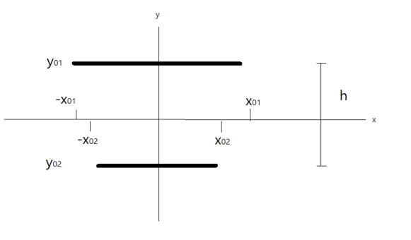
Figure 1: Two current strips.

In this case we obtain:

$$\vec{J}_{1}^{1} = h^{2}\delta(z_{1})\delta(y_{1}-y_{01})\left[u(x_{1}+x_{01})-u(x_{1}-x_{01})\right]\hat{x},$$

$$\vec{J}_{2}^{2} = h^{2}\delta(z_{2})\delta(y_{2}-y_{02})\left[u(x_{2}+x_{02})-u(x_{2}-x_{02})\right]\hat{x}.$$ (29)

in which $\delta$ is Dirac’s delta function and $u$ is a step function, $\hat{x}$ is a unit vector in the $x$ direction. It follows from equation (19) that we also have:

$$\rho_{1}^{1} = h^{3}\delta(z_{1})\delta(y_{1}-y_{01})\left[\delta(x_{1}-x_{01})-\delta(x_{1}+x_{01})\right],$$

$$\rho_{2}^{2} = h^{3}\delta(z_{2})\delta(y_{2}-y_{02})\left[\delta(x_{2}-x_{02})-\delta(x_{2}+x_{02})\right].$$ (30)

we shall take the characteristic length of the system to be the distance between the two wires (see figure 1):

$$h=y_{02}-y_{01}.$$ (31)

Now, we can plug equation (30) into equation (24) and obtain:

$$\vec{\Gamma}^{21}=h\hat{y}\left\{\frac{1}{\sqrt{(x_{01}+x_{02})^{2}+h^{2}}}-\frac{1}{\sqrt{(x_{01}-x_{02})^{2}+h^{2}}}\right\},$$ (32)

For the simple case: of $x_{01}=x_{02}$, it follows that for a wire of length $L=2x_{01}=x_{01}+x_{02}$, it takes the form:

$$\vec{\Gamma}^{21}=\hat{y}\left\{\frac{1}{(\sqrt{(\frac{L}{h})^{2}+1}}.-1\right\},$$ (33)

Thus if the wires is very long with respect to the distance between wires, $L\gg h$ it follows that:

$$\vec{\Gamma}^{21}=-\hat{y}.$$ (34)

For a vanishing short wire $\vec{\Gamma}^{21}=0$, while for a short wire $L\ll h$, we have:

$$\vec{\Gamma}^{21}=-\frac{1}{2}(\frac{L}{h})^{2}\hat{y}.$$ (35)

The absolute value of $|\Gamma^{21}|$ is depicted in figure 2:

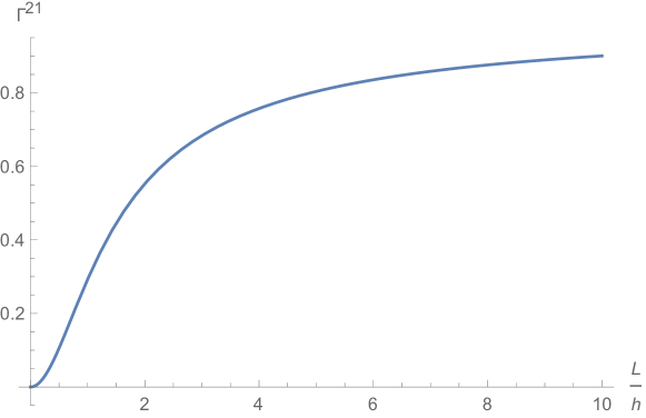
Figure 2: $|\Gamma^{21}|$, the functions approached asymptotically to a unit value.

Let us now insert equation (29) and equation (30) into equation (25) and equation (26) its follows that:

$$\Lambda_{12}^{12}=\Lambda_{21}^{21}=0\quad\Rightarrow\quad\vec{\Lambda}^{12}=\vec{\Lambda}^{21}=0.$$ (36)

Thus according to equation (28):

$$\vec{P}(t)=\frac{\mu_{0}}{4\pi}Q_{1}Q_{2}\dot{\phi}\vec{\Gamma}^{21}\sin\Delta\phi.$$ (37)

Assuming $\Delta\phi=\frac{\pi}{2}$ and a long enough wire:

$$\vec{P}(t)=-\frac{\mu_{0}}{4\pi}Q_{1}Q_{2}\dot{\phi}\hat{y}.$$ (38)

Hence, such a system will gain momentum in the $y$ direction (perpendicular to the wire direction) depending on the phase temporal derivative. The total current flowing through the wire (say wire 1) is:

$$I_{1}(t)=\int\vec{J}_{1}\cdot\hat{x}dydz=Q_{1}\dot{\phi}\cos\phi_{1},\qquad-x_{01}<x<+x_{01}$$ (39)

If we take $\phi_{1}=\omega t$:

$$I_{1}(t)=Q_{1}\omega\cos(\omega t)$$ (40)

which is the current that is needed to charge and discharge the ends of the wire. The amplitude of the said current is:

$$I_{a1}=Q_{1}\omega.$$ (41)

From equation (20), equation (23) and equation (30) it follows that the total charge in the wire is null because the charge accumulated in one end is equal and opposite to the other end with a maximal value of $Q_{1}$. The same goes of course in the case of wire 2. Thus we may write the momentum equation as:

$$\vec{P}(t)=-\frac{\mu_{0}}{4\pi\omega}I_{a1}I_{a2}\hat{y}.$$ (42)

6 Discussion

In this paper, we have shown that, in general, Newton’s third law is not compatible with the principles of special relativity and the total force on a two charged body system is not zero. Still, momentum is conserved if one takes the field momentum into account, and the same is true for energy.

The main results of this paper are given by equation (42), which describe the total relativistic force for a specific configuration. Although more general configurations are allowed (see equation (14)).

The result shows that the higher the current amplitude and counterintuitive the lower the frequency, the higher the momentum obtained. This is somewhat misleading because if the frequency is too low one may risk an aerial discharge (see discussion in [22]). However, neglecting this problem we obtain for two wires carrying a 10 kiloampere current, with 1 Hz frequency a momentum of 1.6 kg meter/second.

We remark that an ”antigravity” effect may be obtain by changing the phase quadratically in time, this will cause a second derivative of phase that may cause a temporal first derivative of momentum, i.e. a force.

Obviously to conduct an experimental verification of the suggested relativistic engine is highly desirable in order to corroborate the ideas presented in the current paper this is also left as a task for the future.

7 Conclusion

To conclude we make a comparison between the relativistic motor and other types of electromagnetic engines. A photon engine will emit photons backwards and thus propel itself forward. It may be a powerful laser or a radio-frequency cavity [24] (the only difference between those too cases are the energy and momenta of a single photon). To reach a momentum $p$ using a photon engine one needs an energy of $E_{p}=pc$ while for a relativistic engine an energy of $E\sim\frac{1}{2}pv$ will suffice. The ratio is $\frac{E_{p}}{E}=\frac{2c}{v}$ which is a huge number for non relativistic speeds.

Of course standard electric cars to today (Tesla for example) can reach significant speed and momentum, but unlike the relativistic motor they need a road to push against, otherwise no motion is possible.

References

- [1] Miron Tuval & Asher Yahalom ”Newton’s Third Law in the Framework of Special Relativity” Eur. Phys. J. Plus (11 Nov 2014) 129: 240 DOI: 10.1140/epjp/i2014-14240-x. (arXiv:1302.2537 [physics.gen-ph]).
- [2] Miron Tuval and Asher Yahalom ”A Permanent Magnet Relativistic Engine” Proceedings of the Ninth International Conference on Materials Technologies and Modeling (MMT-2016) Ariel University, Ariel, Israel, July 25-29, 2016.
- [3] Asher Yahalom ”Retardation in Special Relativity and the Design of a Relativistic Motor”. Acta Physica Polonica A, Vol. 131 (2017) No. 5, 1285-1288. DOI: 10.12693/APhysPolA.131.1285
- [4] Miron Tuval and Asher Yahalom ”Momentum Conservation in a Relativistic Engine” Eur. Phys. J. Plus (2016) 131: 374. DOI: 10.1140/epjp/i2016-16374-1
- [5] A. Yahalom ”Preliminary Energy Considerations in a Relativistic Engine” Proceedings of the Israeli-Russian Bi-National Workshop, page 203-213, 28-31 August 2017, Ariel, Israel.
- [6] S. Rajput and A. Yahalom, ”Preliminary Magnetic Energy Considerations in a Relativistic Engine: Mutual Inductance vs. Kinetic Terms” 2018 IEEE International Conference on the Science of Electrical Engineering in Israel (ICSEE), Eilat, Israel, 2018, pp. 1-5. doi: 10.1109/ICSEE.2018.8646265
- [7] S. Rajput and A. Yahalom, ”Material Engineering and Design of a Relativistic Engine: How to Avoid Radiation Losses”. Advanced Engineering Forum ISSN: 2234-991X, Vol. 36, pp 126-131. Submitted: 2019-06-16, Accepted: 2020-05-18, Online: 2020-06-17. ©2020 Trans Tech Publications Ltd, Switzerland.
- [8] Shailendra Rajput, Asher Yahalom & Hong Qin ”Lorentz Symmetry Group, Retardation and Energy Transformations in a Relativistic Engine” Symmetry 2021, 13, 420. https://doi.org/10.3390/sym13030420.
- [9] A. Einstein, ”On the Electrodynamics of Moving Bodies”, Annalen der Physik 17 (10): 891-921, (1905).
- [10] J.C. Maxwell, ”A dynamical theory of the electromagnetic field” Philosophical Transactions of the Royal Society of London 155: 459-512 (1865).
- [11] J. D. Jackson, Classical Electrodynamics, Third Edition. Wiley: New York, (1999).
- [12] R. P. Feynman, R. B. Leighton & M. L. Sands, Feynman Lectures on Physics, Basic Books; revised 50th anniversary edition (2011).
- [13] O. Heaviside, ”On the Electromagnetic Effects due to the Motion of Electrification through a Dielectric” Philosophical Magazine, (1889).
- [14] Yahalom, Asher. 2022. ”The Primordial Particle Accelerator of the Cosmos” Universe 8, no. 11: 594. https://doi.org/10.3390/universe8110594 arXiv:2211.09674 [gr-qc].
- [15] Yahalom, A. (2013). Gravity and Faster than Light Particles, Journal of Modern Physics (JMP), Vol. 4 No. 10 PP. 1412-1416. DOI: 10.4236/jmp.2013.410169.
- [16] A. Yahalom ”The Geometrical Meaning of Time” Foundations of Physics, Volume 38, Number 6, Pages 489-497 (June 2008). [”The Linear Stability of Lorentzian Space-Time” Los-Alamos Archives - gr-qc/0602034, gr-qc/0611124]
- [17] A. Yahalom ”The Gravitational Origin of the Distinction between Space and Time” International Journal of Modern Physics D, Vol. 18, Issue: 14, pp. 2155-2158 (2009).
- [18] I. Newton, Philosophiae Naturalis Principia Mathematica (1687).
- [19] H. Goldstein , C. P. Poole Jr. & J. L. Safko, Classical Mechanics, Pearson; 3 edition (2001).
- [20] D. J. Griffiths & M. A. Heald, ”Time dependent generalizations of the Biot-Savart and Coulomb laws” American Journal of Physics, 59, 111-117 (1991), DOI:http://dx.doi.org/10.1119/1.16589
- [21] Jefimenko, O. D., Electricity and Magnetism, Appleton-Century Crofts, New York (1966); 2nd edition, Electret Scientific, Star City, WV (1989).
- [22] Rajput, Shailendra, and Asher Yahalom. 2021. ”Newton’s Third Law in the Framework of Special Relativity for Charged Bodies” Symmetry 13, no. 7: 1250. https://doi.org/10.3390/sym13071250
- [23] Yahalom, Asher. 2022. ”Newton’s Third Law in the Framework of Special Relativity for Charged Bodies Part 2: Preliminary Analysis of a Nano Relativistic Motor” Symmetry 14, no. 1: 94.
- [24] Harold White, Paul March, James Lawrence, Jerry Vera, Andre Sylvester, David Brady and Paul Bailey, Measurement of Impulsive Thrust from a Closed Radio-Frequency Cavity in Vacuum, Journal of Propulsion and Power, Vol. 33, No. 4, July-August 2017.