Abstract

This paper aims to study the traversable wormhole models with two different shape functions within the context of Finsler geometry. By taking into account the anisotropic energy-momentum tensor, also we have examined the wormhole solution of the gravitational field equation in the framework of Finsler space-time and analyzed the validity of the solution of the Finsler wormhole by considering null energy, strong energy, weak energy, and dominant energy condition. Furthermore, we analyze the anisotropic factor to find out the nature of the gravity of the wormhole.

1 Introduction

A wormhole (WH) has a tube-like geometric structure that is asymptotically flat on both sides. These are hypothetical passages that associate two different regions of space-time. For the first time in 1935, Einstein and Rosen gave mathematical evidence for the existence of these hypothetical passages, and these passages are popularly known as Einstein–Rosen bridges [1]. The concept of WH was first brought by Flamm [2]. Misner and Wheeler later made the first use of the phrase “wormhole” [3]. Although WH models in General relativity (GR) call for the existence of exotic matter, it is now recognized that they can also occur in modified gravity theories with ordinary matter [4, 5]. The radius of the throat of the WH can be thought of as either fixed in the case of static wormholes (SWHs) or variable in the case of non-static or cosmic WHs [1].

WHs and black holes are special types of solutions to GR and arise when the structure of space-time is strongly dented by gravity. Proof for the existence of black holes has already been discussed in [6, 7]. On the other hand, proof of the existence of WH is still a big question. However, according to the GR, they might be possible, but that doesn’t mean they have to exist. But they are theoretically possible, and there are different kinds. And this has been deeply discussed in [8]. According to [9, 10], there is a possibility for the existence WHs in the galactic halo region. Gravitational lensing by WHs has been studied in [11, 12, 13].

It is well known that WHs offer a feasible technique for quick interstellar travel. They are the solution to Einstein’s field equations and link two far-off cosmological locations. A traversable WH was first introduced, by Morris and Thorne [14]. They examined spherically symmetric static objects using GR and demonstrated that they must violate energy conditions. Exotic matter in this energy-violating situation possesses physical characteristics which would violate laws of physics, which includes particles with a negative mass. WHs are a tremendously intriguing issue in theoretical physics because of these exceptional characteristics [15, 16, 17].

It has been proven that modified theories of gravity can significantly reduce or even eliminate the need for exotic matter. The birth of the dark universe theory has brought the constraints of GR into a wider view. Because of this, GR needs to be modified over vast distances and throughout the cosmos. Numerous initiatives have been made to learn more about the mechanism behind this increased proliferation. Recently, modifying GR on cosmological scales has attracted a lot of attention from researchers. To demonstrate this process, a variety of scholars have been put forth in the literature, ranging from the dark energy models to the modified gravitation theories. The higher-order curvature theories of gravity have gained a lot of attention recently due to their potential for producing cosmological models that can address the problem of the expanding universe. Astrophysicists have been interested in $f(R)$ modified gravity, where $R$ is the curvature scalar, as a way to reveal cosmic acceleration and develop several interesting hypotheses. A thorough presentation of the notable advancements in modified gravity during the previous few decades was offered by Clifton et al. [18].

T. Harko and colleagues presented an expansion of the $f(R)$ theories of gravity mentioned above by including the energy-momentum tensor trace $T$ as well as a general dependency on the Ricci scalar $R$ in the model’s gravitational action, known as the $f(R,T)$ gravity [19]. In fields including cosmology, thermodynamics, gravitational waves, and astrophysics, this alternative gravity hypothesis has been tested [20] - [23]. Despite these attempts, WHs in $f(R,T)$ gravity theories still have a low information content. A specific instance of the static wormhole (SWH) geometry was explored, in which its redshift function is independent of both time and spatial coordinates [24, 25]. Since the $T$ dependency in the $f(R,T)$ gravity appears from the inclusion of quantum processes, it could be fascinating to examine more generic WH theories.
Although no observational evidence of WHs has been discovered to date, some significant contributions in this area have lately been made. For instance, researchers examined the possibility of WHs in the galactic halo regions. It was established that a galactic halo’s space-time can be modeled by a traversable WH geometry that fits with the known flat galactic rotation curve. Further research into this matter revealed that gravitational lensing presents a strong prospect for the identification of these WHs [26]. Thin accretion disks around static spherically symmetric WHs were found to have distinctive signatures in the electromagnetic spectrum, thereby giving rise to the feasibility of differentiating WH geometries by astrophysical studies of such emission spectra [27, 28]. The majority of supermassive black hole contenders at the central region of galaxies may have originated as WHs in the early Universe. WHs with orbiting hot spots and black holes can be distinguished from one another using Einstein-ring systems [29, 30]. A WH may be a continuous ring-like structure that resembles a black hole, as demonstrated by R.A. Konoplya and A. Zhidenko [31].

Finsler geometry has drawn the attention of many physicists in recent years due to its ability to explain several problems that Einstein’s gravity is unable to explain. Riemannian geometry is a special case of Finsler geometry. When general relativity did not fully explain the behavior of gravity, research into gravitation theories on the basis of Finsler geometry began. GR is currently being used to explain a wide range of facts with remarkable precision. This theory faces few drawbacks in bulk and negligible scales [32]. The Finslerian framework extends GR without altering the dimension of space-time, making it more suitable to simultaneously explain observers, gravity, and causal structure [33]. Instead of changing the action of GR, Finslerian gravity theory is constructed by changing the geometric structure of the equations. The Finslerian space-time geometry is defined by a function on the tangent bundle rather than a base manifold. Finslerian space-time geometry benefits from these characteristics. The investigation of modified dispersion relations within the geometry of Finslerian space-time yields results that are consistent with recent experimental observations [34]. Studies of Finsler-Lagrange-Hamilton geometry and Finsler cosmological models can be found in [35] and [36]. Also, Quantum gravity benefits greatly from Finslerian space-time geometry. Experimental findings and current conventional high-energy theories are compatible with Finsler-like gravity theories. Without the dark matter hypothesis, Finsler geometry is a superior tool for addressing the problems with the experimental findings of spiral galaxies and their flat rotation curves [37].

Recently, H. M. Manjunatha and S.K. Narasimhamurthy studied the WH model in $f(R)$ gravity with exponential shape function within the Finsler geometry [38]. Also analyzed was the WH solution to the gravitational field within the context of an anisotropic energy-momentum tensor by adopting the Finslerian framework. With continuous progress in the discovery of WH efforts, it is essential to compile more predictions of their matter-geometry content. That is the objective of the current paper, in which we have studied the wormhole model considering polynomial shape function with the Finslerian approach in the perspective of the $f(R,T)$ theory of gravity. By considering the Modified gravitation theory i.e., $f(R,T)$ gravity, in the present article, we assume the function $f(R,T)=R+2f(T)$, where $f(T)=\lambda{T}$ and $R$, $T$, and $\lambda$ are the Ricci scalar, the Trace energy-momentum tensor, and a constant respectively. Based on these parameters, we construct different WH models and experimented with the violation of energy conditions with the help of graphs.

The paper is organized as follows. In section 2, we have discussed the Finslerian WH structure and its geometric formulations. In section 3, we derived the WH field equations in $f(R,T)$ gravity. In section 4, we constructed two different exact WH models from various hypotheses for their matter content, to be followed by a discussion on the violation of the energy conditions. Section 5 is devoted to a discussion and results. And finally, we conclude our article in section 6.

2 Finslerian Wormhole Structure

One needs to instigate the metric in order to search the WH structure. Let us assume that the Finsler structure has the following shape, [39].

$$F^{2}=B(r)y^{t}y^{t}-A(r)y^{r}y^{r}-r^{2}\bar{F^{2}}(\theta,\phi,y^{\theta},y^{\phi}).$$ (1)

Here, $B(r)=e^{2a(r)},$ where $a(r)$ is the red shift function and $A(r)=\left(1-\frac{b(r)}{r}\right)^{-1}$, where $b(r)$ represents the shape function of the WH, which must obey the following conditions.

• The radial coordinate $r$ lies between $r_{0}\leq r<\infty$, where $r_{0}$ is the throat radius of the WH metric.

• At the throat, $r=r_{0}$, then $b(r)$ satisfy the condition

  $$b(r_{0})=r_{0},$$ (2)

  and for the region outside the throat i.e., $r>r_{0}$,

  $$1-\frac{b(r)}{r}>0.$$ (3)

• $b(r)$ must satisfy the flaring out condition at the throat, i.e.,

  $$b^{\prime}(r_{0})<1,$$ (4)

  where “ ^′ ” = $d/dr$.

• For asymptotic flatness of the space-time geometry, the limit

  $$\frac{b(r)}{r}\rightarrow 0\quad as\quad|r|\rightarrow\infty,$$ (5)

  is required.

• $B(r)$ must be finite and non-vanishing at the throat $r_{0}$.
  With the reference [40, 41], we can consider $B(r)=k$, where $k$ is constant, to achieve the de Sitter and anti-de Sitter asymptotic behaviors. Since a constant redshift function can be absorbed in the normalized time coordinate, we take $B(r)=1$.
  

The above conditions signify the WH space-time geometry.

In this study, $\bar{F}$ is two-dimensional Finsler structure, and we consider $\bar{F^{2}}$ in the following form:

$$\bar{F}^{2}=y^{\theta}y^{\theta}+f(\theta,\phi)y^{\phi}y^{\phi}.$$ (6)

Thus

$$\bar{g}_{ij}=diag\left(1,f(\theta,\phi)\right),\quad\quad\bar{g}^{ij}=diag\left(1,\frac{1}{f(\theta,\phi)}\right),$$ (7)

where $i,j=\theta,\phi.$
We can calculate the geodesic spray coefficients

$$G^{\mu}=\frac{1}{4}g^{\mu\nu}\left(\frac{\partial^{2}F^{2}}{\partial{x^{\lambda}}\partial{y^{\nu}}}y^{\lambda}-\frac{\partial{F^{2}}}{\partial{x^{\nu}}}\right),$$ (8)

from $\bar{F^{2}}$ as

$$\bar{G^{\theta}}=-\frac{1}{4}\frac{\partial{f}}{\partial{\theta}}y^{\phi}y^{\phi},$$ (9)

$$\bar{G}^{\phi}=\frac{1}{4f}\left(2\frac{\partial{f}}{\partial{\theta}}y^{\phi}y^{\theta}+\frac{\partial{f}}{\partial{\phi}}y^{\phi}y^{\phi}\right).$$ (10)

from these we can obtain Ricci scalar $\bar{Ric}$:

$$\bar{Ric}=-\frac{1}{2f}\frac{\partial^{2}{f}}{\partial{\theta^{2}}}+\frac{1}{4f^{2}}\left(\frac{\partial{f}}{\partial{\theta}}\right)^{2},$$ (11)

which may be a constant or a function of $\theta$. For any constant value, say $\eta$, we can get the Finsler structure $\bar{F^{2}}$ in three different cases:

$$\bar{F}^{2}=\begin{cases}y^{\theta}y^{\theta}+A\sin^{2}(\sqrt{\eta}\theta)y^{\phi}y^{\phi},~{}~{}~{}~{}\eta>0\\ y^{\theta}y^{\theta}+A\theta^{2}y^{\phi}y^{\phi},~{}~{}~{}~{}~{}~{}~{}~{}~{}~{}~{}~{}~{}~{}~{}\eta=0\\ y^{\theta}y^{\theta}+A\sinh^{2}(\sqrt{-\eta}\theta)y^{\phi}y^{\phi}~{}~{}\eta<0.\end{cases}$$ (12)

Without loss of generality, we take $A=1$. Now the Finsler structure in Eq. (1) can be expressed as

$$F^{2}= \quad B(r)y^{t}y^{t}-A(r)y^{r}y^{r}-r^{2}y^{\theta}y^{\theta}-r^{2}\sin^{2}\theta y^{\phi}y^{\phi}$$ (13)

$$\quad+r^{2}\sin^{2}\theta y^{\phi}y^{\phi}-r^{2}\sin^{2}(\sqrt{\eta}\theta)y^{\phi}y^{\phi}.$$

That is,

$$F^{2}=\alpha^{2}+r^{2}\chi(\theta)y^{\phi}y^{\phi},$$ (14)

where $\chi(\theta)=\sin^{2}\theta-\sin^{2}(\sqrt{\eta}\theta)$ and $\alpha$ is Riemannian metric. Hence

$$F=\alpha\sqrt{1+\frac{r^{2}\chi(\theta)y^{\phi}y^{\phi}}{\alpha^{2}}}.$$ (15)

For the choice $b_{\phi}=r\sqrt{\chi(\theta)}$, we get

$$F=\alpha\phi(s),\quad\phi(s)=\sqrt{1+s^{2}},$$ (16)

where $s=\frac{b_{\phi}y^{\phi}}{\alpha}=\frac{\beta}{\alpha}$, $b_{\mu}=(0,0,0,b_{\phi})$, $b_{\phi}y^{\phi}$ = $b_{\mu}y^{\mu}=\beta$ ($\beta$ is $1$-form).

This indicates that $F$ is the metric $(\alpha,\beta)$ - Finsler space.
Isometric transformations of the Finsler structure [39] gives the Killing equation $K_{V}(F)=0$ in the Finsler space as follows:

$$\left(\phi(s)-s\frac{\partial\phi(s)}{\partial s}\right)K_{V}(\alpha)+\frac{\partial\phi(s)}{\partial s}K_{V}(\beta)=0$$ (17)

where

$$K_{V}(\alpha)= \ \frac{1}{2\alpha}(V_{\mu\mid\nu}+V_{\nu\mid\mu})y^{\mu}y^{\nu},$$ (18)

$$K_{V}(\beta)= \left(V^{\mu}\frac{\partial b_{\nu}}{\partial x^{\mu}}+b_{\mu}\frac{\partial V^{\mu}}{\partial x^{\nu}}\right)y^{\nu}.$$ (19)

Here “$\mid$” specifies the covariant derivative with respect to the Riemannian metric $\alpha$.
In the above consideration, we have $K_{V}(\alpha)+sK_{V}(\beta)=0$ or $\alpha K_{V}(\alpha)+\beta K_{V}(\beta)=0.$ This yields $K_{V}(\alpha)=0$ and $K_{V}(\beta)=0,$ or

$$V_{\mu\mid\nu}+V_{\nu\mid\mu}=0\quad\textrm{and}\quad V^{\mu}\frac{\partial b_{\nu}}{\partial x^{\mu}}+b_{\mu}\frac{\partial V^{\mu}}{\partial x^{\nu}}=0.$$

It is interesting to note that the first Killing equation of the Riemannian space is constrained by the second Killing equation. As a result, it is mainly responsible for shattering the Riemannian space’s isometric symmetry.

Actually, the current Finsler space for the case $\bar{F^{2}}$ as quadric in $y^{\theta}$ and $y^{\phi}$ can be obtained from the Riemannian manifold $(M,g_{\mu\nu}(x))$ as we have $F(x,y)=\sqrt{g_{\mu\nu}(x)y^{\mu}y^{\nu}}.$

Thus the gravitational field equations in the Finsler space can be obtained from the Einstein field equation in the Riemannian space-time with the metric Eq. (1) in which the metric $\bar{g}_{ij}$ is given by $\bar{g}_{ij}=diag(1,\sin^{2}\sqrt{\eta}\theta).$
That is, $g_{\mu\nu}=diag(B,-A,-r^{2},-r^{2}\sin^{2}\sqrt{\eta}\theta).$

Here the fresh parameter $\eta$ plays a significant role in the outcoming field equations in Finsler space and thereupon affects the Finsler geometric consideration of the WH problem.

The Finsler structure Eq. (1) gives geodesic spray coefficients:

$$G^{t} =0,$$ (20)

$$G^{r} =\frac{rb^{\prime}-b}{4r(r-b)}y^{r}y^{r}-\frac{r-b}{2}y^{\theta}y^{\theta}-\frac{r-b}{2}\sin^{2}(\sqrt{\eta}\theta)y^{\phi}y^{\phi},$$

$$G^{\theta} =\frac{1}{r}y^{r}y^{\theta}-\frac{\sqrt{\eta}}{2}\sin(\sqrt{\eta}\theta)\cos(\sqrt{\eta}\theta)y^{\phi}y^{\phi},$$

$$G^{\phi} =\frac{1}{r}y^{r}y^{\phi}+\sqrt{\eta}\cot(\sqrt{\eta}\theta)y^{\theta}y^{\phi}.$$

Now, we incorporate the geodesic spray coefficients from Eq. (20) into Eq. (11). Then we have

$$F^{2}Ric=\frac{rb^{\prime}-b}{r^{2}(r-b)}y^{r}y^{r}+\left(\eta-1+\frac{b}{2r}+\frac{b^{\prime}}{2}\right)y^{\theta}y^{\theta}$$ (21)

$$+\left(\eta-1+\frac{b}{2r}+\frac{b^{\prime}}{2}\right)\sin^{2}(\sqrt{\eta}\theta)y^{\phi}y^{\phi}.$$

We can define the scalar curvature in Finsler space as $S=g^{\mu\nu}Ric_{\mu\nu}$ and therefore, the Einstein-modified tensors in the Finsler space-time can be derived as

$$G_{\mu\nu}=Ric_{\mu\nu}-\frac{1}{2}g_{\mu\nu}S.$$ (22)

The constituents of Finsler modified Einstein tensor is obtained from Eq. (22) as follows:

$$G^{t}_{t} =\frac{1}{r^{2}}(b^{\prime}+\eta-1),$$ (23)

$$G^{r}_{r} =\frac{b}{r^{3}}+\frac{1}{r^{2}}(\eta-1),$$

$$G^{\theta}_{\theta} =G^{\phi}_{\phi}=\frac{rb^{\prime}-b}{2r^{3}}.$$

As the matter distribution for building a WH is still a demanding issue for the researchers, as a consequence, we consider the general anisotropic energy-momentum tensor [41] in the following form,

$$T^{\mu}_{\nu}=(\rho+p_{t})u^{\mu}u_{\nu}+(p_{r}-p_{t})\delta^{\mu}\delta_{\nu}-p_{t}g^{\mu}_{\nu},$$ (24)

where $\rho=\rho(r)$ is the energy density, $p_{r}=p_{r}(r)$ and $p_{t}=p_{t}(r)$ are radial and lateral (which is measured orthogonally to the radial direction) pressures, respectively. And $u^{\mu}$ the four-velocity such that $u^{\mu}u_{\mu}=1$, $\delta^{\mu}$ the space-like unit vector such that $\delta^{\mu}\delta_{\mu}=-1$ considered in the radial direction.
Adopting the above Finsler structure Eq. (1) and the stress-energy tensor Eq. (24), we can obtain the gravitational field equations in the Finsler geometry,

$$G^{\mu}_{\nu}=(8\pi_{F}+2\lambda)T^{i}_{j}+\lambda(-2\rho+T)g^{i}_{j},$$ (25)

where $4\pi_{F}$ stands for the volume of the Finsler space-time structure $\bar{F}$ in two-dimensions.
To obtain the gravitation field equations, we assume an anisotropic fluid obeying the matter content of the following form,

$$T^{\mu}_{\nu}=diag(\rho,-p_{r},-p_{t},-p_{t})$$ (26)

The trace $T$ of the energy momentum tensor appears to be $T=\rho-p_{r}-2p_{t}$.

3 Wormhole Field Equations in $f(R,T)$ Gravity

The constituents of the field equations Eq. (25) for the considered metric Eq. (13) with Eq. (26) are

$$G^{t}_{t} =(8\pi_{F}+\lambda)\rho-\lambda(p_{r}+2p_{t}):\hskip 56.9055pt\frac{1}{r^{2}}(b^{\prime}+\eta-1)=(8\pi_{F}+\lambda)\rho-\lambda(p_{r}+2p_{t}),$$ (27)

$$G^{r}_{r} =\lambda\rho+(8\pi_{F}+3\pi)p_{r}+2\lambda p_{t}:\hskip 54.06006pt-\frac{b}{r^{3}}-\frac{1}{r^{2}}(\eta-1)=\lambda\rho+(8\pi_{F}+3\pi)p_{r}+2\lambda p_{t},$$

$$G^{\theta}_{\theta} =G^{\phi}_{\phi}=\lambda\rho+\lambda p_{r}+(8\pi_{F}+\lambda)p_{t}:\hskip 36.98866pt\frac{b-rb^{\prime}}{2r^{3}}=\lambda\rho+\lambda p_{r}+(8\pi_{F}+\lambda)p_{t}.$$

The above set of field equations concede the solutions

$$\rho=\frac{b^{\prime}+(\eta-1)}{r^{2}(8\pi_{F}+2\lambda)},$$ (28)

$$p_{r}=-\frac{br+r(\eta-1)}{r^{3}(8\pi_{F}+2\lambda)},$$ (29)

$$p_{t}=\frac{b-b^{\prime}r}{2r^{3}(8\pi_{F}+2\lambda)}.$$ (30)

4 Wormhole Models

In the present section, we will obtain the models of WHs, which are constructed from various hypotheses for their matter content.

4.1 Model 1

In this model, we suppose the pressure $p_{t}$ and $p_{r}$ can be related as

$$p_{t}=np_{r},$$ (31)

with $n$ as an arbitrary constant. Such relations are taken in [42], for instance.
Using Eq. (31) in Eq. (29) and Eq. (30), we get

$$b(r)=(1-\eta)r+Ar^{1+2n},$$ (32)

where $A$ is an integration constant. Since the metric is asymptotically flat, the above equation Eq. (32) is stable when $n$ is negative and $A$ is positive. It also obeys the flaring-out condition.

The shape function $b(r)$ is plotted versus $r$ in Fig. (1) for the values $n=-0.4$ and $A=1$. And From such a figure, the basic WH condition, i.e., $b(r)<r$, is satisfied.

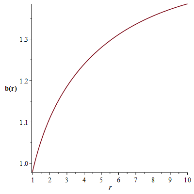
Figure 1: The shape function $b(r)$, with $A=1$, $\eta=1.01$, and $n=-0.4.$

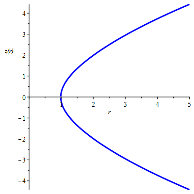
Figure 2: Nature of the shape function Eq. (32), at $r_{0}=1$

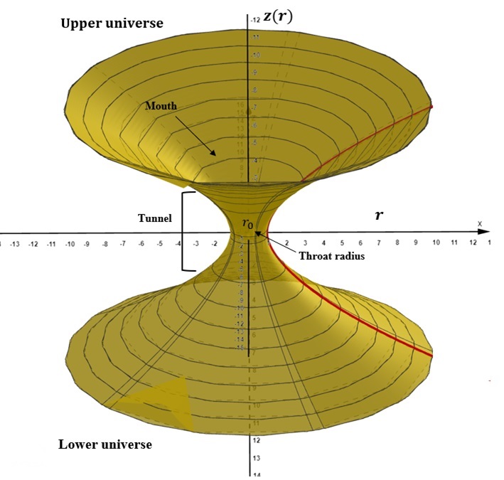
Figure 3: Embedded 3-D WH plot for the shape function Eq. (32)

The WH throat occurs at $r=r_{0}$ so that Eq. (2) gives

$$A=\frac{\eta}{r^{2n}_{0}}.$$ (33)

The energy density will be

$$\rho=\frac{(1+2n)A}{8\pi+2\lambda}r^{2(n-1)},$$ (34)

and the radial and lateral pressures given by

$$p_{r}=\frac{-A}{8\pi_{F}+2\lambda}r^{2(n-1)},$$ (35)

and

$$p_{t}=\frac{-nA}{8\pi_{F}+2\lambda}r^{2(n-1)}.$$ (36)

From Eqs. (34)-(36) we have

$$\rho+p_{r}=\frac{nA}{4\pi_{F}+\lambda}r^{2(n-1)},$$ (37)

$$\rho+p_{t}=\frac{A(1+n)}{8\pi_{F}+2\lambda}r^{2(n-1)}.$$ (38)

The presence of exotic matter in WHs violates the energy conditions. Accurately, the energy-momentum tensor violates the null energy condition (NEC) at the throat of the WH [43]. We can note from Eq. (37) the violation of NEC, i.e., $\rho+p_{r}\leq 0$, which intimates $\lambda>-4\pi$.

The dominant energy condition (DEC), $\rho\geq\lvert p_{r}\lvert$ and $\rho\geq\lvert p_{t}\lvert$, for this model is obtained from

$$\rho-p_{r}=\frac{A(1+n)}{4\pi_{F}+\lambda}r^{2(n-1)},$$ (39)

$$\rho-p_{t}=\frac{A(1+3n)}{8\pi_{F}+2\lambda}r^{2(n-1)}.$$ (40)

4.2 Model 2

In this model, we consider the matter along with the equation of the state (EoS)

$$p_{r}+\omega(r)\rho=0,$$ (41)

is stuffing the WH, for which $\omega(r)$ is a positive function of the radial coordinate. The same EoS with varying parameter $\omega(r)$ was considered in reference [44], for instance. Taking Eq. (41) in to account, from Eq. (28) and Eq. (29) we can get

$$\omega(r)=\frac{b+r(\eta-1)}{r(b^{\prime}+(\eta-1))}.$$ (42)

Further, we shall enquire about two cases for Eq. (42), as followed in [44].

Case I: $\omega(r)=\omega=\textrm{constant}$.
Which gives, from Eq. (42),

$$b(r)=(1-\eta)r+b_{0}r^{1/\omega},$$ (43)

where $b_{0}$ is an integrating constant. Since the metric is asymptotically flat, Eq. (43) is stable when $\omega>1$. Adopting some particular values of the parameters, we plot $b(r)$ in Fig. (4). It can be noticed that $r>r_{0}$ and $b(r)-r<0$ is an essential condition for the shape function to satisfy. $b(r)-r$ is also a decreasing function for $r>r_{0}$ which obeys the flaring out condition $b^{\prime}(r_{0})<1$.

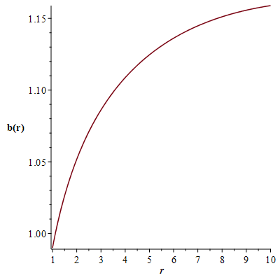
Figure 4: $b(r)$ with $\eta=1.01$, $b_{0}=1$, and $w=10$.

The WH throat occurs at $r=r_{0}$, that implies $b(r)=r_{0}$, which intimates

$$r_{0}=\left(\frac{b_{0}}{\eta}\right)^{\frac{\omega}{\omega-1}},$$ (44)

using Eq. (43) in Eqs. (28)-(30), we have

$$\quad\quad\quad\rho=\frac{-(\eta-1)r^{-2}\omega+b_{0}r^{\frac{1-3\omega}{\omega}}}{\omega(8\pi_{F}+2\lambda)},$$ (45)

$$~{}~{}~{}~{}~{}~{}p_{r}=\frac{(\eta-1)r^{-2}-b_{0}r^{\frac{1-3\omega}{\omega}}}{8\pi_{F}+2\lambda},$$ (46)

$$p_{t}=\frac{b_{0}(\omega-1)r^{\frac{1-3\omega}{\omega}}}{2\omega(8\pi_{F}+2\lambda)}.$$ (47)

NEC for this case is given by

$$\rho+p_{r}=\frac{b_{0}(1-\omega)r^{\frac{1-3\omega}{\omega}}}{\omega(8\pi_{F}+2\lambda)},~{}~{}~{}$$ (48)

$$~{}~{}~{}~{}~{}~{}~{}~{}~{}~{}~{}~{}~{}~{}~{}~{}~{}~{}~{}\rho+p_{t}=\frac{-2(\eta-1)r^{-2}\omega+b_{0}(1-\omega)r^{\frac{1-3\omega}{\omega}}}{2\omega(8\pi_{F}+2\lambda)},$$ (49)

from Eq. (48) the violation of NEC occurs for $b_{0}>0$ and $\lambda>-4\pi$. NEC for this case is presented in Fig. (5)-(6).

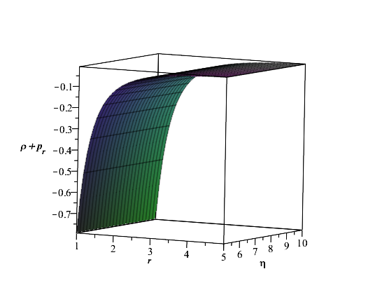
Figure 5: Violation of NEC, $\rho+p_{r}\leq 0$, with $b_{0}=1$, and $\lambda=-12$.

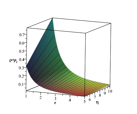
Figure 6: Validity region of NEC, $\rho+p_{t}\geq 0$, with $b_{0}=1$, and $\lambda=-18$.

DEC for this case is given by,

$$\rho-p_{r}=\frac{-2(\eta-1)r^{-2}\omega+b_{0}(1+\omega)r^{\frac{1-3\omega}{\omega}}}{\omega(8\pi_{F}+2\lambda)},$$ (50)

$$\rho-p_{t}=\frac{-2(\eta-1)r^{-2}\omega+b_{0}(3-\omega)r^{\frac{1-3\omega}{\omega}}}{2\omega(8\pi_{F}+2\lambda)}.$$ (51)

Those can be seen in Fig. (7)-(8).

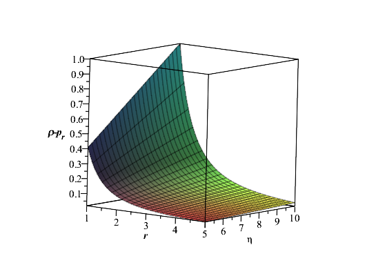
Figure 7: Validity region of DEC, $\rho\geq\lvert p_{r}\lvert$, with $b_{0}=1$, and $\lambda=-24$.

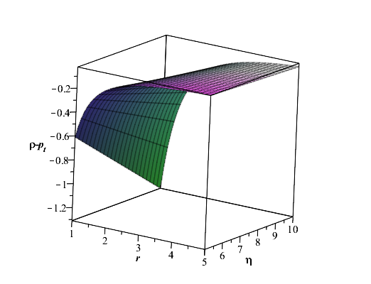
Figure 8: Validity region of DEC, $\rho\geq\lvert p_{t}\rvert$, with $b_{0}=1$, and $\lambda=-9$.

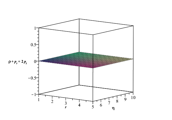
Figure 9: The SEC term: $\rho+p_{r}+2p_{t}=(\rho+p_{r}+2p_{t})(r,n)$ with $r_{0}=1$.

Case II: $\omega(r)=Br^{m}$

In this case, we assume $\omega(r)=Br^{m}$, where $B$ and $m$ are the positive constants. From the Eq. (42), the shape function now obtained as

$$b(r)=-r(\eta-1)+\exp{\left(c-\frac{1}{mBr^{m}}\right)},$$ (52)

where $c$ is the integration constant.

At the WH throat, we can have

$$c=\ln(\eta r_{0})+\frac{1}{mBr^{m}_{0}},$$ (53)

so Eq. (52) implies

$$b(r)=-r(\eta-1)+\exp{\left(\ln(\eta r_{0})+\frac{1}{mB}\left(\frac{1}{r^{m}_{0}}-\frac{1}{r^{m}}\right)\right)},$$ (54)

since $\omega>1$ and $m>0$, we have $r>r_{0}>(\frac{1}{B})^{(\frac{1}{m})}$, which obeys the asymptotically flatness condition of the metric. Hence the assumed EoS is justified. From Fig. (10), we can observe that when $r>r_{0}$, one can notice that $b(r)-r$ is decreasing function of $r$ for $r\geq r_{0}$ and $b^{\prime}(r_{0})<1$, which obeys the flaring out condition. Hence, the plotted shape function indeed expresses a WH structure.

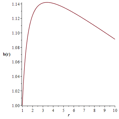
Figure 10: $b(r)$ with $\eta=1.01$, $r_{0}=1$, $B=3$, and $m=2$.

Using Eq. (52) into Eqs. (28)-(30), we get

$$\rho=\frac{-(\eta-1)Br^{(m+1)}+\exp(c-\frac{1}{mBr^{m}})}{Br^{(m+3)}(8\pi_{F}+2\lambda)},$$ (55)

$$p_{r}=\frac{r(\eta-1)-\exp(c-\frac{1}{mBr^{m}})}{r^{3}(8\pi_{F}+2\lambda)},$$ (56)

$$p_{t}=\frac{(Br^{m}-1)\exp(c-\frac{1}{mBr^{m}})}{2Br^{(m+3)}(8\pi_{F}+2\lambda)}.$$ (57)

NEC for this model is given by

$$\rho+p_{r}=\frac{\exp(c-\frac{1}{mBr^{m}})(1-Br^{m})}{Br^{(m+3)}(8\pi_{F}+2\lambda)},$$ (58)

$$\rho+p_{t}=\frac{-2(\eta-1)Br^{(m+1)}+\exp(c-\frac{1}{mBr^{m}})(Br^{m}+1)}{2(Br^{(m+3)})(8\pi_{F}+2\lambda)}.$$ (59)

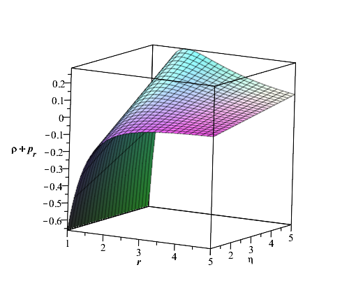
Figure 11: Validity region of NEC, $\rho+p_{r}\leq 0$, with $r_{0}=1$, $B=4$, $m=3$, and $\lambda=-12$.

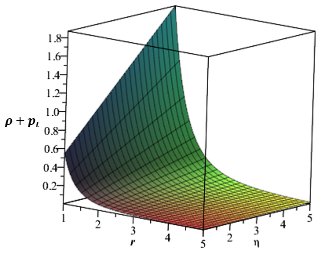
Figure 12: Validity region of NEC, $\rho+p_{t}\geq 0$, with $r_{0}=1$, $B=4$, $m=3$, and $\lambda=-12$.

DEC for this model is given by

$$\rho-p_{r}=\frac{-2(\eta-1)(Br^{(m+1)}+1)+\exp(c-\frac{1}{mBr^{m}})(1+Br^{m})}{Br^{(m+3)}(8\pi_{F}+2\lambda)},$$ (60)

$$\rho-p_{t}=\frac{-2(\eta-1)Br^{(m+1)}+\exp(c-\frac{1}{mBr^{m}})(3-Br^{m})}{2(Br^{(m+3)})(8\pi_{F}+2\lambda)}.$$ (61)

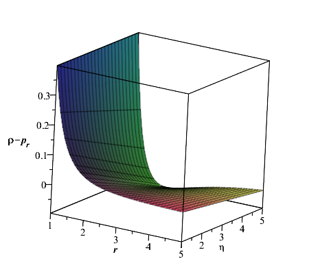
Figure 13: Validity region of DEC, $\rho\geq\lvert p_{r}\lvert$, with $r_{0}=1$, $B=4$, $m=3$, and $\lambda=-11$.

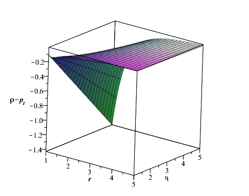
Figure 14: Validity region of DEC, $\rho\geq\lvert p_{t}\lvert$, with $r_{0}=1$, $B=4$, $m=3$, and $\lambda=-12$.

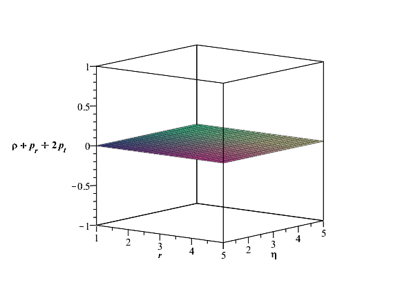
Figure 15: The SEC term: $\rho+p_{r}+2p_{t}=(\rho+p_{r}+2p_{t})(r,n)$ with $r_{0}=1$.

5 Discussions and Results

In the present theory, we have studied the SWH models with the $f(R,T)$ gravitation theories in the context of Finsler geometry using polynomial shape function and discovered a few interesting characteristics. Here, we mainly focused on the case $f(R,T)=R+2f(T)$, where $f(T)=\lambda{T}$ and $\lambda$ is a constant parameter. The uncertainty of $f(R,T)$ gravity WHs will depend on the range of choice of parameter. Regarding this, many researchers have been working on $f(R,T)$ MGT. Among them, H. M. Manjunatha et al. [38] (2022) investigated the models of WH in $f(R)$ gravity with the Finslerian approach using the exponential shape function by taking $\lambda=0$. In Ref. Manjunath Malligawad et al. [45] (2023), authors discussed the WH model using an exponential shape function in the perspective of Finsler geometry with $f(R,T)$ MGT by taking $\lambda=12.5$.
In the previous section, we plotted the embedded 2-D graph for Finslerian WH Fig. (2). Now we will analyze our results by comparing them with the work done by Manjunath Malligawad.

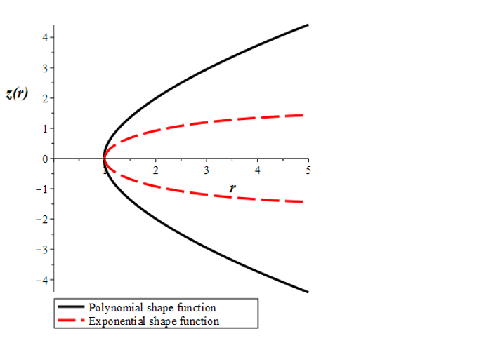
Figure 16: Comparison of polynomial and exponential shape functions with $r_{0}=1$.

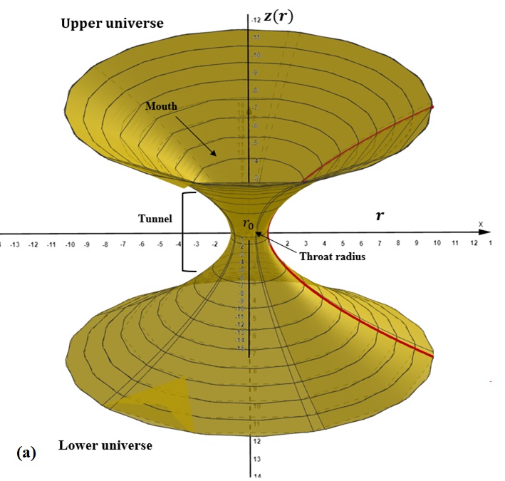
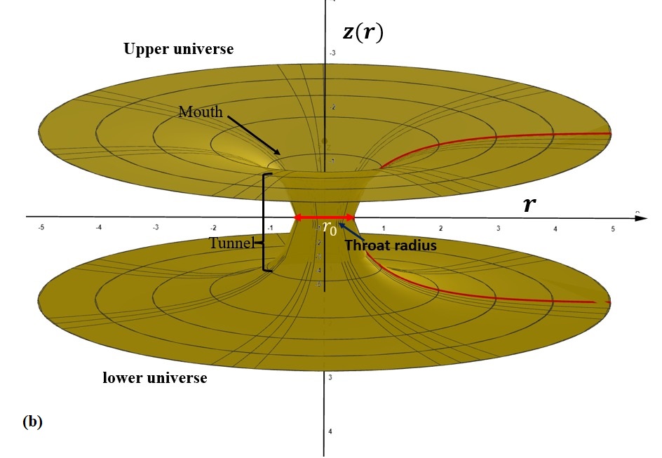
Figure 17: (a) Embedded 3-D WH plot for the Polynomial shape function. (b) Embedded 3-D WH plot for the Exponential shape function.

In the Fig. (16), one can spot the difference in the shape of the two various kinds of shape function $b(r)=r_{0}e^{1-\frac{r}{r_{0}}}$ and $b(r)=(1-\eta)r+Ar^{1+2n}$ respectively with throat value $r_{0}=1$ for both functions. We can see the bending of the exponential curve earlier than the polynomial shape function means the flatness of the wormhole for the exponential shape function appears to be larger with a wide range of radius compared to that of the polynomial shape function.

6 Conclusion

In the current article, we have constructed various models of SWHs that match with the $f(R,T)$ theory of gravitation within the Finslerian approach. We will talk about our conclusions regarding the material and geometrical content of those in this part.

By the GR theory, WHs are stuffed with the matter, which is completely different from ordinary matter and is known to be an exotic matter and has a negative mass. Many researchers have found exotic matter to be very useful in studying the violation of various modified theories of gravity accounts for the violation of energy conditions through the effective energy-momentum tensor.

As we discussed in the previous sections, the flaring condition $b^{\prime}(r_{0})<1$, which is necessary to illustrate a WH solution, is obeyed in all the models that we have constructed. For Model 1, $b^{\prime}(r_{0})=-(\eta-1)+1+2n$, which is less than one, since $n$ is negative, corresponding to Eqs. (32)-(33). For Case I of Model 2, $b^{\prime}(r_{0})=-(\eta-1)+\frac{1}{\omega}<1$, since $\omega>1$ and for Case II, $b^{\prime}(r_{0})<1$ implies in $r_{0}>(\frac{1}{B})^{(\frac{1}{m})}$.

Furthermore, the redshift function has been assumed to be constant ($B(r)$ = constant), which means that the hypothetical traveler’s experience of tidal gravitational force is negligible.
Considering the famous paper by M. S. Morris and K. S. Thorne [14], the authors have discovered that in an SWH, $\rho\sim r^{-2}$. We can observe that the proportionality for $r$ when $\omega\rightarrow 1$ is predicted by our solution for $\rho$ in Case I of Model 2 with the same precision. In this instance, however, our results for $\rho$ are consistent with that for Morris-Thorne WHs with a cosmological constant [46] and WHs minimally violating NEC [47].

And we discussed NEC and DEC in Figs. (5)-(8) and Figs. (11)-(14), The study of the traversable WH’s geometry has revealed that the NEC is violated at the WH throat. Thus, NEC’s violation may confirm the existence of exotic matter at the WH throat, which is the fundamental requirement for the existence of traversable WH. In the present models, at the throat of the WH, the weaker inequality $\rho(r_{0})+p_{r}(r_{0})\leq 0$ holds, which intimates that NEC is violated. The authors in [48] derived the validity of NEC, $\rho+p_{r}\geq 0$, by assuming the negative energy density. On the flip side, we have plotted the graph for SEC in Fig. (5) and Fig. (9) and is satisfied in both cases of Model 2, i.e., $\rho+p_{r}+2p_{t}=0$, as one can check Eqs. (28)-(30). This violation provides strong evidence for the presence e of exotic matter at the WH throat and in the sense WHs.

Finally, we would like to add that we adopted a direct and accurate construction for our computations. We have achieved a detailed set of analytical solutions, and the 3-D embedded visualization of the WH plot for the shape function Eq. (13) can conclude that our polynomial Finslerain $f(R,T)$ gravity WH model is physically valid. A similar method can be incorporated in the same scenarios for different alternative gravity theories.

7 Appendix

We have constructed embedded 2-D and 3-D diagrams for the shape function Eq. (32) for better visualization of the WH. We used an equatorial plane $\theta=\frac{\pi}{2}$ at a fixed time or $t$ = constant, and $\eta=1$, from these conditions Eq. (13) reduce into the form

$$F^{2}=-\left(1-\frac{b(r)}{r}\right)^{-1}dr^{2}-r^{2}d\phi{{}^{2}},$$ (62)

the above equation can be written in cylindrical co-ordinates as

$$F^{2}=-dz^{2}-dr^{2}-r^{2}d\phi{{}^{2}}.$$ (63)

$z=z(r)$ represents the embedded surface in 3-dim Euclidean space, we can rewrite Eq. (63) as

$$F^{2}=-\left(1+\left(\frac{dz}{dr}\right)^{2}\right)dr^{2}-r^{2}d\phi^{2}.$$ (64)

Now comparing Eq. (62) and Eq. (64) we have

$$\frac{dz}{dr}=\pm\sqrt{\left(1-\frac{b(r)}{r}\right)^{-1}-1}.$$ (65)

Using Eq. (65) we plotted embedded surface of the WH.

References

- [1] Einstein, A., Rosen, N.: The particle problem in the general theory of relativity. Phys. Rev. D 48, 73 (1935)
- [2] Flamm, L.: Black Holes and Wormholes-The Physics of the Universe. Phys. Z. 17, 448 (1916)
- [3] Misner, C.W., Wheeler, J.A.: Classical physics as geometry. Ann. Phys. (N.Y.) 2, 525 (1957)
- [4] Bhawal, B., Kar, S.: Lorentzian wormholes in Einstein-Gauss-Bonnet theory. Phys. Rev. D 46, 2464 (1992)
- [5] Maeda, H., Nozawa, M.: Static and symmetric wormholes respecting energy conditions in EinsteinGauss-Bonnet gravity. Phys. Rev. D 78, 024005 (2008)
- [6] Abbott, B.P. et al.: Observation of Gravitational Waves from a Binary Black Hole Merger. Phys. Rev. Lett. 116, 061102 (2016)
- [7] Akiyama, K. et al.: Event horizon telescope. Astrophys. J. 875, (2019) L1
- [8] Khatsymovsky, V.: Can wormholes exist? Phys. Lett. B 320, 234 (1994)
- [9] Rahaman, F., Kuhfittig, P.K.F., Saibal, R., Nasarul Islam: Possible existence of wormholes in the galactic halo region. Eur. Phys. J. C 74, 2750 (2014)
- [10] Övgün, A., Halilsoy, M.: Studies on Thin-shells and Thin-shell Wormholes. Astrophys. Space Sci. 361, 214 (2016)
- [11] Margarita Safonova, Torres, F., Romero, E.: Microlensing by natural wormholes: Theory and simulations. Phys. Rev. D 65, 023001 (2001)
- [12] Javed, W. et al.: Weak deflection angle by Casimir wormhole using Gauss-bonnet theorem and its shadow. Phys. Rev. D 99, 084012 (2019)
- [13] Moraes, P.H.R.S., Correaa, R.A.C., Lobatoa, R.V.: Analytical general solutions for static wormholes in gravity. J. Cosmol. Astropart. Phys. 1, (2017)
- [14] Morris, M.S., Thorne, K.S.: Wormholes in spacetime and their use for interstellar travel: A tool for teaching general relativity. Am. J. Phys. 56, 395 (1988).
- [15] Jusufi, K. et al.: Traversable wormholes supported by GUP corrected Casimir energy. Eur. Phys. J. C 80, 127 (2020)
- [16] Richarte, M.G. et al.: Relativistic Bose-Einstein condensates thin-shell wormholes. Phys. Rev. D 96, 084022 (2017)
- [17] Halilsoy, M. et al.: Thin-shell wormholes from the regular Hayward black hole. Eur. Phys. C 74, 2796 (2014)
- [18] Bhatti, M.Z., Yousaf, Z., Ilyas, M.: Existence of wormhole solutions and energy conditions in gravity. J. Astrophys. Astr. 04, 019 (2009)
- [19] Harko, T., Lobo, F.S.N., Nojiri, S. Odintsov, S.D.: gravity. Phys. Rev. D 84, 024020 (2011)
- [20] Momeni, D., Moraes, P.H.R.S., Myrzakulov, R.: Generalized second law of thermodynamics in theory of gravity. Astrophys. Space Sci. 361, 228 (2016)
- [21] Sharif, M., Zubair, M.: Thermodynamics in theory of gravity. JCAP 03, 028 (2012)
- [22] Shamir, M.F.: Locally rotationally symmetric Bianchi type I cosmology in gravity. Eur. Phys. J. C 75, 354 (2015)
- [23] Noureen, I., Zubair, M., Bhatti, A.A., Abbas, G.: Shear-free condition and dynamical instability in gravity. Eur. Phys. J. C 75, 323 (2015)
- [24] Azizi, T.: Wormhole geometries in gravity. Int. J. Theor. Phys. 52, 3486 (2013)
- [25] Zubair, M., Waheed, S., Ahmad, Y.: Static spherically symmetric wormholes in gravity. Eur. Phys. J. C 76, 444 (2016)
- [26] Kuhfittig, P.K.F.: Gravitational lensing of wormholes in the galactic halo region. Eur. Phys. J. C 74, 2818 (2014)
- [27] Bambi, C.: Broad iron line from accretion disks around traversable wormholes. Phys. Rev. D 87, 084039 (2013)
- [28] Harko, T., Kovacs, Z., Lobo, F.S.N.: Electromagnetic signatures of thin accretion disks in wormhole geometries. Phys. Rev. D 78, 084005 (2008)
- [29] Li, Z., Bambi, C.: Distinguishing black holes and wormholes with orbiting hot spots. Phys. Rev. D 90, 024071 (2014)
- [30] Tsukamoto, N., Harada, T. Yajima, K.: Can we distinguish between black holes and wormholes by their Einstein ring systems? Phys. Rev. D 86, 104062 (2012)
- [31] Konoplya, R.A., Zhidenko, A.: Wormholes versus black holes: quasinormal ringing at early and late times. JCAP 12, 043 (2016)
- [32] Nekouee, Z., Narasimhamurthy, S.K., Manjunatha, H.M., Srivastava, S.K.: Finsler–Randers model for anisotropic constant-roll inflation. Eur. Phys. J. Plus 137, 1388 (2022)
- [33] C. Pfeifer, “The Finsler spacetime framework: backgrounds for physics beyond metric geometry”, DESY-THESIS-2013-049.
- [34] Lämmerzahl, C., Lorek, D., Dittus, H.: Confronting Finsler space–time with experiment. Gen. Relativ. Gravit. 41, 1345–1353 (2009)
- [35] Bubuianu, L., Vacaru, S.I.: Axiomatic formulations of modified gravity theories with nonlinear dispersion relations and Finsler–Lagrange–Hamilton geometry. Eur. Phys. J. C 78, 969 (2018)
- [36] Vacaru, S.I.: Principles of Einstein–Finsler gravity and perspectives in modern cosmology. Int. J. Mod. Phy. D 21, 1250072 (2012)
- [37] Chang, Z., Li, X.: Modified Newton’s gravity in Finsler Space as a possible alternative to dark matter hypothesis. Phys. lett. B 668, 453-456 (2008)
- [38] Manjunatha, H.M., Narasimhamurthy, S.K.: The wormhole model with an exponential shape function in the Finslerian framework. Chin. J. Phys. 77, 1561–1578 (2022)
- [39] Li, X., Chang, Z.: Exact solution of vacuum field equation in Finsler spacetime. Phys. Rev. D 90, 064049 (2014)
- [40] Cataldo, M., Meza, P., Minning, P.: - dimensional static and evolving Lorentzian wormholes with a cosmological constant. Phys. Rev. D 83, 044050 (2011)
- [41] Rahaman, F. et al.: Wormhole with varying cosmological constant. Gen. Rel. Grav. 39, 145 (2007)
- [42] Garcia, N.M., Lobo, F.S.N.: Wormhole geometries supported by a nonminimal curvature-matter coupling. Phys. Rev. D 82, 104018 (2010)
- [43] Hochberg, D., Visser, M.: Null Energy Condition in Dynamic Wormholes. Phys. Rev. Lett. 81, 786 (1998)
- [44] Rahaman, F. et al.: Conical Thin Shell Wormhole from Global Monopole: A Theoretical Construction. Acta Phys. Polon. B 40, 25 (2009)
- [45] Manjunath Malligawad, Narasimhamurthy, S.K., Nekouee, Z., Mallikarjun, Y.: The Finslerian Wormhole model with gravity. arXiv:2302.02983 [gr-qc] (Communicated)
- [46] Lemos, J.P.S. et al.: Morris-Thorne wormholes with a cosmological constant. Phys. Rev. D 68, 064004 (2003)
- [47] Bouhmadi-Lopez, M. et al.: Wormholes minimally violating the null energy condition. JCAP 11, 007 (2014)
- [48] Nandi, K.K., Bhattacharjee, B., Alam, S.M.K., Evans, J.: Brans- Dicke wormholes in tha Jordan and Einstein frames. Phys. Rev. D 57, 823 (1998)