HOPE: Human-Centric Off-Policy Evaluation for
E-Learning and Healthcare

Abstract.

Reinforcement learning (RL) has been extensively researched for enhancing human-environment interactions in various human-centric tasks, including e-learning and health care. Since deploying and evaluating policies online are high-stakes in such tasks, off-policy evaluation (OPE) is crucial for inducing effective policies. In human-centric environments, however, OPE is challenging because the underlying state is often unobservable, while only aggregate rewards can be observed (students’ test scores or whether a patient is released from the hospital eventually). In this work, we propose a human-centric OPE (HOPE) to handle partial observability and aggregated rewards in such environments. Specifically, we reconstruct immediate rewards from the aggregated rewards considering partial observability to estimate expected total returns. We provide a theoretical bound for the proposed method, and we have conducted extensive experiments in real-world human-centric tasks, including sepsis treatments and an intelligent tutoring system. Our approach reliably predicts the returns of different policies and outperforms state-of-the-art benchmarks using both standard validation methods and human-centric significance tests.

1. Introduction

Off-policy evaluation (OPE) sits at the epicenter of offline Reinforcement Learning (RL) research Doroudi et al. (2017); Nachum et al. (2019); Jiang and Li (2016); Thomas and Brunskill (2016), which estimates the performance of an RL-induced policy leveraging prior knowledge obtained from historical data. OPE is especially important in human-centric environments where the execution of a bad policy can be costly and dangerous. For example, in healthcare, an overestimated policy could be ineffective and even increase mortality by wrong treatments. There are at least two main challenges for OPE to work with human-centric environments. One is that the underlying state of a human-centric environment is usually unobservable Mandel et al. (2014); Cassandra (1998), resulting in a partially observable Markov decision process (POMDP). Specifically, the observations may not contain sufficient information to fully reconstruct the underlying states. For example, the population considered in the environment could change over time, and their characteristics may be varied across different cohorts. In e-learning, student backgrounds can vary from semester to semester; similarly, in healthcare, patient demographics can change in hospitals across different regions Payne et al. (2017); Khoshnevisan and Chi (2021). The other challenge is that only an aggregated (or delayed) reward can be observed after a certain period of time, where all immediate rewards in between are often missing. The most appropriate rewards in e-learning and healthcare are student learning performance and patient outcomes, which are typically unavailable until the entire trajectory is complete. This is due to the complex natures of both learning and disease progression, which make it difficult to assess students’ learning or patient health states moment by moment. More importantly, many instructional or medical interventions that boost short-term performance may not be effective over the long term. Different from delayed rewards in classic mouse-in-the-maze situations where agents receive insignificant rewards along the path and a significant reward in the final goal state (the food), in e-learning and healthcare, there are immediate rewards along the way but they are often unobservable.

Prior OPE work Nachum et al. (2019); Jiang and Li (2016); Abe and Kaneko (2021); Gao et al. (2023) have achieved outstanding performance in simulated environments such as Mujoco Todorov et al. (2012). However, one may not be able to directly apply such methods toward human-centric environments, since immediate rewards are missing and the environment is partially observable. A possible way is assuming the rewards are sparse that only indicate whether a task is completed partially or fully. Sparse rewards typically correspond to the attainment of some particular tasks such as a robot attaining designated waypoints which provide little feedback for immediate steps Rengarajan et al. (2022). In many human-centric tasks, interaction outcomes can be gradually improved step-by-step and the immediate reward on each step can be meaningful by itself. For example, students’ cognitive outcomes and learning performance are gradually improved during interaction with the intelligent tutor in college Marwan et al. (2020). It has been found that immediate rewards are more effective than sparse rewards, toward evaluating decision outcomes Azizsoltani and Jin (2019). Moreover, in human-centric environments, policy performance may be correlated with the horizon of the environment. For example, medical interventions that have shown good short-term performance may not be effective over the long-term Azizsoltani and Jin (2019). Consequently, it is important to reconstruct immediate rewards for OPE to work effectively in human-centric environments.

On the other hand, prior evaluation metrics for OPE are generally error metrics (e.g., absolute error, rank correlations) proposed by Fu et al. (2021); Voloshin et al. (2019), while human-centric research often emphasizes the need for statistical significance test in empirical study Guilford (1950); Zhou et al. (2022). For example, rank correlation summarizes the performance of a set of policies’ relative rankings using averaged returns. Statistical significance tests can tell how likely the relationship we have found is due only to random chance across samples, and they are commonly employed and easier to be interpreted by domain experts Guilford (1950); Ju et al. (2019). The framework for validating OPE in human-centric environments may need to be extended beyond error metrics.

In this work, we propose a human-centric OPE (HOPE) approach to tackle the two challenges above. Specifically, it first reconstructs immediate rewards from the aggregated rewards. Then, importance sampling is used to process the reconstructed rewards and estimate expected total returns. Any existing OPE method can be used jointly with the reconstructed rewards to estimate expected returns. We validate HOPE on two typical real-world human-centric tasks in healthcare and e-learning, i.e. sepsis treatments and an intelligent tutoring system (ITS), and extend existing validation frameworks with significance tests for human-centric environments. To summarize, our work has at least three main contributions:

$\bullet$ To the best of our knowledge, HOPE is the first OPE approach that tackles both partial observability and aggregated rewards. We also provide theoretical bound for HOPE.

$\bullet$ HOPE is extensively validated through real-world environments in real-world human-centric environments including e-learning and healthcare. The results show that our approach outperforms the state-of-the-art OPE approaches.

$\bullet$ We introduce significance tests on top of existing OPE validation frameworks, to facilitate comprehensive study and comparison of OPE methods in human-centric environments.

2. Related Work

In e-learning and healthcare, RL has been widely investigated to learn policies from historical user interaction data Nie et al. (2022); Gao et al. (2022d). However, deploying and evaluating policies online are high stakes in such domains, as a poor policy can be fatal to humans in healthcare. It’s thus crucial to propose effective OPE methods for human-centric environments. OPE is used to evaluate the performance of a target policy given historical data drawn from (alternative) behavior policies. Classic methods, such as expected cumulative reward (ECR) Tetreault and Litman (2006), have been employed in real-world applications such as e-learning Chi et al. (2011). However, ECR is not statistically consistent, which is a significant concern for high-stakes domains Mandel et al. (2014). In practice, researchers have found that selected policies based on ECR were even not effective compared to random policies with real students in terms of human-centric significant test Chi et al. (2011); Shen and Chi (2016).

Various contemporary OPE methods have been proposed and can be divided into three general categories Voloshin et al. (2019): 1) Inverse Propensity Scoring (IPS) Precup (2000); Doroudi et al. (2017); 2) Direct Methods Jiang and Li (2016); Paduraru (2013); Le et al. (2019); Harutyunyan et al. (2016); Munos et al. (2016); Farajtabar et al. (2018); Liu et al. (2018); Nachum et al. (2019); Uehara et al. (2020); Xie et al. (2019); Yang et al. (2022); 3) Hybrid Methods Jiang and Li (2016); Thomas and Brunskill (2016). IPS has been widely investigated in statistics Powell and Swann (1966); Horvitz and Thompson (1952) and RL Precup (2000), with the key idea to reweigh the rewards in historical data using the importance ratio between $\beta$ and $\pi$. IPS yields consistent estimates and it has several variations including IS Precup (2000), WIS Precup (2000), PDIS Precup (2000), and PHWIS Doroudi et al. (2017), etc. Direct Methods directly estimate the value functions of the evaluation policy. For example, FQE Le et al. (2019) is functionally a policy evaluation counterpart to batch Q-learning. DualDICE Nachum et al. (2019) estimates the discounted stationary distribution ratios, which measure the likelihood that $\pi$ will experience the state-action pair normalized by the probability with which the state-action pair appears in the off-policy data. Hybrid Methods combine aspects of both IPS and direct methods. For example, DR Jiang and Li (2016) is an unbiased estimator leveraging a direct method to decrease the variance of the unbiased estimates produced by IS. These OPEs have achieved desirable performance in simulated environments. Recently, a few approaches have proposed OPE targeting some real-world tasks such as robotic grasping Irpan et al. (2019); Nie et al. (2021); Chandak et al. (2021); Gao et al. (2022c). The proposed methods generally assume the rewards are observable from the environment or sparse. It lacks investigation into the effectiveness of applying the existing OPE methods in real-world human-centric environments.

Recently, researchers have recognized the partial observability of human-centric environment and proposed OPE for POMDPs Tennenholtz et al. (2020); Bennett et al. (2021); Shi et al. (2022); Uehara et al. (2022). They assume that the underlying states may not exist and treat them as confounding for policy evaluation. For example, Tennenholtz et al. propose a method for POMDP with unobserved confounding and compare their method to IS in carefully-designed synthetic environments Tennenholtz et al. (2020). The results show that their proposed method can outperform IS under certain levels of confounding. In practice, such as in our intelligent tutoring experiment with real students, confounding is agnostic and unable to control, accompanied by missing immediate rewards. Our goal is to utilize limited observable information from real-world e-learning and healthcare environments, and effectively estimate policy performance with both partial observability and missing immediate rewards.

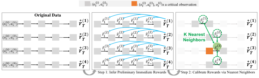
Figure 1. Illustration of reconstructing immediate rewards. First, the preliminary rewards are inferred from aggregated rewards. Then, the immediate rewards on critical observations are calibrated by averaging from nearest neighbors.

3. Human-Centric OPE (HOPE)

Problem Definition: We consider the human-centric environment as a partially observable Markov decision process (POMDP), which is a tuple $(\mathcal{S,A,O},\mathcal{P},\Omega,R,\gamma)$. The state space $\mathcal{S}$ is assumed unknown. Moreover, $\mathcal{A}$ represents the action space, $O$ is the observation space, and $\mathcal{P}$ defines transition dynamics from the current state to the next states given an action. The observation model $p(o|s)\sim\Omega$ is also assumed unknown. $R$ is the immediate reward function, and $r_{t}=R(s_{t},a_{t})$ are the immediate rewards. $\gamma\in(0,1]$ is discount factor. Each episode has a finite horizon $T$. In general, at time-step $t$, the agent is given an observation $o_{t}\in\mathcal{O}$ by the environment, then chooses an action $a_{t}\in\mathcal{A}$ following some policy $\pi:\mathcal{O}\rightarrow\mathcal{A}$. Then, the environment provides the immediate reward $r_{t}$ and next observation $o_{t+1}$. In human-centric tasks, it is common that the immediate rewards $r_{t}$ are unknown for most $t\in[1,T]$ in a trajectory. However, we assume that an aggregated reward $\mathring{r}_{t}=\sum_{i=t-W}^{t}\gamma^{i-t+W+1}r_{i}$ is issued by the environment every $W$ steps, quantifying the summed immediate rewards obtained between $(t-W)$-th and $t$-th steps.

Off-Policy Evaluation in POMDP: the goal of OPE under POMDP is to estimate the expected total return over the target policy $\pi$, $V^{\pi}=\mathbb{E}[\sum_{t=1}^{T}{\gamma^{t-1}r_{t}}|a_{t}\sim\pi]$, using historical data collected over a behavioral policy $\beta\neq\pi$ deployed to the environment. Specifically, the historical data $\mathcal{D}=\{...,[...,(o_{t},a_{t},r_{t},o^{\prime}_{t}),...]^{(i)},...\}^{N}_{i=1}$ consist of a set of $N$ trajectories, where each trajectory is denoted as $\tau^{(i)}$.

Figure 1 illustrates how HOPE addresses the two major challenges of OPE in human-centric environments: partial observability and aggregated rewards. Specifically, it first infers preliminary immediate rewards from aggregated rewards (Step 1) , and reconstructs immediate rewards $r_{t}$ using nearest neighbors from trajectories $\mathcal{D}$ (Step 2), which takes into account the uncertainty introduced by partial observability. The intuition of Step 2 follows findings presented in previous research Yang et al. (2020); Keramati et al. (2022); Gao et al. (2021), where humans with similar underlying states can present similar behaviors. Then, we use a general method, weighted importance sampling, to process the reconstructed rewards and estimate the expected total return $V^{\pi}$, since it is the most straightforward approach and can help isolate the source of improvements brought in by the immediate rewards reconstruction framework we propose.

3.1. Reconstruct Immediate Rewards via Nearest Neighbors

In human-centric environments, immediate rewards are generally not available, while the aggregated rewards themselves may not provide full information that can be directly used to estimate the expected total return of a target policy. Although prior works has noted that estimating immediate rewards can provide useful information toward training RL policies Mataric (1994); Azizsoltani and Jin (2019), it has not be extensively investigated in the context of OPE; since prior OPE works generally assume immediate rewards are observable from the environment or sparse. In many human-centric tasks, interaction outcomes can be gradually improved step-by-step and each immediate reward on each step can represent meaningful information by itself. Therefore, we propose to reconstruct immediate rewards from historical data, aiming to enrich the information provided for OPE.

In the OPE problem we consider, the underlying state is unobservable due to POMDP. And the aggregated rewards are assumed to be obtained at the end of an episode following $\mathring{r}=\sum_{t=1}^{T}{\gamma^{t}r_{t}}$, with $T$ being the horizon of the environment. In prior work, function approximation can be used to infer immediate rewards $r_{t}$ from the aggregated rewards $\mathring{r}$ Azizsoltani and Jin (2019). Consequently, we first produce rough per-step preliminarily reconstructed reward $\tilde{r}$ taking as inputs observations and actions, $\tilde{r}=f(o_{t},a_{t}|\theta)$, and trained toward, i.e.,

$$\min_{\theta}l(\theta)=\frac{1}{N}\sum\limits_{i=1}^{N}\big{(}\mathring{r}-\sum_{t=1}^{T}{\gamma^{t-1}\tilde{r}}\big{)}^{2}.$$ (1)

We keep the objective straightforward and use a standard training method in Ausin et al. (2021), so that the source of performance improvements can be isolated. For conciseness, we refer to $\tilde{r}$ as preliminary immediate rewards throughout the rest of the paper. In our experiments described in Section 4.5, we compare it to treating the rewards as sparse, and the results present the effectiveness of the preliminary immediate rewards reconstruction procedure.

Consider that the mapping $f:\mathcal{O}\times\mathcal{A}\rightarrow\mathbb{R}$ learned above may not perfectly reconstruct the immediate reward function $R:\mathcal{S}\times\mathcal{A}\rightarrow\mathbb{R}$, since the observation model $p(o|s)$ and state space $\mathcal{S}$ are both assumed unknown. Previous research have found that humans with similar underlying state can be observed similar behaviors Yang et al. (2020); Yin et al. (2020), and some observations may provide critical information over others Torrey and Taylor (2013). We then follow such intuitions and introduce a remedy that uses $\tilde{r}_{t}$ and its nearest neighbours, from trajectories that are similar to each other, to reconstruct immediate rewards $r_{t}$ more accurately.

Specifically, to capture the information pertaining to the underlying states, we define the reconstructed immediate reward $\hat{r}_{t}$ considering both average rewards associated with neighboring trajectories and observations that may provide more critical information over others, by which we call critical observations, i.e.,

$$\hat{r}_{t}=\mathbbm{1}(o_{t}\in O^{*})\bar{r}_{t}+\mathbbm{1}(o_{t}\notin O^{*})\tilde{r}_{t},$$ (2)

where $O^{*}$ is the set of critical observations, $\mathbbm{1}(\cdot)$ is an indicator function.

We first introduce how to identify the critical observations. Given that $Q$-functions, $Q^{\pi}(o,a)$, representing the expected return of taking action $a$ at observation $o$, the difference of $Q^{\pi}$ between any two actions (over the same $o$) can be used to quantify the magnitude of the difference in the final outcomes. As a result, we choose to leverage such $Q$-difference toward determining critical observations for OPE. A formal definition of a critical observation can be found below.

Definition 0 (Critical Observation).

In a discrete action POMDP, observation $o$ is a critical observation if there exists a constant $h$ such that the maximum difference of $Q^{\pi}(o,a),a\in\mathcal{A}$ is greater than $h$, i.e.,

$$\max_{a^{\prime},a^{\prime\prime}\in\mathcal{A}}(Q^{\pi}(o,a^{\prime})-Q^{\pi}(o,a^{\prime\prime}))>h.$$ (3)

In Fig. 2, we illustrate how critical observations are identified using the threshold $h$. The need of critical observations is further justified by ablation study in Section 4.5.

Denote $\hat{r}^{(i)}_{t}$ as the reconstructed immediate reward at time-step $t$ on trajectory $\tau^{(i)}$. We define the averaged reward $\bar{r}^{(i)}_{t}$ associated with critical observation $o^{(i)}_{t}$ as an average of preliminary immediate rewards $\tilde{r}$ that occur at neighboring events following

$$\bar{r}^{(i)}_{t}=\frac{1}{K}\sum_{k}{\tilde{r}^{(k)}_{t^{\prime}}},$$ (4)

where the summation is performed over all $\mathring{r}^{(k)}_{t^{\prime}}$ and $K$ is the total number of nearest neighbours pertaining to the algorithm 1. Specifically, we define that two trajectories are neighbors if they have similar visitation distributions over the observation and action spaces, following

$$d(\tau^{(i)},\tau^{(k)})=similarity(o^{(i)},o^{(k)})+similarity(a^{(i)},a^{(k)})$$ (5)

where the similarity of distributions can be calculated by some measures such as Kullback-Leibler (KL) divergence Kullback and Leibler (1951). Then we define that two observations are neighbors if they are from two neighboring trajectories, and share the most similar observations, since the moment that sharing similar observations from the similar trajectories may represent close underlying state of humans Yang et al. (2020); Yin et al. (2020). To calculate similarity between two observations, one can use distance measures such as Euclidean. We can always find one and only one neighboring observation on a given neighboring trajectory, by breaking ties appropriately – such as selecting the earliest observation. Algorithm 1 summarizes how to find the K-nearest neighbors of $o_{t}^{(i)}$. In our experiment, the proposed distance to find nearest neighbors is compared to random selection in Section 4.5, and the results show the superior performance of the proposed distance.

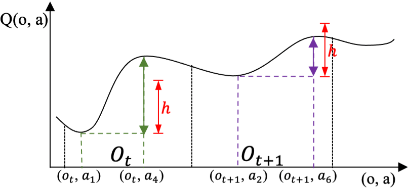
Figure 2. Identify critical observations based on the maximum difference of $Q$ values. $o_{t}$ is a critical observation with difference of $Q$ greater than a threshold $h$.

0:  Historical data $\mathcal{D}$, hyper-parameter $K$.

0:  

1:  Initialize an empty set $Z^{i}_{t}$.

2:  for each trajectory $\tau^{(j)}\in\mathcal{D}$ do

3:     Calculate the distance $d(\tau^{(i)},\tau^{(j)})$ following (5).

4:  end for

5:  Arrange $d(\tau^{(i)},\tau^{(j)}),j\in N$ in non-decreasing order, take the first $K$ elements and find the corresponding trajectories as neighboring trajectories of $\tau^{(i)}$.

6:  for each neighboring trajectory $\tau^{(k)}$ of $\tau^{(i)}$ do

7:     for each observation $o^{(k)}_{t^{\prime}}\in\tau^{(k)}$ do

8:        Calculate the distance $l^{ik}_{tt^{\prime}}$ between $o^{(k)}_{t^{\prime}}$ and $o^{(i)}_{t}$.

9:     end for

10:     Arrange $l^{ik}_{tt^{\prime}},t^{\prime}\in T$ in non-decreasing order, take the first element and find the corresponding observation $o^{(k)}_{t^{\prime}}$ as neighboring observation of $o^{(i)}_{t}$.

11:     $Z^{i}_{t}\leftarrow Z^{i}_{t}\cup o^{(k)}_{t^{\prime}}$

12:  end for

13:  Return the set $Z^{i}_{t}$.

Algorithm 1 Find K Nearest Neighbors of $o^{(i)}_{t}$.

3.2. HOPE

Based on the proposed solutions regarding the challenges within human-centric environment, we propose our human-centric OPE (HOPE) by incorporating estimated immediate rewards with weighted importance sampling (WIS). Let $w_{i}:=\Pi_{t=1}^{T}{\pi(a^{(i)}_{t}|o^{(i)}_{t})/\beta(a^{(i)}_{t}|o^{(i)}_{t})}$ be an importance weight, which is the probability of the first $T$ steps of $\tau^{(i)}$ under the target policy, $\pi$, divided by its probability under the behavior policy, $\beta$ Precup (2000). The estimated return of HOPE for an target policy $\pi$ is

$$V^{\pi}(\mbox{HOPE})=\frac{1}{\sum_{i=1}^{N}{w_{i}}}\sum_{i=1}^{N}{w_{i}}\sum_{t=1}^{T}{\gamma^{t-1}\hat{r}^{(i)}_{t}},$$ (6)

We choose to use WIS here since it is the most straightforward approach. Moreover, this can help isolate the source of improvements brought in by immediate rewards reconstruction framework we propose. Prior work note that the lower variance of WIS may produce a larger reduction in expected square error than the additional error incurred due to the bias compared to some unbiased OPE such as importance sampling (IS) in practice Thomas et al. (2015). Our real-world experimental results in Section 4 further support this.

In general, the importance weight assumes that the support of the evaluation policy $\pi$ is a subset of the behavior policy $\beta$, which is enforced by Assumption 1 Thomas (2015):

Assumption 1.

If $\pi(a|o)\neq 0$, then $\beta(a|o)\neq 0$, where $a\in\mathcal{A},o\in\mathcal{O}$.

Upper and Lower Bounds of HOPE

We define $\delta^{ik}$ as the event where $\tau^{(k)}$ is a neighbor of $\tau^{(i)}$. Also, we define the counts of neighboring events as $K=\sum_{k=1}^{N}\mathbbm{1}(\delta^{ik})$, where $\mathbbm{1}(\cdot)$ is the indicator function. We then construct the nearest-neighbors matrix: $M^{ik}=\frac{\mathbbm{1}(\delta^{ik})}{K}$. As The $N\times N$ matrix $M^{ik}$ can be computed from the data and be used to compute the estimated immediate rewards for all observation-action pairs using the following proposition.

Proposition 0.

For all transitions in the data, the estimated immediate rewards for corresponding observation-action pairs are given by

$$\hat{r}^{(i)}_{t}=\sum_{k}M^{ik}\equiv[\textbf{Mu}]_{i}$$ (7)

Proof.

A given reward on trajectory $i$ at timestamp $t$, that averaging over all rewards on trajectory $j$ at timestamp $t^{\prime}$ such that $\delta_{tt^{\prime}}^{ij}$ holds, can be written as $\frac{1}{K}\sum_{(j,t^{\prime}):\delta_{tt^{\prime}}^{ij}}=\sum_{j,t^{\prime}}\frac{\mathbbm{1}(\delta_{tt^{\prime}}^{ij})}{K}=\sum_{j,t^{\prime}}M_{tt^{\prime}}^{ij}$. Therefore, assume $u(o,a)$ is a function over the observation-action space and u is the vector containing the quantity $u_{i}=u(o^{(i)},a^{(i)})$ for every $(o^{(i)},a^{(i)})$, the nearest-neighbor estimation of $u(o^{(i)},a^{(i)})$ is given by $[\textbf{Mu}]_{i}$. ∎

In the case of $\tilde{r}\in[\tilde{r}_{lb},\tilde{r}_{ub}]$, $\hat{r}\in[\tilde{r}_{lb},\tilde{r}_{ub}]$ according to Proposition 2. Denote the returns of trajectory $\tau^{(i)}$ as $G(\tau^{(i)})$. Following Thomas (2015), we also write $G(\tau^{(i)})\in[0,1]$ s.t. $G(\tau^{(i)}):=\frac{(\sum_{t=1}^{T}\gamma^{t-1}\hat{r}^{(i)}_{t})-G_{lb}}{G_{ub}-G_{lb}}$ to denote quantification of how good a trajectory $\tau^{(i)}$ is. Then the HOPE estimation is written by $\frac{1}{\sum_{n=1}^{N}{w_{i}}}\sum_{i=1}^{N}{w_{i}}G(\tau^{(i)})=\frac{\sum_{i=1}^{N}{w_{i}}G(\tau^{(i)})}{\sum_{i=1}^{N}{w_{i}}}$. Then the upper and lower bound of HOPE estimation can be calculated using the following lemma, the proof of which is given in Thomas (2015).

Lemma 0.

Let $\pi$ and $\beta$ be any policy such that Assumption 1 holds, then for any constant integer $m\geq 1$, $\mathbb{E}[\prod^{m}_{t=1}\frac{\pi(a_{t}|o_{t})}{\beta(a_{t}|o_{t})}|\tau\sim\beta]=1.$

From Lemma 3, with the number of samples increasing, the denominator of HOPE tends towards $n$. HOPE estimator is bounded within $[0,1]$, and so $\rho^{HOPE}_{lb}(\pi,\beta)=0$ and $\rho^{HOPE}_{ub}(\pi,\beta)=1$ for all $\pi$ and $\beta$, where $\rho(\pi)=\mathbb{E}[G(\tau)|\tau\sim\beta]$.

Consistency of HOPE

We also show that HOPE is a consistent estimator of $\rho(\pi)$ if there is a single behavior policy (Theorem 4) or if there are multiple behavior policies that satisfy a technical requirement (Theorem 5), following work by Thomas (2015).

Theorem 4.

If Assumption 1 holds and there is only one behavior policy, then HOPE is a consistent estimator of $\rho(\pi)$.

Proof.

When there is only one behavior policy, HOPE estimation can be rewrote as $\frac{\frac{1}{N}\sum_{i=1}^{N}{w_{i}}G(\tau^{(i)})}{\frac{1}{N}\sum_{i=1}^{N}{w_{i}}}$ by multiplying both its numerator and denominator by $\frac{1}{N}$. Then the numerator is equal to $IS^{\pi}$, which is a consistent estimator of $\rho(\pi)$ as proved in prior work Precup (2000); Thomas (2015)), thus the numerator converges almost surely to $\rho(\pi)$. For the denominator, by Lemma 3, we have that

$$\mathbb{E}[\prod^{T}_{t=1}\frac{\pi(a^{(i)}_{t}|o^{(i)}_{t})}{\beta(a^{(i)}_{t}|o^{(i)}_{t}})]=1,\text{for all }i\in[{1,\dots,N}].$$ (8)

Each term $\prod^{T}_{t=1}\frac{\pi(a^{(i)}_{t}|o^{(i)}_{t})}{\beta(a^{(i)}_{t}|o^{(i)}_{t})}$ is identically distributed for each $i\in{[1,\dots,N]}$, as there is only one behavior policy. By the Khintchine strong law of large numbers Sen and Singer (1994), we have that

$$\frac{1}{N}\sum^{N}_{i=1}\prod^{T}_{t=1}\frac{\pi(a^{(i)}_{t}|o^{(i)}_{t})}{\beta(a^{(i)}_{t}|o^{(i)}_{t})}\xrightarrow{\text{a.s.}}1.$$ (9)

By the property of almost sure convergence Jiang (2010), HOPE converges almost surely to $\rho(\pi)$, and so HOPE is a consistent estimator of $\rho(\pi)$. ∎

We also provide the proof for the consistency of HOPE when there are multiple behavior policies.

Theorem 5.

If Assumption 1 holds and there exists a constant $\epsilon>0$ such that $\beta_{i}(a|o)\geq\epsilon$ for all $i\in\{1,\dots,N\}$ and $(a|o)$ where $\pi(a|o)\neq 0$, then HOPE is a consistent estimator of $\rho(\pi)$ if there are multiple behavior policies.

Proof.

When there are multiple behavior policies, similar to the proof of Theorem 4, the numerator is equal to $IS^{\pi}$. The numerator converges almost surely to $\rho(\pi)$. For the denominator, by Lemma 3 we have that Equation 8 holds. Each term $\prod^{T}_{t=1}\frac{\pi(a^{(i)}_{t})|o^{(i)}_{t}}{\beta_{i}(a^{(i)}_{t})|o^{(i)}_{t}}\in[0,\frac{1}{\epsilon^{T}}]$ and therefore has bounded variance. By the Kolmogorov strong law of large numbers Sen and Singer (1994), we have that almost surely convergence 9 holds. Therefore, HOPE is a consistent estimator of $\rho(\pi)$ if there are multiple behavior policies. ∎

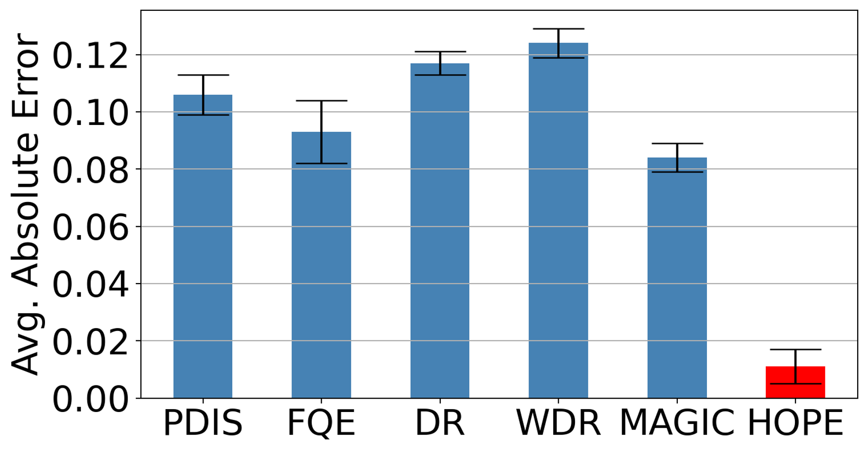
Figure 3. Average absolute error and standard deviation from synthetic sepsis environment ($\gamma$=0.99). IS, WIS, PHWIS, DualDICE are unable to select the best policy.

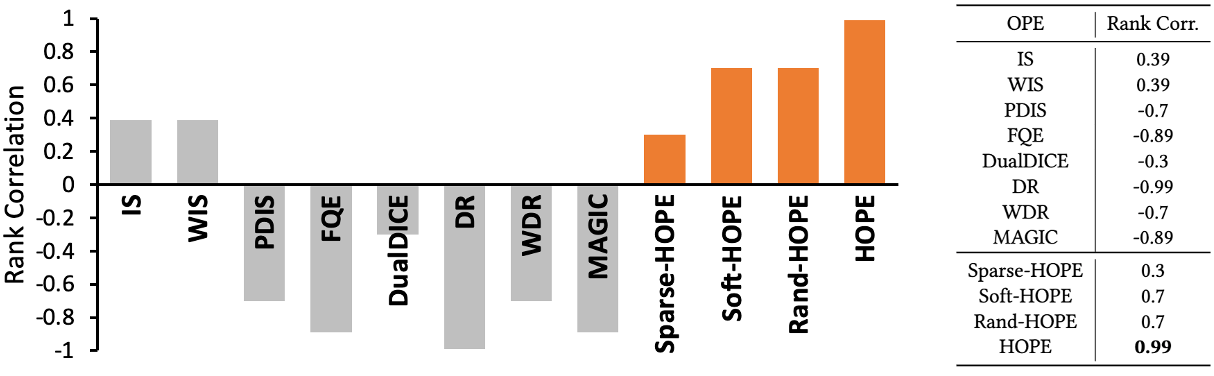
Figure 4. Spearman’s rank correlation coefficient across policies from real-world medical system ($\gamma$=0.99). PHWIS is unable to produce a meaningful result probably due to the highly varied lengths of trajectories.

4. Experiments

We conduct experiments on two real-world human-centric tasks, sepsis treatment, and intelligent tutoring, to validate our proposed approach. Since our focus is the human-centric environments, we don’t conduct experiments on control tasks such as D4RL Fu et al. (2020).

4.1. Benchmarks

We use nine state-of-the-art benchmarks, which cover a variety of approaches that have been explored for OPE: Four IPS methods, including IS Precup (2000), WIS Precup (2000), Per-Decision IS ( PDIS) Precup (2000), and Per-Horizon WIS (PHWIS) Doroudi et al. (2017). For PHWIS, we follow the PHWIS-Behavior as in Doroudi et al. (2017), as we assume the lengths of the trajectories do not depend on the policy that is used to generate them. Two direct methods, Fitted Q Evaluation (FQE) Le et al. (2019) and Dual stationary DIstribution Correction Estimation (DualDICE) Nachum et al. (2019). For FQE, as in Le et al. (2019), we train a neural network to estimate the value of the evaluation policy $\pi_{e}$ by bootstrapping from $Q(o^{\prime},a^{\prime})$. For DualDICE, we use the open-sourced code in its original paper. Three hybrid methods, including Doubly Robust (DR), Weighted DR (WDR) Thomas and Brunskill (2016), and MAGIC Thomas and Brunskill (2016), which finds an optimal linear combination among a set that varies the switch point between WDR and direct methods. For MAGIC, we use the implementation of Voloshin et al. (2019).

4.2. Validating OPE Performance

In this work, we use two types of procedures to validate the performance of OPE methods. We use standard metrics including absolute error, regret@1, and Spearman’s rank correlation coefficient Spearman (1987) that are commonly used in prior OPE approaches. Definitions of these metrics are described in Appendix B. Moreover, we use the human-centric significance test to measure the statistical significance between the OPE-estimated returns across different policies. For each evaluation policy, we use bootstrapping by episodes as introduced in Hao et al. (2021). For e-learning, we also empirically evaluated the induced policies. As for many human-centric tasks, one key measurement for the RL-induced policy is whether they significantly outperform the current expert policy Zhou et al. (2020). Therefore, we conduct a t-test over OPE estimations obtained from bootstrapping. It measures whether there is a significant difference between the mean value of OPE estimations on one policy against another.

4.3. Sepsis Treatment

Sepsis, defined as life-threatening organ dysfunction in response to infection, is the leading cause of mortality and the most expensive condition associated with in-hospital stay, accounting for more than $24 billion in annual costs in the United States Liu et al. (2014). In particular, septic shock, which is the most advanced complication of sepsis due to severe abnormalities of circulation and/or cellular metabolism Bone et al. (1992), reaches a mortality rate as high as 50% Martin et al. (2003). Sepsis treatment is a highly challenging problem and has raised tremendous investigation Gao et al. (2022b, a).

4.3.1. Synthetic Sepsis Environment

We use Oberst and Sontag’s sepsis model Oberst and Sontag (2019) in the management of sepsis in ICU patients. Following the settings from Namkoong et al. (2020), the discrete observation space consists of a binary indicator for diabetes, and four vital signs (heart rate, blood pressure, oxygen concentration, glucose level) that take values in a subset of {very_high, high, normal, low, very_low}. The simulated environment contains a total of 1440 observations, and 8 actions characterized by assigning a binary value (0 or 1) toward each option in {antibiotics, vasopressors, mechanical_ventilation}. The simulation continues either until at most T = 5 (horizon) time steps (0 rewards), death (-1 reward), or discharge (+1 reward). Patients are discharged when all vital signs are in the normal range without treatment. Patients die if at least three vitals are out of the normal range. We use the behavior policy and three evaluation policies following Namkoong et al. (2020). Figure 3 shows that HOPE performs the best in terms of average absolute error across evaluation policies. Detailed results are presented in Appendix B.1.

4.3.2. Real-World Medical System

A medical system is another important domain for OPE, considering the safety of treating patients. In our experiment, we use Electronic Health Records (EHRs) collected from a large hospital in the United States with overall 221,700 visits patients over two years. The observation space consists of 15 continuous sepsis-related clinical attributes, including seven vital signs {HeartRate, RespiratoryRate, PulseOx, SystolicBP, DiastolicBP, MAP, Temperature} and eight lab analytes {Bands, BUN, Lactate, Platelet, Creatinine, BiliRubin, WBC, FIO2}. The size of action space is 4 with two binary treatment options over {antibiotic_administration, oxygen_assistance}. Four stages of sepsis are defined by the clinicians, and the rewards are set for each stage: infection ($\pm$5), inflammation ($\pm$10), organ failure ($\pm$20), and septic shock ($\pm$50). The designated negative rewards are given when a patient enters the corresponding stage and positive rewards are given back when the patient recovers from the stage. The collected trajectories’ lengths range from 1 to 1160. We assume that the clinical care team is well-trained with medical knowledge and follows standard protocols in sepsis treatments, thus we learn the expert policy as introduced in Azizsoltani and Jin (2019). We train policies using Deep Q Network (DQN) Mnih et al. (2015) with varied hyperparameters and select five as evaluation policies as discussed in Appendix B.2. As prior work in sepsis research Komorowski et al. (2018); Azizsoltani and Jin (2019); Raghu et al. (2017) identifies septic shock rate as an important criterion for learning policies, we calculate Spearman’s rank correlation coefficient between the policies’ rank using estimated values given by OPE and the actual policies’ rank in terms of septic shock rates. Experimental details are provided in Appendix B.2.

Figure 4 shows the results of HOPE and benchmarks. The grey-shaded columns represent the benchmark results, and the orange-shaded columns represent the results from HOPE and its variations. Overall, HOPE performs the best in terms of rank correlation. Interestingly, we notice that IS and WIS outperform other benchmarks, while they can be suffering from long-horizon in prior theoretical work Liu et al. (2018). A possible reason is that both methods benefit more from the reduction in expected error than the variance incurred due to horizon under our real-world settings. Similar findings are reported in some long-horizon environments Fu et al. (2021).

Figure 5. Our ITS GUI. The problem statement window (top) presents the statement of the problem. The dialog window (middle right) shows the message the tutor provides to the students. Responses, e.g., writing an equation, are entered in the response window (bottom right). Any variables and equations generated through this process are shown on the variable window (middle left) and equation window (bottom left).

4.4. Real-World Intelligent Tutor

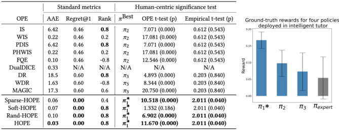
Figure 6. Validating OPE performance (left) and empirical results (right) from real-world intelligent tutoring ($\gamma=0.9$). Left: Standard metrics include average absolute error (AAE), regret@1, and Spearman’s rank correlation coefficient (Rank). The best results on each metric are bolded. Human-centric significance test results include the best policy selected by OPE, offline significance test with bootstrapping on the best policy selected by OPE and expert policy, and empirical significance test on these two policies, at the level of $p<0.05$. The OPE significance test that aligns with the empirical test is bolded. DualDICE estimates the performance of all policies equally, thus its rank-related results are unavailable. Right: Ground-truth rewards for four policies. $\pi_{1}$ receives the highest average reward and is the only policy that differs significantly from $\pi_{expert}$ ($p=0.04$), as indicated by the asterisk.

Intelligent Tutoring Systems (ITSs) are computer systems that mimic aspects of human tutors and have also been shown to be successful VanLehn (2006); Abdelshiheed et al. (2020, 2021). They aim to provide instruction or feedback to support students’ learning, which is an important application of RL to improve students’ engagement and learning outcomes. We use a web-based ITS which teaches computer science students probability knowledge, covering ten major principles such as the complement theorem. Students’ interaction logs are collected over seven semesters of classroom studies (including 1,307 students) in an undergraduate computer science course at a large public university in the United States. Figure 5 shows the GUI of the tutor.

During tutoring, there are many factors that might determine or indicate students’ learning state, but many of them are not well understood by educators. Thus, to be conservative, we extract varieties of attributes that might determine or indicate student learning observations from student-system interaction logs. In sum, 142 attributes with both discrete and continuous values are extracted, which can be categorized into the following five groups:

(i) Autonomy (10 features): the amount of work done by the student, such as the number of times the student restarted a problem;

(ii) Temporal Situation (29 features): the time-related information about the work process, such as average time per step;

(iii) Problem-Solving (35 features): information about the current problem-solving context, such as problem difficulty;

(iv) Performance (57 features): information about the student’s performance during problem-solving, such as percentage of correct entries;

(v) Hints (11 features): information about the student’s hint usage, such as the total number of hints requested.

The agent will make 10 decisions: for each problem, the agent will decide whether the student should solve the next problem, study a solution provided by the tutor, or work together with the tutor to solve the problem. The rewards are obtained after all problems are accomplished, which is defined as the students’ normalized learning gain calculated by the two test scores that students took before and after the experiments Chi et al. (2011), respectively. A total of four policies, including three DQN-induced policies (denoted as $\pi_{1},\pi_{2},\pi_{3}$) and one expert policy (denoted as $\pi_{expert}$), are deployed to the ITS used by students. The log data from students in the prior six semesters are used to train policies and the following semester to test. More details are provided in Appendix B.3.

Figure 6 shows the results of comparing HOPE (the last row) with the nine original OPE benchmarks (the top section of the left table) using both standard validation methods and signed significance tests for OPE. Overall, HOPE (the last row) outperforms all nine benchmarks in terms of average absolute error (AAE, column 2), regret@1 (column 3), and rank correlation (column 4). There is no clear winner among the nine original OPE benchmarks. Column 5 in Table 6 shows the best policy determined by each OPE. Among them, while all nine original OPE benchmarks select other sub-optimal policies as the best policy, HOPE is the only method that successfully identifies $\pi_{1}$ to be the best policy in the empirical study. More importantly, while the nine original OPE benchmarks predict that their selected best policy would significantly outperform the Expert policy (column 6), the empirical results (the 7th/last column) show no significant difference was found. The offline significance test using HOPE, however, perfectly aligns with the empirical result, that $\pi_{1}$ is significantly different from the Expert policy in both OPE t-test (column 6) and the Empirical t-test (column 7).

4.5. Ablation Studies

For a better understanding of our proposed approach to tackle the partial observability and missing immediate rewards in real-world human-centric environments, we conduct three ablation studies:

(i) Sparse-HOPE. One variation of our proposed approach is assuming the preliminary rewards are sparse and calibrating immediate rewards via nearest neighbors, named Sparse-HOPE. Figure 4 and Figure 6 show that Sparse-HOPE can outperform all benchmarks, except IS, in terms of rank correlation. In real-world intelligent tutors, Sparse-HOPE outperforms all benchmarks in terms of average absolute error and regret@1. Those indicate that our proposed nearest-neighbors-based immediate rewards reconstruction is effective for estimating the return of a policy. On the other hand, Sparse-HOPE performs worse than HOPE, which could indicate the importance of considering rewards as aggregated and the effectiveness of our preliminary rewards reconstruction.

(ii) Soft-HOPE. We define another variation of HOPE, named Soft-HOPE, which assumes decisions made on any observation could contribute equally to the final outcomes, i.e.

$$V^{\pi}(\mbox{Soft-HOPE})=\frac{1}{\sum_{i=1}^{N}{w_{i}}}\sum_{i=1}^{N}{w_{i}}\sum_{t=1}^{T}{\gamma^{t-1}(\frac{1}{K}\sum_{k}{\mathring{r}^{(k)}_{t^{\prime}}})}.$$ (10)

Note that it performs neighbors-based estimation on all observations, as opposed to (6) which only estimates neighbors-based immediate rewards on critical observations. Figure 4 shows that Soft-HOPE outperforms all benchmarks from real-world medical systems in terms of rank correlation, and from intelligent tutoring in terms of average absolute error. However, it performs worse than most benchmarks in terms of regret@1 and rank correlation from intelligent tutoring. A possible reason is using averaged rewards on all observations could introduce noise to OPE and weaken its estimation of ranking. Moreover, it performs worse than HOPE from both environments, which indicates that our defined critical observations can help extract meaningful information for OPE.

(iii) Rand-HOPE. The third variation of our proposed approach is randomly selecting neighbors instead of using our defined distance for immediate rewards reconstruction, which we call Rand-HOPE. We repeat Rank-HOPE 100 times and report average results. Figure 4 and Figure 6 show that Rand-HOPE outperforms all benchmarks in both real-world environments. A possible reason is that inferring preliminary immediate rewards can provide much more useful information than sparse rewards, thus even randomly averaged rewards would perform better than using sparse rewards. Rand-HOPE performs worse than HOPE, which indicates that our defined distance is more accurate to reconstruct immediate rewards for OPE in e-learning and healthcare.

Moreover, in real-world intelligent tutoring, HOPE and its three variations, are the only methods that successfully select the best policy. Table 1 further shows the mean and standard error on policies $\pi_{1}$ and $\pi_{expert}$ estimated by HOPE-related methods. HOPE achieves the best estimation that is closest to ground truth.

	$\pi_{1}$ Mean±se	$\pi_{expert}$ Mean±se
Sparse-HOPE	0.094±0.01	0.005±0.00
Soft-HOPE	0.021±0.00	0.004±0.00
Rand-HOPE	0.140±0.02	-0.023±0.02
HOPE	0.176±0.01	0.008±0.00
Empirical result	0.167±0.02	0.054±0.06

Table 1. Mean and standard error with bootstrapping on policies $\pi_{1}$ and $\pi_{expert}$ from real-world intelligent tutoring. HOPE achieves the best estimation on both policies.

5. Conclusion & Social Impact

In this work, we proposed an approach, called HOPE, for OPE in real-world human-centric environments with partial observability and aggregated rewards. It first inferred preliminary immediate rewards from historical observations. Then it used nearest neighbor methods to fully reconstruct immediate rewards. We also introduced critical observations, that can impact final outcomes of a trajectory over others, to enrich provided information for OPE. We conducted extensive real-world experiments with two challenging tasks for OPE, sepsis treatment, and intelligent tutoring, using both standard validation methods and human-centric significance tests to validate OPE. The results showed that HOPE outperformed state-of-the-art benchmarks in both applications. A part of our methodology leverages WIS, which may introduce variance to estimations. We kept it straightforward such that the performance can be easily isolated. In the future, WIS can be replaced with DR or DICE for reduced variance.

All educational data and EHRs were obtained anonymously through an exempt IRB-approved protocol and were scored using established rubrics. No demographic data or class grades were collected. All data were shared within the research group under IRB, and were de-identified and automatically processed for labeling. This research seeks to remove societal harms that come from lower engagement and retention of students who need more personalized interventions and developing more robust medical interventions for patients.

This research was supported by the NSF Grants: Integrated Data-driven Technologies for Individualized Instruction in STEM Learning Environments (1726550), CAREER: Improving Adaptive Decision Making in Interactive Learning Environments (1651909), and Generalizing Data-Driven Technologies to Improve Individualized STEM Instruction by Intelligent Tutors (2013502).

Appendix A HOPE

0:  Historical data $\mathcal{D}\sim\beta$. Target policy $\pi$. Parameters $h$ and $K$.

0:  

1:  Infer $\tilde{r}$ following (1).

2:  Initialize an empty set $O^{*}$.

3:  Train $Q^{\beta}(o,a)$ and obtain the set of critical observations $O^{*}$ given $h$.

4:  for each $\tau^{(i)}\in\mathcal{D}$ do

5:     for each $o^{(i)}_{t}\in\tau^{(i)}$ do

6:        if $o^{(i)}_{t}\in O^{*}$ then

7:           Find $K$ nearest neighbors of $o^{(i)}_{t}$ following Algorithm 1.

8:           Calculate averaged immediate reward $\bar{r}^{(i)}_{t}$ following 4.

9:        end if

10:        Reconstruct immediate reward $\hat{r}^{(i)}_{t}$ following 2.

11:     end for

12:  end for

Algorithm 2 HOPE Algorithm.

In the following, the distance metric for $K$ nearest neighbors can be formulated for both discrete and continuous state spaces. For generalizability, we can use some general distance metrics, such as Kullback–Leibler (KL) divergence Kullback and Leibler (1951), to calculate $similarity(o^{(i)},o^{(k)})$ and $similarity(a^{(i)},a^{(k)})$. For discrete state spaces $\mathcal{O}=\{o_{0},\dots,o_{M}\}$,

$$similarity(o^{(i)},o^{(k)})=\sum_{o_{m}\in s^{(i)}}\Phi^{(k)}(o_{m})\log(\frac{\Phi^{(k)}(o_{m})}{\Phi^{(i)}(o_{m})}),$$ (11)

where $\Phi^{(k)}(o_{m})$ and $\Phi^{(i)}(o_{m})$ are the observation $o_{m}$ probability distributions on $\tau^{(k)}$ and $\tau^{(i)}$, respectively. Similarly, $similarity(a^{(i)},a^{(k)})=\sum_{a_{l}\in a^{(i)}}\Phi^{(k)}(a_{l})\log(\frac{\Phi^{(k)}(a_{l})}{\Phi^{(i)}(a_{l})})$ for action space $\mathcal{A}=\{a_{1},...,a_{L}\}$. For continuous observation spaces, we discretize them by characterizing the dependencies across features of observations. Specifically, we group the observations associated with their temporal information (i.e., the elapsed time from the start of the trajectory) into $M$ clusters, where each observation is assigned with one discrete value from the set of clusters. We choose to formulate the objective as defined in the Toeplitz inverse covariance-based clustering problem Hallac et al. (2017) with its implementation for multi-series time-aware trajectories Yang et al. (2021), since it can be solved through a model-based manner by considering the graphical connectivity.

Appendix B Experimental Details

Standard validation metrics

Absolute error The absolute error is defined as the difference between the actual value and estimated value of a policy:

$$AE=|V^{\pi}-\hat{V}^{\pi}|$$ (12)

where $V^{\pi}$ represents the actual value of the policy $\pi$, and $\hat{V}^{\pi}$ represents the estimated value of $\pi$.

Regret@1 Regret@1 is the (normalized) difference between the value of the actual best policy, and the actual value of the best policy chosen by estimated values. It can be defined as:

$$R1=(\max_{i\in 1:P}V^{\pi}_{i}-\max_{j\in\mbox{best}(1:P)}V^{\pi}_{j})/\max_{i\in 1:P}V^{\pi}_{i}$$ (13)

where $\mbox{best}(1:P)$ denotes the index of the best policy over the set of $P$ policies as measured by estimated values $\hat{V}^{\pi}$.

Rank correlation Rank correlation measures the Spearman’s rank correlation coefficient between the ordinal rankings of the estimated values and actual values across policies:

$$\rho=\frac{Cov(\mbox{rank}(V^{\pi}_{1:P}),\mbox{rank}(\hat{V}^{\pi}_{1:P}))}{\sigma(\mbox{rank}(V^{\pi}_{1:P})\sigma(\mbox{rank}(\hat{V}^{\pi}_{1:P}))}$$ (14)

where $\mbox{rank}(V^{\pi}_{1:P})$ denotes the ordinal rankings of the actual values across policies, and $\mbox{rank}(\hat{V}^{\pi}_{1:P})$ denotes the ordinal rankings of the estimated values across policies.

Experimental setup We implement the proposed method in Python. All experiments are run on a machine with four NVIDIA TITAN Xp / 12GB RAM and two six-core Xeon E5-2620 $@2$ GHz CPUs, CentOS 7.8 (64-bit).

Parameters settings. In this work, we used $K=5$, following related neighbors-based work Gottesman et al. (2020), for generalizability of our work. For $Q$ used to identify critical observations, we used DQN to learn Q values which contained three hidden layers with 256 nodes on each layer. ReLU activation and 20% dropout were applied to hidden layers. The output layer followed linear activation. On each observation, the maximum difference of $Q(o,a),a\in\mathcal{A}$ is calculated. In simulation, since horizon was relative small compared to real-world trajectories, we assumed that each observation can be a critical observation. In real-world environments, the threshold was selected by the elbow method. An example of selecting $h$ in our real-world intelligent tutoring is provided in Figure 7.

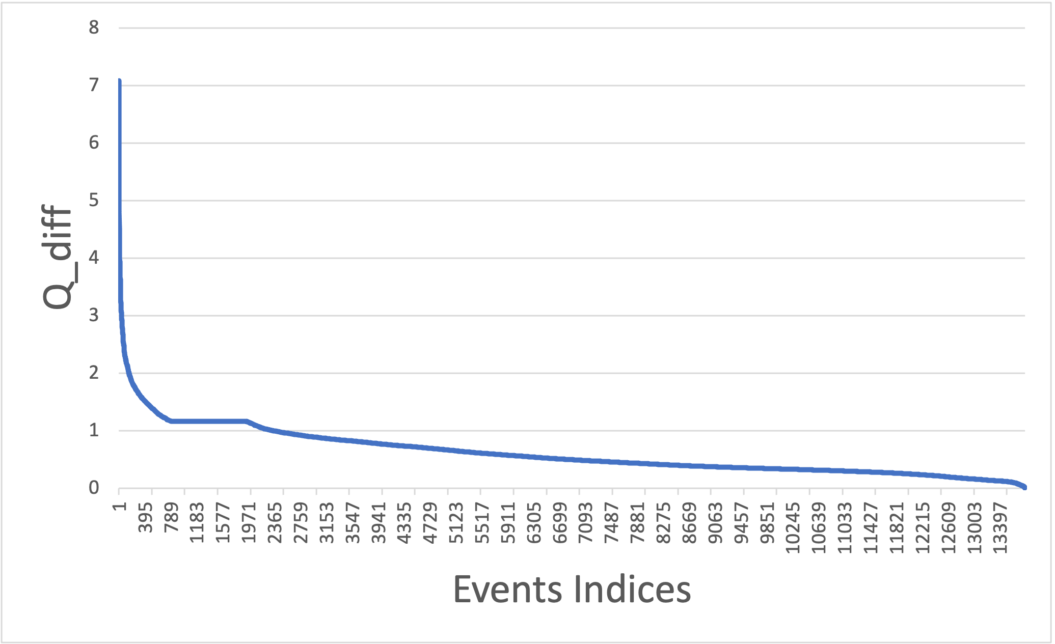
Figure 7. The maximum difference of $Q^{\pi}$ in Intelligent Tutor. We use the elbow method and select $h=1.1$.

Detailed benchmark setting For FQE, we used different convergence $\epsilon=\{1e-3,1e-4,1e-5,4e-3\}$ following Voloshin et al. (2019) and report the one with the least average absolute error (or highest rank correlation). For DualDICE, we used the open-sourced code in its original paper by repeating it three times with different random seeds and report the one with the least average absolute error (or highest rank correlation in real-world medical system).

B.1. Simulation with ICU Patients

The simulator simulated 10000 trajectories. For each OPE, it estimated each policies, including {optimal_policy, with_antibiotics, without_antibiotics} as in Namkoong et al. (2020). Here we computed the OPE estimation for evaluation policy 500 times using bootstrap, and calculated the average value of estimation as well as standard deviations.

B.2. Real-World Medical System

B.2.1. Data Preprocessing

Labels. The hospital provided the EHRs over two years, including 221,700 visits with 35 static variables such as gender, age, and past medical condition, and 43 temporal variables including vital signs, lab analytes, and treatments. Our study population is patients with a suspected infection which was identified by the administration of any type of antibiotic, antiviral, antibacterial, antiparasitic, or antifungal, or a positive test result of PCR (Point of Care Rapid). On the basis of the Third International Consensus Definitions for Sepsis and Septic Shock Singer et al. (2016), our medical experts identified septic shock as any of the following conditions are met:

• Persistent hypertension as shown through two consecutive readings ($\leq$ 30 minutes apart).

• Systolic Blood Pressure (SBP) $<$ 90 mmHg

• Mean Arterial Pressure (MAP) $<$ 65 mmHg

• Decrease in SBP $\geq$ 40 mmHg with an 8-hour period

• Any vasopressor administration.

From the EHRs, 3,499 septic shock positive and 81,398 negative visits were identified based on the intersection of the expert sepsis diagnostic rules and International Codes for Disease 9th division (ICD-9); the 36,122 visits with mismatched labels between the expert rule and the ICD-9 were excluded in our study. 2,205 shock visits were obtained by excluding the visits admitted with septic shock and the long-stay visits and then we did the stratified random sampling from non-shock visits, keeping the same distribution of age, gender, ethnicity, and length of hospital stay. The final data constituted 4,410 visits with an equal ratio of shock and non-shock visits.

Observations. To approximate patient observations, 15 sepsis-related attributes were selected based on the sepsis diagnostic rules. In our data, the average missing rate across the 15 sepsis-related attributes was 78.6%. We avoided deleting sparse attributes or resampling with a regular time interval because the attributes suggested by medical experts are critical to decision making for sepsis treatment, and the temporal missing patterns of EHRs also provide the information of patient observations. The missing values were imputed using Temporal Belief Memory Kim and Chi (2018) combined with missing indicators Lipton et al. (2016).

Actions. For actions, we considered two medical treatments: antibiotic administration and oxygen assistance. Note that the two treatments can be applied simultaneously, which results in a total of four actions. Generally, the treatments are mixed in discrete and continuous action spaces according to their granularity. For example, a decision of whether a certain drug is administrated is discrete, while the dosage of drug is continuous. Continuous action space has been mainly handled by policy-based RL models such as actor-critic models Lillicrap et al. (2015), and it is generally only available for online RL. Since we cannot search continuous action spaces while online interacting with actual patients, we focus on discrete actions. Moreover, in this work, the RL agent aims to let the physicians know when and which treatment should be given to a patient, rather than suggests an optimal amount of drugs or duration of oxygen control that requires more complex consideration.

Rewards. Two leading clinicians, both with over 20-year experience on the subject of sepsis, guided to define the reward function based on the severity of septic stages. The rewards were defined as follows: infection [-5], inflammation [-10], organ failures [-20], and septic shock [-50]. Whenever a patient was recovered from any stage of them, the positive reward for the stage was gained back.

The data was divided into 80% (the earlier 80% according to the time of the first event recorded in patients’ visits) for training and (the later) 20% for test, as the most common task for OPE was using historical data to validate policies then applied selected policies for test.

Policies We estimate the behavior policy with behavior cloning as in Fu et al. (2021); Hanna et al. (2019). The evaluation policies were trained using off-policy DQN algorithm with different learning rates.

B.2.2. Septic Shock Rate.

Since the RL agent cannot directly interact with patients, it only depends on offline data for both policy induction and evaluation. In similar fashion to prior studies Komorowski et al. (2018); Azizsoltani and Jin (2019); Raghu et al. (2017), the induced policies were evaluated using the septic shock rate. The assumption Raghu et al. (2017) behind that is: when a septic shock prevention policy is indeed effective, the more the real treatments in a patient trajectory agree with the induced policy, the lower the chance the patient would get into septic shock; vice versa, the less the real treatments in a patient trajectory agree with the induced policy (more dissimilar), the higher the chance the patient would get into septic shock. Specifically, we measured agreement rate with the agent policy, $a\in[0,1]$ was the number of events agreed with the agent policy among the total number of events in a visit; $a=0$ if the actual treatments and the agent’s recommendations are completely different in a visit trajectory, and $a=1$ if they are the same. According to the agreement rate, the average septic shock rate is calculate, which is the number of shock visits among the visits with the corresponding agreement rate $\geq a$. If the agent policies are indeed effective, the more the actually executed treatments agree with the agent policy, the less likely the patient is going to have septic shock. This metric was first used in Raghu et al. (2017).

B.3. Real-World Intelligent Tutor

B.3.1. Data Collection and Preprocessing

Our data contains a total of 1,307 students’ interaction logs with a web-based ITS collected over seven semesters’ classroom studies. During the studies, all students used the same tutor, followed the same general procedure, studied the same training materials, and worked through the same training problems. All students went through the same four phases: 1) reading textbook, 2) pre-test, 3) working on the ITS, and 4) post-test. During reading textbook, students read a general description of each principle, reviewed examples, and solved some training problems to get familiar with the ITS. Then the students took a pre-test which contained a total of 14 single- and multiple-principle problems. Students were not given feedback on their answers, nor were they allowed to go back to earlier questions (so as the post-test). Next, students worked on the ITS, where they received the same 10 problems in the same order. After that, students took the 20-problem post-test, where 14 of the problems were isomorphic to the pre-test and the remainders were non-isomorphic multiple-principle problems. Tests were auto-graded following the same grading criteria. Test scores were normalized to the range of [0, 1].

Rewards. There was no immediate reward but the empirical evaluation matrix (i.e., delayed reward), which was the students’ Normalized Learning Gain (NLG). NLG measured students’ learning gain irrespective of their incoming competence. NLG is defined as: $NLG=\frac{score_{posttest}-score_{pretest}}{\sqrt{1-score_{pretest}}}$, where 1 denotes the maximum score for both pre- and post-test that were taken before and after usage of the ITS, respectively.

Policies. The study were conducted across seven semesters, where the first six semesters’ data were collected over expert policy and the seventh semester’s data were collected over four different policies (three policies were RL-induced policies and one was the expert policy). The expert policy randomly picked actions. The three RL-induced policies were trained using off-policy DQN algorithm with different learning rates.

References

- (1)
- Abdelshiheed et al. (2021) Mark Abdelshiheed, Mehak Maniktala, Song Ju, Ayush Jain, Tiffany Barnes, and Min Chi. 2021. Preparing Unprepared Students For Future Learning. In Proceedings of the 43rd annual conference of the cognitive science society, Vol. 43.
- Abdelshiheed et al. (2020) Mark Abdelshiheed, Guojing Zhou, Mehak Maniktala, Tiffany Barnes, and Min Chi. 2020. Metacognition and Motivation: The Role of Time-Awareness in Preparation for Future Learning. In Proceedings of the 42nd annual conference of the cognitive science society, Vol. 42.
- Abe and Kaneko (2021) Kenshi Abe and Yusuke Kaneko. 2021. Off-Policy Exploitability-Evaluation in Two-Player Zero-Sum Markov Games. In Proceedings of the 20th International Conference on Autonomous Agents and MultiAgent Systems. 78–87.
- Ausin et al. (2021) Markel Sanz Ausin, Hamoon Azizsoltani, Song Ju, Yeo Jin Kim, and Min Chi. 2021. Infernet for delayed reinforcement tasks: Addressing the temporal credit assignment problem. In 2021 IEEE International Conference on Big Data (Big Data). IEEE, 1337–1348.
- Azizsoltani and Jin (2019) Hamoon Azizsoltani and Yeo Jin. 2019. Unobserved Is Not Equal to Non-existent: Using Gaussian Processes to Infer Immediate Rewards Across Contexts.. In In Proceedings of the 28th International Joint Conference on Artificial Intelligence.
- Bennett et al. (2021) Andrew Bennett, Nathan Kallus, Lihong Li, and Ali Mousavi. 2021. Off-policy evaluation in infinite-horizon reinforcement learning with latent confounders. In International Conference on Artificial Intelligence and Statistics. PMLR, 1999–2007.
- Bone et al. (1992) Roger C Bone, Robert A Balk, Frank B Cerra, R Phillip Dellinger, Alan M Fein, William A Knaus, Roland MH Schein, and William J Sibbald. 1992. Definitions for sepsis and organ failure and guidelines for the use of innovative therapies in sepsis. Chest 101, 6 (1992), 1644–1655.
- Cassandra (1998) Anthony R Cassandra. 1998. A survey of POMDP applications. In Working notes of AAAI 1998 fall symposium on planning with partially observable Markov decision processes, Vol. 1724.
- Chandak et al. (2021) Yash Chandak, Scott Niekum, Bruno da Silva, Erik Learned-Miller, Emma Brunskill, and Philip S Thomas. 2021. Universal off-policy evaluation. Advances in Neural Information Processing Systems 34 (2021).
- Chi et al. (2011) Min Chi, Kurt VanLehn, Diane Litman, and Pamela Jordan. 2011. Empirically evaluating the application of reinforcement learning to the induction of effective and adaptive pedagogical strategies. User Modeling and User-Adapted Interaction 21, 1 (2011), 137–180.
- Doroudi et al. (2017) Shayan Doroudi, Philip S Thomas, and Emma Brunskill. 2017. Importance Sampling for Fair Policy Selection. Grantee Submission (2017).
- Farajtabar et al. (2018) Mehrdad Farajtabar, Yinlam Chow, and Mohammad Ghavamzadeh. 2018. More robust doubly robust off-policy evaluation. In International Conference on Machine Learning. PMLR, 1447–1456.
- Fu et al. (2020) Justin Fu, Aviral Kumar, Ofir Nachum, George Tucker, and Sergey Levine. 2020. D4rl: Datasets for deep data-driven reinforcement learning. arXiv preprint arXiv:2004.07219 (2020).
- Fu et al. (2021) Justin Fu, Mohammad Norouzi, Ofir Nachum, George Tucker, Ziyu Wang, Alexander Novikov, Mengjiao Yang, Michael R Zhang, Yutian Chen, Aviral Kumar, et al. 2021. Benchmarks for deep off-policy evaluation. arXiv preprint arXiv:2103.16596 (2021).
- Gao et al. (2022a) Ge Gao, Qitong Gao, Xi Yang, Miroslav Pajic, and Min Chi. 2022a. A Reinforcement Learning-Informed Pattern Mining Framework for Multivariate Time Series Classification. In International Joint Conference on Artificial Intelligence (IJCAI).
- Gao et al. (2022b) Ge Gao, Farzaneh Khoshnevisan, and Min Chi. 2022b. Reconstructing Missing EHRs Using Time-Aware Within-and Cross-Visit Information for Septic Shock Early Prediction. In 2022 IEEE 10th International Conference on Healthcare Informatics (ICHI). IEEE Computer Society, 151–162.
- Gao et al. (2021) Ge Gao, Samiha Marwan, and Thomas W Price. 2021. Early performance prediction using interpretable patterns in programming process data. In Proceedings of the 52nd ACM Technical Symposium on Computer Science Education. 342–348.
- Gao et al. (2023) Qitong Gao, Ge Gao, Min Chi, and Miroslav Pajic. 2023. Variational Latent Branching Model for Off-Policy Evaluation. In The Eleventh International Conference on Learning Representations.
- Gao et al. (2022c) Qitong Gao, Stephen L Schmidt, Karthik Kamaravelu, Dennis A Turner, Warren M Grill, and Miroslav Pajic. 2022c. Offline Policy Evaluation for Learning-based Deep Brain Stimulation Controllers. In 2022 ACM/IEEE 13th International Conference on Cyber-Physical Systems (ICCPS). IEEE, 80–91.
- Gao et al. (2022d) Qitong Gao, Dong Wang, Joshua D Amason, Siyang Yuan, Chenyang Tao, Ricardo Henao, Majda Hadziahmetovic, Lawrence Carin, and Miroslav Pajic. 2022d. Gradient Importance Learning for Incomplete Observations. International Conference on Learning Representations (2022).
- Gottesman et al. (2020) Omer Gottesman, Joseph Futoma, Yao Liu, Sonali Parbhoo, Leo Celi, Emma Brunskill, and Finale Doshi-Velez. 2020. Interpretable off-policy evaluation in reinforcement learning by highlighting influential transitions. In International Conference on Machine Learning. PMLR, 3658–3667.
- Guilford (1950) Joy Paul Guilford. 1950. Fundamental statistics in psychology and education. (1950).
- Hallac et al. (2017) David Hallac, Sagar Vare, Stephen Boyd, and Jure Leskovec. 2017. Toeplitz inverse covariance-based clustering of multivariate time series data. In Proceedings of the 23rd ACM SIGKDD International Conference on Knowledge Discovery and Data Mining. 215–223.
- Hanna et al. (2019) Josiah Hanna, Scott Niekum, and Peter Stone. 2019. Importance sampling policy evaluation with an estimated behavior policy. In International Conference on Machine Learning. PMLR, 2605–2613.
- Hao et al. (2021) Botao Hao, Xiang Ji, Yaqi Duan, Hao Lu, Csaba Szepesvári, and Mengdi Wang. 2021. Bootstrapping statistical inference for off-policy evaluation. arXiv preprint arXiv:2102.03607 (2021).
- Harutyunyan et al. (2016) Anna Harutyunyan, Marc G Bellemare, Tom Stepleton, and Rémi Munos. 2016. Q(lambda) with Off-Policy Corrections. In International Conference on Algorithmic Learning Theory. Springer, 305–320.
- Horvitz and Thompson (1952) Daniel G Horvitz and Donovan J Thompson. 1952. A generalization of sampling without replacement from a finite universe. Journal of the American statistical Association 47, 260 (1952), 663–685.
- Irpan et al. (2019) Alexander Irpan, Kanishka Rao, Konstantinos Bousmalis, Chris Harris, Julian Ibarz, and Sergey Levine. 2019. Off-policy evaluation via off-policy classification. Advances in Neural Information Processing Systems 32 (2019).
- Jiang (2010) Jiming Jiang. 2010. Large sample techniques for statistics. Springer.
- Jiang and Li (2016) Nan Jiang and Lihong Li. 2016. Doubly robust off-policy value evaluation for reinforcement learning. In International Conference on Machine Learning. PMLR, 652–661.
- Ju et al. (2019) Song Ju, Shitian Shen, Hamoon Azizsoltani, Tiffany Barnes, and Min Chi. 2019. Importance Sampling to Identify Empirically Valid Policies and their Critical Decisions.. In EDM (Workshops). 69–78.
- Keramati et al. (2022) Ramtin Keramati, Omer Gottesman, Leo Anthony Celi, Finale Doshi-Velez, and Emma Brunskill. 2022. Identification of Subgroups With Similar Benefits in Off-Policy Policy Evaluation. In Conference on Health, Inference, and Learning. PMLR, 397–410.
- Khoshnevisan and Chi (2021) Farzaneh Khoshnevisan and Min Chi. 2021. Unifying domain adaptation and domain generalization for robust prediction across minority racial groups. In Joint European Conference on Machine Learning and Knowledge Discovery in Databases. Springer, 521–537.
- Kim and Chi (2018) Yeo-Jin Kim and Min Chi. 2018. Temporal Belief Memory: Imputing Missing Data during RNN Training.. In In Proceedings of the 27th International Joint Conference on Artificial Intelligence (IJCAI-2018).
- Komorowski et al. (2018) Matthieu Komorowski, Leo A Celi, Omar Badawi, Anthony C Gordon, and A Aldo Faisal. 2018. The artificial intelligence clinician learns optimal treatment strategies for sepsis in intensive care. Nature medicine 24, 11 (2018), 1716–1720.
- Kullback and Leibler (1951) Solomon Kullback and Richard A Leibler. 1951. On information and sufficiency. The annals of mathematical statistics 22, 1 (1951), 79–86.
- Le et al. (2019) Hoang Le, Cameron Voloshin, and Yisong Yue. 2019. Batch policy learning under constraints. In International Conference on Machine Learning. PMLR, 3703–3712.
- Lillicrap et al. (2015) Timothy P Lillicrap, Jonathan J Hunt, Alexander Pritzel, Nicolas Heess, Tom Erez, Yuval Tassa, David Silver, and Daan Wierstra. 2015. Continuous control with deep reinforcement learning. arXiv preprint arXiv:1509.02971 (2015).
- Lipton et al. (2016) Zachary C Lipton, David Kale, and Randall Wetzel. 2016. Directly modeling missing data in sequences with rnns: Improved classification of clinical time series. In Machine learning for healthcare conference. PMLR, 253–270.
- Liu et al. (2018) Qiang Liu, Lihong Li, Ziyang Tang, and Dengyong Zhou. 2018. Breaking the curse of horizon: Infinite-horizon off-policy estimation. Advances in Neural Information Processing Systems 31 (2018).
- Liu et al. (2014) Vincent Liu, Gabriel J Escobar, John D Greene, Jay Soule, Alan Whippy, Derek C Angus, and Theodore J Iwashyna. 2014. Hospital deaths in patients with sepsis from 2 independent cohorts. Jama 312, 1 (2014), 90–92.
- Mandel et al. (2014) Travis Mandel, Yun-En Liu, Sergey Levine, Emma Brunskill, and Zoran Popovic. 2014. Offline policy evaluation across representations with applications to educational games.. In AAMAS, Vol. 1077.
- Martin et al. (2003) G.S Martin, D.M Mannino, et al. 2003. The epidemiology of sepsis in the United States from 1979 through 2000. New England Journal of Medicine (2003).
- Marwan et al. (2020) Samiha Marwan, Ge Gao, Susan Fisk, Thomas W Price, and Tiffany Barnes. 2020. Adaptive immediate feedback can improve novice programming engagement and intention to persist in computer science. In Proceedings of the 2020 ACM conference on international computing education research. 194–203.
- Mataric (1994) Maja J Mataric. 1994. Reward functions for accelerated learning. In Machine learning proceedings 1994. Elsevier, 181–189.
- Mnih et al. (2015) Volodymyr Mnih, Koray Kavukcuoglu, David Silver, Andrei A Rusu, Joel Veness, Marc G Bellemare, Alex Graves, Martin Riedmiller, Andreas K Fidjeland, Georg Ostrovski, et al. 2015. Human-level control through deep reinforcement learning. nature 518, 7540 (2015), 529–533.
- Munos et al. (2016) Rémi Munos, Tom Stepleton, Anna Harutyunyan, and Marc Bellemare. 2016. Safe and efficient off-policy reinforcement learning. Advances in neural information processing systems 29 (2016).
- Nachum et al. (2019) Ofir Nachum, Yinlam Chow, Bo Dai, and Lihong Li. 2019. Dualdice: Behavior-agnostic estimation of discounted stationary distribution corrections. Advances in Neural Information Processing Systems 32 (2019).
- Namkoong et al. (2020) Hongseok Namkoong, Ramtin Keramati, Steve Yadlowsky, and Emma Brunskill. 2020. Off-policy policy evaluation for sequential decisions under unobserved confounding. Advances in Neural Information Processing Systems 33 (2020), 18819–18831.
- Nie et al. (2022) Allen Nie, Yannis Flet-Berliac, Deon Richmond Jordan, William Steenbergen, and Emma Brunskill. 2022. Data-Efficient Pipeline for Offline Reinforcement Learning with Limited Data. In Advances in Neural Information Processing Systems.
- Nie et al. (2021) Xinkun Nie, Emma Brunskill, and Stefan Wager. 2021. Learning when-to-treat policies. J. Amer. Statist. Assoc. 116, 533 (2021), 392–409.
- Oberst and Sontag (2019) Michael Oberst and David Sontag. 2019. Counterfactual off-policy evaluation with gumbel-max structural causal models. In International Conference on Machine Learning. PMLR, 4881–4890.
- Paduraru (2013) Cosmin Paduraru. 2013. Off-policy evaluation in Markov decision processes. (2013).
- Payne et al. (2017) Emily Miller Payne, Russ Hodges, and Elda Patricia Hernandez. 2017. Changing Demographics and Needs Assessment for Learning Centers in the 21st Century. Learning Assistance Review 22, 1 (2017), 21–36.
- Powell and Swann (1966) Michael JD Powell and J Swann. 1966. Weighted uniform sampling—a Monte Carlo technique for reducing variance. IMA Journal of Applied Mathematics 2, 3 (1966), 228–236.
- Precup (2000) Doina Precup. 2000. Eligibility traces for off-policy policy evaluation. Computer Science Department Faculty Publication Series (2000), 80.
- Raghu et al. (2017) Aniruddh Raghu, Matthieu Komorowski, Imran Ahmed, Leo Celi, Peter Szolovits, and Marzyeh Ghassemi. 2017. Deep reinforcement learning for sepsis treatment. arXiv preprint arXiv:1711.09602 (2017).
- Rengarajan et al. (2022) Desik Rengarajan, Gargi Vaidya, Akshay Sarvesh, Dileep Kalathil, and Srinivas Shakkottai. 2022. Reinforcement Learning with Sparse Rewards using Guidance from Offline Demonstration. arXiv preprint arXiv:2202.04628 (2022).
- Sen and Singer (1994) Pranab K Sen and Julio M Singer. 1994. Large sample methods in statistics: an introduction with applications. Vol. 25. CRC press.
- Shen and Chi (2016) Shitian Shen and Min Chi. 2016. Reinforcement learning: the sooner the better, or the later the better?. In Proceedings of the 2016 conference on user modeling adaptation and personalization. 37–44.
- Shi et al. (2022) Chengchun Shi, Masatoshi Uehara, Jiawei Huang, and Nan Jiang. 2022. A minimax learning approach to off-policy evaluation in confounded partially observable markov decision processes. In International Conference on Machine Learning. PMLR, 20057–20094.
- Singer et al. (2016) Mervyn Singer, Clifford S Deutschman, Christopher Warren Seymour, Manu Shankar-Hari, Djillali Annane, Michael Bauer, Rinaldo Bellomo, Gordon R Bernard, Jean-Daniel Chiche, Craig M Coopersmith, et al. 2016. The third international consensus definitions for sepsis and septic shock (Sepsis-3). Jama 315, 8 (2016), 801–810.
- Spearman (1987) Charles Spearman. 1987. The proof and measurement of association between two things. The American journal of psychology 100, 3/4 (1987), 441–471.
- Tennenholtz et al. (2020) Guy Tennenholtz, Uri Shalit, and Shie Mannor. 2020. Off-policy evaluation in partially observable environments. In Proceedings of the AAAI Conference on Artificial Intelligence, Vol. 34. 10276–10283.
- Tetreault and Litman (2006) Joel Tetreault and Diane Litman. 2006. Comparing the utility of state features in spoken dialogue using reinforcement learning. In Proceedings of the Human Language Technology Conference of the NAACL, Main Conference. 272–279.
- Thomas and Brunskill (2016) Philip Thomas and Emma Brunskill. 2016. Data-efficient off-policy policy evaluation for reinforcement learning. In International Conference on Machine Learning. PMLR, 2139–2148.
- Thomas (2015) Philip S Thomas. 2015. Safe reinforcement learning. (2015).
- Thomas et al. (2015) Philip S Thomas, Scott Niekum, Georgios Theocharous, and George Konidaris. 2015. Policy evaluation using the Ω-return. Advances in Neural Information Processing Systems 28 (2015).
- Todorov et al. (2012) Emanuel Todorov, Tom Erez, and Yuval Tassa. 2012. Mujoco: A physics engine for model-based control. In 2012 IEEE/RSJ international conference on intelligent robots and systems. IEEE, 5026–5033.
- Torrey and Taylor (2013) Lisa Torrey and Matthew Taylor. 2013. Teaching on a budget: Agents advising agents in reinforcement learning. In Proceedings of the 2013 international conference on Autonomous agents and multi-agent systems. 1053–1060.
- Uehara et al. (2020) Masatoshi Uehara, Jiawei Huang, and Nan Jiang. 2020. Minimax weight and q-function learning for off-policy evaluation. In International Conference on Machine Learning. PMLR, 9659–9668.
- Uehara et al. (2022) Masatoshi Uehara, Haruka Kiyohara, Andrew Bennett, Victor Chernozhukov, Nan Jiang, Nathan Kallus, Chengchun Shi, and Wen Sun. 2022. Future-Dependent Value-Based Off-Policy Evaluation in POMDPs. arXiv preprint arXiv:2207.13081 (2022).
- VanLehn (2006) Kurt VanLehn. 2006. The Behavior of Tutoring Systems. International Journal Artificial Intelligence in Education 16, 3 (2006), 227–265.
- Voloshin et al. (2019) Cameron Voloshin, Hoang M Le, Nan Jiang, and Yisong Yue. 2019. Empirical study of off-policy policy evaluation for reinforcement learning. arXiv preprint arXiv:1911.06854 (2019).
- Xie et al. (2019) Tengyang Xie, Yifei Ma, and Yu-Xiang Wang. 2019. Towards optimal off-policy evaluation for reinforcement learning with marginalized importance sampling. Advances in Neural Information Processing Systems 32 (2019).
- Yang et al. (2022) Mengjiao Yang, Bo Dai, Ofir Nachum, George Tucker, and Dale Schuurmans. 2022. Offline policy selection under uncertainty. In International Conference on Artificial Intelligence and Statistics. PMLR, 4376–4396.
- Yang et al. (2021) Xi Yang, Yuan Zhang, and Min Chi. 2021. Multi-series time-aware sequence partitioning for disease progression modeling. In IJCAI.
- Yang et al. (2020) Xi Yang, Guojing Zhou, Michelle Taub, Roger Azevedo, and Min Chi. 2020. Student Subtyping via EM-Inverse Reinforcement Learning. International Educational Data Mining Society (2020).
- Yin et al. (2020) Changchang Yin, Ruoqi Liu, Dongdong Zhang, and Ping Zhang. 2020. Identifying sepsis subphenotypes via time-aware multi-modal auto-encoder. In Proceedings of the 26th ACM SIGKDD international conference on knowledge discovery & data mining. 862–872.
- Zhou et al. (2022) Guojing Zhou, Hamoon Azizsoltani, Markel Sanz Ausin, Tiffany Barnes, and Min Chi. 2022. Leveraging granularity: Hierarchical reinforcement learning for pedagogical policy induction. International journal of artificial intelligence in education 32, 2 (2022), 454–500.
- Zhou et al. (2020) Guojing Zhou, Xi Yang, Hamoon Azizsoltani, Tiffany Barnes, and Min Chi. 2020. Improving student-system interaction through data-driven explanations of hierarchical reinforcement learning induced pedagogical policies. In Proceedings of the 28th ACM Conference on User Modeling, Adaptation and Personalization. 284–292.