Bayesian Covariance Estimation for Multi-group Matrix-variate Data

Abstract

Multi-group covariance estimation for matrix-variate data with small within-group sample sizes is a key part of many data analysis tasks in modern applications. To obtain accurate group-specific covariance estimates, shrinkage estimation methods which shrink an unstructured, group-specific covariance either across groups towards a pooled covariance or within each group towards a Kronecker structure have been developed. However, in many applications, it is unclear which approach will result in more accurate covariance estimates. In this article, we present a hierarchical prior distribution which flexibly allows for both types of shrinkage. The prior linearly combines shrinkage across groups towards a shared pooled covariance and shrinkage within groups towards a group-specific Kronecker covariance. We illustrate the utility of the proposed prior in speech recognition and an analysis of chemical exposure data.

and

1 Introduction

Matrix-variate datasets consisting of a sample of $n$ matrices $Y_{1},...,Y_{n}$ each with dimensionality $p_{1}\times p_{2}$ are increasingly common in modern applications. Examples of such datasets include repeated measurements of a multivariate response, two-dimensional images, and spatio-temporal observations. Often, a matrix-variate dataset may be partitioned into several distinct groups or subpopulations for which group-level inference is of particular interest. For example, a multi-group dataset may be subdivided by socio-economic population or geographic region.

In analyzing multi-group matrix-variate data of this type, describing heterogeneity across groups is often of particular interest. For instance, in remote-sensing studies, scientists may be interested in understanding variation across classes of land cover from repeated measurements of spectral information, as in Johnson et al. (2012). The information collected at each site may be represented as a $p_{1}\times p_{2}$ matrix where the rows represent $p_{1}$ wavelengths and the columns represent $p_{2}$ dates when the images were taken. Accurate multi-group covariance estimation is necessary for such a task. Moreover, in many such applications, the population covariance of matrix-variate data may be near separable in that the covariances across the $p_{2}$ columns are near each other or the covariances across the $p_{1}$ rows are near each other. Incorporation of this structural information in an estimation procedure can improve estimation accuracy. More generally, accurate covariance estimation of multi-group, matrix-variate data is a pertinent task in many statistical methodologies including classification, principal component analysis, and multivariate regression analysis, among others. For example, classification of a new observation based on a labeled training dataset with quadratic discriminant analysis (QDA) requires group-level estimates of population means and covariance matrices. As a result, adequate performance of the classification relies on, among other things, accurate group-level covariance estimates.

One approach to analyzing multi-group matrix-variate data is to vectorize each data matrix and utilize methods designed for generic multivariate data separately for each group. In this way, direct covariance estimates which only make use of within-group samples may be obtained from matrix-variate data by vectorizing each observation and computing the standard sample covariance matrices. While a group’s sample covariance may be unbiased, the estimate may have large variance unless the group-specific sample size $n_{j}$ is appreciably larger than the dimension $p=p_{1}p_{2}$. This is a limiting requirement as modern datasets often consist of many features, that is, often $p\approx n_{j}$, or even $p\gg n_{j}$. As a result, more accurate covariance estimates may be obtained via indirect or model-based methods which incorporate auxiliary information. Such methods may introduce bias, but can correspond to estimates with lower variance than unbiased methods.

To improve the accuracy of covariance estimates for multi-group data, researchers may estimate each group’s covariance with the pooled sample covariance matrix. This implicitly imposes an assumption of homogeneity of covariances across the populations and greatly reduces the number of unknown parameters to be estimated. Such an estimator may be biased, but can have lower error than the population-specific sample covariance. For example, linear discriminant analysis (LDA), which assumes homoscedasticity across groups, has been shown to outperform QDA when sample sizes are small, even in the presence of heterogeneous population covariances (see, for example, Marks and Dunn (1974)). A more robust approach estimates each group’s covariance as a weighted sum of a pooled estimate and the group-specific sample covariance. Such an approach is often referred to as partial-pooling, or, in the Bayesian framework, hierarchical modeling. For a nice introduction to partial pooling and an empirical Bayesian implementation, see Greene and Rayens (1989). More work on the topic is found in Friedman (1989); Rayens and Greene (1991); Brown et al. (1999). Relatedly, there has been work which assumes pooled elements of common covariance decompositions (e.g. pooled eigenvectors across groups (Flury, 1987)) and proposals to shrink elements of decompositions to pooled values (Daniels, 2006; Hoff, 2009).

Alternatively, as opposed to pooling information across groups, accuracy may be improved by imposing structural assumptions on the covariances separately for each group. Some common structural assumptions include diagonality (Daniels and Kass, 1999), bandability (Wu and Pourahmadi, 2009), and sparsity (Friedman et al., 2008), among others. For matrix-variate data, a separable or Kronecker structure covariance assumption (Dawid, 1981) may be more appropriate. A Kronecker structured covariance represents each $p\times p$ population covariance as the Kronecker product of two smaller covariance matrices of dimension $p_{1}\times p_{1}$ and $p_{2}\times p_{2}$ which respectively represent the across-row and across-column covariances. Again, while a separable covariance estimator may be biased, it may have smaller error than an unstructured covariance estimator. In practice, however, the population covariance may not be well represented by a Kronecker structure. To allow for robustness to misspecification, a researcher may proceed in a Bayesian manner and adaptively shrink to the Kronecker structure as in Hoff et al. (2022). Such an estimator can be consistent, but may have stability issues similar to that of an unstructured covariance matrix if the population covariance is not well represented by a Kronecker structure. In this instance, more accurate multi-group covariance estimates may be obtained by pooling across groups rather than shrinking within each group to a separable structure.

More generally, in covariance estimation based on matrix-variate data from multiple populations, it is rarely obvious whether shrinking each unstructured covariance separately towards a Kronecker structure or shrinking all unstructured covariances towards an unstructured pooled covariance will result in more accurate estimates. This is particularly difficult in the presence of small within-group sample sizes as popular classical statistical tests for both homogeneity of covariances (Box, 1949) and accuracy of a Kronecker structure assumption (Lu and Zimmerman, 2005) rely on approximations that require large sample sizes to achieve the desired precision.

To account for this uncertainty, we propose a hierarchical model that adaptively allows for both types of shrinkage. Specifically, in this article, we provide a model-based multi-group covariance estimation method for matrix-variate data that improves the overall accuracy of direct covariance estimates. We propose a hierarchical model for unstructured group-level covariances that adaptively shrinks each estimate either within-population towards a separable Kronecker structure, across-populations towards a shared pooled covariance, or towards a weighted additive combination of the two. The model features flexibility in the amount of each type of shrinkage. Furthermore, the proposed model has a latent-variable representation that results in straightforward Bayesian inference via a Metropolis-Hastings algorithm. The proposed model provides robustness to mis-specification of structural assum ptions and improved stability if assumptions are wrong while maintaining coherence and interpretability.

The article proceeds as follows. In Section 2 we motivate our method and detail the proposed hierarchical model. We describe a Bayesian estimation algorithm in Section 3 and demonstrate properties of the proposed method via a simulation study in Section 4. The flexibility of the proposed method is shown in two examples in Section 5. In the first example, we demonstrate the usefulness of inference under the proposed model in speech recognition. In the second example, we perform inference on a chemical exposure data set where understanding heterogeneity across socio-demographic groups is of key interest. We conclude with a discussion in Section 6.

2 Methodology

In this section we introduce the Shrinkage Within and Across Groups (SWAG) covariance model, a hierarchical model developed for simultaneous covariance estimation for multi-group, matrix-variate data. We are particularly motivated by improving the overall accuracy of group-specific estimates of population covariances when the true covariance structures are unknown and group-specific sample sizes are small relative to the number of features. The proposed model adaptively allows for flexible shrinkage either across groups, within a group to a Kronecker structure, or an additive combination of the two. The SWAG model is constructed from semi-conjugate priors to allow for straightforward Bayesian estimation and interpretable parameters. The section proceeds by introducing motivation in Sections 2.1 and 2.2, presenting the proposed hierarchical covariance model in Section 2.3, and elaborating on parameter interpretation in Section 2.4.

2.1 Partial-pooling shrinkage for multi-group data

As detailed in the Introduction, a common method used to improve a population’s covariance estimate is linear shrinkage from the population’s sample covariance matrix towards some covariance term which can be estimated with greater precision. One such method for multi-group multivariate data is partial pooling, as detailed in Greene and Rayens (1989, GR). In particular, for population $j\in\{1,...,J\}$, let $y_{1,j},...,y_{n_{j},j}$ be an i.i.d. random sample of $p$-dimensional vectors from a mean-zero normal population with unknown non-singular covariance matrix $\Sigma_{j}\in\mathcal{S}^{+}_{p}$,

$$y_{1,j},...,y_{n_{j},j}\sim N_{p}\left(0,\Sigma_{j}\right),\quad\text{independently for }i=1,...,n_{j},\;j=1,...,J.$$

GR use mutually independent inverse-Wishart priors for each population covariance,
$\Sigma_{j}^{-1}\sim\text{Wishart}_{p}\big{(}\Psi_{0}^{-1}/(\nu-p-1),\nu\big{)},$ for $j\in\{1,...,J\}$, parameterized such that $E[\Sigma_{j}|\Psi_{0},\nu]=\Psi_{0}$. The Bayes estimator for the covariance of population $j$ under squared error loss partially-pools each group’s sample covariance,

$$\hat{\Sigma}_{j}:=E\left[\Sigma_{j}|\boldsymbol{y},\Psi_{0},\nu\right]=w_{1}S_{j}+(1-w_{1}){\Psi}_{0},$$ (1)

where $w_{1}=n_{j}/(n_{j}+{\nu}-p-1)$ and $S_{j}=\sum_{i=1}^{n_{j}}y_{i,j}y_{i,j}^{T}/n_{j}$ is the sample covariance matrix for population $j$. GR use plug-in estimates for the pooled covariance and degrees of freedom $\{\Psi_{0},\nu\}$ which are obtained in an empirical Bayesian manner.

This partially-pooled estimator linearly shrinks a population’s sample covariance matrix towards a pooled covariance by a weight $w_{1}$ that depends on the degrees of freedom and the group-specific sample size $n_{j}$. In this way, the degrees of freedom parameter determines the amount of shrinkage towards the pooled covariance. In particular, if the degrees of freedom $\nu$ is large relative to the sample size $n_{j}$, the covariance estimate is strongly shrunk towards the pooled value. In populations where the group-specific sample size is large, or if the degrees of freedom estimate is comparatively small, more weight is placed on the sample covariance matrix.

2.2 Kronecker shrinkage for matrix-variate data

For a matrix-variate population, the accuracy of a covariance estimate may be improved via linear shrinkage towards a population-specific Kronecker structure. Let $Y_{1},...,Y_{n}$ be an i.i.d. sample of random matrices, each of dimension $p_{1}\times p_{2}$ , from a mean-zero normal population with non-singular covariance matrix $\Sigma\in\mathcal{S}^{+}_{p}$ where $p=p_{1}p_{2}$,

$$Y_{1},...,Y_{n}\sim N_{p_{1}\times p_{2}}\left(0,\Sigma\right),\quad\text{independently for }i=1,...,n.$$

Even if $p_{1}$ and $p_{2}$ are each relatively small, obtaining a statistically stable estimate of the unstructured $p$-dimensional covariance may require a prohibitively large sample size. As a result, shrinkage towards a parsimonious Kronecker structured covariance $C\,\otimes\,R$ may be used, where “$\,\otimes\,$” is the Kronecker product, $R\in\mathcal{S}^{+}_{p_{1}}$ is a “row” covariance matrix, and $C\in\mathcal{S}^{+}_{p_{2}}$ is a “column” covariance matrix. A linear shrinkage estimator that shrinks a population’s sample covariance towards a population-specific Kronecker separable covariance may be obtained from the following prior,

$$\Sigma^{-1}\sim\text{Wishart}_{p}\left(\left(C\,\otimes\,R\right)^{-1}/(\gamma-p-1),\gamma\right),$$

parameterized so that $E[\Sigma_{j}|C,R,\gamma]=C\,\otimes\,R$. Here, the Bayes estimator of the covariance $\Sigma$ under squared error loss is

$$\hat{\Sigma}:=E\left[\Sigma|\boldsymbol{Y},C,R,\gamma\right]=w_{2}S+(1-w_{2})\left({C}\,\otimes\,{R}\right),$$ (2)

where $w_{2}=n/(n+{\gamma}-p-1)$. An empirical Bayesian estimation approach based on shrinkage towards a Kronecker structure is presented in Hoff et al. (2022). In context to that article, here, we will take a fully Bayesian approach.

The estimator given in Equation 2 linearly shrinks the unstructured sample covariance towards a Kronecker structured covariance by the weight $w_{2}$ that depends on the sample size and the estimated degrees of freedom. As with the partially-pooled estimator, this estimator is strongly shrunk towards the Kronecker structure when the degrees of freedom is large relative to sample size. If the degrees of freedom is small, or the sample size is large, more weight is placed on the sample covariance.

2.3 Flexible shrinkage for multi-group matrix-variate data

For each group $j=1,...,J$, let $Y_{j,1},...,Y_{j,n_{j}}$ be an i.i.d. sample of random matrices, each of dimension $p_{1}\times p_{2}$, from a mean-zero normal population with non-singular covariance $\Sigma_{j}\in\mathcal{S}^{+}_{p}$, that is,

$$Y_{j,1},...,Y_{j,n_{j}}\sim N_{p_{1}\times p_{2}}\left(0,\Sigma_{j}\right),\quad\text{independently for }j=1,...,J.$$ (3)

As it is often unclear which of the approaches presented is most appropriate in the presence of multi-group matrix-variate data of this type, we propose an approach that combines the two methods of covariance shrinkage discussed. In particular, we propose the Shrinkage Within and Across Groups (SWAG) hierarchical prior distribution which linearly combines an estimate shrunk towards a pooled covariance $\Psi_{0}$ and an estimate shrunk towards a group-specific Kronecker structure $\left(C_{j}\,\otimes\,R_{j}\right)$ by a weight $\lambda\in[0,1]$ that is estimated from the data.

Specifically, the SWAG prior utilizes an over-parameterized representation of each group’s covariance. That is, for population $j\in\{1,...,J\}$,

$$\Sigma_{j}={} \lambda\Psi_{j}+(1-\lambda)\Lambda_{j},$$ (4)

where each $\Psi_{j}$ is shrunk towards a common covariance, and each $\Lambda_{j}$ is shrunk towards a group specific Kronecker covariance. Each covariance $\Psi_{j}$ is shrunk across groups towards a common covariance matrix using the prior distribution

$$\Psi_{j}^{-1}\sim{} \text{Wishart}_{p}\left(\Psi_{0}^{-1}/(\nu-p-1),\nu\right),\quad\text{independently for }j=1,...,J,$$ (5)

parameterized such that $E[\Psi_{j}|\Psi_{0},\nu]=\Psi_{0}$. When $\Psi_{0}$ is estimated from data across all groups, this term is interpreted as a pooled covariance matrix. As we are interested in obtaining a covariance matrix estimate based on matrix-variate data, each $\Lambda_{j}$ term is shrunk towards a group-specific Kronecker structured covariance,

$$\Lambda_{j}^{-1}\sim{} \text{Wishart}_{p}\left(\left(C_{j}\,\otimes\,R_{j}\right)^{-1}/(\gamma-p-1),\gamma\right),\quad\text{independently for }j=1,...,J,$$ (6)

where $E[\Lambda_{j}|R_{j},C_{j},\gamma]=\left(C_{j}\,\otimes\,R_{j}\right)$. Here, as before, $R_{j}$ is a $p_{1}\times p_{1}$ row covariance matrix from population $j$ and $C_{j}$ is the corresponding $p_{2}\times p_{2}$ column covariance matrix. Furthermore, to more clearly separate these two notions of shrinkage (within population or across populations), a Wishart prior on the across-population covariance $\Psi_{0}$ allows for flexible shrinkage of this pooled term towards an across-group Kronecker covariance:

$$\Psi_{0}\sim\text{Wishart}_{p}\left(\left(P_{2}\,\otimes\,P_{1}\right)/\xi,\xi\right),$$ (7)

parameterized such that $E\left[\Psi_{0}|P_{1},P_{2},\xi\right]=\left(P_{2}\,\otimes\,P_{1}\right)$ where $P_{1}\in\mathcal{S}^{+}_{p_{1}}$ and $P_{2}\in\mathcal{S}^{+}_{p_{2}}$. In this way, the weight $\lambda$ is interpreted as partially controlling the amount of shrinkage towards homogeneity versus towards heterogeneity of covariances across groups. A visualization of the proposed SWAG hierarchy is given in Figure 1. In summary, the SWAG model combines a standard hierarchical model on the across-group shrunk $\Psi_{j}$ covariances with Bayesian shrinkage towards a separable structure on the within-group shrunk $\Lambda_{j}$ covariances and the pooled covariance $\Psi_{0}$.

We note that the SWAG model is primarily motivated by the need to obtain more accurate group-specific covariance estimates, so, while there is redundancy in this parameterization, the group-specific covariances $\Sigma_{1},...,\Sigma_{J}$ are identifiable. As a result, this over-parameterization will not affect inference on estimation of group-level covariances, estimation of mean effects, imputation of missing data, or response prediction.

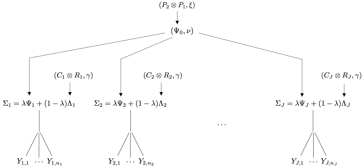
Figure 1: A graphical representation of the SWAG hierarchical model. The unstructured covariance terms $\Psi_{1},...,\Psi_{J}$ are shrunk across groups towards a shared covariance $\Psi_{0}$. The covariance terms $\Psi_{0},\Lambda_{1},....\Lambda_{J}$ are each individually shrunk towards a Kronecker covariance.

2.4 Interpretation of Parameters

In this section, we highlight properties of the proposed SWAG covariance priors under the normal sampling model given in Equation 3. A priori, regardless of the specified sampling model, the marginal expectation under the SWAG prior is a weighted sum of a pooled covariance and the heterogeneous Kronecker separable covariance:

$$E\left[\Sigma_{j}|\Psi_{0},R_{j},C_{j},\lambda\right]=\lambda\Psi_{0}+(1-\lambda)\left(C_{j}\,\otimes\,R_{j}\right),$$ (8)

for $j\in\{1,...,J\}$, where the weight $\lambda$ quantifies the prior weight on each structure. As a result, the SWAG prior presents a flexible approach to combine shrinkage across groups towards a pooled value and shrinkage within groups towards a separable structure.

The role of the weight $\lambda$ is further elucidated at the extremes of its sample space. Given $\lambda=1$, the SWAG model reduces to a Bayesian analogue of the partially-pooled estimators given in Greene and Rayens (1989), as given in Equation 1. At the weight’s opposite extreme, when $\lambda=0$, the SWAG model is equivalent to the Kronecker structure shrinkage model presented in Section 2.2 applied separately to each group. To alleviate some of the potential ambiguity in interpretation of $\lambda$, we further allow $\Psi_{0}$ to be flexibly shrunk to a Kronecker structure. In this way, $\lambda=1$ represents hierarchical shrinkage across populations towards a pooled covariance and $\lambda=0$ represents within-population shrinkage.

Moreover, under the SWAG prior, the prior marginal expected value of a population’s covariance is a weighted sum of a pooled covariance and a population-specific separable covariance (Equation 8). Under normality, as the degrees of freedom $\nu$ and $\gamma$ increase, the marginal sampling model of a random matrix $Y_{i,j}$ converges to a normal distribution with this prior expectation as the covariance. That is, when the degrees of freedom parameters $\nu$ and $\gamma$ are large, the unstructured covariances $\Psi_{j}$ and $\Lambda_{j}$ are each strongly shrunk towards their respective prior expected value, and, therefore, the population covariances are approximately represented by the weighted sum of the pooled covariance and population-specific Kronecker structure.

3 Parameter Estimation

3.1 Latent Variable Representation

The SWAG model has a latent variable representation that allows for straightforward Bayesian inference. Specifically, consider the following representation of the proposed SWAG model:

$$vec(Y_{i,j})={} \lambda^{1/2}U_{i,j}+(1-\lambda)^{1/2}E_{i,j},\quad\text{for }i=1,...,n_{j}$$ (9)

$$U_{i,j}\sim{} N_{p}\left(0,\Psi_{j}\right)$$

$$E_{i,j}\sim{} N_{p}\left(0,\Lambda_{j}\right),$$

independently for each population $j\in\{1,...,J\}$ where the priors on each $\Psi_{j}$ and $\Lambda_{j}$ are as given in Equations 5 and 6. That is, each matrix $Y_{i,j}$ is represented as a weighted sum of one factor ($U_{i,j}$) which partially pools covariances across populations and another factor ($E_{i,j}$) which flexibly shrinks the population covariance towards a group-specific Kronecker structure. Marginal with respect to the factors, this latent variable representation is equivalent to the sampling model proposed in the SWAG model,

$$vec(Y_{i,j})|\lambda,\Psi_{j},\Lambda_{j}\sim N_{p}\left(0,\lambda\Psi_{j}+(1-\lambda)\Lambda_{j}\right).$$

Conditioning on the factor $U_{i,j}$ results in closed form full conditionals of the covariance parameters of interest, as detailed in subsequent subsections.

3.2 Posterior Approximation

In this section, we detail a Metropolis-Hastings algorithm for parameter estimation based on the latent variable representation of the SWAG model. Label $\boldsymbol{Y}=\{Y_{i,j}:i\in\{1,...,n_{j}\},j\in\{1,...,J\}\}$, $\boldsymbol{U}=\left\{U_{i,j}:i\in\{1,...,n_{j}\},j\in\{1,...,J\}\right\}$, $\boldsymbol{\Psi}=\{\Psi_{1},...,\Psi_{J}\}$, $\boldsymbol{\Lambda}=\{\Lambda_{1},...,\Lambda_{J}\}$, $\boldsymbol{R}=\{R_{1},...,R_{J}\}$, and $\boldsymbol{C}=\{C_{1},...,C_{J}\}$. Then, Bayesian inference is based on the joint posterior distribution, with density

$$p(\lambda,\boldsymbol{\Psi},\boldsymbol{\Lambda},\Psi_{0},\nu,\boldsymbol{R},\boldsymbol{C},\gamma,P_{1},P_{2},\xi|\boldsymbol{Y}),$$

and a Monte Carlo approximation to this posterior distribution is available via a MetropolisHastings algorithm. Based on the latent variable representation presented in Equations 9, all but one of the parameters in the SWAG model maintain semi-conjugacy leading to a straightforward Metropolis-Hastings algorithm which constructs a Markov chain in

$$\boldsymbol{\theta}=\{\lambda,\boldsymbol{\Psi},\boldsymbol{\Lambda},\boldsymbol{U},\Psi_{0},\nu,\boldsymbol{R},\boldsymbol{C},\gamma,P_{1},P_{2},\xi\}.$$

Such Bayesian inference provides estimates and uncertainty quantification for arbitrary functions of the parameters. While we focus on the mean-zero case, the algorithm presented may be trivially extended to include estimation of mean parameters.

For a full Bayesian analysis, priors must be specified for all unknown parameters. For simplicity, a straightforward $beta(\alpha,\beta)$ prior may be used to describe prior expectations of behavior of $\lambda$. On the degrees of freedom $\nu,\gamma,$ and $\xi$, we use discrete uniform prior distributions on the sample space $\{p+2,p+3,...,p+K\}$ for some large value $K$. Semi-conjugate priors on the remaining covariance parameters are proposed to facilitate computation,

$$R_{1},...,R_{J}\sim{} \text{Wishart}_{p_{1}}\left(R_{0}/\eta_{1},\eta_{1}\right)$$

$$C_{1},...,C_{J}\sim{} \text{Wishart}_{p_{2}}\left(C_{0}/\eta_{2},\eta_{2}\right)$$

$$P_{1}^{-1}\sim{} \text{Wishart}_{p_{1}}\left(P_{01}^{-1}/(\eta_{3}-p_{1}-1),\eta_{3}\right)$$

$$P_{2}^{-1}\sim{} \text{Wishart}_{p_{2}}\left(P_{02}^{-1}/(\eta_{4}-p_{1}-1),\eta_{4}\right).$$

A Metropolis-Hastings sampler proceeds by iteratively sampling each model parameter from its full conditional distribution. When iterated until convergence, this procedure will generate a Markov chain that approximates the joint posterior distribution $p(\boldsymbol{\theta}|\boldsymbol{Y})$. The full conditionals are now detailed.

3.2.1 Full conditionals of sampling model parameters

The full conditionals of sampling model covariances and factors, as well as the key shrinkage controlling parameters $\lambda,\nu,\gamma$ are discussed in this subsection. To reduce dependence along the Markov chain, we propose to sample the weight $\lambda$ and the latent factor $\boldsymbol{U}$ from their joint full conditional distribution, $p(\lambda,\boldsymbol{U}|\boldsymbol{Y},\boldsymbol{\theta}_{-\boldsymbol{U},-\lambda})$, where, to streamline notation, we let $\boldsymbol{\theta}_{-(\cdot)}$ denote the set containing all variables in $\boldsymbol{\theta}$ except for $(\cdot)$. A sample from $p(\lambda|\boldsymbol{Y},\boldsymbol{\theta}_{-\boldsymbol{U},-\lambda})$ must first be obtained where

$$p(\lambda|\boldsymbol{Y},\boldsymbol{\theta}_{-\boldsymbol{U},-\lambda})\propto\prod_{j=1}^{J}[\left|\lambda\Psi_{j}+(1-\lambda)\Lambda_{j}\right|^{-n_{j}/2}e^{tr(-Y_{j}\left(\lambda\Psi_{j}+(1-\lambda)\Lambda_{j}\right)^{-1}Y_{j}^{T})}]\lambda^{\alpha-1}(1-\lambda)^{\beta-1}.$$

As the conditional distribution of $\lambda$ is not available in closed form, a sample of $\lambda$ may be obtained from a Metropolis proposal. Specifically, a Metropolis step proceeds by first obtaining a proposal sample $\lambda^{*}$ from a reflecting random walk around the previous sample of $\lambda$ in the Markov chain. This proposal is accepted as an updated sample with probability $r=p(\lambda^{*}|\boldsymbol{Y},\boldsymbol{\theta}_{-\boldsymbol{U},-\lambda})/p(\lambda|\boldsymbol{Y},\boldsymbol{\theta}_{-\boldsymbol{U},-\lambda})$. The full conditional of each latent factor $U_{j}$ for population $j$ is independently $N_{n_{j}\times p}\left(M_{j},S_{j}\,\otimes\,I_{n_{j}}\right)$ where

$$S_{j}={} \left(\Psi_{j}^{-1}+\frac{\lambda}{1-\lambda}\Lambda_{j}^{-1}\right)^{-1}$$

$$M_{j}={} \frac{\lambda^{1/2}}{1-\lambda}Y_{j}\Lambda_{j}^{-1}S_{j}.$$

Again, to reduce dependence along the Markov chain, we propose to sample the degrees of freedom $\nu$ and covariances $\boldsymbol{\Psi}$ as well as $\gamma$ and $\boldsymbol{\Lambda}$ from their joint full conditional distributions. In particular, the joint full conditional of $(\nu,\boldsymbol{\Psi})$ is $p(\nu,\boldsymbol{\Psi}|\boldsymbol{Y},\boldsymbol{\theta}_{-\boldsymbol{\Psi},-\nu})=p\left(\boldsymbol{\Psi}|\boldsymbol{Y},\boldsymbol{\theta}_{-\boldsymbol{\Psi}}\right)p\left(\nu|\boldsymbol{Y},\boldsymbol{\theta}_{-\boldsymbol{\Psi},-\nu}\right)$ where

$$P\left(\nu=\nu^{*}|\boldsymbol{Y},\boldsymbol{\theta}_{-\boldsymbol{\Psi},-\nu}\right)=\frac{\prod_{j=1}^{J}p\left(U_{j}|\Psi_{0},\nu=\nu^{*}\right)}{\sum_{\nu^{{}^{\prime}}=p+2}^{p+k}\prod_{j=1}^{J}p\left(U_{j}|\Psi_{0},\nu=\nu^{{}^{\prime}}\right)},\;\nu^{*}\in\{p+2,...,p+K\},$$

for $U_{j}|\Psi_{0},\nu\sim\text{T}_{n_{j}\times p}\left(\nu-p+1,0,\Psi_{0}(\nu-p-1)\,\otimes\,I_{n_{j}}\right)$, and

$$\Psi_{j}^{-1}|\boldsymbol{Y},\boldsymbol{\theta}_{-\Psi_{j}}\sim\text{Wishart}_{p}\big{(}\left(U_{j}^{T}U_{j}+(\nu-p-1)\Psi_{0}\right)^{-1},\nu+n_{j}\big{)}$$

for each $j\in\{1,...,J\}$. Similarly, the joint full conditional of $(\gamma,\boldsymbol{\Lambda})$ is $p(\boldsymbol{\Lambda}|\boldsymbol{Y},\boldsymbol{\theta}_{-\boldsymbol{\Lambda}})$ $\times$ $p\left(\gamma|\boldsymbol{Y},\boldsymbol{\theta}_{-\boldsymbol{\Lambda},-\gamma}\right)$ where

$$P\left(\gamma=\gamma^{*}|\boldsymbol{Y},\boldsymbol{\theta}_{-\boldsymbol{\Lambda},-\gamma}\right)=\frac{\prod_{j=1}^{J}p\left(Y_{j}|\lambda,U_{j},R_{j},C_{j},\gamma=\gamma^{*}\right)}{\sum_{\gamma^{{}^{\prime}}=p+2}^{p+k}\prod_{j=1}^{J}p\left(Y_{j}|\lambda,U_{j},R_{j},C_{j},\gamma=\gamma^{{}^{\prime}}\right)},\;\gamma^{*}\in\{p+2,...,p+K\},$$

for $Y_{j}|\lambda,R_{j},C_{j}\sim T_{n_{j}\times p}\left(\gamma-p+1,\lambda^{1/2}U_{j},(1-\lambda)\left(C_{j}\,\otimes\,R_{j}\right)(\gamma-p-1)\,\otimes\,I_{n_{j}}\right)$, and the full conditional of each $\Lambda_{j}^{-1}$ is independently $\text{Wishart}_{p}\big{(}\big{(}\tilde{Y}_{j}^{T}\tilde{Y}_{j}/(1-\lambda)+\left(C_{j}\,\otimes\,R_{j}\right)(\gamma-p-1)\big{)}^{-1},\gamma+n_{j}\big{)}$ where $\tilde{Y}_{j}=\left(Y_{j}-\lambda^{1/2}U_{j}\right)$.

In addition to facilitating computation, these full conditionals contribute to the interpretation of parameters. In particular, for population $j\in\{1,...,J\}$, the full conditional means of $\Psi_{j}$ and $\Lambda_{j}$ resemble shrinkage estimators towards a pooled covariance and a Kronecker structured covariance, respectively. Specifically, the full conditional density of the across-group shrunk covariance $\Psi_{j}$, given all other model parameters and the observed data matrices $\boldsymbol{Y}$, is inverse-Wishart with mean

$$E\left[\Psi_{j}|\boldsymbol{Y},\boldsymbol{\theta}_{-\Psi_{j}}\right]={} w_{1}U_{j}^{T}U_{j}/n_{j}+(1-w_{1})\Psi_{0},$$

where $w_{1}=n_{j}/(n_{j}+\nu-p-1)$. That is, the prior on $\Psi_{j}$ shrinks the sample covariance of the latent factor $U$ towards the pooled covariance by a shrinkage factor determined by the degrees of freedom $\nu$. Similarly, the full conditional density of the within-group shrunk $\Lambda_{j}$ is inverse-Wishart with mean

$$E\left[\Lambda_{j}|\boldsymbol{Y},\boldsymbol{\theta}_{-\Lambda_{j}}\right]={} w_{2}\tilde{Y}_{j}^{T}\tilde{Y}_{j}/n_{j}+(1-w_{2})\left(C_{j}\,\otimes\,R_{j}\right),$$

where $\tilde{Y}_{j}=\left(Y_{j}-\lambda^{1/2}U_{j}\right)/\sqrt{1-\lambda}$ and $w_{2}=n_{j}/(n_{j}+\gamma-p-1)$. In this case, the prior on $\Lambda_{j}$ shrinks the sample covariance of the data residual towards a separable covariance by a weight which depends on the degrees of freedom $\gamma$.

3.2.2 Full conditionals of Kronecker shrinkage parameters

The unstructured covariances $\boldsymbol{\Lambda}$ are each shrunk towards a population-specific Kronecker structured covariance. The derivations of the full conditionals of these Kronecker covariances make use of a few Kronecker product properties, namely, $tr(B^{T}A_{1}BA_{2}^{T})=vec(B)^{T}(A_{2}\,\otimes\,A_{1})vec(B)$ and $|A_{2}\,\otimes\,A_{1}|=|A_{1}|^{p_{2}}|A_{2}|^{p_{1}}$ for $A_{1}$ of dimension $p_{1}\times p_{1}$ and $A_{2}$ of dimension $p_{2}\times p_{2}$. Then, it is straightforward to derive the full conditional of each population $j$’s row covariance,

$$R_{j}\sim\text{Wishart}_{p_{1}}\big{(}\big{(}(\gamma-p-1)\sum_{k=1}^{p}L_{k}C_{j}L_{k}^{T}+R_{0}^{-1}\eta_{1}\big{)}^{-1},\eta_{1}+\gamma p_{2}\big{)}$$

for $L_{k}=vec^{-1}(l_{k})$ from $\Lambda_{j}^{-1}=\tilde{L}\tilde{L}^{T}=\sum_{k=1}^{p}l_{k}l_{k}^{T}$ and column covariance

$$C_{j}\sim\text{Wishart}_{p_{2}}\big{(}\left((\gamma-p-1)\sum_{k=1}^{p}L_{k}^{T}R_{j}L_{k}+C_{0}^{-1}\eta_{2}\right)^{-1},\eta_{2}+\gamma p_{1}\big{)}$$

for $L_{k}=vec^{-1}(l_{k})$ from $\Lambda_{j}^{-1}=\tilde{L}\tilde{L}^{T}=\sum_{k=1}^{p}l_{k}l_{k}^{T}$.

3.2.3 Full conditionals of pooled shrinkage parameters

The unstructured covariances $\boldsymbol{\Psi}$ are shrunk across-groups towards a pooled unstructured covariance. The full conditional of the pooled covariance is $\Psi_{0}|\boldsymbol{Y},\boldsymbol{\theta}_{-\Psi_{0}}\sim\text{Wishart}_{p}\big{(}\big{(}(\nu-p-1)\sum_{j=1}^{J}\Psi_{j}^{-1}+\left(P_{2}\,\otimes\,P_{1}\right)^{-1}\xi\big{)}^{-1},\xi+J\nu\big{)}.$ The final level of the hierarchy allows for shrinkage of this pooled unstructured covariance towards a pooled Kronecker structured covariance. The full conditional for the pooled row covariance is

$$P_{1}^{-1}\sim\text{Wishart}_{p_{1}}\big{(}\left(\xi\sum_{k=1}^{p}L_{k}P_{2}^{-1}L_{k}^{T}+P_{01}(\eta_{3}-p_{1}-1)\right)^{-1},\eta_{3}+\xi p_{2}\big{)}$$

for $L_{k}=vec^{-1}(l_{k})$ from $\Psi_{0}^{-1}=\tilde{L}\tilde{L}^{T}=\sum_{k=1}^{p}l_{k}l_{k}^{T}$, and the full conditional for the pooled column covariance is

$$P_{2}^{-1}\sim\text{Wishart}_{p_{2}}\big{(}\left(\xi\sum_{k=1}^{p}L_{k}^{T}P_{1}^{-1}L_{k}+P_{02}(\eta_{4}-p_{2}-1)\right)^{-1},\eta_{4}+\xi p_{1}\big{)}$$

for $L_{k}=vec^{-1}(l_{k})$ from $\Psi_{0}^{-1}=\tilde{L}\tilde{L}^{T}=\sum_{k=1}^{p}l_{k}l_{k}^{T}$. The full conditional of the corresponding degrees of freedom term is

$$P\left(\xi=\xi^{*}|\boldsymbol{Y},\boldsymbol{\theta}_{-\xi}\right)=\frac{p\left(\Psi_{0}|P_{01},P_{02},\xi=\xi^{*}\right)}{\sum_{\xi^{{}^{\prime}}=p+2}^{p+k}p\left(\Psi_{0}|P_{01},P_{02},\xi=\xi^{{}^{\prime}}\right)}.$$

for each $\xi^{*}\in\{p+2,p+3,...,p+K\}$.

3.2.4 A note on computational expense

While Bayesian computation of the SWAG model may appear cumbersome, we note that many of the computationally expensive steps may be run in parallel across populations. In this way, the proposed algorithm may scale nicely with number of populations, depending on computational resources. Additionally, the proposed algorithm requires evaluating the density of the degrees of freedom parameters $(\nu,\gamma,\xi)$ each from a large sample space which may grow with feature dimension $p$. In practice, these parameters may instead be sampled from a random walk Metropolis step without vastly altering inference. This change can lead to a notable improvement in computation time, particularly in cases with large $p$.

3.3 Hyperparameter specification

In the absence of meaningful external or prior information, weakly informative or non-informative priors on all unknown variables can be considered. On the degrees of freedoms, $\nu,\gamma,$ and $\xi$, we use discrete uniform prior distributions. The steps to update these parameters can be trivially extended to consider more informative structure in a similar discrete prior distribution, such as, for example, larger prior probabilities placed on values near one extreme of the sample space. On the weight $\lambda$, the prior hyperparameters $\alpha,\beta$ may be selected in a way that weakly encourages favoring one of the types of shrinkage, within or across populations, by setting $\alpha=\beta=1/2$.

The hyperparameters on the covariance parameters, $\boldsymbol{R},\boldsymbol{C},P_{1}$, and $P_{2}$, require special attention due to the over-parameterization of the proposed model and the scale ambiguity property of the Kronecker product. That is, for a scalar $c$ and matrices $A,B$, $(cA\,\otimes\,B)=(A\,\otimes\,cB)$. To deal with these potential ambiguities, we propose de-scaling the data in a pre-processing step before estimating model parameters and setting the scale hyperparameters such that the prior mean of these parameters is the identity matrix. The implications of this hyperparameter choice result in an a priori homoscedastic marginal expectation of each population-wide covariance, $E\left[\Sigma_{j}\right]=I_{p}$ for each $j\in\{1,...,J\}$. The corresponding degrees of freedom hyperparameters are taken as $\eta_{1}=\eta_{3}=p_{1}+2$ and $\eta_{2}=\eta_{4}=p_{2}+2$ to represent diffuse distributions that maintain finite first moments. For example, a Wishart prior of this type, $\text{Wishart}_{p_{1}}(I_{p_{1}}/(p_{1}+2),p_{1}+2)$, on $R_{1}$ corresponds to a diffuse distribution with prior expected value $I_{p_{1}}$. Furthermore, this choice of prior suggests weak shrinkage to an isotropic covariance matrix at the lowest level of the hierarchy. Weakly shrinking to such a matrix has motivations in ridge regression and the regularization discriminant analysis literature, as in Friedman (1989).

4 Simulation Studies

We demonstrate the performance of the proposed SWAG model by comparing the accuracy of various covariance estimators obtained under four different population covariance regimes. In particular, each regime features either homogeneous (Ho) or heterogeneous (He) covariances across groups, and the covariances in each regime are either Kronecker structured (K) or not Kronecker structured (N). Specifically, in unstructured regimes, each population covariance is an exchangeable correlation matrix of dimension $p\times p$ with correlation in the range $[.35,.9]$. In Kronecker structured regimes, each population covariance is the Kronecker product of a $p_{2}\times p_{2}$ exchangeable correlation matrix and a $p_{1}\times p_{1}$ exchangeable correlation matrix. Details of the population covariances $\{\Sigma_{1},...,\Sigma_{J}\}$ in each regime are contained in Contrast Table 1. While we do not necessarily expect the truth in real-world scenarios to be one of these extreme cases, this study provides insight into the behavior of the SWAG model.

	Ho	He
K	$\Sigma_{1}=\cdots=\Sigma_{J}=Z^{(p_{2})}\,\otimes\,Z^{(p_{1})}$	$\Sigma_{1}=Z_{1}^{(p_{2})}\,\otimes\,Z_{1}^{(p_{1})},\cdots,\Sigma_{J}=Z_{J}^{(p_{2})}\,\otimes\,Z_{J}^{(p_{1})}$
N	$\Sigma_{1}=\cdots=\Sigma_{J}=Z^{(p)}$	$\Sigma_{1}=Z_{1}^{(p)},\cdots,\Sigma_{J}=Z_{J}^{(p)}$

Table 1: Population covariance assumptions for each of the four regimes considered. Notionally, $Z^{(p)}$ is an exchangeable correlation matrix of dimension $p\times p$ where the correlation is a value in $[.35,.9]$.

In a simulation study under each regime, we compare the loss of various covariance estimators under a range of dimensionality and number of groups. Specifically, we consider $p_{1}\in\{2,4,8\}$, $p_{2}=3$, and $J\in\{2,4,10\}$. As we are particularly motivated by the small sample size case, we consider group level sample sizes $n_{1}=...=n_{J}=p+1$. For each regime, we take the MLEs of the covariances under the simplest correctly specified model as the oracle estimator. In total, this includes the standard sample MLE for each population’s covariance $\boldsymbol{S}=\{{S}_{1},...,{S}_{J}\}$, the pooled sample MLE $\hat{S}_{p}$, the separable MLE for each population $\hat{\boldsymbol{K}}=\{\hat{K}_{1},...,\hat{K}_{J}\}$, and the pooled separable MLE $\hat{K}_{p}$. These oracle estimators for each population’s covariance under the four regimes considered are specified in Table 2. We note that the most accurate estimator of the He,U regime may vary depending on the problem dimension and the number of the groups due to high variance of the sample covariance estimator when sample size is small relative to number of features, as in this study.

In general, we expect inference with the ‘oracle’ estimator to outperform that of the SWAG model in each regime considered. However, as knowledge of true structural behavior is rare in practice, the oracle estimator of one regime obtained from a correctly specified model may perform arbitrarily poorly in a different regime. In contrast, due to the flexibility of the proposed SWAG model, we expect the SWAG estimator to perform nearly as well as each regime’s oracle estimator, and outperform the other estimators considered. Specifically, the SWAG model is correctly specified for all four cases as each regime corresponds to particular limiting choices of parameters in the SWAG model. Furthermore, given that we consider problem dimension size similar to each population’s sample size, we expect the SWAG estimator to outperform the sample covariance estimators in all cases.

	Ho	He
K	$\hat{K}_{p}$	$\hat{K}_{1},...,\hat{K}_{J}$
N	$\hat{S}_{p}$	${S}_{1},...,{S}_{J}$

Table 2: Oracle estimators of the population covariances in the four regimes considered.

The simulation study proceeds as follows. For each permutation of regime, dimension, and number of groups, we sample 50 data sets each from a mean-zero matrix normal distribution of the appropriate dimension with population covariance as given in Table 1. For each data set, we compute the reference covariance estimates $\boldsymbol{S}$, $\hat{S}_{p}$, $\hat{\boldsymbol{K}}$, and $\hat{K}_{p}$. Additionally, we run the proposed Metropolis-Hastings sampler for the SWAG model for 28,000 iterations removing the first 3,000 iterations as a burn-in period and saving every 10th iteration as a thinning mechanism. From the resulting 2,500 Monte Carlo samples, we obtain the Bayes estimate under Stein’s loss of each group’s covariance, $\hat{\boldsymbol{\Sigma}}=\{\hat{\Sigma}_{1},...,\hat{\Sigma}_{J}\}$ where $\hat{\Sigma}_{j}=E[\Sigma_{j}^{-1}|Y_{j}]^{-1}$. Then, we compute Stein’s loss averaged across the populations $\bar{L}(\boldsymbol{\Sigma},\hat{\boldsymbol{\Sigma}})=\frac{1}{J}\sum_{j=1}^{J}L_{S}(\Sigma_{j},\hat{\Sigma}_{j})$ where $L_{S}(\Sigma_{j},\hat{\Sigma}_{j})=tr\left({\Sigma}_{j}^{-1}\hat{\Sigma}_{j}\right)-\log\left|{\Sigma}_{j}^{-1}\hat{\Sigma}_{j}\right|-p_{1}p_{2}$. We report the average of the 50 $\bar{L}$ values to approximate frequentist risk for each scenario considered. In our analysis of results, we refer to $\bar{L}$ as the loss and do not discuss group-specific Stein losses.

	$\hat{\boldsymbol{\Sigma}}$	${\boldsymbol{S}}$	$\hat{S}_{p}$	$\hat{\boldsymbol{K}}$	$\hat{K}_{p}$	$\hat{\boldsymbol{\Sigma}}$	${\boldsymbol{S}}$	$\hat{S}_{p}$	$\hat{\boldsymbol{K}}$	$\hat{K}_{p}$

	Homogeneous, Kronecker					Heterogeneous, Kronecker
J = 4; p = 6	0.81	6.82	0.85	1.77	0.31	1.34	6.82	2.54	1.77	1.95
J = 4; p = 12	1.18	13.42	1.69	1.36	0.28	1.79	13.42	5.33	1.36	3.74
J = 4; p = 24	2.87	25.77	3.47	1.81	0.44	3.76	25.77	10.76	1.81	7.42
J = 10; p = 6	0.99	7.12	0.33	1.82	0.12	1.33	7.12	2.21	1.82	1.98
J = 10; p = 12	0.90	13.48	0.65	1.39	0.12	2.30	13.48	4.98	1.39	4.37
J = 10; p = 24	2.02	25.70	1.27	1.81	0.17	3.75	25.70	10.39	1.81	9.14

	Homogeneous, not Kronecker					Heterogeneous, not Kronecker
J = 4; p = 6	1.02	6.82	0.85	4.81	2.42	1.13	6.82	1.27	4.46	2.55
J = 4; p = 12	1.63	13.42	1.69	7.07	5.79	2.05	13.42	2.67	6.27	6.08
J = 4; p = 24	3.44	25.77	3.47	22.02	20.27	3.17	25.77	5.46	19.56	18.42
J = 10; p = 6	1.24	7.12	0.33	4.64	2.12	1.28	7.12	0.71	4.32	2.30
J = 10; p = 12	1.16	13.48	0.65	7.20	5.60	1.60	13.48	1.49	6.46	5.89
J = 10; p = 24	2.58	25.70	1.27	22.32	20.27	3.06	25.70	3.01	20.00	18.47

Table 3: $\bar{L}$ values averaged over 50 iterations for $J$ populations and problem dimension $p=p_{1}p_{2}$. The oracle estimator for each regime has a grey background. For each case, the two smallest average losses are in bold font.

The results of the simulation study are presented in Table 3. In the table, the oracle estimator for each regime has a grey background, and the smallest two average losses are in bold font. In summary, the SWAG estimator performs best or second best in nearly all cases considered. In nearly all cases where the SWAG estimator has the second smallest loss, it is beat by the respective regime’s oracle estimator. Therefore, given that the oracle is unknown in practice, we conclude the SWAG model is particularly effective in accurate population covariance estimation. While the overarching conclusion of the performance of the SWAG model remains the same across most cases considered, the dynamics differ across regime. To gain a better understanding of the variation around the average losses displayed in the table, Figure 2 displays the empirical densities of the 50 $\bar{L}$ values for each regime in the case where $J=4,p=12$.

In the regime where population covariances are homogeneous across population and Kronecker structured, the oracle estimator $\hat{K}_{p}$ has the smallest average loss in the cases explored, as expected. The pooled MLE and group-specific Kronecker MLEs also perform well in this regime, which is not surprising given the variety of estimators considered and the overlap in their underlying assumptions. We note that the SWAG estimator has a similar average $\bar{L}$ to these estimators, and a notably smaller average loss than the sample covariance. Furthermore, in most cases considered, the empirical density of the loss corresponding to these three estimators ($\hat{\boldsymbol{\Sigma}},\hat{S}_{p},$ and $\hat{\boldsymbol{K}}$) starkly overlap, as seen in Figure 2.

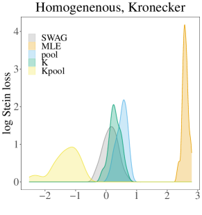
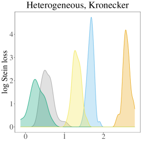
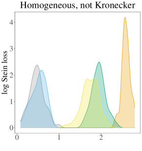
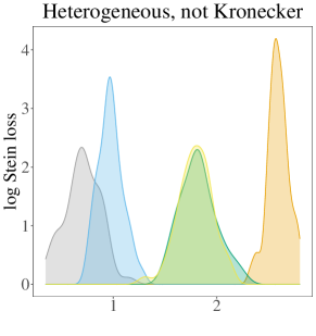
Figure 2: Empirical densities of the 50 $\log(\bar{L})$ values for each estimator given $J=4,p=12$.

Given population covariances homogeneous across population and not Kronecker structured, the pooled MLE and SWAG estimators have the two smallest average losses. In some cases considered, including the case where $J=4$ and $p=12$ in Figure 2, these two estimators perform similarly overall. All other estimators have comparatively large average loss. In particular, incorrectly assuming a Kronecker covariance in this regime results in estimators nearly as inaccurate as the sample covariances.

In the heterogeneous and Kronecker structured regime, the oracle estimator and the SWAG estimator have the two smallest average losses. Overall in this regime, these two estimators behave similarly and are notable improvements over the other estimators considered. This is particularly apparent in Figure 2 where the densities of the losses corresponding to $\hat{\boldsymbol{\Sigma}}$ and $\hat{\boldsymbol{K}}$ are smaller than and distinct from the densities corresponding to the other estimators considered.

In the fourth, and perhaps most realistic, regime considered, where population covariances are heterogeneous across population and not Kronecker structured, the SWAG estimator has the smallest average loss in cases with a small number of groups ($J=4$) and the second smallest average loss in cases with 10 groups. In this regime, the oracle estimator is outperformed by all other estimators considered. This is not surprising given the combination of the simplicity of the exchangeable population covariances in conjunction with large instability of the sample covariance due in part to the small sample sizes considered for each regime. Again, we see estimators based on an incorrect assumption of separability result in distinctly larger loss than the more flexible SWAG estimator (Figure 2).

Similar patterns are seen in the presence of only two populations (see Appendix B). Additionally, the posterior mean of the SWAG model, or the Bayes estimator under squared error loss, behaves similarly to the SWAG estimator in terms of accuracy. In total, these results support the conclusion that the SWAG model outperforms standard alternatives given the true structure of the population covariances is unknown. The flexibility of the SWAG model is particularly useful given the large error under estimators based on incorrect assumptions. In particular, wrongly assuming a Kronecker structure can result in an error nearly as large as that obtained under the sample covariance. While the extreme regimes considered do not necessarily reflect the truth in real-world scenarios, this simulation study highlights the flexibility of the SWAG model.

5 Examples

We demonstrate the usefulness of the SWAG model for estimating covariance matrices in multi-group matrix-variate populations by analyzing two data sets. In the first example, we perform a speech recognition task on a publicly available spoken-word audio dataset. In the second example, we analyze chemical exposure data which features small group-specific sample sizes.

5.1 Classification of spoken-word audio data

Classification of a new observation based on a labeled training dataset consisting of $n_{j}$ matrices, each with common dimensionality $p_{1}\times p_{2}$, observed from each of $j\in\{1,...,J\}$ populations is an important statistical task for speech recognition. To illustrate the utility of the SWAG covariance estimator, we analyze classification of spoken-audio samples of words “yes”, “no”, “up”, “down”, “left”, “right”, “on”, “off”,“stop”, and “go” from a dataset consisting of 1-second WAV files where each word has a sample size ranging from 1,987 to 2,103 (Warden, 2017, 2018). Audio data such as these are commonly described by mel-frequency cepstral coefficients (MFCCs) which represent the power spectrum of a sound across time increments. Accordingly, we represent each audio sample as a $p_{1}\times p_{2}$ feature matrix of the first $p_{1}=13$ MFCCs across $p_{2}=99$ time bins (Ligges et al., 2018).

One popular classification method for generic multivariate data is quadratic discriminant analysis (QDA). QDA is based on the result that, assuming normality and equal a priori probabilities of group membership, the probability of misclassification is minimized by assigning an unlabeled matrix $Y\in\mathbb{R}^{p_{1}\times p_{2}}$ to group $j\in\{1,...,J\}$ which minimizes the discriminant score function (Mardia et al., 1979),

$$D_{j}(Y)=(vec(Y)-\mu_{j})^{T}\Sigma_{j}^{-1}(vec(Y)-\mu_{j})+\log|\Sigma_{j}|,$$ (10)

where $\mu_{j}\in\mathbb{R}^{p}$ and $\Sigma_{j}\in\mathcal{S}^{+}_{p}$, $p=p_{1}p_{2}$, are respectively the mean vector and covariance matrix for population $j$ and $vec(\cdot)$ is the vectorization operator that stacks the columns of a matrix into a column vector. In practice, of course, these parameters are unknown and thus are estimated from a training data set. As a result, adequate performance of the classification relies on, among other things, accurate group-level covariance estimates.

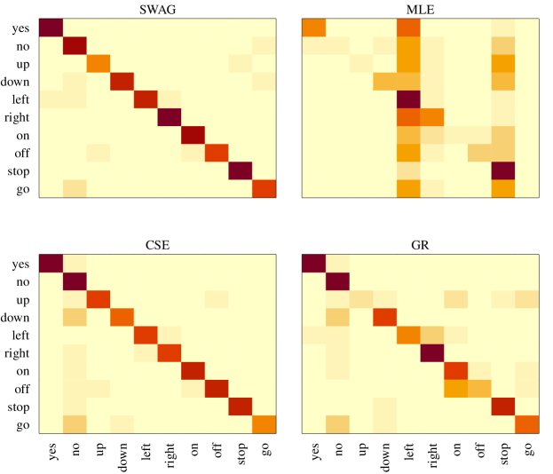
Figure 3: Confusion matrices resulting from classification from the various covariance estimates. Rows correspond to target words and columns correspond to predictions.

We display the utility of the multiple population SWAG estimators over standard estimators by comparing correct classification rates resulting from QDA in a leave-some-out comparison. To do this, we retain a random selection of $100$ observations from each population as a testing dataset, and the remaining observations constitute the training dataset. For the discriminant analysis, we use the sample mean to estimate each $\mu_{j}$ and a variety of covariance estimates for $\Sigma_{j}$, all computed from the training dataset. Specifically, we obtain the SWAG covariance estimates $\hat{\boldsymbol{\Sigma}}$ from output from the proposed Metropolis-Hastings algorithm run for 5,000 iterations with a burn-in of 200 and a thinning mechanism of 20. We compare this with the unstructured sample covariance obtained separately for each word $\boldsymbol{S}$, labeled MLE in this section. Additionally, we consider the partially pooled empirical Bayesian covariance estimate outlined in Greene and Rayens (1989) (GR), and the core shrinkage estimate (Hoff et al., 2022) which partially shrinks each word’s sample covariance matrix towards a separable covariance (CSE). Prior to computing the various covariance estimates, the data for each word is de-scaled and de-meaned. The scale is then re-introduced to the covariance estimates prior to conducting the classification analysis.

	SWAG	MLE	CSE	GR
yes	0.93	0.42	0.85	0.76
no	0.80	0.10	0.82	0.80
up	0.49	0.08	0.60	0.17
down	0.71	0.27	0.54	0.57
left	0.72	0.80	0.63	0.41
right	0.86	0.43	0.58	0.77
on	0.84	0.13	0.64	0.60
off	0.65	0.25	0.64	0.32
stop	0.87	0.80	0.70	0.63
go	0.66	0.05	0.47	0.47
average	0.75	0.33	0.65	0.55

Table 4: Rates of correct classification on audio test dataset from discriminant analysis under different covariance estimators. The average across all words for each method is displayed in the final row.

Classifications for the test observations are made using each covariance estimate, and results are summarized in confusion matrices displayed in Figure 3, with the true word classes along the rows and predicted word classes along the columns. The correct classification rates, or, the values of the diagonal elements in the confusion matrices, are contained in Table 4. In general, the SWAG classifier outperforms the other estimates. The SWAG estimate has a higher correct classification rate averaged over all words, and it features notably larger word-specific classification rates for the majority of words.

When comparing the SWAG estimate with the MLE, it features a significantly higher correct classification rate for every word except two, “left” and “stop”. Upon further inspection, however, the two large correct classification rates for the MLE are a feature of this classifier nearly always choosing one of these two words, as displayed in the confusion matrix. The correct classification rates obtained from the SWAG classifier are greater than or equal to those from the partially pooled estimate GR for every word, oftentimes by a large margin, which corresponds with a greater overall correct classification rate. Moreover, linear discriminant analysis, which uses a pooled covariance estimate $\hat{S}_{p}$ for each population covariance, performs even worse with an across-word average correct classification rate of 0.27. The most convincing competing classifier is the core shrinkage estimate. It has a larger correct classification rate for for the word “up” and correctly classifies two more observations for the word “no” than the SWAG estimate. While the CSE features slightly better performance for these two words, though, the SWAG classifier performs better over all populations. Furthermore, the SWAG classifier performs much better overall than the separable MLEs obtained separately for each population, $\hat{\boldsymbol{K}}$, which has an across-word average correct classification rate of 0.49. On the whole, the SWAG classifier outperforms the other classifiers considered with respect to accurate classification across all populations, and this example showcases the benefit of allowing for shrinkage both within and across populations.

5.2 Analysis of TESIE chemical exposures data

Many recent medical and environmental studies are concerned with understanding differences among socio-economic groups from repeated measurements of chemical exposures (James-Todd et al., 2017). In such an application, researchers may be interested in understanding within and across group heterogeneity. Additionally, researchers are often interested in understanding covariate effects and appropriately handling missing data. For all such tasks, accurate covariance modeling is critical.

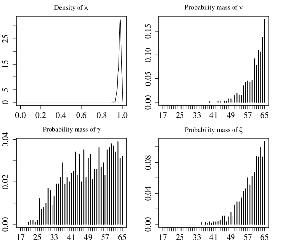
Figure 4: Approximations to the posterior distributions of key parameters $\lambda,\nu,\eta,$ and $\xi$ for the TESIE data example.

In this section, we analyze a sample gathered in the Toddlers Exposure to SVOCS in Indoor Environments (TESIE) study (Hoffman et al., 2018). In this study, biomarkers of various semi-volatile organic compounds (SVOCs) were extracted from paired samples of urine, blood, and silicone wristbands (see, e.g., Hammel et al. (2018)). In particular, each observation is a $p_{1}\times p_{2}$ matrix where the rows represent biomarkers from $p_{1}=5$ SVOCs obtained from the $p_{2}=3$ sources. Additionally, socio-economic covariates were collected for each individual in the study including highest education level attained and race, among others. We will analyze the $p_{1}p_{2}\times p_{1}p_{2}$ covariance matrices across education level as a proxy for different socio-economic populations. Specifically, the three education levels considered are less than high school (LHS), high school degree or GED (HS), and some college or college degree (C). The sample sizes are 30, 19, and 24 for the three populations defined by education levels LHS, HS, and C, respectively.

We proceed with estimating each population’s covariance with the SWAG model. While we remove the mean effect, the SWAG model can easily be extended to include a regression on covariates of interest. We run the Metropolis-Hastings sampler for 33,000 iterations, remove the first 3,000 iterations as a burn-in period, and retain every 30th sample as a thinning mechanism. Convergence is checked by examining trace plots.

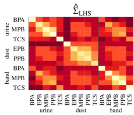
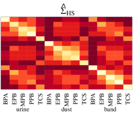
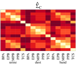
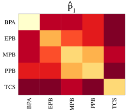
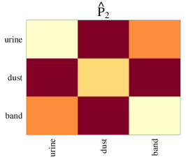
Figure 5: Bayes estimates under Stein’s loss of the covariances for the three populations LHS, HS, and C are plotted on the top row. Bayes estimates under Stein’s loss of the pooled Kronecker covariance are plotted on the bottom row.

Approximations to the posterior densities of shrinkage-controlling parameters $\lambda,\nu,\gamma,$ and $\xi$ are plotted in Figure 4. The posterior density of the weight on within versus across population shrinkage, $\lambda$, is concentrated around the upper bound of one, indicating that most of the weight is being placed on shrinking across groups towards a pooled covariance. Additionally, the posteriors of the degrees of freedom for across-group shrinkage $\nu$ and $\xi$ are concentrated around large values indicating strong shrinkage from an unstructured covariance towards a pooled Kronecker structured covariance. In this way, interpretation of summarizing across-row and across-column covariance estimates is straightforward.

This shrinkage behavior is evident upon comparing the Bayes estimates of the group-specific covariances $\hat{\Sigma}_{LHS},\hat{\Sigma}_{HS},$ and $\hat{\Sigma}_{C}$ to the Bayes estimates of the pooled Kronecker covariances $\hat{P}_{1}$ and $\hat{P}_{2}$ (Figure 5). Here, $\hat{P}_{1}$ is the across-SVOC covariance estimate and $\hat{P}_{2}$ is the across-source covariance estimate. The shrinkage towards a pooled separable structure is recognizable throughout the three group-specific covariance estimates. In particular, the general pattern of across-SVOC heterogeneity seen in $\hat{P}_{1}$ is roughly present in each 5x5 block in the group-specific covariances, seen in the top row of Figure 5. However, a benefit of the SWAG model is the ability to allow for divergences from this separable structure, a feature also discernible in the group-specific estimates. For example, within a given population, say, the LHS population, the pattern among the covariances between BPA and the other SVOCs from samples obtained from urine differs across measurement source by more than a single factor. Moreover, this pattern differs across populations which reflects heterogeneity across populations. In total, the output of the SWAG model allows for interpretation of a row covariance and a column covariance, shared across groups, while allowing for deviations from this structure at the group level.

6 Discussion

In this article, we propose a flexible model-based covariance estimation procedure for multi-group matrix-variate data. The SWAG hierarchical model provides a coherent approach to combining two common types of shrinkage, within populations towards a Kronecker structure and across populations towards a pooled covariance. Bayesian inference of model parameters is straightforward with a Metropolis-Hastings algorithm and allows for uncertainty quantification of covariance estimates. In simulation studies, we show the flexibility of the proposed method results in covariance estimates that outperform standard estimates in a wide array of settings in terms of loss.

The flexibility of the SWAG model is developed specifically for matrix-variate data, but the model and estimation procedure can be adapted for other types of data or applications. If the data being analyzed are not matrix-variate, different structures can be utilized in place of the Kronecker product. Additionally, the shrinkage towards a pooled covariance can be replaced to represent more complex relationships across the populations such as, for example, an autoregressive relationship. More simply, if population-specific flexibility is desired within the given framework, population-specific weights $\lambda_{1},..,\lambda_{J}$ can be introduced.

Replication codes are available at https://github.com/betsybersson/SWAG.

Appendix A Metropolis-Hastings Algorithm for SWAG

1. Sample $(\lambda,\boldsymbol{U})\sim p(w,\boldsymbol{U}|\boldsymbol{Y},\boldsymbol{\theta}_{-\lambda,-\boldsymbol{U}})$ as follows:

   1. sample $\lambda\sim p(\lambda|\boldsymbol{Y},\boldsymbol{\theta}_{-\boldsymbol{U},-\lambda})$ using a Metropolis step as follows:

      1. obtain a sample $\lambda^{*}$ from a symmetric random walk based on the previous iteration’s value of $\lambda$,

      2. compute the acceptance score

         $$r=\frac{p(\lambda^{*}|\boldsymbol{Y},\boldsymbol{\theta}_{-\boldsymbol{U},-\lambda})}{p(\lambda|\boldsymbol{Y},\boldsymbol{\theta}_{-\boldsymbol{U},-\lambda})},$$

      3. accept $\lambda^{*}$ as the new sample for $\lambda$ with probability $r$.

   2. sample $U_{j}|\boldsymbol{Y},\boldsymbol{\theta}_{-U_{j}}\sim N_{n_{j}\times p}\left(M_{j},S_{j}\,\otimes\,I_{n_{j}}\right)$ for each $j\in\{1,...,J\}$, where

      $$S_{j}={} \left(\Psi_{j}^{-1}+\frac{\lambda}{1-\lambda}\Lambda_{j}^{-1}\right)^{-1}$$

      $$M_{j}={} \frac{\lambda^{1/2}}{1-\lambda}Y_{j}\Lambda_{j}^{-1}S_{j}.$$

2. Sample $(\nu,\boldsymbol{\Psi})\sim p(\nu,\boldsymbol{\Psi}|\boldsymbol{Y},\boldsymbol{\theta}_{-\boldsymbol{\Psi},-\nu})$ as follows:

   1. sample $\nu$ where

      $$P\left(\nu=\nu^{*}|\boldsymbol{Y},\boldsymbol{\theta}_{-\boldsymbol{\Psi},-\nu}\right)=\frac{\prod_{j=1}^{J}p\left(U_{j}|\Psi_{0},\nu=\nu^{*}\right)}{\sum_{\nu^{{}^{\prime}}=p+2}^{p+k}\prod_{j=1}^{J}p\left(U_{j}|\Psi_{0},\nu=\nu^{{}^{\prime}}\right)},$$

      and $U_{j}|\Psi_{0},\nu\sim\text{T}_{n_{j}\times p}\left(\nu-p+1,0,\Psi_{0}(\nu-p-1)\,\otimes\,I_{n_{j}}\right)$,

   2. sample $\Psi_{j}|\boldsymbol{Y},\boldsymbol{\theta}_{-\Psi_{j}}\sim IW_{p}\big{(}\left(U_{j}^{T}U_{j}+(\nu-p-1)\Psi_{0}\right)^{-1},\nu+n_{j}\big{)}$ for each $j\in\{1,...,J\}$.

3. Sample $(\gamma,\boldsymbol{\Lambda})\sim p(\gamma,\boldsymbol{\Lambda}|\boldsymbol{Y},\boldsymbol{\theta}_{-\boldsymbol{\Lambda},-\gamma})$ as follows:

   1. sample $\gamma$ where

      $$P\left(\gamma=\gamma^{*}|\boldsymbol{Y},\boldsymbol{\theta}_{-\boldsymbol{\Lambda},-\gamma}\right)=\frac{\prod_{j=1}^{J}p\left(Y_{j}|\lambda,U_{j},R_{j},C_{j},\gamma=\gamma^{*}\right)}{\sum_{\gamma^{{}^{\prime}}=p+2}^{p+k}\prod_{j=1}^{J}p\left(Y_{j}|\lambda,U_{j},R_{j},C_{j},\gamma=\gamma^{{}^{\prime}}\right)},$$

      and $Y_{j}|\lambda,R_{j},C_{j}\sim T_{n_{j}\times p}\left(\gamma-p+1,\lambda^{1/2}U_{j},(1-\lambda)\left(C_{j}\,\otimes\,R_{j}\right)(\gamma-p-1)\,\otimes\,I_{n_{j}}\right)$,

   2. sample $\Lambda_{j}|\boldsymbol{Y},\boldsymbol{\theta}_{-\Lambda_{j}}\sim IW_{p}\big{(}\big{(}\tilde{Y}_{j}^{T}\tilde{Y}_{j}/(1-\lambda)+\left(C_{j}\,\otimes\,R_{j}\right)(\gamma-p-1)\big{)}^{-1},\gamma+n_{j}\big{)}$ in parallel for each $j\in\{1,...,J\}$ where $\tilde{Y}_{j}=\left(Y_{j}-w^{1/2}U_{j}\right)$.

4. Sample $\Psi_{0}|\boldsymbol{Y},\boldsymbol{\theta}_{-\Psi_{0}}\sim\text{W}_{p}\big{(}\big{(}(\nu-p-1)\sum_{j=1}^{J}\Psi_{j}^{-1}+\left(P_{2}\,\otimes\,P_{1}\right)^{-1}\xi\big{)}^{-1},\xi+J\nu\big{)}.$

5. Sample $R_{j}\sim\text{W}_{p_{1}}\big{(}\big{(}(\gamma-p-1)\sum_{k=1}^{p}L_{k}C_{j}L_{k}^{T}+R_{0}^{-1}\eta_{1}\big{)}^{-1},\eta_{1}+\gamma p_{2}\big{)}$ where $L_{k}=vec^{-1}(l_{k})$ from $\Lambda_{j}^{-1}=\tilde{L}\tilde{L}^{T}=\sum_{k=1}^{p}l_{k}l_{k}^{T}$, for each $j\in\{1,...,J\}$.

6. Sample $C_{j}\sim\text{W}_{p_{2}}\big{(}\left((\gamma-p-1)\sum_{k=1}^{p}L_{k}^{T}R_{j}L_{k}+C_{0}^{-1}\eta_{2}\right)^{-1},\eta_{2}+\gamma p_{1}\big{)}$ where $L_{k}=vec^{-1}(l_{k})$ from $\Lambda_{j}^{-1}=\tilde{L}\tilde{L}^{T}=\sum_{k=1}^{p}l_{k}l_{k}^{T}$, for each $j\in\{1,...,J\}$.

7. Sample $\xi$ where

   $$P\left(\xi=\xi^{*}|\boldsymbol{Y},\boldsymbol{\theta}_{-\xi}\right)=\frac{p\left(\Psi_{0}|P_{01},P_{02},\xi=\xi^{*}\right)}{\sum_{\xi^{{}^{\prime}}=p+2}^{p+k}p\left(\Psi_{0}|P_{01},P_{02},\xi=\xi^{{}^{\prime}}\right)}.$$

8. Sample $P_{1}\sim IW_{p_{1}}\big{(}\left(\xi\sum_{k=1}^{p}L_{k}P_{2}^{-1}L_{k}^{T}+P_{01}(\eta_{3}-p_{1}-1)\right)^{-1},\eta_{3}+\xi p_{2}\big{)}$ where $L_{k}=vec^{-1}(l_{k})$ from $\Psi_{0}^{-1}=\tilde{L}\tilde{L}^{T}=\sum_{k=1}^{p}l_{k}l_{k}^{T}$.

9. Sample $P_{2}\sim IW_{p_{2}}\big{(}\left(\xi\sum_{k=1}^{p}L_{k}^{T}P_{1}^{-1}L_{k}+P_{02}(\eta_{4}-p_{2}-1)\right)^{-1},\eta_{4}+\xi p_{1}\big{)}.$ where $L_{k}=vec^{-1}(l_{k})$ from $\Psi_{0}^{-1}=\tilde{L}\tilde{L}^{T}=\sum_{k=1}^{p}l_{k}l_{k}^{T}$.

Appendix B Simulation Study For Two Populations

	$\hat{\boldsymbol{\Sigma}}$	${\boldsymbol{S}}$	$\tilde{\boldsymbol{S}}$	$\hat{S}_{pool}$	$\hat{\boldsymbol{K}}$	$\hat{K}_{pool}$
Homogeneous, Kronecker

J = 2; p = 6	1.25	6.81	2.20	2.07	1.74	0.74
J = 2; p = 12	1.58	12.87	4.85	3.80	1.29	0.56
J = 2; p = 24	2.92	25.71	11.68	7.74	1.82	0.89

Homogeneous, not Kronecker
J = 2; p = 6	1.39	6.81	1.71	2.07	4.94	3.02
J = 2; p = 12	2.07	12.87	4.41	3.80	6.67	5.91
J = 2; p = 24	3.98	25.71	11.45	7.74	21.67	20.41

Heterogeneous, Kronecker
J = 2; p = 6	1.52	6.81	4.38	4.19	1.74	2.71
J = 2; p = 12	1.92	12.87	6.88	8.53	1.29	4.78
J = 2; p = 24	3.53	25.71	11.11	17.14	1.82	9.46

Heterogeneous, not Kronecker
J = 2; p = 6	1.45	6.81	1.70	2.20	5.60	3.68
J = 2; p = 12	2.31	12.87	4.24	4.04	7.75	7.19
J = 2; p = 24	4.11	25.71	10.95	8.33	26.34	24.80

Table 5: $\bar{L}$ values averaged over 50 iterations for $J=2$ populations and problem dimension $p=p_{1}p_{2}$. The oracle estimator for each regime has a grey background.

References

- Box (1949) Box, G. E. P. (1949). “A General Distribution Theory for a Class of Likelihood Criteria.” Biometrika, 36(3): 317–346.
- Brown et al. (1999) Brown, P. J., Fearn, T., and Haque, M. S. (1999). “Discrimination with many variables.” Journal of the American Statistical Association, 94(448): 1320–1329.
- Daniels (2006) Daniels, M. J. (2006). “Bayesian modeling of several covariance matrices and some results on propriety of the posterior for linear regression with correlated and/or heterogeneous errors.” Journal of Multivariate Analysis, 97: 1185–1207.
- Daniels and Kass (1999) Daniels, M. J. and Kass, R. E. (1999). “Nonconjugate Bayesian Estimation of Covariance Matrices and its Use in Hierarchical Models.” Journal of the American Statistical Association, 94(448): 1254–1263.
- Dawid (1981) Dawid, A. P. (1981). “Some matrix-variate distribution theory: notational considerations and a Bayesian application.” Biometrika, 68(1): 265–274.
- Flury (1987) Flury, B. K. (1987). “Two generalizations of the common principal component model.” Biometrika, 74(1): 59–69.
- Friedman et al. (2008) Friedman, J., Hastie, T., and Tibshirani, R. (2008). “Sparse inverse covariance estimation with the graphical lasso.” Biostatistics, 9(3): 432–441.
- Friedman (1989) Friedman, J. H. (1989). “Regularized discriminant analysis.” Journal of the American Statistical Association, 84(405): 165–175.
- Greene and Rayens (1989) Greene, T. and Rayens, W. S. (1989). “Partially pooled covariance matrix estimation in discriminant analysis.” Communications in Statistics - Theory and Methods, 18(10): 3679–3702.
- Hammel et al. (2018) Hammel, S. C., Phillips, A. L., Hoffman, K., and Stapleton, H. M. (2018). “Evaluating the Use of Silicone Wristbands To Measure Personal Exposure to Brominated Flame Retardants.” : Environ. Sci. Technol., 52: 11875–11885.
- Hoff et al. (2022) Hoff, P., Mccormack, A., and Zhang, A. R. (2022). “Core shrinkage covariance estimation for matrix-variate data.”
- Hoff (2009) Hoff, P. D. (2009). “A hierarchical eigenmodel for pooled covariance estimation.” Journal of the Royal Statistical Society: Series B (Statistical Methodology), 71(5): 971–992.
- Hoffman et al. (2018) Hoffman, K., Hammel, S. C., Phillips, A. L., Lorenzo, A. M., Chen, A., Calafat, A. M., Ye, X., Webster, T. F., and Stapleton, H. M. (2018). “Biomarkers of exposure to SVOCs in children and their demographic associations: The TESIE Study.” Environment International, 119(Cdc): 26–36.
- James-Todd et al. (2017) James-Todd, T. M., Meeker, J. D., Huang, T., Hauser, R., Seely, E. W., Ferguson, K. K., Rich-Edwards, J. W., and McElrath, T. F. (2017). “Racial and ethnic variations in phthalate metabolite concentration changes across full-term pregnancies.” Journal of Exposure Science and Environmental Epidemiology, 27(2): 160–160.
- Johnson et al. (2012) Johnson, B., Tateishi, R., and Xie, Z. (2012). “Using geographically weighted variables for image classification.” Remote Sensing Letters, 3(6): 491–499.
- Ligges et al. (2018) Ligges, U., Krey, S., Mersmann, O., and Schnackenberg, S. (2018). “tuneR: Analysis of Music and Speech.” Technical report.
- Lu and Zimmerman (2005) Lu, N. and Zimmerman, D. L. (2005). “The likelihood ratio test for a separable covariance matrix.” Statistics and Probability Letters, 73(4): 449–457.
- Mardia et al. (1979) Mardia, K., Kent, J., and Bibby, J. (1979). Multivariate Analysis. London: Academic Press, 1 edition.
- Marks and Dunn (1974) Marks, S. and Dunn, O. J. (1974). “Discriminant functions when covariance matrices are unequal.” Journal of the American Statistical Association, 69(346): 555–559.
- Rayens and Greene (1991) Rayens, W. and Greene, T. (1991). “Covariance pooling and stabilization for classification.” Computational Statistics and Data Analysis, 11(1): 17–42.
-
Warden (2017)
Warden, P. (2017).
“Speech commands: A public dataset for single-word speech
recognition.”
URL http://download.tensorflow.org/data/speech{_}commands{_}v0.01.tar.gz - Warden (2018) — (2018). “Speech commands: A dataset for limited-vocabulary speech recognition.” Technical report.
- Wu and Pourahmadi (2009) Wu, W. B. and Pourahmadi, M. (2009). “Banding sample autocovariance matrices of stationary processes.” Statistica Sinica, 19: 1755–1768.