On Frequency-Domain Implementation of Digital FIR Filters Using Overlap-Add and Overlap-Save Techniques

Abstract

In this paper, new insights in frequency-domain implementations of digital finite-length impulse response filtering (linear convolution) using overlap-add and overlap-save techniques are provided. It is shown that, in practical finite-wordlength implementations, the overall system corresponds to a time-varying system that can be represented in essentially two different ways. One way is to represent the system with a distortion function and aliasing functions, which in this paper is derived from multirate filter bank representations. The other way is to use a periodically time-varying impulse-response representation or, equivalently, a set of time-invariant impulse responses and the corresponding frequency responses. The paper provides systematic derivations and analyses of these representations along with filter impulse response properties and design examples. The representations are particularly useful when analyzing the effect of coefficient quantizations as well as the use of shorter DFT lengths than theoretically required. A comprehensive computational-complexity analysis is also provided, and accurate formulas for estimating the optimal DFT lengths for given filter lengths are derived. Using optimal DFT lengths, it is shown that the frequency-domain implementations have lower computational complexities (multiplication rates) than the corresponding time-domain implementations for filter lengths that are shorter than those reported earlier in the literature. In particular, for general (unsymmetric) filters, the frequency-domain implementations are shown to be more efficient for all filter lengths. This opens up for new considerations when comparing complexities of different filter implementations.

I Introduction

Digital finite-length impulse response (FIR) filtering (linear convolution) of an infinitely long (in practice very long) input sequence can be efficiently implemented in the frequency domain using overlap-add or overlap-save techniques [1, 2]. These techniques make use of the discrete Fourier transform (DFT) and its inverse (IDFT). In between the transforms, there is a diagonal matrix whose diagonal elements are the filter’s DFT coefficients, hereafter also referred to as DFT filter coefficients. The DFT and IDFT can be efficiently implemented using fast Fourier transform (FFT) algorithms which is the reason for the overall efficiency. The basic overlap-add and overlap-save principles are well known [1, 2], but there are few publications that consider their fundamental implementation properties. These techniques are however gaining an increasing interest, in particular in applications requiring long and/or many filters. Examples of such applications include equalization of chromatic dispersion in optical communications [3, 4, 5, 6, 7, 8], filter banks and channelizers with many channels [9, 10, 11, 12, 13], filters with narrow transition bands (don’t-care bands) [14], signal reconstruction/enhancement [15, 16], and predistortion in multiple-input multiple-output (MIMO) systems [17].

Most of the previous papers that utilize the overlap-save- or overlap-add-based implementations focus on the applications and study the overall system performance for different instances [5, 9, 10, 7, 8, 13, 17]. In this paper, the focus is instead on fundamental properties of the overlap-add and overlap-save implementations. For these implementations, as will be shown, the inevitable coefficient quantizations make the overall system a time-varying system instead of the intended time-invariant system. Hence, the analysis of coefficient quantization becomes more complicated than for the time-domain implementation, where it suffices to assess the frequency response of the filter with quantized coefficients [18, 19]. A time-varying system, on the other hand, cannot be characterized with a frequency response. Instead, such a system can be characterized in two different ways. One way is to represent it with a distortion function and aliasing functions which can be derived from a multirate filter bank (MFB) representation [20, 21], or via block digital filter representation which utilizes matrix-vector quantities [22, 23]. The other way is to use a periodically time-varying impulse-response (PTVIR) representation which corresponds to a set of time-invariant impulse responses and their respective frequency responses [20, 21].

The MFB and PTVIR representations make it possible to separate the coefficient quantization analysis from the data quantization analysis, which should be carried out separately [18, 19]. The representations are also useful when analyzing the effect of using shorter DFT lengths than theoretically required for a given impulse response length and input signal block length, which also results in a time-varying system. This occurs for example when designing the filter using its DFT coefficients as design parameters, and when the diagonal matrix between the DFT and IDFT is replaced with a more general matrix, both options used as a means to reduce the overall approximation error in the least-squares sense for given DFT and block lengths [22, 23]. In these generalized cases, the overall system is also referred to as a block digital filter [22]. Shorter DFT lengths also occur when using zero padding in the frequency domain as a means to carry out time-domain interpolation efficiently. An example of this will be presented in Section VI of this paper.

I-A Contributions

The main contributions of this paper are as follows.

• Systematic derivations and analyses of the MFB and PTVIR representations of the overlap-add and overlap-save frequency-domain implementations are provided. Analysis of frequency-domain implementation of linear convolution was also considered in [22, 23]. However, [22, 23] expressed the overall system in terms of the distortion and aliasing functions but did not explicitly express the overall system in terms of the MFB and PTVIR representations considered in this paper. Hence, this paper provides further insights for the design, analyses, and understanding, as it derives representations in terms of filters instead of matrix-vector quantities. It is noted here that some parts of this contribution have been presented at a conference [24], but only the basic principles of the overlap-add technique. Here, it is extended to incorporate the overlap-save technique and the additional contributions below.

• Expressions for the impulse responses in the PTVIR representation are derived and a detailed analysis of their lengths and relations is provided. This has not been considered earlier in the literature. The expressions hold for quantized coefficients as well, and are thus useful when analyzing the effects of coefficient quantization which, as mentioned before, should be carried out separately from the data quantization analysis [18, 19]. As will be shown, which is not obvious at first sight, the overlap-add and overlap-save techniques have different impulse response properties when using quantized coefficients (quantized DFT filter coefficients and complex exponentials in the DFT/IDFT), as well as shorter DFT lengths than theoretically required.

• A comprehensive computational-complexity analysis is provided, and the issue of selecting the optimal DFT length for a given filter length is addressed. Based on those results, we derive accurate formulas for estimating the optimal DFT lengths, which have not been reported before and differ from other works where optimal design refers to optimal overall filtering performance for fixed DFT and filter lengths [22, 23]. It will also be shown that, using optimal DFT lengths, that minimize the computational complexities (multiplication rates), the frequency-domain implementations become more efficient than the corresponding time-domain implementations for filter lengths that are shorter than those reported earlier in the literature [1, 25, 26]. In particular, for general (unsymmetric) filters, the frequency-domain implementations are shown to be more efficient for all filter lengths. This result opens up for new considerations when comparing complexities of different filter implementation options.

I-B Outline and Notations

Following this introduction, Section II recapitulates the overlap-add and overlap-save techniques. Sections III and IV derive the MFB and PTVIR representations, respectively. Section V analyzes the impulse response lengths and relations between the impulse responses in the PTVIR representation whereas Sections VI and VII provide design examples and computational-complexity analysis, respectively. Finally, Section VIII concludes the paper.

Throughout this paper, a sequence (discrete-time signal) is denoted as $x(n)$. The Fourier transform of $x(n)$ is defined by

$$X(e^{j\omega})=\sum_{n=-\infty}^{\infty}x(n)e^{-j\omega n},$$ (1)

with $\omega$ [rad] being the frequency variable (angle), and the inverse Fourier transform is given by

$$x(n)=\frac{1}{2\pi}\int_{-\pi}^{\pi}X(e^{j\omega})e^{j\omega n}d\omega.$$ (2)

The $z$-transform of $x(n)$, $X(z)$, is obtained from (1) by replacing $e^{j\omega}$ with the complex variable $z$. Further, the $N$-point DFT of a length-$N$ sequence $x(n),\,n=0,1,\ldots,N-1$, is defined by

$$X(k)=\sum_{n=0}^{N-1}x(n)e^{-j2\pi kn/N},\quad k=0,1,\ldots,N-1,$$ (3)

whereas the IDFT is given by

$$x(n)=\frac{1}{N}\sum_{k=0}^{N-1}X(k)e^{j2\pi kn/N},\quad n=0,1,\ldots,N-1.$$ (4)

We refer to $X(k)$ as the DFT coefficients of $x(n)$. For an impulse response $h(n)$ of a filter, we refer to $H(k)$ as the DFT filter coefficients.

II Overlap-Add and Overlap-Save Techniques

The point of departure is that we are to implement a digital FIR filter with the impulse response $h(n)$ of length $L$ (and thus having a filter order of $L-1$), for an input sequence $x(n)$ generating an output sequence $y(n)$. This corresponds to linear convolution according to

$$y(n)=\sum_{p=0}^{L-1}h(p)x(n-p).$$ (5)

For convenience in the equations that follow, we have here assumed that the input $x(n)$ is zero for negative values of $n$. The linear convolution can be implemented in the frequency domain using the overlap-add and overlap-save methods as detailed below. Both methods utilize a zero-padded impulse response sequence of length

$$N=L+M-1,$$ (6)

according to

$$h_{z}(n)=\begin{cases}h(n),&n=0,1,\ldots,L-1,\\ 0,&n=L,L+1,\ldots,N-1.\end{cases}$$ (7)

In the implementation, the $N$ DFT filter coefficients of $h_{z}(n)$, say $H(k),\,k=0,1,\ldots,N-1$, will be used. They are given by

$$H(k)=\sum_{n=0}^{N-1}h_{z}(n)e^{-j2\pi nk/N}=\sum_{n=0}^{L-1}h(n)e^{-j2\pi nk/N}.$$ (8)

Further, $M$ denotes the length of the input segments (output segments) in the overlap-add (overlap-save) methods.

II-A Overlap-Add Method

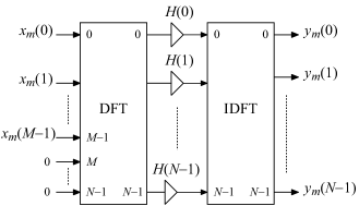
Figure 1: Frequency-domain computation of the output segment $y_{m}(n)$ in the overlap-add technique.

In the overlap-add method [2], the input sequence $x(n)$ is divided into adjacent input segments $x_{m}(n),\,m=0,1,2,\ldots,$ of length $M$. Then, each input segment is zero-padded to form a sequence of length $N=L+M-1$ according to

$$x_{m}(n)=\begin{cases}x(n+mM),&n=0,1,\ldots,M-1,\\ 0,&n=M,M+1,\ldots,N-1.\end{cases}$$ (9)

Also utilizing the zero-padded length-$N$ impulse response sequence $h_{z}(n)$ in (7), the output $y(n)$ can then be computed as a sum of shifted and partially overlapping output segments of length $N$ according to

$$y(n)=\sum_{m=0}^{\infty}y_{k}(n-mM),$$ (10)

where the output segments $y_{m}(n)$ are obtained from the convolution

$$y_{m}(n)=\sum_{p=0}^{N-1}h_{z}(p)x_{m}(n-p)=\sum_{p=0}^{L-1}h(p)x_{m}(n-p).$$ (11)

Each output segment $y_{m}(n)$ can be computed by pointwise multiplying $H(k)$ by $X_{m}(k)$, i.e., the length-$N$ DFT coefficients of $x_{m}(n)$, and computing the length-$N$ IDFT of the so obtained result. This is depicted in Fig. 1. Since the length of the output segments $y_{k}(n)$ is $N$, whereas each of these segments is shifted $mM$ samples to form the output $y(n)$, there is an overlap of $L-1$ samples between consecutive output segments. For the overlapping time indices, the samples of the corresponding output segments are consequently added to form the output samples. For the remaining time indices, the output samples are taken directly from the corresponding output segment. Utilizing upsamplers and downsamplers [20], the overlap-add method can be represented by the structure in Fig. 2.

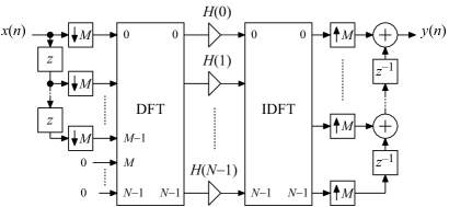
Figure 2: Frequency-domain implementation using the overlap-add technique.

II-B Overlap-Save Method

In the overlap-save method [2], the input sequence $x(n)$ is divided into overlapping input segments $x_{m}(n),\,m=0,1,2,\ldots,$ of length $N$ according to

$$x_{m}(n)=x(n+mM),\,n=0,1,\ldots,N-1.$$ (12)

The output $y(n)$ can again be computed as a sum of output segments $y_{m}(n)$ according to (10). However, here, $y_{m}(n)$ are length-$M$ segments and thus adjacent, not overlapping. They are obtained as

$$y_{m}(n)=y_{mC}(n+L-1),\,n=0,1,\ldots,M-1,$$ (13)

where each $y_{mC}(n)$ is the length-$N$ output of the circular convolution between $h_{z}(p)$ and $x_{m}(n)$, as given by [2]

$$y_{mC}(n)=\sum_{p=0}^{N-1}h_{z}(p)x_{m}(n-p\textnormal{ mod }N).$$ (14)

Each output segment $y_{m}(n)$ can be computed by first pointwise multiplying $H(k)$ by $X_{m}(k)$, then computing the length-$N$ IDFT of the so obtained result, and finally discarding the first $L-1$ values of the $N$ IDFT output values. This is illustrated in Fig. 3. An advantage of the overlap-save technique is that the output segments do not overlap which means that the output additions present in the overlap-add method are avoided. However, there are also other implementation aspects to consider, which means that the overlap-add technique may still be competitive as to the overall implementation complexity. In particular, one needs to consider the fact that the overlap-add technique uses a DFT with $L-1$ inputs being zero, whereas the overlap-save technique uses an IDFT with $L-1$ outputs being unused. Hence, in both cases, some operations in the DFT and IDFT may be removed. The exact amount of savings depend on the architecture as well as the values of $L$, $M$, and $N$.

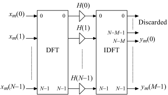
Figure 3: Frequency-domain computation of the output segment $y_{m}(n)$ in the overlap-save technique.

Finally, again utilizing upsamplers and downsamplers [20], the overlap-save method can be represented by the structure in Fig. 4 where $H(k)$, $k=0,1,\ldots,N-1$, are again the $N$ DFT coefficients of $h_{z}(n)$ given by (8).

III Multirate Filter Bank Representation

Using properties of DFT FBs [20], the scheme in Fig. 2 can be equivalently represented by an $N$-channel MFB, as depicted in Fig. 5, with analysis filters $G_{k}(z)$, $k=0,1,\ldots,N-1$, and synthesis filters $F_{k}(z)$, $k=0,1,\ldots,N-1$, as described below for the two cases. It is stressed that the MFB representation in Fig. 5 is used for analysis purposes only. It should not be used for the implementation of the overlap-add and overlap-save techniques, as its complexity is higher than the complexities of the schemes in Figs. 2 and 4.

III-A Overlap-Add

In this case, the analysis and synthesis filters have length-$M$ and length-$N$ impulse responses, respectively, and are given by

$$g_{k}(n)=e^{j2\pi(n-M+1)k/N},\quad n=0,1,\ldots,M-1,$$ (15)

and

$$f_{k}(n)=\frac{1}{N}e^{j2\pi nk/N},\quad n=0,1,\ldots N-1.$$ (16)

The corresponding frequency responses are

$$G_{k}(e^{j\omega})=\sum_{n=0}^{M-1}e^{j2\pi(n-M+1)k/N}e^{-j\omega n}$$ (17)

and

$$F_{k}(e^{j\omega})=\frac{1}{N}\sum_{n=0}^{N-1}e^{j2\pi nk/N}e^{-j\omega n}.$$ (18)

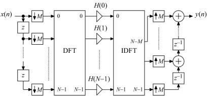
Figure 4: Frequency-domain implementation using the overlap-save technique.

Figure 5: MFB representation of the schemes in Figs. 2 and 4. It is used for analysis purposes only.

III-B Overlap-Save

Here, the analysis and synthesis filters have length-$N$ and length-$M$ impulse responses, respectively, and are given by

$$g_{k}(n)=e^{j2\pi(n+1)k/N},\quad n=0,1,\ldots,N-1,$$ (19)

and

$$f_{k}(n)=\frac{1}{N}e^{j2\pi(n-M)k/N},\quad n=0,1,\ldots,M-1.$$ (20)

The corresponding frequency responses are

$$G_{k}(e^{j\omega})=\sum_{n=0}^{N-1}e^{j2\pi(n+1)k/N}e^{-j\omega n}$$ (21)

and

$$F_{k}(e^{j\omega})=\frac{1}{N}\sum_{n=0}^{M-1}e^{j2\pi(n-M)k/N}e^{-j\omega n}.$$ (22)

III-C Distortion and Aliasing Functions

Based on the MFB representation in Fig. 5, one can express the output Fourier transform $Y(e^{j\omega})$ as

$$Y(e^{j\omega})=\sum_{p=0}^{M-1}V_{p}(e^{j\omega})X\big{(}e^{j(\omega-2\pi p/M)}\big{)},$$ (23)

where $V_{0}(e^{j\omega})$ is the distortion frequency response whereas the remaining $V_{p}(e^{j\omega})$, $p=1,2,\ldots,M-1$, are aliasing frequency responses. Using well-known input-output relations of MFBs [20], it follows that $V_{p}(e^{j\omega})$ are given by

$$V_{p}(e^{j\omega})=\frac{1}{M}\sum_{k=0}^{N-1}H(k)G_{k}\big{(}e^{j(\omega-2\pi p/M)}\big{)}F_{k}(e^{j\omega})$$ (24)

where $H(k)$ is given by (8) whereas $G_{k}(e^{j\omega})$ and $F_{k}(e^{j\omega})$ are the frequency responses of $g_{k}(n)$ and $f_{k}(n)$, as given by (17) and (18) for overlap-add and by (21) and (22) for overlap-save.

Using infinite-precision DFT and IDFT coefficients, we have $V_{0}(e^{j\omega})=H(e^{j\omega})$, where $H(e^{j\omega})$ is the frequency response of $h(n)$, i.e.,

$$H(e^{j\omega})=\sum_{n=0}^{L-1}h(n)e^{-j\omega n},$$ (25)

whereas all aliasing terms are zero, i.e., $V_{p}(e^{j\omega})=0$ for $p=1,2,\ldots,M-1$. However, when the DFT coefficients and complex exponentials in the DFT/IDFT are quantized (see Footnote 1), aliasing will be introduced. This means that the frequency-domain implementation of linear convolution corresponds to a weakly time-varying system instead of the desired time-invariant system. The above representation is a useful tool for analyzing the overall system performance when quantizing the coefficients. One can thereby set requirements on $V_{0}(e^{j\omega})$ to approximate $H(e^{j\omega})$ and on $V_{p}(e^{j\omega})$, $p=1,2,\ldots,M-1$, to approximate zero. Alternatively, depending on the application, it may be better to use a PTVIR representation to assess the overall performance.

IV Periodically Time-Varying Impulse-Response Representation

An MFB with $M$-fold downsampling and upsampling, as in Fig. 5, corresponds to an $M$-periodic linear system [21, 27]. The output $y(n)$ of such a system, assuming an FIR system with impulse response lengths $L_{n}$, is given by

$$y(n)=\sum_{q=0}^{L_{n}-1}h_{n}(q)x(n-q),$$ (26)

where $h_{n}(q)=h_{n+M}(q)$ denotes the $M$-periodic impulse response of the system. Due to the periodicity, such a system is completely characterized by a set of $M$ impulse responses, $h_{n}(q)$, $n=0,1,\ldots,M-1$, and thus by the $M$ corresponding frequency responses

$$H_{n}(e^{j\omega})=\sum_{q=0}^{L_{n}-1}h_{n}(q)e^{-j\omega q}.$$ (27)

Using the inverse Fourier transform, the output can then alternatively be written as

$$y(n)=\frac{1}{2\pi}\int_{-\pi}^{\pi}H_{n}(e^{j\omega})X(e^{j\omega})e^{j\omega n}d\omega.$$ (28)

From the filtering point of view, this means that different output samples are affected by different frequency responses, $H_{n}(e^{j\omega})$. When $H_{n}(e^{j\omega})=H(e^{j\omega})$ for all $n$, the system reduces to a regular linear and time-invariant filter with the frequency response $H(e^{j\omega})$. In the frequency-domain implementation of linear convolution, this is the desired result and corresponds to $V_{0}(e^{j\omega})=H(e^{j\omega})$ and $V_{p}(e^{j\omega})=0$, $p=1,2,\ldots,M-1$, in the MFB representation. Using the PTVIR representation, the overall system performance is thus evaluated by studying $H_{n}(e^{j\omega})$, all of which should approximate $H(e^{j\omega})$.

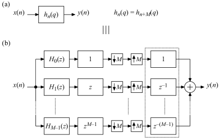
Figure 6: PTVIR representations of the schemes in Figs. 2 and 4.

The $M$ frequency responses $H_{n}(e^{j\omega})$ can be derived from the analysis and synthesis filters in Fig. 5. To this end, it is first observed that the $M$-periodic impulse response representation, depicted in Fig. 6(a), can be equivalently represented by the structure in Fig. 6(b) [27]. This structure can also be viewed as an MFB representation, with trivial synthesis filters, but it should not be confused with the general MFB representation in Fig. 5 of Section III. Hence, regardless of whether the representation in Fig. 6(a) or (b) is used, we still refer to it as the PTVIR representation. Using polyphase decomposition, and properties of downsamplers and upsamplers [20], it follows that the transfer functions $H_{n}(z)$ can be expressed as

$$H_{n}(z)=z^{-n}\sum_{k=0}^{N-1}H(k)G_{k}(z)F_{kn}\big{(}z^{M}\big{)},$$ (29)

where $F_{kn}(z)$ denote the polyphase components of $F_{k}(z)$ in the $M$-fold polyphase decomposition

$$F_{k}(z)=\sum_{n=0}^{M-1}z^{-n}F_{kn}\big{(}z^{M}\big{)}.$$ (30)

Table I: Properties of the Impulse Responses $h_{n}(q),\,n=0,1,\ldots,M-1$, for the Overlap-Add and Overlap-Save Methods.

Property	Effective length	Impulse responses	Impulse responses
		with quantized $H(k)$	with quantized $f_{k}(n)$ and/or $g_{k}(n)$
Overlap-add, $N\neq KM$	$M\times\left\lfloor(N-1-n)/M\right\rfloor+M$	Not circularly shifted	Not circularly shifted
Overlap-add, $N=KM$	$N$	Circularly shifted	Not circularly shifted
Overlap-save, all $N$	$N$	Circularly shifted	Not circularly shifted

Conversely, we can also express the distortion and aliasing functions of the MFB representation in terms of $H_{n}(z)$. Using again well-known input-output relations of MFBs [20], it follows that $V_{p}(e^{j\omega})$ can be expressed as

$$V_{p}(e^{j\omega})=\frac{1}{M}\sum_{n=0}^{M-1}H_{n}\big{(}e^{j(\omega-2\pi p/M)}\big{)}e^{-j2\pi pn/M}.$$ (31)

It is seen that the distortion frequency response $V_{0}(e^{j\omega})$ is the average of the $M$ filter frequency responses $H_{n}(e^{j\omega})$, whereas each aliasing frequency response $V_{p}(e^{j\omega})$, $p=1,2,\ldots,M-1,$ is the average of frequency-shifted and rotated (due to the multiplication by $e^{-j2\pi pn/M}$) versions of $H_{n}(e^{j\omega})$. This means that a metric based on $H_{n}(e^{j\omega})$ instead of $V_{p}(e^{j\omega})$ may be a better indicator of the worst-case time-domain error of the overall system. This will be exemplified in Section VI.

V Impulse Response Properties

Using finite-wordlength coefficients, i.e., quantized DFT filter coefficients $H(k)$ and/or quantized complex exponentials in the DFT/IDFT, i.e., quantized $g_{k}(n)$ and/or $f_{k}(n)$ (see Footnote 1), the overlap-add and overlap-save methods have different properties regarding the lengths of and relations between the $M$ impulse responses $h_{n}(q),\,n=0,1,\ldots,M-1$. The properties are summarized in Table I. They can be deduced from (29) which will be shown and discussed in detail below in subsections V-A and V-B. For convenience, both filter length and order will be used in those sections, recalling that the length is the order plus one. Further, the effective order (and length) will be considered. For an FIR filter with non-zero impulse response values $h(n)$ for $n=n_{1},n_{1}+1,\ldots,n_{2}$, the effective order is $n_{2}-n_{1}$, and thus the effective length is $n_{2}-n_{1}+1$.

V-A Overlap-Add

For the overlap-add method, the length of $g_{k}(n)$ is $M$ whereas the length of $f_{k}(n)$ is $N$. It is seen in (29) that $H_{n}(z)$ depends on $G_{k}(z)$ and the polyphase components of $F_{k}(z)$, i.e., $F_{kn}(z^{M})$ as given by (30). This means that the effective filter order, say $K_{n}$, of $H_{n}(z)$ is $K_{n}=M-1+K_{F_{n}}M$ which corresponds to the order of $H(k)G_{k}(z)F_{kn}(z^{M})$, where $M-1$ is the order of all $G_{k}(z)$ whereas $K_{F_{n}}$ denote the orders of $F_{kn}(z)$. The highest-power term in (29) is however $K_{n}+n$ due to the multiplication of $z^{-n}$. Thus, in the time domain, each impulse response $h_{n}(q)$ is obtained through an $n$-step right-shift of the impulse response of $H(k)G_{k}(z)F_{kn}(z^{M})$. It will thus have $n-1$ initial zero-valued impulse response values. Furthermore, the effective order $K_{n}$ depends on $n$ in general. This is because $K_{F_{n}}$ are generally not the same for all $n$. The exception is when $N$ is an integer multiple of $M$, say $N=KM$, in which case $K_{F_{n}}=K-1$ for all $n$ and, consequently, $K_{n}=M-1+(K-1)M=N-1$ for all $n$. In general, when $N\neq KM$, $K_{F_{n}}=\left\lfloor(N-1-n)/M\right\rfloor$.

Further, since the order of $G_{k}(z)$ is $M-1$, and $G_{k}(z)$ is multiplied by $F_{kn}(z^{M})$ when expressing the overall transfer function $H_{n}(z)$ in (29), the impulse response of $z^{n}H_{n}(z)$, say $d_{n}(q)$, only depends on $g_{k}(m)$ for one distinct time index $m$ for each $q$. To be precise, it follows from (15), (16), and (29) that $d_{n}(q)$, $q=0,1,\ldots,K_{n}$, can be expressed as

$$d_{n}(q)=\sum_{k=0}^{N-1}H(k)\sum_{r=0}^{K_{F_{n}}}g_{k}(q-rM)f_{k}(n+rM).$$ (32)

Since the length of $g_{k}(q)$ is $M$, $g_{k}(q-rM)$ correspond to nonoverlapping right-shifted (by $M$) versions of $g_{k}(q)$. Hence, for each $q$, only one term in the right-most sum in (32) is non-zero.

For the special case when $N=KM$, and thus $K_{F_{n}}=K-1$, $d_{n}(q)$ can be written as

$$d_{n}(q) = \sum_{k=0}^{N-1}H(k)\sum_{r=0}^{K-1}g_{k}(q-rM)f_{k}(n+rM)$$ (33)

$$= \frac{1}{N}\sum_{k=0}^{N-1}H(k)$$

$$\times \sum_{r=0}^{K-1}e^{j2\pi(q-M+1-rM)k/N}e^{j2\pi(n+rM)k/N}$$

$$= \frac{1}{N}\sum_{k=0}^{N-1}H(k)e^{j2\pi(q-M+1+n)k/N}.$$

The last equality holds since only one term in the $K$-term summation is non-zero for each $q$. When $H(k)$ are quantized, but $g_{k}(q)$ and $f_{k}(q)$ are not quantized, $d_{n}(q)$ are circularly shifted [2] versions of each other, which means that all $M$ impulse responses contain the same set of $N$ values. To show this, consider $d_{n+m}(q)$ which amounts to replacing $n$ with $n+m$ in (33). As seen in (33), this is equivalent to replacing $q$ with $q+m$, which corresponds to $d_{n}(q)$ circularly shifted to the left by $m$ samples. It is also noted that $-M+1$ on the last two lines of (33) emanates from the additional delay of $M-1$ samples due to the block processing, as mentioned in Footnote 5.

In the general case, when $N\neq KM$, $K_{F_{n}}$are not the same for all $n$, in which case (32) is still valid, but not (33). Here, since all $d_{n}(q)$ do not have the same length, the circular-shift property is lost. The property is also lost for all $N$ when $g_{k}(q)$ and $f_{k}(q)$ are quantized, meaning that the complex exponentials in (33) are quantized (see Footnote 1). This is because the two independently quantized exponentials, on the second last line in (33), will have index-dependent quantization errors and the last equality and equivalence utilized above will then no longer hold.

Table II: Example 1: Original Impulse Response $h(q)$ (Right-Shifted) and Overlap-Add Impulse Responses $h_{n}(q),\,n=0,1,2,3$, Using Quantized $H(k)$ but Unquantized $g_{k}(n)$ and $f_{k}(n)$, Illustrating That the Circular-Shift Property Does Not Hold When $N\neq KM$.

Original, $h(q-3)$	$h_{0}(q)$	$h_{1}(q)$	$h_{2}(q)$	$h_{3}(q)$
0	0.000815299395028	0	0	0
0	0.000030422174521	0.000030422174521	0	0
0	0.000083095006610	0.000083095006610	0.000083095006610	0
-0.065517977199101	-0.064843750000000	-0.064843750000000	-0.064843750000000	-0.064843750000000
0.054777425047761	0.054418477371339	0.054418477371339	0.054418477371339	0.054418477371339
0.314937451772624	0.314709622812781	0.314709622812781	0.314709622812781	0.314709622812781
0.464142316077418	0.464214378227023	0.464214378227023	0.464214378227023	0.464214378227023
0.314937451772624	0.315733563910444	0.315733563910444	0.315733563910444	0.315733563910444
0.054777425047761	0.054687500000000	0.054687500000000	0.054687500000000	0.054687500000000
-0.065517977199101	-0.065629858897746	-0.065629858897746	-0.065629858897746	-0.065629858897746
0	0.000815299395028	0.000815299395028	0	0.000815299395028
0	0.000030422174521	0.000030422174521	0	0
0	0	0.000083095006611	0	0

Table III: Example 1: Original Impulse Response $h(q)$ (Right-Shifted) and Overlap-Save Impulse Responses $h_{n}(q),\,n=0,1,2,3$, Using Quantized $H(k)$ but Unquantized $g_{k}(n)$ and $f_{k}(n)$, Showing the Circular-Shift Property.

Original, $h(q-3)$	$h_{0}(q)$	$h_{1}(q)$	$h_{2}(q)$	$h_{3}(q)$
0	0.000815299395028	0	0	0
0	0.000030422174521	0.000030422174521	0	0
0	0.000083095006610	0.000083095006610	0.000083095006610	0
-0.065517977199101	-0.064843750000000	-0.064843750000000	-0.064843750000000	-0.064843750000000
0.054777425047761	0.054418477371339	0.054418477371339	0.054418477371339	0.054418477371339
0.314937451772624	0.314709622812781	0.314709622812781	0.314709622812781	0.314709622812781
0.464142316077418	0.464214378227023	0.464214378227023	0.464214378227023	0.464214378227023
0.314937451772624	0.315733563910444	0.315733563910444	0.315733563910444	0.315733563910444
0.054777425047761	0.054687500000000	0.054687500000000	0.054687500000000	0.054687500000000
-0.065517977199101	-0.065629858897746	-0.065629858897746	-0.065629858897746	-0.065629858897746
0	0	0.000815299395028	0.000815299395028	0.000815299395028
0	0	0	0.000030422174521	0.000030422174521
0	0	0	0	0.000083095006610

Table IV: Example 1: Original Impulse Response $h(q)$ (Right-Shifted) and Overlap-Save Impulse Responses $h_{n}(q),\,n=0,1,2,3$, Using Quantized $H(k)$, $g_{k}(n)$, and $f_{k}(n)$, Showing That the Circular-Shift Property Is Lost.

Original, $h(q-3)$	$h_{0}(q)$	$h_{1}(q)$	$h_{2}(q)$	$h_{3}(q)$
0	0.001343357563019	0	0	0
0	0.000361371040344	0.000361371040344	0	0
0	0.000538158416748	0.000160551071167	0.000538158416748	0
-0.065517977199101	-0.064286172389984	-0.064312195777893	-0.064312195777893	-0.064286172389984
0.054777425047761	0.054309082031250	0.054947161674500	0.054378080368042	0.054947161674499
0.314937451772624	0.313703811168671	0.314443969726562	0.314058876037598	0.314058876037598
0.464142316077418	0.463059282302857	0.463059282302857	0.463626098632813	0.463081991672516
0.314937451772624	0.315321087837219	0.314716339111328	0.315321087837219	0.315228271484375
0.054777425047761	0.054968869686127	0.054803586006165	0.054803586006165	0.054968869686127
-0.065517977199101	-0.065100097656250	-0.065209484100342	-0.065339374542236	-0.065209484100342
0	0	0.001248168945313	0.000872826576233	0.000872826576233
0	0	0	0.000271606445313	0.000208508968353
0	0	0	0	0.000347900390625

V-B Overlap-Save

Here, the order of $F_{k}(z)$ is $M-1$, which means that the order of all polyphase components $F_{kn}(z^{M})$ is zero, whereas the order of $G_{k}(z)$ is $N-1$. Consequently, the effective order is $K_{n}=N-1$ for all $n$. This coincides with the special case of the overlap-add method with $N=KM$.

Further, when $H(k)$ are quantized, but $g_{k}(q)$ and $f_{k}(q)$ are unquantized, the impulse responses of $z^{n}H_{n}(z)$, $d_{n}(q)$, are circularly shifted versions of each other regardless of the values of $N$ and $M$. This is different from the overlap-add method for which this property holds only when $N=KM$. For the overlap-save method, it holds for all $N$ and $M$ because the order of all polyphase components $F_{kn}(z^{M})$ is zero. Consequently, each $F_{kn}(z^{M})$ is here a constant, viz. $F_{kn}(z^{M})=f_{k}(n)$, and it then follows from (19), (20), and (29), that $d_{n}(q)$ can be written as

$$d_{n}(q) = \sum_{k=0}^{N-1}H(k)g_{k}(q)f_{k}(n)$$ (34)

$$= \frac{1}{N}\sum_{k=0}^{N-1}H(k)e^{j2\pi(q+1)k/N}e^{j2\pi(n-M)k/N}$$

$$= \frac{1}{N}\sum_{k=0}^{N-1}H(k)e^{j2\pi(q+1+n-M)k/N}.$$

Consider now $d_{n+m}(q)$ which amounts to replacing $n$ with $n+m$ in (34). As seen in (34), this is equivalent to replacing $q$ with $q+m$, which corresponds to $d_{n}(q)$ circularly shifted to the left by $m$ samples. As for the overlap-add method, the property is however lost when $g_{k}(q)$ and $f_{k}(q)$ are quantized.

VI Design Examples

Example 1. This example will illustrate the impulse response properties provided in Section V. To this end, we use a linear-phase FIR filter of length $L=7$, a block length of $M=4$ and a DFT length of $N=10$. We have used an equiripple design, assuming passband and stopband edges at $0.3\pi$ and $0.6\pi$, respectively, and equal passband and stopband ripples. When rounding, we have used $8$ fractional bits.

Table II gives the original impulse response $h(q)$ (right-shifted three steps to ease the comparison) and the four impulse responses $h_{n}(q),\,n=0,1,2,3$, when using the overlap-add method and with $H(k)$ quantized. It is seen that the impulse responses have different effective lengths and that the circular-shift property does not hold which is because $N\neq KM$. Table III gives the corresponding impulse responses for the overlap-save method. Here, it is seen that the impulse responses have the same effective length and that the circular-shift property holds. However, as seen in Table IV, when $g_{k}(n)$ and $f_{k}(n)$ are quantized as well (i.e., the complex exponentials in the DFT/IDFT are quantized, see Footnote 1), also the overlap-save method loses the circular-shift property, but the impulse responses are still of the same effective length.

Example 2: This example will illustrate the frequency-domain properties of the MFB and PTVIR representations. To this end, we first design an equiripple linear-phase FIR filter of length $L=35$ and with passband and stopband edges at $0.3\pi$ and $0.5\pi$, respectively, and passband and stopband ripples of $0.001$ ($-60$ dB). The frequency response $H(e^{j\omega})$ of the initial filter with infinite precision (here Matlab precision) impulse response values (coefficients) $h$($n$) is seen in Fig. 7. Next, we implement the filter with the overlap-add method (Fig. 2) with $M=30$, and thus $N=64$, and with eight fractional bits for $H(k)$ as well as for $g_{k}(n)$ and $f_{k}(n)$. The resulting distortion and aliasing frequency responses $V_{0}(e^{j\omega})$ and $V_{p}(e^{j\omega})$, $p=1,2,\ldots,M-1$, in the MFB representation (Fig. 5) are seen in Figs. 8 and 9, respectively. The corresponding frequency responses $H_{n}(e^{j\omega})$ in the PTVIR representation (Fig. 6) are plotted in Fig. 10. As seen, the worst-case responses of $H_{n}(e^{j\omega})$ are some $10$ dB larger than the aliasing terms in the stopband. This illustrates that, in applications where the worst-case time-domain error (difference between the actual output $y(n)$ and the desired one) is more important than the average error, a metric based on $H_{n}(e^{j\omega})$ instead of $V_{p}(e^{j\omega})$ is more appropriate.

To further illustrate the difference between the MFB and PTVIR representations, we perform the same analysis as above, but here with a reduced DFT length of $N=56$ instead of quantized coefficients. The corresponding frequency responses are plotted in Figs. 11–13. It is seen that the difference between the two representations is more pronounced in this case as the difference between the best and worst $H_{n}(e^{j\omega})$ is quite large. It also illustrates that one can only use slightly shorter DFT lengths than theoretically required. Otherwise, the performance degradation becomes very large.

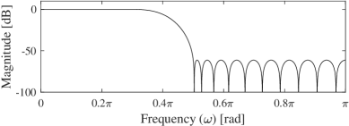
Figure 7: Examples 2: Initial infinite-precision filter frequency response $H(e^{j\omega})$.

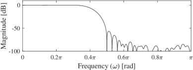
Figure 8: Example 2: Distortion frequency response $V_{0}(e^{j\omega})$.

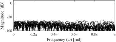
Figure 9: Example 2: Aliasing frequency responses $V_{p}(e^{j\omega})$, $p=1,2,\ldots,M-1$.

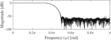
Figure 10: Example 2: Frequency responses $H_{n}(e^{j\omega})$, $n=0,1,\ldots,M-1$.

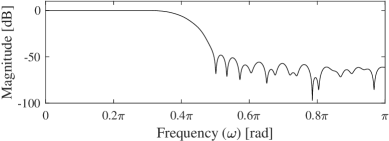
Figure 11: Example 2: Distortion frequency response $V_{0}(e^{j\omega})$ when using a reduced DFT length.

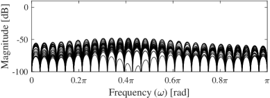
Figure 12: Example 2: Aliasing frequency responses $V_{p}(e^{j\omega})$, $p=1,2,\ldots,M-1$, when using a reduced DFT length.

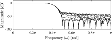
Figure 13: Example 2: Frequency responses $H_{n}(e^{j\omega})$, $n=0,1,\ldots,M-1$, when using a reduced DFT length.

Example 3: Periodic signals with frequencies matching the frequencies of a DFT of length $N/P$, can be efficiently time-domain interpolated through the use of a DFT and IDFT together with zero padding in the frequency domain. The basic principle is to, blockwise, compute a length-($N/P$) DFT of the input signal and then use the so obtained DFT coefficients as $N/P$ appropriately allocated nonzero-valued DFT coefficients, together with $N-N/P$ zero-valued DFT coefficients, in a length-$N$ DFT. Finally, a length-$N$ IDFT is computed, generating $N$ time-domain sample values, which corresponds to the original signal interpolated by $P$. Without quantized coefficients, the interpolation is error free for these periodic signals. However, when the signal is not periodic within a block of $N/P$ ($N$) samples before (after) the interpolation, large errors are introduced.

To illustrate the interpolation error for nonperiodic signals, it is first recognized that the scheme explained above is equivalent to first upsampling the signal by $P$, and then use the upsampled signal as the input to the overlap-add or overlap-save implementation with $N=L=M$ and with $H(k)=1$ ($H(k)=0$) for $k$-values corresponding to the nonzero-valued (zero-valued) DFT coefficients. For interpolated signals with frequencies between $2\pi k/N$, $k=0,1,\ldots,N-1$, large interpolation errors are introduced for two reasons. Firstly, the frequency response of the underlying filter, with the impulse response $h(n)$ obtained from the IDFT of $H(k)$, is poor between the frequencies $2\pi k/N$. This is illustrated in Fig. 14 for the case where $P=2$ and $N=32$. Secondly, since $N=L=M$, the length of the DFT, $N$, is shorter than required ($L+M-1$) for a proper implementation of linear convolution. This is seen in Figs. 15 and 16 which plot the distortion and aliasing functions, respectively. In a proper implementation ($N=L+M-1$) with unquantized coefficients, the aliasing functions are zero and the distortion function equals the frequency response of the underlying length-$L$ filter impulse response for all frequencies, not only for the frequencies $2\pi k/N$.

The two sources of errors for nonperiodic signals result in large interpolation errors. This is illustrated in Fig. 17 which plots the signal-to-noise-and distortion ratio (SNDR) as a function of frequency, when the input signal is a noisy sinusoid with a signal-to-noise ratio (SNR) of 80 dB. It is seen that for the frequencies $2\pi k/N$ (periodic signals), the SNDR is 80 dB as the interpolation is then error free and the SNDR determined by the SNR of the input signal. For frequencies between $2\pi k/N$ (nonperiodic signals), the SNDR is poor, especially around the mid-point between adjacent values of $2\pi k/N$ where it is only some $7$–$14$ dB. Figures 18 and 19 plot the spectrum for two of these signals, for the frequencies $2\pi\times 6/32$ and $2\pi\times 6.5/32$. As the plots show, the desired signal is obtained in the former of these two cases, whereas large aliasing terms are present in the latter, located at the signal frequency plus/minus multiples of $2\pi/N$. These errors match the large aliasing functions seen in Fig. 16. In order to use frequency-domain implementation of time-domain interpolation over the whole frequency range, it is thus necessary to properly design an interpolation filter and then implement the overlap-add or overlap-save method properly as in, e.g., [28].

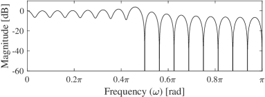
Figure 14: Example 3: Filter frequency response $H(e^{j\omega})$.

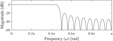
Figure 15: Example 3: Distortion frequency response $V_{0}(e^{j\omega})$.

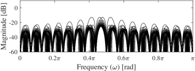
Figure 16: Example 3: Aliasing frequency responses $V_{p}(e^{j\omega})$, $p=1,2,\ldots,M-1$.

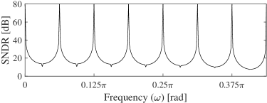
Figure 17: Example 3: SNDR as a function of the frequency of the interpolated signal.

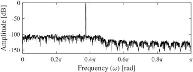
Figure 18: Example 3: Spectrum of the interpolated signal when its frequency is $2\pi\times 6/32$.

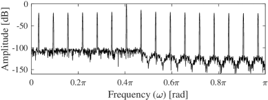
Figure 19: Example 3: Spectrum of the interpolated signal when its frequency is $2\pi\times 6.5/32$.

Table V: Multiplication Rates. Complex (Real) Means That Both the Signal and Impulse Response Are Complex-Valued (Real-Valued). Symmetric Means That the Impulse Response Is Symmetric (Not Conjugate Symmetric).

Case	Complex	Complex symmetric	Real	Real symmetric
Time-domain multiplication rate $R_{\textnormal{TD}}$	$3L$	$3\left\lceil L/2\right\rceil$	$L$	$\left\lceil L/2\right\rceil$
Frequency-domain multiplication rate $R_{\textnormal{FD}}$	$\frac{2(N\log_{2}(N)-3N/2+4)}{N-L+1}$	$\frac{2(N\log_{2}(N)-3N/2+4)}{N-L+1}$	$\frac{N\log_{2}(N)-3N/2+4}{N-L+1}$	$\frac{N\log_{2}(N)-3N/2+4}{N-L+1}$

VII Implementation Complexity

In this section, we will analyze and compare the computational complexities of the frequency-domain implementations and the corresponding time-domain implementations, assuming direct-form FIR filter structures [18, 19] for the latter. As a measure of computational complexity, we use the multiplication rate which is defined as the number of multiplications required to compute each output sample. The focus is here on multiplications as they are generally substantially more costly to implement than additions.

Earlier publications on the frequency-domain implementations indicate that they become more efficient than the corresponding time-domain implementations for filter lengths greater than $25$–$80$ for general FIR filters, and thus around $50$–$160$ for linear-phase FIR filters due to their impulse-response symmetries. However, as will be shown in this section, the frequency-domain implementations become more efficient for filter lengths far below those numbers. In part, this is because the use of more efficient FFT algorithms (in particular split-radix algorithms) can further reduce the complexity required to implement the DFT and IDFT. These further savings have been reported in other publications, e.g., in the context of chromatic-dispersion equalization [26] and sampling rate conversion [28]. However, here it will be shown that even further complexity savings are feasible using optimal DFT lengths which have not been used in earlier publications. A common selection has been a DFT length that is twice the filter length [26]. As will be seen later in this section, the optimal DFT length is around three times the filter length for short filters and it increases with the filter length. In particular, with optimal DFT lengths for general filters (without symmetries), we will show that the frequency-domain implementations are more efficient for all filter lengths. This was not seen in [28, 26] where short-length filters were reported to be more efficiently implemented in the time domain. It is noted though that [28] considers sampling rate conversions (by two in the examples), in which case the complexity expressions and analysis differ somewhat from the ones presented here.

VII-A Complexity Comparison

Table V gives the multiplication rate as a function of $N$ and $L$ for the frequency-domain and time-domain implementations, both for complex-valued and real-valued signals and impulse responses, and for general and symmetric impulse responses. For the complexity of the FFT and IFFT, we assume that each complex multiplication is implemented using three real multiplications. Assuming further that $N=2^{P}$, $P$ integer, and using split-radix algorithms, each of the FFT and IFFT can then be implemented with $N\log_{2}(N)-3N+4$ real multiplications for a complex-valued signal and impulse response [29, 30]. For a real-valued signal and impulse response, the number is halved [29, 30]. Further, the coefficients $H(k)$ require $3N$ multiplications in the complex case, but only $3N/2$ in the real case because the outputs of the FFT as well as $H(k)$ are then conjugate symmetric. Thus, for a real-valued signal and impulse response, the multiplication rate, say $R_{\textnormal{FD}}$, becomes

$$R_{\textnormal{FD}}=\frac{N\log_{2}(N)-3N/2+4}{N-L+1}.$$ (35)

For a complex-valued signal and impulse response, the multiplication rate is twice the right-hand side in (35).

Based on the expressions given in Table V, Fig. 20 plots the savings when using the frequency-domain implementations instead of the time-domain implementations for $L\in[2,256]$ (divided into two plots for visualization reasons). The saving in percent is given by $100\times(1-R_{\textnormal{FD}}/R_{\textnormal{TD}})$, where $R_{\textnormal{TD}}$ denotes the time-domain computational complexity. Further, for each value of $L$, the optimal saving has been obtained by minimizing $R_{\textnormal{FD}}$ over different $N=2^{P}\geq L$ and with $M=N-L+1$. Figure 20 shows that, for the general (unsymmetric) filters, the frequency-domain implementation is actually superior for all filter lengths. For symmetric filters, the frequency-domain implementations are computationally more efficient for filter lengths of $11$ and above in the real case, and more efficient for odd (even) filter lengths of $3$ ($6$) and above in the complex case.

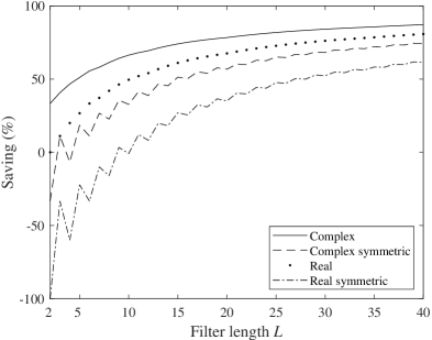
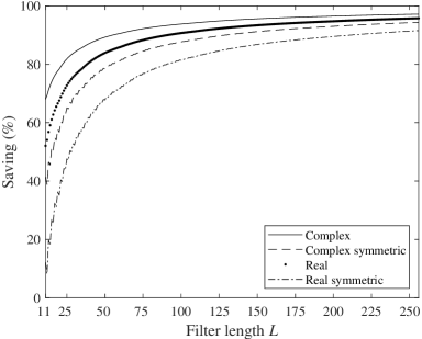
Figure 20: Example 4: Computational complexity savings using frequency-domain implementations instead of time-domain implementations. (It is divided into two plots for visualization reasons, and there is thus an overlap for $11\leq L\leq 40$).

VII-B Estimates of the Complexity

Figure 21 plots the complexities of the frequency-domain and time-domain implementations, corresponding to the upper plot in Fig. 20 (i.e., for $L\in[2,40]$). As can be seen, the computational complexities of the time-domain implementations grow linearly with $L$, in accordance with the expressions in Table V. For the frequency-domain implementation, the computational complexities are instead approximately proportional to $\log_{2}(L)$. A good estimation of the complexity for the real case is

$$\widehat{R}_{\textnormal{FD}}=\frac{\log_{2}(L)+\log_{2}(\log_{2}(L))-\frac{3}{2}+\frac{40}{9(L\times\log_{2}(L))}}{1-\frac{1}{\log_{2}(L)}+\frac{10}{9(L\times\log_{2}(L))}}.$$ (36)

This has been derived by inserting $N=0.9L\log_{2}(L)$ into (35) (see the motivation in the last paragraph of this section). Also recall that the computational complexity is twice as large in the complex case. Figure 22 plots the computational complexities of the frequency-domain implementations for $L\in[2,2^{12}]$ ($2^{12}=4096$) and the corresponding estimations based on (36). It is seen that the estimations are accurate for all values of $L$.

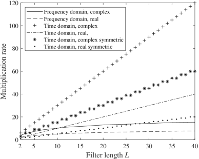
Figure 21: Example 4: Computational complexities using frequency-domain and time-domain implementations.

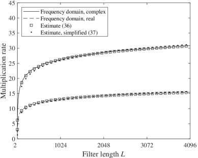
Figure 22: Example 4: Computational complexities using frequency-domain implementations.

From (36), one can deduce the simplified estimation

$$\widehat{R}_{\textnormal{FD}}=1.3\times\log_{2}(L),$$ (37)

which is also included in Fig. 22. It is seen that it is somewhat less accurate than the expression in (36), but it still gives a good approximation of the computational complexity and it shows that it is approximately proportional to $\log_{2}(L)$. This also explains the trend of the savings seen in Fig. 20 since the ratio $R_{\textnormal{FD}}/R_{\textnormal{TD}}$ is proportional to $\log_{2}(L)/L$ which approaches zero when $L$ increases. Thus, the savings approach one when $L$ increases.

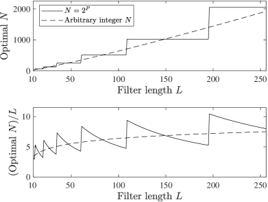
Figure 23: Example 4: DFT length $N$ versus filter length $L$.

Further, Fig. 23 plots the DFT length $N$ versus the filter length $L$, both for the case studied above with $N=2^{P}$ and when $N$ can take on all integers. Although the expression used for the multiplication rates, given by (35), holds only for $N=2^{P}$, the arbitrary-integer-$N$ case is also considered here for a comparison. As illustrated in Fig. 24, there is practically no difference between the two cases. In other words, the use of an arbitrary-integer-$N$ FFT algorithm, with a computational complexity as in (35), will not offer any further complexity reduction as the selection of the nearest $N$ satisfying $N=2^{P}$ results in practically the same computational complexity. The reason is that, for a given $L$, the function $R_{\textnormal{FD}}$ in (35) is flat over a large region around the optimal arbitrary-integer-$N$ case. This is exemplified in Fig. 25 for $L=128$.

Figure 24: Example 4: Computational complexity savings for $N=2^{P}$ and arbitrary integers $N$, and the difference between the savings.

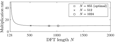
Figure 25: Example 4: Computational complexity versus DFT length $N$ with filter length $L=128$.

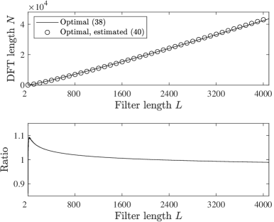
Figure 26: Example 4: Optimal DFT length $N$ and its estimate versus filter length $L$, and their ratio.

VII-C Estimate of the Optimal $N$

The optimal value of $N$, in the arbitrary-integer-$N$ case, can be obtained by setting the derivative of $R_{\textnormal{FD}}$ in (35) to zero and solve for $N$. This yields

$$N_{\textnormal{opt}} = (L-1)\ln(N_{\textnormal{opt}})+C$$ (38)

$$\approx (L-1)\ln(N_{\textnormal{opt}}),\quad L>L_{0},$$

where the constant $C$ is

$$C = (1-3\ln(2)/2)(L-1)+4\ln(2)$$ (39)

$$\approx -0.03972\times(L-1)+2.773,$$

which is much smaller than the term $(L-1)\ln(N_{\textnormal{opt}})$ in (38) for $L>L_{0}$. For example, with $L_{0}=8$ ($L_{0}=32$), the ratio between $C$ and $(L-1)\ln(N_{\textnormal{opt}})$ is less than $10$% ($1$%). We have solved equation (38) numerically using the Newton-Raphson method with the initial value $N_{\textnormal{opt}}^{(\textnormal{init})}=\hat{N}_{\textnormal{opt}}$, where the estimated optimal $N$ is

$$\widehat{N}_{\textnormal{opt}}=0.9L\log_{2}(L),$$ (40)

which is deduced from (38) and rather close to the optimum for practical values of $L$. This is illustrated in Fig. 26, where the optimal and estimated optimal values have been rounded to the nearest integers.

VIII Conclusion

This paper provided systematic derivations and analyses of MFB and PTVIR representations of frequency-domain implementations of FIR filters using the overlap-add and overlap-save techniques. As illustrated through design examples, including an interpolation example, these representations are useful when analyzing the effect of coefficient quantizations as well as the use of shorter DFT lengths than theoretically required. The examples also illustrated that the PTVIR representation is preferred when the worst-case time-domain error is more important than the average error which is captured by the MFB representation. The paper also provided detailed analysis of the lengths and and relations between the impulse responses in the PTVIR representation. It was shown that the overlap-add and overlap-save techniques have different properties when using quantized coefficients and shorter DFT lengths.

Finally, a computational-complexity analysis was provided, which showed that the frequency-domain implementations have lower computational complexities (multiplication rates) than the corresponding time-domain implementations for filter lengths that are shorter than reported earlier in the literature. In particular, for general (unsymmetric) filters, the frequency-domain implementations turn out to be more efficient for all filter lengths. For symmetric filters, the frequency-domain implementations are more efficient for filter lengths of $11$ and above in the real-signal-and-filter case, and more efficient for odd (even) filter lengths of $3$ ($6$) and above in the complex-signal-and-filter case. These results open up for new considerations when comparing complexities of different filter implementation alternatives.

References

- [1] A. V. Oppenheim and R. W. Schafer, Discrete-Time Signal Processing. Prentice Hall, 1989.
- [2] S. K. Mitra, Digital Signal Processing: A Computer-Based Approach. McGraw-Hill, 2006.
- [3] A. Eghbali, H. Johansson, O. Gustafsson, and S. J. Savory, “Optimal least-squares FIR digital filters for compensation of chromatic dispersion in digital coherent optical receivers,” IEEE/OSA J. Lightwave Technology, vol. 32, no. 8, pp. 1449–1456, Apr. 2014.
- [4] C. S. Martins, F. P. Guiomar, S. B. Amado, R. M. Ferreira, S. Ziaie, A. Shahpari, A. L. Teixeira, and A. N. Pinto, “Distributive FIR-based chromatic dispersion equalization for coherent receivers,” IEEE/OSA J. Lightwave Technology, vol. 34, no. 21, pp. 5023–5032, Nov. 2016.
- [5] A. Kovalev, O. Gustafsson, and M. Garrido, “Implementation approaches for 512-tap 60 GSa/s chromatic dispersion FIR filters,” in Proc. 51st Asilomar Conf. Signals, Syst., Computers, Pacific Grove, CA, USA, Oct. 29–Nov. 1, 2017, pp. 1779–1783.
- [6] C. Bae, M. Gokhale, O. Gustafsson, and M. Garrido, “Improved implementation approaches for 512-tap 60 GSa/s chromatic dispersion FIR filters,” in Proc. 52nd Asilomar Conf. Signals, Syst., Computers, Pacific Grove, Californa, USA, Oct. 28-31, 2018, pp. 213–217.
- [7] D. Wang, H. Jiang, G. Liang, Q. Zhan, Z. Su, and Z. Li, “Chromatic dispersion equalization FIR filter design based on discrete least-squares approximation,” Opt. Express, vol. 29, no. 13, pp. 20 387–20 394, June 2021.
- [8] C. Bae and O. Gustafsson, “Finite word length analysis for FFT-based chromatic dispersion compensation filters,” in Proc. OSA Advanced Photonics Congress, Washington DC, USA, July 26–29 2021.
- [9] C.-W. Liu, C.-K. Chan, P.-H. Cheng, and H.-Y. Lin, “FFT-based multirate signal processing for 18-band quasi-ansi s1.11 1/3-octave filter bank,” IEEE Trans. Circuits Syst. II: Express Briefs, vol. 66, no. 5, pp. 878–882, May 2019.
- [10] J. Nadal, F. Leduc-Primeau, C. A. Nour, and A. Baghdadi, “Overlap-save FBMC receivers,” IEEE Trans. Wireless Comm., vol. 19, no. 8, pp. 5307–5320, Aug. 2020.
- [11] R. De Gaudenzi, P. Angeletti, D. Petrolati, and E. Re, “Future technologies for very high throughput satellite systems,” Int. J. Satellite Comm. Networking, vol. 38, no. 2, pp. 141–161, Mar. 2020.
- [12] B. Kim, H. Yu, and S. Noh, “Cognitive interference cancellation with digital channelizer for satellite communication,” Sensors, vol. 20, no. 2, article 355, 2020.
- [13] S. Ruiz, T. Dietzen, T. Van Waterschoot, and M. Moonen, “A comparison between overlap-save and weighted overlap-add filter banks for multi-channel Wiener filter based noise reduction,” in Proc. 29th European Signal Processing Conference (EUSIPCO), Dublin, Ireland, Aug. 23-27, 2021, pp. 336–340.
- [14] X. X. Zheng, J. Yang, S. Y. Yang, W. Chen, L. Y. Huang, and X. Y. Zhang, “Synthesis of linear-phase FIR filters with a complex exponential impulse response,” IEEE Trans. Signal Processing, vol. 69, pp. 6101–6115, Sept. 2021.
- [15] A. K. M. Pillai and H. Johansson, “Efficient recovery of sub-Nyquist sampled sparse multi-band signals using reconfigurable multi-channel analysis and modulated synthesis filter banks,” IEEE Trans. Signal Processing, vol. 63, no. 19, pp. 5238–5249, Oct. 2015.
- [16] Y. Wang, H. Johansson, M. Deng, and Z. Li, “On the compensation of timing mismatch in two-channel time-interleaved ADCs: Strategies and a novel parallel compensation structure,” IEEE Trans. Signal Processing, vol. 70, pp. 2460–2475, May 2022.
- [17] A. Brihuega, L. Anttila, and M. Valkama, “Beam-level frequency-domain digital predistortion for OFDM massive MIMO transmitters,” IEEE Trans. Microwave Theory Techn., pp. 1–16, 2022 (early access).
- [18] L. B. Jackson, Digital Filters and Signal Processing (3rd Ed.). Kluwer Academic Publishers, 1996.
- [19] L. Wanhammar and H. Johansson, Digital Filters using Matlab. Linköping University, 2013.
- [20] P. P. Vaidyanathan, Multirate Systems and Filter Banks. Prentice Hall, 1993.
- [21] A. S. Mehr and T. Chen, “Representations of linear periodically time-varying and multirate systems,” IEEE Trans. Signal Processing, vol. 50, no. 9, pp. 2221–2229, Sept. 2002.
- [22] G. Burel, “Optimal design of transform-based block digital filters using a quadratic criterion,” IEEE Trans. Signal Processing, vol. 52, no. 7, pp. 1964–1974, July 2004.
- [23] A. Daher, E. H. Baghious, G. Burel, and E. Radoi, “Overlap-save and overlap-add filters: Optimal design and comparison,” IEEE Trans. Signal Processing, vol. 58, no. 6, pp. 3066–3075, June 2010.
- [24] H. Johansson and O. Gustafsson, “On frequency-domain implementation of digital FIR filters,” in Proc. IEEE Int. Conf. Digital Signal Processing., Singapore, July 21–24, 2015.
- [25] R. G. Lyons, Understanding Digital Signal Processing. Pearson, 1996.
- [26] K. Ishihara, R. Kudo, T. Kobayashi, A. Sano, Y. Takatori, T. Nakagawa, and Y. Miyamoto, “Frequency-domain equalization for coherent optical transmission systems,” in Optical Fiber Communication Conf. Exposition and National Fiber Optic Engineers Conf., Los Angeles, California, USA, Mar. 6–10 2011, pp. 1–3.
- [27] H. Johansson and P. Löwenborg, “Reconstruction of nonuniformly sampled bandlimited signals by means of time-varying discrete-time FIR filters,” J. Applied Signal Processing, Special Issue on Frames and Overcomplete Representations in Signal Processing, Communications, and Information Theory, vol. 2006, Article ID 64185, 2006.
- [28] S. Muramatsu and H. Kiya, “Extended overlap-add and -save methods for multirate signal processing,” IEEE Trans. Signal Processing, vol. 45, no. 9, pp. 2376–2380, Sept. 1997.
- [29] H. Sorensen, D. Jones, M. Heideman, and C. Burrus, “Real-valued fast Fourier transform algorithms,” IEEE Trans. Acoust., Speech, Signal Processing, vol. 35, no. 6, pp. 849–863, June 1987.
- [30] C. S. Burrus, M. Frigo, G. S. Johnson, M. Pueschel, and I. Selesnik, Fast Fourier Transforms. Samurai Media Limited, 2018.