An Optimal Projection Framework for Structure-Preserving Model Reduction of Linear Systems

Abstract

This paper presents a structure-preserving model reduction framework for linear systems, in which the $\mathcal{H}_{2}$ optimization is incorporated with the Petrov-Galerkin projection to preserve structural features of interest, including dissipativity, passivity, and bounded realness. The model reduction problem is formulated in a nonconvex optimization setting on a noncompact Stiefel manifold, aiming to minimize the $\mathcal{H}_{2}$ norm of the approximation error between the full-order and reduced-order models. The explicit expression for the gradient of the objective function is derived, and two gradient descent procedures are applied to seek for a (local) minimum, followed by a theoretical analysis on the convergence properties of the algorithms. Finally, the performance of the proposed method is demonstrated by two numerical examples which consider stability-preserving and passivity-preserving model reduction problems, respectively.

1 Introduction

Large-scale dynamical systems, including electric circuit design, structural mechanics, and microelectromechanical systems, are often described by considerably high-dimensional mathematical models and hence may require formidable computational demands for numerical simulations, control design, and optimization. This spurs the development of various model reduction techniques to generate lower-dimensional approximates, or reduced-order models, that allow us to capture the pertinent characteristics of large-scale systems in a computationally manageable fashion. These reduced-order models can further replace their complex counterparts in the control and optimization process, resulting in a shorter design cycle time, see [32, 4, 2, 17] for an overview.

Reduced-order models are often constructed to closely approximate the input-output mapping of original complex systems while preserving the essential structural features of large-scale systems presents a fundamental problem. Many physical systems possess certain properties or structural properties such as stability, passivity, or dissipativity, which are critical in determining the system behaviour and play a crucial role in the control and optimization of the systems. Hence, it is highly desirable that the reduced-order models also preserve the structural properties of the system and thereby provide an adequate and lean basis for control and optimization, retaining the physical characteristics, see e.g., [50, 56, 37, 12].

Structure-preserving model reduction has attracted extensive attention, and in the existing literature, different methods have been developed for reducing large-scale dynamical systems with specific structural properties. The balanced truncation approach [30] naturally retains system stability and minimality through a reduction process, which is extended to retain the positive real and bounded real properties of a linear system [17, 4, 36]. Further developments in e.g., [33, 20, 27, 50, 38, 9] extend the balanced truncation approach to preserve dissipativity or the port-Hamiltonian structure. The other model reduction methods, including moment matching or Krylov subspace approaches, generally do not guarantee to preserve stability, while the work in [16] shows that by combining the features of the singular value decomposition and Krylov-based approximation, the stability and moment matching can be achieved simultaneously. A generalization of this method is then presented in [43] by introducing the notions of contractivity and matrix measure. Furthermore, in e.g., [5, 44, 23, 19, 34, 49, 22, 21], the Krylov subspace approaches have been applied to the mode reduction of passive systems or port-Hamiltonian systems, where reduced-order models are produced with the preservation of the passivity and hence the stability. Besides, a reduction method for dissipative Hamiltonian systems is presented in [3], which adopts a symplectic time integrator to conserve the total energy of a Hamiltonian system. Although the aforementioned methods have demonstrated their effectiveness in structure-preserving model reduction, these methods barely guarantee any optimality with respect to a certain criterion. Furthermore, the methods based on the iterative rational Krylov algorithm (IRKA) do not guarantee convergence to local or global optima [14]. Recently, [42, 10] present new developments in passivity-preserving model reduction via techniques such as parameter optimization and spectral factorization.

In contrast to above methods, the works in e.g., [54, 46, 6, 7, 18, 41, 40, 39, 25, 31] formulate model reduction problem in the context of nonconvex $\mathcal{H}_{2}$ optimization, which aims to minimize the $\mathcal{H}_{2}$ error between original and reduced-order models. In [6, 7, 18], the first-order optimality conditions are evaluated on the basis of poles and residues of the transfer matrices of original and reduced-order models, and thereby the rational Krylov algorithm [6, 18] or the trust region method [7] can be applied to converge to a reduced-order model satisfying first-order optimality conditions with respect to the $\mathcal{H}_{2}$ error criteria. Nevertheless, structure preservation is not the primary concern of these methods. Within the pole-residue framework, [31] provides an optimal model reduction method that is capable to preserve the port-Hamiltonian structure, while this method is restricted to single-input and single-output systems.

The other nonconvex optimization framework for model reduction is formulated in e.g., [54, 41, 40, 39, 25] and the references therein. In this framework, the first-order conditions for (local) $\mathcal{H}_{2}$ optimality is established on coupled Lyapunov equations, and then gradient-based algorithms are devised to search for reduced-order models on the Stiefel manifold and Riemannian manifold, respectively, leading to structure-preserving reduced-order models. However, these methods in [54, 41, 40, 39] require the system state matrix or its symmetric part to be negative definite. The current paper follows this Lyapunov framework but requires only the stability of state matrices and hence can handle more general systems with different structural properties.

In this paper, we focus on the Petrov-Galerkin projection framework striving to find an optimal reduced-order model that not only admits the $\mathcal{H}_{2}$ optimality in reduction error but also preserves structural properties of interest. To this end, the $(Q,S,R)$-dissipativity of a linear state-space model is considered and characterized by a linear matrix inequality, whose solution is called a structure matrix and incorporated into constructing the project matrix. It can lead to certain degrees of freedom by altering the structure matrix to maintain desired structural properties including dissipativity, passivity, and bounded realness. Then, the model reduction problem is formulated as a nonconvex optimization on the basis of a noncompact Stiefel manifold. By using the controllability and observability Gramian matrices of the error system, we derive the explicit expression of the gradient of its objective function on the matrix manifold and provide two gradient descent algorithms to find a (local) optimal projection yielding the smallest reduction error. Unlike the previous works which only preserve one structural feature, this method allows retaining multiple structural properties in one unified framework by simply altering the structure matrix. Furthermore, compared to [54], we formulate the optimal projection problem on a noncompact Stiefel manifold that enables the algorithm to search the solutions in a larger topological space.

The paper is organized as follows. In Section 2 we recapitulate some preliminaries on the $\mathcal{H}_{2}$ norm and introduce the problem setting for the structure-preserving model reduction. The main results are presented in Section 3 and Section 4, where we formulate the model reduction problem in an optimization framework and solve it using gradient-based algorithms. The proposed methods are illustrated numerically in Section 5, and some concluding remarks are made in Section 6.

2 Preliminaries & Problem Setting

Some important notations and fundamental concepts are defined in this section, and the structure-preserving model reduction problem is then introduced.

2.1 Notations

The symbol $\mathbb{R}$ denotes the set of real numbers. For a matrix $A\in\mathbb{R}^{n\times m}$, the induced Frobenius norm of $A$ is denoted by $\|A\|^{2}_{F}=\langle A,A\rangle=\mathrm{Tr}(A^{\top}A)$. A symbol $\star$ in a square symmetric matrix stands for the symmetric counterpart, namely, we denote a symmetric matrix $\begin{bmatrix}A&B\\ B^{\top}&C\end{bmatrix}$ simply by $\begin{bmatrix}A&B\\ \star&C\end{bmatrix}$.

Let $\mathbb{S}^{n\times r}_{*}$ denote the set of all $n\times r$ matrices whose columns are linearly independent, i.e.

$$\mathbb{S}^{n\times r}_{*}=\{V\in\mathbb{R}^{n\times r}\mid\mathrm{Rank}(V)=r\}.$$ (1)

This is referred to as the manifold $\mathbb{S}^{n\times r}_{*}$, or the noncompact Stiefel manifold of full-rank $n\times r$ matrices. The set $\mathbb{S}^{n\times r}_{*}$ is an open subset of $\mathbb{R}^{n\times r}$ since its complement $\{X\in\mathbb{R}^{n\times r}:\det(X^{\top}X)=0\}$ is closed. Therefore, $\mathbb{S}^{n\times r}_{*}$ admits a structure of an open submanifold of $\mathbb{R}^{n\times r}$. We refer to [1] for more details.

2.2 Gramians and $\mathcal{H}_{2}$ Norm of Linear Stable Systems

We recapitulate the concept of the $\mathcal{H}_{2}$ norm of a stable linear time-invariant system with the following state-space representation.

$$\mathbf{\Sigma}:\ \begin{cases}\dot{x}(t)=Ax(t)+Bu(t),\\ y(t)=Cx(t)+Du(t),\end{cases}$$ (2)

where $x(t)\in\mathbb{R}^{n}$, $u(t)\in\mathbb{R}^{p}$, and $y(t)\in\mathbb{R}^{q}$ are the vectors of the states, inputs, and outputs of the system $\mathbf{\Sigma}$. $A\in\mathbb{R}^{n\times n}$, $B\in\mathbb{R}^{n\times p}$, $C\in\mathbb{R}^{q\times n}$, and $D\in\mathbb{R}^{q\times p}$ are constant matrices. If $A$ is Hurwitz, the system $\mathbf{\Sigma}$ is (asymptotically) stable. Then, the controllability and observability Gramians are properly defined as

$$\mathcal{P}=\int_{0}^{\infty}e^{At}BB^{\top}e^{A^{\top}t}\mathrm{d}{t},\quad\mathcal{Q}=\int_{0}^{\infty}e^{A^{\top}t}C^{\top}Ce^{At}\mathrm{d}{t},$$

respectively [4, 18]. Furthermore, the two positive semidefinite Gramian matrices are solved as unique solutions of the following Lyapunov equations:

$$A\mathcal{P}+\mathcal{P}A^{\top}+BB^{\top}=0,\quad A^{\top}\mathcal{Q}+\mathcal{Q}A+C^{\top}C=0.$$ (3)

Let the system $\mathbf{\Sigma}$ in (2) be strictly causal, i.e. $D=0$, and $G(s):=C(sI-A)^{-1}B$ be the transfer matrix of $\mathbf{\Sigma}$. Then, the $\mathcal{H}_{2}$ norm of $\mathbf{\Sigma}$ is defined and computed as

$$\|G(s)\|_{\mathcal{H}_{2}}^{2} =\int_{0}^{\infty}\mathrm{Tr}\left(Ce^{At}BB^{\top}e^{A^{\top}t}C^{\top}\right)\mathrm{d}{t}$$

$$=\mathrm{Tr}(C\mathcal{P}C^{\top})=\mathrm{Tr}(B^{\top}\mathcal{Q}B).$$

In this paper, the $\mathcal{H}_{2}$ norm is chosen to be a metric for evaluating the approximation accuracy of a reduced-order model such that an $\mathcal{H}_{2}$ optimal model reduction problem is formulated, where the objective function and its gradient can be formulated on the matrix manifold (1).

2.3 Structure-Preserving Model Reduction

The overall aim of this paper is to develop a general model reduction methodology that is applicable to a wide range of systems with specific structural properties, including passivity (or positive realness) and finite-gain $L_{2}$ stability (or bounded realness). To this end, we consider the concept of the $(Q,S,R)$-dissipativity, and the aforementioned structural properties can be considered as special cases of the $(Q,S,R)$-dissipativity.

Definition 1 ($(Q,S,R)$-Dissipativity).

[48, 11, 52, 51] For given matrices $Q=Q^{\top}$, $R=R^{\top}$ and $S$, a system $\mathbf{\Sigma}$ in (2) is called $(Q,S,R)$- dissipative if

$$\int_{0}^{\tau}y(t)^{\top}Qy(t)+u(t)^{\top}Ru(t)+2u(t)^{\top}Sy(t)\mathrm{d}{t}\geq 0$$ (4)

holds for all admissible $u(t)$ and all $\tau\geq 0$.

It is further shown in [48, 51, 28] that the $(Q,S,R)$-dissipativity of a linear state-space model (2) can be characterized by a linear matrix inequality.

Lemma 1.

A linear system (2) is $(Q,S,R)$-dissipative if and only if there exists a matrix $K>0$ such that

$$\Gamma=\begin{bmatrix}A^{\top}K+KA&KB-C^{\top}S&-C^{\top}Q^{\frac{1}{2}}\\ \star&-R-D^{\top}S-S^{\top}D&-D^{\top}Q^{\frac{1}{2}}\\ \star&\star&-I\end{bmatrix}\leq 0.$$ (5)

If $\Gamma$ is strictly negative definite, then the system (2) is asymptotically stable and $(Q,S,R)$-dissipative.

This work focuses on the notion of $(Q,S,R)$-dissipativity as it is a rather general property that can be reduced, with particular weighting matrices $Q$, $S$ and $R$, to passivity and finite-gain $L_{2}$ stability.

1. Let $Q=0$, $S=I$, $R=0$. Then, the $(Q,S,R)$-dissipativity reduces to the passivity (or positive realness) as $\int_{0}^{\tau}u(t)^{\top}y(t)\mathrm{d}{t}\geq 0$ for all admissible $u(t)$ and all $\tau\geq 0$. The inequality (5) is simplified as

   $$\begin{bmatrix}A^{\top}K+KA&KB-C^{\top}\\ \star&{-D^{\top}-D}\end{bmatrix}\leq 0,$$ (6)

2. Let $Q=-\gamma^{-1}I$, $S=0$, $R=\gamma I$, then the $(Q,S,R)$-dissipativity becomes the finite-gain $L_{2}$ stability (or bounded realness) as

   $$\int_{0}^{\tau}y(t)^{\top}y(t)\mathrm{d}{t}\leq\gamma^{2}\int_{0}^{\tau}u(t)^{\top}u(t)\mathrm{d}{t}$$

   for all admissible $u(t)$ and all $\tau\geq 0$, and meanwhile (5) is simplified by the Schur complement lemma as

   $$\begin{bmatrix}A^{\top}K+KA&KB\\ \star&-\gamma I\end{bmatrix}{+}\frac{1}{\gamma}\begin{bmatrix}C^{\top}\\ D^{\top}\end{bmatrix}\begin{bmatrix}C&D\end{bmatrix}\leq 0,$$ (7)

Remark 1.

We emphasize that the inequality in (5) only provides a characterization for the $(Q,S,R)$-dissipativity, which is a general concept including passivity and bounded realness. However, it is not necessary that the LMI in (5) has always to be solved numerically to obtain a solution of $K$. For instance, to reduce port-Hamiltonian systems as in e.g., [19, 34, 49, 22, 40, 25], we can simply use positive definite Hamiltonian matrices as $K$. To preserve the stability of an observable system, $K$ can be chosen as the observability Gramian of the system as in [16].

In this paper, we consider a full-order model $\mathbf{\Sigma}$ in (2), which is asymptotically stable and $(Q,S,R)$-dissipative, i.e. $A$, $B$, and $C$ satisfy the inequality (5). Then, the problem of structure-preserving model reduction in this paper is formulated as follows.

Problem 1.

Given a fixed positive integer $r$ ($<n$), we aim to construct a low-dimensional model

$$\mathbf{\hat{\Sigma}}:\ \begin{cases}\dot{\hat{x}}(t)=\hat{A}\hat{x}(t)+\hat{B}u(t),\\ \hat{y}(t)=\hat{C}\hat{x}(t)+\hat{D}u(t),\end{cases}$$ (8)

where $\hat{A}\in\mathbb{R}^{r\times r}$, $\hat{B}\in\mathbb{R}^{r\times p}$, $\hat{C}\in\mathbb{R}^{q\times r}$, and $\hat{D}\in\mathbb{R}^{q\times p}$ are reduced matrices such that

1. the reduction procedure guarantees the retention of the stability and the $(Q,S,R)$-dissipativity in the reduced-order model $\mathbf{\hat{\Sigma}}$, and

2. the reduced-order model $\mathbf{\hat{\Sigma}}$ best approximates the original model $\mathbf{\Sigma}$ in the sense that the $\mathcal{H}_{2}$ norm of the error between $\mathbf{\Sigma}$ and $\mathbf{\hat{\Sigma}}$ is minimized.

The objective (1) is to guarantee structural properties of interest retained in the reduced-order model. Under this constraint, the objective in (2) aims to minimize the approximation error in the $\mathcal{H}_{2}$ norm.

In this work, a unified framework will be presented to solve the structure-preserving model reduction problem, where the reduced-order model is built based on the Petrov-Galerkin projection. The model reduction problem thereby is reformulated as a nonconvex optimization problem, which is solved efficiently by a gradient descent method.

3 Projection-Based Model Reduction With Structure Preservation

Consider a full-order model in (2) with any structural property discussed in Section 2.3. To preserve the desired structure in the reduced-order model (8), a novel Petrov-Galerkin projection is adopted to generate a reduced-order model. Let $X=X^{\top}>0$, $V\in\mathbb{S}^{n\times r}_{*}$, and denote

$$V^{\dagger}:=(V^{\top}XV)^{-1}V^{\top}X,$$ (9)

in which $V^{\top}XV$ is invertible since $V$ has full column rank, and $X\in\mathbb{R}^{n\times n}$ is a positive definite matrix. $V^{\dagger}$ is called a reflexive generalized inverse of $V$. The projection matrix is thereby defined as $\Pi=VV^{\dagger}$, by which a reduced-order model is constructed as follows.

$$\mathbf{\hat{\Sigma}}:\ \begin{cases}\dot{\hat{x}}(t)=\underbrace{V^{\dagger}AV}_{\hat{A}}\hat{x}(t)+\underbrace{V^{\dagger}B}_{\hat{B}}u(t),\\ \hat{y}(t)=\underbrace{CV}_{\hat{C}}\hat{x}(t)+Du(t),\end{cases}$$ (10)

where $\hat{x}\in\mathbb{R}^{r}$ is the reduced state vector. The matrix $X$ is called a structure matrix, which allows us to preserve certain desired structural properties. The following result shows that this particular construction of a reduced-order model can lead to structure preservation.

Lemma 2 (Structure Preservation).

Consider the original system $\mathbf{\Sigma}$ (2) and its reduced-order model $\mathbf{\hat{\Sigma}}$ defined in (10). If $\mathbf{\Sigma}$ is $(Q,S,R)$-dissipative and $X=K>0$ in (10) is a solution of (5), then $\mathbf{\hat{\Sigma}}$ in (10) is also $(Q,S,R)$-dissipative.

Proof.

To verify the $(Q,S,R)$-dissipativity of the reduced-order model $\mathbf{\hat{\Sigma}}$ in (10), we let $\hat{K}=V^{\top}XV=V^{\top}KV$. Then, the following equations hold.

$$\hat{A}^{\top}\hat{K}+\hat{K}\hat{A}= V^{\top}A^{\top}XV+V^{\top}XAV$$

$$= V^{\top}(A^{\top}K+KA)V$$

$$\hat{K}\hat{B}-\hat{C}^{\top}S= V^{\top}(KB-C^{\top}S),$$

$$\hat{C}^{\top}Q^{\frac{1}{2}}= V^{\top}C^{\top}Q^{\frac{1}{2}}.$$

Based on that, we have

$$\begin{bmatrix}\hat{A}^{\top}\hat{K}+\hat{K}\hat{A}&\hat{K}\hat{B}-\hat{C}^{\top}S&-\hat{C}^{\top}Q^{\frac{1}{2}}\\ \star&-R-D^{\top}S-S^{\top}D&-D^{\top}Q^{\frac{1}{2}}\\ \star&\star&-I\end{bmatrix}$$

$$=\begin{bmatrix}V^{\top}&&\\ &I&\\ &&I\end{bmatrix}\Gamma\begin{bmatrix}V&&\\ &I&\\ &&I\end{bmatrix}\leq 0,$$

where $\Gamma$ defined in (5) is negative semidefinite due to the $(Q,S,R)$-dissipativity of the original model $\mathbf{\Sigma}$. Therefore, it follows from Lemma 1 that the reduced-order model $\mathbf{\hat{\Sigma}}$ remains $(Q,S,R)$-dissipative. ∎

Different structural properties can be preserved in the reduced-order model (10) by altering the structure matrix $X$. More preciously, let $X$ be the solution of (6), (7) or the inequality $AX+XA^{\top}<0$, we can retain passivity, finite-gain $L_{2}$ stability, or stability, respectively. Therefore, a unified framework is presented here to address the model reduction problems with different structural constraints. Particularly, this work provides a novel method for the passivity-preserving model reduction problems for port-Hamiltonian systems, which have been extensively studied in the literature, see e.g., [5, 23, 19, 34, 49, 22, 21, 33, 38, 40, 31]. In our approach, the structure matrix $X$ in (9) can be chosen as the energy matrix $K$ of the system i.e. $\frac{1}{2}x(t)^{\top}Kx(t)$ represents the total energy (Hamiltonian) of the system. Consequently, the reduced-order model has the reduced energy matrix as $V^{\top}KV$.

Remark 2 (Multiple Structural Properties).

The proposed model reduction framework can also be applied to preserve multiple structural properties, while $X$ in (9) is required to be a common solution of the corresponding matrix inequalities or equations. For instance, if there exists $K$ satisfying (6) and (7) simultaneously, then we let $X=K$ in (9) that preserves the passivity and finite-gain $L_{2}$ stability in the reduced-order model (10).

Remark 3.

Instead of the $(Q,S,R)$-dissipativity, we may consider retaining controllability or observability of a given system $\mathbf{\Sigma}$. In this regard, we let the structure matrix $X$ be the solution of

$$A^{\top}X+XA+XBB^{\top}X=0,$$

or

$$A^{\top}X+XA+C^{\top}C=0,$$

using which to construct a reduced-order model (10) will allow the preservation of controllability or observability. Furthermore, if $X$ is chosen as the observability Gramian of the system $\mathbf{\Sigma}$, then the stability is simultaneously preserved in the reduced-order model (10) [16].

The reduced-order model in (10) guarantees the preservation of a desirable structural property by selecting a specific matrix $X$. Next, we aim to minimize the approximation error between the original and reduced models by tuning $V$. To this end, we define the error system as

$$G_{e}(s)=C(sI_{n}-A)^{-1}B-CV(sI_{r}-V^{\dagger}AV)^{-1}V^{\dagger}B,$$

where the feedthrough gain $D$ in the two systems has been canceled out. The system $G_{e}(s)$ has the following state-space representation

$$\begin{cases}\dot{z}(t)={A}_{e}z(t)+{B}_{e}u(t)\\ y_{e}(t)={C}_{e}z(t)\end{cases}$$ (11)

where $z(t)=[x(t)^{\top}\ \hat{x}(t)^{\top}]^{\top}\in\mathbb{R}^{n+r}$, and

$${A}_{e}=\begin{bmatrix}A&0\\ 0&V^{\dagger}AV\end{bmatrix},\ {B}_{e}=\begin{bmatrix}B\\ V^{\dagger}B\end{bmatrix},\ {C}_{e}=\begin{bmatrix}C&-CV\end{bmatrix}.$$

To guarantee the stability of the error system, we consider the original system $\mathbf{\Sigma}$ asymptotically stable, i.e. $A$ in (2) is Hurwitz. Thereby, let the structure matrix $X$ additionally be a solution of $\Gamma<0$, instead of $\Gamma\leq 0$ in (5). Note that $\Gamma<0$ implies

$$A^{\top}X+XA<0,$$

which will impose the asymptotic stability of the reduced-order model $\mathbf{\hat{\Sigma}}$. Then, the square $\mathcal{H}_{2}$-norm of the approximation error is computed as

$$\|G_{e}(s)\|_{\mathcal{H}_{2}}^{2}=\mathrm{Tr}(C_{e}\mathcal{P}C_{e}^{\top})=\mathrm{Tr}(B_{e}^{\top}\mathcal{Q}B_{e}),$$ (12)

where $\mathcal{P}$ and $\mathcal{Q}$ are the controllability and observability Gramians of the error system (11). Algebraically, $\mathcal{P}$ and $\mathcal{Q}$ are solved as the unique solutions of the following Lyapunov equations:

$$A_{e}\mathcal{P}+\mathcal{P}A_{e}^{\top}+B_{e}B_{e}^{\top} =0,$$ (13a)

$$A_{e}^{\top}\mathcal{Q}+\mathcal{Q}A_{e}+C_{e}^{\top}C_{e} =0.$$ (13b)

Observe that given a structure matrix $X$, the reduced-order model (10) is parameterized in the matrix $V$. We formulate an optimization problem in terms of minimizing the $\mathcal{H}_{2}$ norm of the error system $G_{e}(s)$:

$$\min_{V,\mathcal{Q}}\;\mathrm{Tr}(B_{e}^{\top}\mathcal{Q}B_{e})$$ (14)

$$\;\;\text{s.t.:}\;\;V^{\top}V>0,\quad V\in\mathbb{R}^{n\times r},$$

$$\;\;\quad\quad A_{e}^{\top}\mathcal{Q}+\mathcal{Q}A_{e}+C_{e}^{\top}C_{e}=0.$$

This optimization problem is highly nonconvex and has a continuous variable $\mathcal{Q}\in{\mathbb{R}}^{(n+r)\times(n+r)}$ and a full column rank matrix $V\in\mathbb{R}_{*}^{n\times r}$, where $\mathcal{Q}=\mathcal{Q}(V)$ is an implicit function of $V$ due to the unique solution of the Lyapunov equation (13b). Hence, for any $V\in\mathbb{R}_{*}^{n\times r}$, the partial minimization in $\mathcal{Q}$ leads to the optimization problem

$$\min_{V\in\mathbb{S}^{n\times r}_{*}}\;J(V)\;: =\mathrm{Tr}\left(B_{e}(V)^{\top}\mathcal{Q}(V)B_{e}(V)\right)$$ (15)

$$=\mathrm{Tr}\left(\mathcal{Q}(V)B_{e}(V)B_{e}(V)^{\top}\right),$$

where the set $\mathbb{S}^{n\times r}_{*}$ is defined in (1).

4 Gradient-Based Methods for Optimal Projection

This section presents gradient-based methods for solving the model reduction problem as a nonconvex optimization problem. The explicit expression for the gradient of the objective function $J(V)$ is derived, and furthermore, gradient descent algorithms are proposed to minimize $J(V)$ over both noncompact and compact Stiefel manifolds.

4.1 Gradient Analysis

To solve the optimization problem (15), we analyze the key properties of the objective function $J(V)$ such as smoothness and differentiability, based on which we can apply gradient-based methods for solving (15) over the manifold $\mathbb{S}^{n\times r}_{*}$. In particular, we show in the next theorem that $J$ is a differentiable function and derive an explicit expression for its gradient. Before proceeding, we partition the controllability and observability Gramians $\mathcal{P}$ and $\mathcal{Q}$ according to the block structure of the error system as:

$$\mathcal{P}=\begin{bmatrix}\mathcal{P}_{11}&\mathcal{P}_{12}\\ \mathcal{P}_{12}^{\top}&\mathcal{P}_{22}\end{bmatrix},\quad\mathcal{Q}=\begin{bmatrix}\mathcal{Q}_{11}&\mathcal{Q}_{12}\\ \mathcal{Q}_{12}^{\top}&\mathcal{Q}_{22}\end{bmatrix},$$ (16)

where $P_{11}$ and $Q_{11}$ are Gramians of the high-order system (2), and $P_{22}$ and $Q_{22}$ are the Gramians of the reduced-order model (10). Here, the submatrices $\mathcal{P}_{22}$, $\mathcal{Q}_{22}$, $\mathcal{P}_{12}$, and $\mathcal{Q}_{12}$ are characterized by the following Sylvester equations:

$$\hat{A}\mathcal{P}_{22}+\mathcal{P}_{22}\hat{A}^{\top}+\hat{B}\hat{B}^{\top}=0,$$ (17a)

$$\hat{A}^{\top}\mathcal{Q}_{22}+\mathcal{Q}_{22}\hat{A}+\hat{C}^{\top}\hat{C}=0,$$ (17b)

$${A}\mathcal{P}_{12}+\mathcal{P}_{12}\hat{A}^{\top}+{B}\hat{B}^{\top}=0,$$ (17c)

$${A}^{\top}\mathcal{Q}_{12}+\mathcal{Q}_{12}\hat{A}-{C}^{\top}\hat{C}=0,$$ (17d)

where $\hat{A}$, $\hat{B}$, and $\hat{C}$ are computed as in (10). Then, the following theorem holds.

Theorem 1 (Gradient on Matrix Manifold).

The objective function $J(V)$ in (15) is differentiable, and the gradient has the following expression:

$$\nabla J(V)= 2X(I-VV^{\dagger})\left[\mathcal{F}_{A}(V)+\mathcal{F}_{B}(V)^{\top}\right](V^{\top}XV)^{-1}$$

$$-2(V^{\dagger})^{\top}\left[\mathcal{F}_{A}(V)^{\top}+\mathcal{F}_{B}(V)\right](V^{\dagger})^{\top}$$

$$+2A^{\top}(V^{\dagger})^{\top}\Sigma_{22}^{\top}+2\mathcal{F}_{C}(V),$$ (18)

where $\Sigma_{22}:=\mathcal{P}_{12}^{\top}\mathcal{Q}_{12}+\mathcal{P}_{22}\mathcal{Q}_{22}$, and

$$\mathcal{F}_{A}(V): =AV\Sigma_{22},$$ (19a)

$$\mathcal{F}_{B}(V): =\mathcal{Q}_{12}^{\top}BB^{\top}+\mathcal{Q}_{22}V^{\dagger}BB^{\top},$$ (19b)

$$\mathcal{F}_{C}(V): =C^{\top}CV\mathcal{P}_{22}-C^{\top}C\mathcal{P}_{12}.$$ (19c)

Proof.

Observe that $V^{\top}X=(V^{\top}XV)V^{\dagger}.$ We take the differential on both sides, leading to

$$\mathrm{d}V^{\top}X= \mathrm{d}((V^{\top}XV)V^{\dagger})$$

$$= \mathrm{d}(V^{\top}XV)V^{\dagger}+(V^{\top}XV)\mathrm{d}V^{\dagger}$$

$$= (\mathrm{d}V^{\top}XV+V^{\top}X\mathrm{d}V)V^{\dagger}+(V^{\top}XV)\mathrm{d}(V^{\dagger}),$$

from which, the differential $\mathrm{d}(V^{\dagger})$ is solved as

$$\mathrm{d}(V^{\dagger})=(V^{\top}XV)^{-1}\mathrm{d}V^{\top}X(I-VV^{\dagger})-V^{\dagger}\mathrm{d}VV^{\dagger}.$$ (20)

To compute the gradient $\nabla J(V)$, we write the derivative $J^{\prime}(V)\mathrm{d}{V}$ for some $\mathrm{d}{V}\in\mathbb{R}^{n\times r}$ in a gradient form in terms of trace as follows.

$$J^{\prime}(V)\mathrm{d}{V}=\mathrm{Tr}\left(\nabla J(V)^{\top}\mathrm{d}{V}\right).$$

Considering (15), $J^{\prime}(V)\mathrm{d}{V}$ can be specified as

$$J^{\prime}(V)\mathrm{d}{V} =\mathrm{Tr}\left(\mathcal{Q}(V)\mathrm{d}{\mathcal{B}}(V)+\mathrm{d}\mathcal{Q}(V){\mathcal{B}}(V)\right)$$

$$=\mathrm{Tr}\left(\mathcal{Q}(V)\mathrm{d}{\mathcal{B}}(V)\right)+\mathrm{Tr}\left(\mathrm{d}\mathcal{Q}(V){\mathcal{B}}(V)\right),$$ (21)

where ${\mathcal{B}}(V)$ is denoted for notational simplicity as

$$\mathcal{B}(V)=B_{e}B_{e}^{\top}=\begin{bmatrix}BB^{\top}&BB^{\top}(V^{\dagger})^{\top}\\ V^{\dagger}BB^{\top}&V^{\dagger}BB^{\top}(V^{\dagger})^{\top}\end{bmatrix}.$$ (22)

In the following, the two terms in (4.1) are computed separately.

First, we analyze the first term in (4.1). From (22), it follows that

$$\mathrm{d}\mathcal{B}(V)=\begin{bmatrix}0&BB^{\top}\mathrm{d}(V^{\dagger})^{\top}\\ \mathrm{d}(V^{\dagger})BB^{\top}&\mathrm{d}(\hat{B}\hat{B}^{\dagger})\end{bmatrix},$$

where $\mathrm{d}(\hat{B}\hat{B}^{\dagger})=\mathrm{d}(V^{\dagger})BB^{\top}(V^{\dagger})^{\top}+V^{\dagger}BB^{\top}\mathrm{d}(V^{\dagger})^{\top}$. Thus, the first term in (4.1) can be specified as

$$\mathrm{Tr}\left(\mathcal{Q}(V)\mathrm{d}\mathcal{B}(V)\right)$$ (23)

$$= \mathrm{Tr}\left(\mathcal{Q}_{12}\mathrm{d}(V^{\dagger})BB^{\top}+\mathcal{Q}_{12}^{\top}BB^{\top}\mathrm{d}(V^{\dagger})^{\top}\right.$$

$$\left.\quad+\mathcal{Q}_{22}\mathrm{d}(V^{\dagger})BB^{\top}(V^{\dagger})^{\top}+\mathcal{Q}_{22}V^{\dagger}BB^{\top}\mathrm{d}(V^{\dagger})^{\top}\right).$$

Using the standard properties of trace, we have

$$\mathrm{Tr}\left(\mathcal{Q}_{12}\mathrm{d}(V^{\dagger})BB^{\top}\right) =\mathrm{Tr}\left(BB^{\top}\mathrm{d}(V^{\dagger})^{\top}\mathcal{Q}_{12}^{\top}\right)$$

$$=\mathrm{Tr}\left(\mathcal{Q}_{12}^{\top}BB^{\top}\mathrm{d}(V^{\dagger})^{\top}\right),$$

and

$$\mathrm{Tr}\left(\mathcal{Q}_{22}\mathrm{d}(V^{\dagger})BB^{\top}(V^{\dagger})^{\top}\right) =\mathrm{Tr}\left(V^{\dagger}BB^{\top}\mathrm{d}(V^{\dagger})^{\top}\mathcal{Q}_{22}\right)$$

$$=\mathrm{Tr}\left(\mathcal{Q}_{22}V^{\dagger}BB^{\top}\mathrm{d}(V^{\dagger})^{\top}\right).$$

Consequently, (23) is simplified as

$$\mathrm{Tr}\left(\mathcal{Q}(V)\mathrm{d}\mathcal{B}(V)\right)=2\mathrm{Tr}\left(\mathcal{F}_{B}(V)\mathrm{d}(V^{\dagger})^{\top}\right).$$

with $\mathcal{F}_{B}(V)$ defined in (19b). Substituting the differential of $\mathrm{d}(V^{\dagger})$ in (20) into the above equation then yields

$$\mathrm{Tr}\left(\mathcal{Q}(V)\mathrm{d}\mathcal{B}(V)\right)$$ (24)

$$= 2\mathrm{Tr}\left[\mathcal{F}_{B}(V)(I-(VV^{\dagger})^{\top})X\mathrm{d}V(V^{\top}XV)^{-1}\right.$$

$$\left.\quad-\mathcal{F}_{B}(V)(V^{\dagger})^{\top}\mathrm{d}(V)^{\top}(V^{\dagger})^{\top}\right]$$

$$= 2\mathrm{Tr}\left[(V^{\top}XV)^{-1}\mathcal{F}_{B}(V)(I-(VV^{\dagger})^{\top})X\mathrm{d}V\right.$$

$$\left.\quad-V^{\dagger}\mathcal{F}_{B}(V)^{\top}V^{\dagger}\mathrm{d}V\right].$$

Next, we derive an explicit expression for the second term in (4.1), i.e. $\mathrm{Tr}\left(\mathrm{d}\mathcal{Q}(V){\mathcal{B}}(V)\right)$. To this end, we define the function:

$$\Phi(V,\mathcal{Q})=A_{e}^{\top}\mathcal{Q}+\mathcal{Q}A_{e}+\mathcal{C}(V)=0,$$ (25)

whose partial derivatives with respect to $V$ and $\mathcal{Q}$ are given as

$$\Phi_{V}^{\prime}(V,\mathcal{Q})\mathrm{d}{V}=(\mathrm{d}A_{e}(V))^{\top}{\mathcal{Q}}+{\mathcal{Q}}\mathrm{d}A_{e}(V)+\mathrm{d}\mathcal{C}(V),$$

and

$$\Phi_{\mathcal{Q}}^{\prime}(V,\mathcal{Q})\mathrm{d}{\mathcal{Q}}=(A_{e}(V))^{\top}\mathrm{d}{\mathcal{Q}}+\mathrm{d}{\mathcal{Q}}A_{e}(V),$$

where

$$\mathcal{C}(V)=C_{e}^{\top}C_{e}=\begin{bmatrix}C^{\top}C&-C^{\top}CV\\ -V^{\top}C^{\top}C&V^{\top}C^{\top}CV\end{bmatrix}.$$ (26)

Since $\Phi(V,\mathcal{Q})$ a multivariable function of both $V$ and $\mathcal{Q}$ and $\Phi(V,\mathcal{Q})=0$, applying the Implicit Function Theorem yields $\Phi_{V}^{\prime}(V,\mathcal{Q})\mathrm{d}{V}+\Phi_{\mathcal{Q}}^{\prime}(V,\mathcal{Q})\mathrm{d}{\mathcal{Q}}=0$, i.e.

$$(\mathrm{d}A_{e})^{\top}\mathcal{Q}(V)+\mathcal{Q}(V)\mathrm{d}A_{e}(V)+\mathrm{d}\mathcal{C}(V)\\ +(A_{e}(V))^{\top}\mathrm{d}{\mathcal{Q}}(V)+\mathrm{d}{\mathcal{Q}}(V)A_{e}(V)=0.$$

Multiplying $\mathcal{P}(V)$ from the left then gives

$$\mathcal{P}(\mathrm{d}A_{e})^{\top}\mathcal{Q}+\mathcal{P}\mathcal{Q}\mathrm{d}A_{e}+\mathcal{P}\mathrm{d}\mathcal{C}\\ +\mathcal{P}A_{e}^{\top}\mathrm{d}{\mathcal{Q}}+\mathcal{P}\mathrm{d}{\mathcal{Q}}A_{e}=0,$$ (27)

where we suppress the dependence on $V$ for ease of notation. Furthermore, notice that the controllability Gramian $\mathcal{P}(V)$ is the unique solution of the Lyapunov equation (13a), from which we obtain

$$A_{e}\mathcal{P}\mathrm{d}{\mathcal{Q}}+\mathcal{P}A_{e}^{\top}\mathrm{d}{\mathcal{Q}}=-\mathcal{B}\mathrm{d}{\mathcal{Q}}.$$ (28)

Subtracting (28) from (27) leads to

$$\mathcal{P}A_{e}^{\top}\mathrm{d}{\mathcal{Q}}+\mathcal{P}\mathrm{d}{\mathcal{Q}}A_{e}-A_{e}\mathcal{P}\mathrm{d}{\mathcal{Q}}-\mathcal{P}A_{e}^{\top}\mathrm{d}{\mathcal{Q}}\\ +\mathcal{P}(\mathrm{d}A_{e})^{\top}\mathcal{Q}+\mathcal{P}\mathcal{Q}\mathrm{d}A_{e}-\mathcal{B}\mathrm{d}{\mathcal{Q}}+\mathcal{P}\mathrm{d}\mathcal{C}=0.$$

Then, we take the trace in the above equation that cancels the first four terms and yields an expression for the first term in (4.1) as

$$\mathrm{Tr}\left(\mathrm{d}\mathcal{Q}\mathcal{B}\right)=2\mathrm{Tr}\left(\mathcal{P}\mathcal{Q}\mathrm{d}A_{e}\right)+\mathrm{Tr}\left(\mathcal{P}\mathrm{d}\mathcal{C}\right),$$ (29)

where

$$\mathrm{d}A_{e}(V)=\begin{bmatrix}0&0\\ 0&\mathrm{d}\hat{A}(V)\end{bmatrix},$$

with $\mathrm{d}\hat{A}(V)=\mathrm{d}(V^{\dagger}AV)=\mathrm{d}(V^{\dagger})AV+V^{\dagger}A\mathrm{d}V$. Applying (20), we therefore obtain

$$\mathrm{Tr}\left(\mathcal{P}\mathcal{Q}\mathrm{d}A_{e}\right)$$ (30)

$$= \mathrm{Tr}\left[\Sigma_{22}\mathrm{d}(V^{\dagger})AV+\Sigma_{22}V^{\dagger}A\mathrm{d}V\right]$$

$$= \mathrm{Tr}\left[\Sigma_{22}(V^{\top}XV)^{-1}\mathrm{d}V^{\top}X(I-VV^{\dagger})AV\right.$$

$$\quad\left.-\Sigma_{22}V^{\dagger}\mathrm{d}VV^{\dagger}AV+\Sigma_{22}V^{\dagger}A\mathrm{d}V\right]$$

$$= \mathrm{Tr}\left[(V^{\top}XV)^{-1}\mathcal{F}_{A}(V)^{\top}(I-(VV^{\dagger})^{\top})X\mathrm{d}V\right.$$

$$\quad\left.-V^{\dagger}\mathcal{F}_{A}(V)V^{\dagger}\mathrm{d}V+\Sigma_{22}V^{\dagger}A\mathrm{d}V\right],$$

with $\mathcal{F}_{A}(V)$ defined in (19a). Moreover, taking into account the structure of $\mathcal{C}(V)$ in (26), we expand the second term in (29) as

$$\mathrm{Tr}(\mathcal{P}\mathrm{d}\mathcal{C})$$ (31)

$$= -\mathrm{Tr}(\mathcal{P}_{12}\mathrm{d}{V}^{\top}C^{\top}C)-\mathrm{Tr}(\mathcal{P}_{12}^{\top}C^{\top}C\mathrm{d}{V})$$

$$+\mathrm{Tr}\left[\mathcal{P}_{22}(\mathrm{d}{V}^{\top}C^{\top}CV+{V}^{\top}C^{\top}C\mathrm{d}V)\right]$$

$$= 2\mathrm{Tr}(-\mathcal{P}_{12}^{\top}C^{\top}C\mathrm{d}{V}+\mathcal{P}_{22}{V}^{\top}C^{\top}C\mathrm{d}V)$$

$$= 2\mathrm{Tr}(\mathcal{F}_{C}(V)^{\top}\mathrm{d}{V}).$$

Finally, we combine the three equations in (24), (30), and (31) to obtain the gradient in (1) ∎

Remark 4.

Different from methods in from e.g., [46, 40], which provide three gradient expressions over the variables $\hat{A}$, $\hat{B}$, and $\hat{C}$, respectively, this paper aims to find the optimal reduced basis matrix $V$ for projection, which is the only optimization variable in the optimization problem (15). Theorem 1 thereby provides the expression of the gradient over $V$, which is clearly different from the aforementioned methods.

Remark 5.

Note that the computation of the gradient $\nabla J$ does not need the Gramian matrices $\mathcal{P}_{11}\in\mathbb{R}^{n\times n}$ and $\mathcal{Q}_{11}\in\mathbb{R}^{n\times n}$ of the original system. It only requires to compute the Gramians for the reduced-order model $\mathcal{P}_{22}\in\mathbb{R}^{r\times r}$, $\mathcal{Q}_{22}\in\mathbb{R}^{r\times r}$ and the cross terms $\mathcal{P}_{12}\in\mathbb{R}^{n\times r}$, $\mathcal{Q}_{12}\in\mathbb{R}^{n\times r}$. The computation of $\mathcal{P}_{22}$ and $\mathcal{Q}_{22}$ can be efficient as the reduced order $r$ is typically small in model reduction problems. Nevertheless, solving the Sylvester equations in (17) can still be computationally demanding due to (17c) and (17d) that contain the matrices from the original system. To make the computation of $\mathcal{P}_{12}$ and $\mathcal{Q}_{12}$ more tractable, we follow [45] and derive explicit expressions for $\mathcal{P}_{12}$ and $\mathcal{Q}_{12}$ as the sums of rank-one matrices:

$$\mathcal{P}_{12} =\sum_{j=1}^{r}(\mu_{j}I_{r}+{A})^{-1}B\hat{B}^{\top}w_{j}\hat{w}_{j}^{*},$$ (32a)

$$\mathcal{Q}_{12} =\sum_{j=1}^{r}(\mu_{j}I_{r}+{A}^{\top})^{-1}{C}\hat{C}^{\top}\hat{w}_{j}w_{j}^{*},$$ (32b)

where the vectors $w_{j}$ and $\hat{w}_{j}$ are the right and left eigenvectors corresponding to the eigenvalue $\mu_{j}$ of $\hat{A}$, respectively. Computing (32) now requires the eigendecomposition of the reduced matrix $\hat{A}$ followed by $r$ inversions of $n\times n$ matrices $\mu_{j}I+A$, which may be less expensive than directly applying standard Sylvester equation solvers, particularly when $A$ is sparse, and $r$ is small. To further accelerate the method, it is advisable to adopt a low-rank method, see e.g., [24, 8], to achieve approximate solutions with cheap computations for extremely large-scale systems.

Having the formula for the gradient $\nabla J$ in (1), we further define a gradient flow of $J(V)$ as

$$\frac{\mathrm{d}}{\mathrm{d}t}{V}(t)= -2X(I-VV^{\dagger})\left[\mathcal{F}_{A}(V)+\mathcal{F}_{B}(V)^{\top}\right](V^{\top}XV)^{-1}$$

$$+2(V^{\dagger})^{\top}\left[\mathcal{F}_{A}(V)^{\top}+\mathcal{F}_{B}(V)\right](V^{\dagger})^{\top}$$

$$-2A^{\top}(V^{\dagger})^{\top}\Sigma_{22}^{\top}-2\mathcal{F}_{C}(V),$$ (33)

with $\mathcal{F}_{A}(V)$, $\mathcal{F}_{B}(V)$, and $\mathcal{F}_{C}(V)$ defined in (19), and then we analyze the key properties of the gradient flow.

Theorem 2.

Let the initial condition of (4.1) be given by $V(0)=V_{0}\in\mathbb{S}^{n\times r}_{*}$. Then, the following statements hold.

1. $V(t)^{\top}\frac{\mathrm{d}}{\mathrm{d}t}{V(t)}=0$, and $V(t)^{\top}V(t)$ is invariant in the gradient flow (4.1).

2. $V(t)\in\mathbb{S}^{n\times r}_{*}$ for all $t\geq 0$.

3. The objective function is nonincreasing along $V(t)$ with

   $$J(V(t_{1}))\geq J(V(t_{2})),$$ (34)

   for all $0\leq t_{1}\leq t_{2}$.

4. Let $V$ be any local minimizer of problem (15), the following implication holds

   $$\nabla J(V)=0\ \Leftrightarrow\ \nabla J(V)V^{\top}-V\nabla J(V)^{\top}=0.$$ (35)

Proof.

We first prove $V^{\top}\frac{\mathrm{d}}{\mathrm{d}t}{V}=0$ for any $V\in\mathbb{S}^{n\times r}_{*}$. We rewrite (4.1) as $\frac{\mathrm{d}}{\mathrm{d}t}{V}=2(\mathcal{J}_{1}+\mathcal{J}_{2})$, where

$$\mathcal{J}_{1}= -X(I-VV^{\dagger})\left[\mathcal{F}_{A}(V)+\mathcal{F}_{B}(V)^{\top}\right](V^{\top}XV)^{-1},$$

$$\mathcal{J}_{2}= (V^{\dagger})^{\top}\left[\mathcal{F}_{A}(V)^{\top}+\mathcal{F}_{B}(V)\right](V^{\dagger})^{\top}$$

$$-A^{\top}(V^{\dagger})^{\top}\Sigma_{22}^{\top}-\mathcal{F}_{C}(V),$$

Note that $V^{\top}X(I-VV^{\dagger})=V^{\top}X-V^{\top}XVV^{\dagger}=0,$ which leads to

$$V^{\top}\mathcal{J}_{1}=0.$$ (36)

Furthermore, we have

$$V^{\top}\mathcal{J}_{2}= \Sigma_{22}^{\top}\hat{A}+\mathcal{Q}_{12}^{\top}B\hat{B}^{\top}+\mathcal{Q}_{22}\hat{B}\hat{B}^{\top}$$

$$-\hat{A}^{\top}\Sigma_{22}-\hat{C}^{\top}\hat{C}\mathcal{P}_{22}+\hat{C}^{\top}C\mathcal{P}_{12}$$ (37)

and it is obtained from the Sylvester equations in (17) that

$$-\mathcal{Q}_{12}^{\top}B\hat{B}^{\top} =\mathcal{Q}_{12}^{\top}A\mathcal{P}_{12}+\mathcal{Q}_{12}^{\top}\mathcal{P}_{12}\hat{A}^{\top},$$

$$-\mathcal{Q}_{22}\hat{B}\hat{B}^{\top} =\mathcal{Q}_{22}\hat{A}\mathcal{P}_{22}+\mathcal{Q}_{22}\mathcal{P}_{22}\hat{A}^{\top},$$

$$\hat{C}^{\top}\hat{C}\mathcal{P}_{22} =-\hat{A}^{\top}\mathcal{Q}_{22}\mathcal{P}_{22}-\mathcal{Q}_{22}\hat{A}\mathcal{P}_{22},$$

$$-\hat{C}^{\top}C\mathcal{P}_{12} =-\mathcal{Q}_{12}^{\top}A\mathcal{P}_{12}-\hat{A}^{\top}\mathcal{Q}_{12}^{\top}\mathcal{P}_{12}.$$

Substituting the above equations into (4.1) then gives

$$V^{\top}\mathcal{J}_{2}= \Sigma_{22}^{\top}\hat{A}-\mathcal{Q}_{12}^{\top}\mathcal{P}_{12}\hat{A}^{\top}-\mathcal{Q}_{22}\mathcal{P}_{22}\hat{A}^{\top}$$

$$-\hat{A}^{\top}\Sigma_{22}+\hat{A}^{\top}\mathcal{Q}_{22}\mathcal{P}_{22}+\hat{A}^{\top}\mathcal{Q}_{12}^{\top}\mathcal{P}_{12}=0.$$ (38)

Therefore, it follows from (36) and (4.1) that

$$V^{\top}\frac{\mathrm{d}}{\mathrm{d}t}{V}=2V^{\top}\mathcal{J}_{1}+2V^{\top}\mathcal{J}_{2}=0,$$ (39)

Furthermore,

$$\frac{\mathrm{d}}{\mathrm{d}t}(V(t)^{\top}V(t))=\frac{\mathrm{d}}{\mathrm{d}t}{V}(t)^{\top}V(t)+V(t)^{\top}\frac{\mathrm{d}}{\mathrm{d}t}{V}(t)=0,$$

that proves the first statement.

The second statement can be shown with the invariance of $V(t)^{\top}V(t)$ in the gradient flow. It is clear that $V(t)^{\top}V(t)=V(0)^{\top}V(0)=V_{0}^{\top}V_{0},$ which gives

$$\mathrm{Rank}(V(t))=\mathrm{Rank}(V_{0}).$$

For arbitrary initial condition $V_{0}\in\mathbb{S}^{n\times r}_{*}$, the matrix $V(t)$ at any $t\geq 0$ stays in $\mathbb{S}^{n\times r}_{*}$.

Next, we prove the third statement by writing the derivative of $J(V)$ as follows.

$$\frac{\mathrm{d}}{\mathrm{d}t}{J}(V(t))=\langle\nabla J(V),\frac{\mathrm{d}}{\mathrm{d}t}{V}\rangle=-2\|\nabla J(V)\|^{2}_{F}\leq 0.$$

Therefore, $J(V)$ is nonincreasing, i.e. (34) holds.

Finally, denote $W:=\nabla J(V)V^{\top}-V\nabla J(V)^{\top}$, and it is clear that $W=0$ if $\nabla J(V)=0$. Moreover, we have $\nabla J(V)^{\top}V=0$, $\forall V\in\mathbb{S}^{n\times r}_{*}$ due to (39), then

$$WV(V^{\top}V)^{-1}=J(V),$$

and thus $J(V)=0$ if $W=0$. The implication (35) is obtained. ∎

The features of the gradient flow $\frac{\mathrm{d}}{\mathrm{d}t}V(t)$ reflects that the solution of the ordinary differential equation (4.1) always lies on the manifold $\mathbb{S}^{n\times r}_{*}$ over all the time for any given initial condition $V_{0}$, and moreover, the solution will converge to a critical point of $J$ on $\mathbb{S}^{n\times r}_{*}$ as the objective function $J(V)$ is always non-negative. It is guaranteed that if the objective function $J(V)$ has only isolated minimum points, the solution $V(t)$ should converge to one of them.

With the matrix differential equation (4.1), we can apply numerical algorithms that search along a geodesic to solve this gradient flow problem as in e.g., [54, 13, 53]. However, this procedure may require a considerable computational resource and hence is not discussed in this paper. Alternatively, we provide iterative algorithms based on gradient descent to solve the nonconvex optimization problem (15) in a more efficient manner.

4.2 Gradient-Based Algorithms

With the explicit expression of the gradient $\nabla J(V)$, the gradient descent method can be directly used, which has the following simple iteration:

Algorithm 1 Gradient Decent Algorithm

1:Let $X$ be chosen based on the structural property of the original system (2) and $V_{0}\in\mathbb{S}^{n\times r}_{*}$ be an initial solution.

2:repeat

3:     Solve the Sylvester equations in (17).

4:     Compute the gradient $\nabla J(V_{k})$ in (1).

5:     Update $V_{k+1}=V_{k}-\alpha_{k}\nabla J(V_{k})$.

6:until $\|V_{k+1}-V_{k}\|_{F}^{2}\leq\epsilon$

Algorithm 1 terminates when the difference between $V_{k+1}$ and $V_{k}$ is small enough, i.e. their error norm is less than a small positive scalar $\epsilon$. More detailed discussions on how to choose the stepsize $\alpha_{k}>0$ in each iteration $k$ and an initial solution $V_{0}$ are provided in Remark 6 and Remark 9, respectively. Generally, the stepsize $\alpha_{k}$ should be chosen such that the iteration in Algorithm 1 converges. However, the convergence of Algorithm 1 is hard to be analyzed theoretically since $\mathbb{S}^{n\times r}_{*}$ is a noncompact set.

Corollary 1.

Let $V_{0}\in\mathbb{S}^{n\times r}_{*}$ be the initial condition and $\{V_{k}\}$ be the generated sequence in Algorithm 1. Then, $V_{k}\in\mathbb{S}^{n\times r}_{*}$ for each iteration $k$.

Proof.

It is equivalent to show that $V_{k+1}^{\top}V_{k+1}>0$ if $V_{k}^{\top}V_{k}>0$. Note that

$$V_{k+1}^{\top}V_{k+1}= V_{k}^{\top}V_{k}+\alpha_{k}^{2}\nabla J(V_{k})^{\top}\nabla J(V_{k})$$

$$-\alpha_{k}V_{k}^{\top}\nabla J(V_{k})-\alpha_{k}\nabla J(V_{k})^{\top}V_{k}.$$

We can follow the proof of Theorem 2 to show that

$$V_{k}^{\top}\nabla J(V_{k})=0,\ \forall k,$$ (40)

which gives

$$V_{k+1}^{\top}V_{k+1}=V_{k}^{\top}V_{k}+\alpha_{k}^{2}\nabla J(V_{k})^{\top}\nabla J(V_{k})>0.$$

Therefore, $V_{k}$ stays in the manifold $\mathbb{S}^{n\times r}_{*}$ given $V_{0}\in\mathbb{S}^{n\times r}_{*}$. ∎

Remark 6.

The stepsize $\alpha_{k}$ in Algorithm 1 can be fixed. Alternatively, we apply the steepest descent method [29] to determine the stepsize via an exact line search as follows:

$$\alpha_{k}=\operatorname*{argmin}\limits_{\alpha>0}J(V_{k}-\alpha\nabla J(V_{k})),$$ (41)

which aims to find the best stepsize along the direction of the gradient at each iteration. We refer to [29] for more details.

It is noted that the noncompact Stiefel manifold $\mathbb{S}^{n\times r}_{*}$ is unbounded, and thus it is difficult to show the Lipschitz continuity of the gradient $\nabla J(V)$. To establish a convergence guarantee that can be theoretically proven, we discuss in the following an iterative optimization algorithm based on a curvilinear search that can generate a sequence of feasible points on an invariant submanifold of $\mathbb{S}^{n\times r}_{*}$:

$$\mathcal{M}=\{V\in\mathbb{S}^{n\times r}_{*}\mid V^{\top}V=M\},$$ (42)

where $M\in\mathbb{R}^{r\times r}$ is positive definite. In particular, if $M=I_{r}$, then $\mathcal{M}$ is the compact Stiefel manifold, denoted by $\mathrm{St}(n,r)$. To this end, we employ the so-called Cayley transform that computes a parametric curve at the point $V\in\mathcal{M}$, with the following closed form:

$$\mathcal{V}(\tau)=\left(I-\frac{\tau}{2}W\right)^{-1}\left(I+\frac{\tau}{2}W\right)V,$$ (43)

where $\tau$ is a parameter that represents the length on the curve, and $W$ is a skew-symmetric matrix given as

$$W=\nabla J(V)V^{\top}-V\nabla J(V)^{\top}.$$ (44)

We refer to e.g., [47, 55] for more details. It is observed that the Cayley transform (43) leads to interesting properties: $\mathcal{V}(\tau)$ is a smooth function of $\tau$ with $\mathcal{V}(0)=V$, and moreover, $\mathcal{V}(\tau)^{\top}\mathcal{V}(\tau)=V^{\top}V,$ for all $\tau\in\mathbb{R}$.

However, the Cayley transform (43) involves the computation of a matrix inversion of dimension $n$, and hence the iterative algorithm can be computationally expensive when the original system (2) is large-scale. To reduce the computational effort, we make use of the property $\nabla J(V)^{\top}V=0$ proven in Theorem 2 and provide a new update scheme as follows. For simplicity, $\nabla J(V)$ is briefly denoted by $\nabla J$ here.

Lemma 3.

Consider $\mathcal{V}(t)$ in the Cayley transform (43) at any point $V\in\mathbb{S}^{n\times r}_{*}$ with $\tau\in\mathbb{R}$ and the gradient $\nabla J$ in (1). Then, $\mathcal{V}(t)$ can be equivalently computed as

$$\mathcal{V}(\tau)=V-\tau\left(I+\frac{\tau}{2}V\nabla J^{\top}\right)\nabla J\mathcal{U}(\tau)^{-1}V^{\top}V,$$ (45)

where $\mathcal{U}(\tau)=I+\frac{\tau^{2}}{4}V^{\top}V\nabla J^{\top}\nabla J.$ If $V\in\mathrm{St}(n,r)$, the expression (45) is simplified as

$$\mathcal{V}(\tau)=V-\tau\left(I+\frac{\tau}{2}V\nabla J^{\top}\right)\nabla J\left(I+\frac{\tau^{2}}{4}\nabla J^{\top}\nabla J\right)^{-1}.$$ (46)

Proof.

Observe that the matrix $W$ in (44) can be expressed as the outer product of two low-rank matrices as $W=W_{L}W_{R}^{\top}$ with

$$W_{L}=[\nabla J(V),\ -V],\ \text{and}\ W_{R}=[V,\ \nabla J(V)].$$ (47)

Then, it follows from the matrix inversion lemma that

$$\left(I-\frac{\tau}{2}W\right)^{-1}=I-\frac{\tau}{2}W_{L}\left(I+\frac{\tau}{2}W_{R}^{\top}W_{L}\right)^{-1}W_{R}^{\top}.$$

Therefore, we have

$$\mathcal{V}(t) =\left(I-\frac{\tau}{2}W\right)^{-1}\left(I+\frac{\tau}{2}W\right)V$$

$$=\left[2\left(I-\frac{\tau}{2}W\right)^{-1}-I\right]V$$

$$=\left[I-\tau W_{L}\left(I+\frac{\tau}{2}W_{R}^{\top}W_{L}\right)^{-1}W_{R}^{\top}\right]V.$$ (48)

Denote $Z:=W_{L}(I+\frac{\tau}{2}W_{R}^{\top}W_{L})^{-1}W_{R}^{\top}V$. With the expressions in (47) into (4.2), $Z$ can be rewritten as

$$Z =\begin{bmatrix}\nabla J&-V\end{bmatrix}\begin{bmatrix}I&\frac{\tau}{2}V^{\top}V\\ \frac{\tau}{2}\nabla J^{\top}\nabla J&I\end{bmatrix}^{-1}\begin{bmatrix}V^{\top}V\\ 0\end{bmatrix}$$

$$=\begin{bmatrix}\nabla J&-V\end{bmatrix}\begin{bmatrix}\mathcal{U}(\tau)^{-1}V^{\top}V\\ \frac{\tau}{2}\nabla J^{\top}\nabla J\mathcal{U}(\tau)^{-1}V^{\top}V\end{bmatrix}$$

$$=\left(I+\frac{\tau}{2}V\nabla J^{\top}\right)\nabla J\mathcal{U}(\tau)^{-1}V^{\top}V,$$

which is substituted into (4.2) and then yields (45). ∎

The merit of this result is that, rather than computing the inverse of the $n\times n$ matrix $I-\frac{\tau}{2}W$ in (43), it presents an alternative to compute $\mathcal{V}(\tau)$ which only requires the inverse of the $r\times r$ matrix $\mathcal{U}(\tau)$. As in our model reduction problem, the reduced order $r$ is typically much smaller than $n$, and the new update scheme in (45) can significantly improve the computational efficiency.

With the new curve expression (45), the following curvilinear search approach is thereby provided to solve the nonconvex optimization problem (15), and the solution $V_{k}$ in each iteration $k$ remains in the manifold $\mathcal{M}$.

Algorithm 2 Iterative Algorithm Based on Curvilinear Search

1:Let $X$ be chosen based on the structural property of the original system (2) and $V_{0}\in\mathbb{S}^{n\times r}_{*}$ be an initial solution.

2:$M=V_{0}^{\top}V_{0}$.

3:repeat

4:     Solve the Sylvester equations in (17).

5:     Compute the gradient $\nabla J(V_{k})$ in (1).

6:     Update

$$V_{k+1}=V_{k}-\tau_{k}\left(I+\frac{\tau_{k}}{2}V_{k}\nabla J(V_{k})^{\top}\right)\nabla J(V_{k})\mathcal{U}_{k}^{-1}M.$$

where $\mathcal{U}_{k}:=I+\frac{\tau_{k}^{2}}{4}M\nabla J(V_{k})^{\top}\nabla J(V_{k})$

7:until $\|\nabla J(V_{k})\|_{F}^{2}\leq\epsilon$

Note that Algorithm 2 can treat the optimization problem on the Stiefel manifold $\mathrm{St}(n,r)$ as a special case. It is simply initialized by any $V_{0}\in\mathrm{St}(n,r)$ then applies (46) for the update, and the orthogonality constraint $V_{k}^{\top}V_{k}=I_{r}$ will be retained for all $k$.

Remark 7.

At iteration $k$, $\mathcal{V}_{k}(\tau)$ is the function (45) obtained at the point $V_{k}$, and we can select the stepsize $\tau_{k}\geq 0$ by minimizing $J(\mathcal{V}_{k}(\tau))$ along the curve $\mathcal{V}_{k}(\tau)$ with respect to $\tau$. However, it is computationally demanding to obtain the minimizer. Therefore, we can also select the stepsize $\tau_{k}$ to fulfill the following Armijo-Wolfe conditions [26, 47]:

$$J(\mathcal{V}_{k}(\tau_{k})) \leq J(\mathcal{V}_{k}(0))+\rho_{1}\tau_{k}J_{\tau}^{\prime}(\mathcal{V}_{k}(0)),$$ (49)

$$J_{\tau}^{\prime}(\mathcal{V}_{k}(\tau_{k})) \geq\rho_{2}J_{\tau}^{\prime}(\mathcal{V}_{k}(0)),$$

where $0<\rho_{1}<\rho_{2}<1$ are two parameters, and $J_{\tau}^{\prime}(\mathcal{V}(\tau))$ denotes the derivative of $J(\mathcal{V}(\tau))$ with respect to $\tau$. It is worth emphasizing that there always exists a stepsize $\tau_{k}$ satisfying the above conditions since $J(\mathcal{V}(\tau))$ is continuously differentiable and bounded, see [26] for more details.

Finally, the following corollary is presented to formalize the convergence of Algorithm 2.

Corollary 2.

Let $V_{0}\in\mathbb{S}^{n\times r}_{*}$ be the initial condition and $\{V_{k}\}$ be the generated sequence in Algorithm 2. Denote $M:=V_{0}^{\top}V_{0}$. If the stepsize $\tau_{k}$ satisfies the Armijo-Wolfe condition (49), then the sequence $\{V_{k}\}$ has the following properties.

1. $V_{k}\in\mathbb{S}^{n\times r}_{*}$, and $V_{k}^{\top}V_{k}=M$ for each iteration $k$.

2. the objective function $J(V)$ is non-increasing along the iterations as

   $$J(V_{k+1}) \leq J(V_{k})-\rho_{1}\tau_{k}\|V_{k}\nabla J(V_{k})^{\top}\|_{F}^{2}$$ (50)

   $${\leq J(V_{k})-\rho_{1}\tau_{k}\sigma_{\mathrm{min}}(M)\|\nabla J(V_{k})^{\top}\|_{F}^{2}}$$

   for all $k\geq 0$, where $\sigma_{\mathrm{m}}(M)$ is the smallest singular value of the constant matrix $M$.

3. The sequence $\{V_{k}\}$ converges to a critical point, i.e. $\lim\limits_{k\rightarrow\infty}\|\nabla J(V_{k})\|_{F}=\lim\limits_{k\rightarrow\infty}\|V_{k+1}-V_{k}\|_{F}=0$.

4. It takes at most

   $$\kappa=\left\lceil\frac{J(V_{0})-J(V_{*})}{\rho_{1}\nu\sigma_{\mathrm{min}}(M)\epsilon}\right\rceil$$

   iterations for Algorithm 2 to terminate, where $\nu:=\inf\{\tau_{0},\tau_{1},...,\tau_{\kappa-1}\}$ is strictly positive, and $\lceil\cdot\rceil$ returns the ceiling of a number.

Proof.

The first statement is a direct result of the invariance property of the Cayley transform (43). The convergence of Algorithm 2 is guaranteed by the Wolfe condition (49). Using the chain rule,

$$J_{\tau}^{\prime}(\mathcal{V}(t))=\mathrm{Tr}\left(\frac{\partial J(\mathcal{V}(\tau))}{\partial\mathcal{V}(\tau)}^{\top}\cdot\frac{\partial\mathcal{V}(\tau)}{\partial\tau}\right),$$ (51)

where

$$\frac{\partial\mathcal{V}(\tau)}{\partial\tau}=-(\nabla JV^{\top}-V\nabla J^{\top})V=-\nabla JV^{\top}V,$$

and $\frac{\partial J(\mathcal{V}(0))}{\partial\mathcal{V}(0)}=\nabla J(V)$ as $\mathcal{V}(0)=V$. Hence,

$$J_{\tau}^{\prime}(\mathcal{V}(0))=-\mathrm{Tr}(\nabla J^{\top}\nabla JV^{\top}V)=-\mathrm{Tr}(V\nabla J^{\top}\nabla JV^{\top}).$$

Then the first inequality in (50) is obtained, followed by the condition (49). The second inequality in (50) is induced from the fact that $\mathrm{Tr}(\nabla J^{\top}\nabla JV^{\top}V)=\mathrm{Tr}(\nabla JM\nabla J^{\top})\geq\sigma_{\mathrm{m}}(M)\mathrm{Tr}(\nabla J^{\top}\nabla J)$.

Since $\rho_{1}$, $\tau_{k}$, and $\sigma_{\mathrm{m}}(M)$ are all positive scalars, $J(V_{k})$ is monotone decreasing along $k$. Besides, $J(V_{k})$ is always nonnegative by its definition (15). Therefore, the sequence $\{J(V_{k})\}$ converges, which implies $\lim_{k\rightarrow\infty}\left[J(V_{k})-J(V_{k+1})\right]=0$ and hence $\lim_{k\to\infty}\|\nabla J(V_{k})\|_{F}=0$ from (50). As a result, $\mathcal{U}_{k}$ in Algorithm 2 converges to the identity matrix as $k\rightarrow\infty$, which leads to $\lim_{k\rightarrow\infty}\|V_{k+1}-V_{k}\|_{F}=0$. We would also like to refer to [15] for the convergence analysis of general curvilinear search methods. The analysis of the convergence rate in item (4) can be proven following the similar reasoning as in Corollary 1 and hence is omitted here. ∎

Remark 8.

Algorithm 2 can also be viewed as a Riemannian optimization method due to the property $\nabla J(V)^{\top}V=0$, for all $V\in\mathbb{S}^{n\times r}_{*}$. Following [1], the Riemannian gradient can be written as

$$\mathrm{grad}J(V):=\nabla J(V)-\frac{1}{2}V(V^{\top}\nabla J(V)+\nabla J(V)^{\top}V),$$

which is identical to $\nabla J(V)$ whenever $\nabla J(V)^{\top}V=0$. Furthermore, the Cayley transformation in (43) or (45) is adopted to preserve the constraint $V_{k}^{\top}V_{k}=M$. This is actually equivalent to a retraction map used in Riemannian gradient descent.

Remark 9.

The initialization of $V_{0}$ in Algorithms 1 and 2 is discussed. Generally, we can choose $V_{0}$ as a random $n\times r$ matrix with full column rank. Then, $V_{k}$ in each iteration of Algorithm 1 will have full column rank, and furthermore, $V_{k}^{\top}V_{k}$ will remain constant in Algorithm 2. However, a random initial condition might result in a slow convergence and produce a local optimum with the objective function value much larger than the global minimum value. In contrast, it is preferable to choose the initial point $V_{0}$ as an output of the balanced truncation or the Krylov subspace methods. In this manner, the presented approach can be viewed as a posterior procedure of the balanced truncation or the Krylov subspace methods for improving the accuracy of reduced-order models. We will demonstrate this point in the following numerical example.

5 Numerical Experiments

In this section, the preceding theoretical results of the proposed optimal projection-based model reduction method are illustrated. In the first part, we implement the proposed framework for the stability-preserving model reduction of a building model, which is compared with the standard balanced truncation [2] and the projection-based method [43]. The second part, a model reduction problem for port-Hamiltonian systems is addressed, and comparisons are made among the proposed method and the other existing approaches in [35, 19, 40].

5.1 Stability-Preserving Model Reduction of Building Model

In this example, we aim to preserve the asymptotic stability of a system. Consider a model reduction benchmark example in [2] that describes the displacement of a multi-storey building. The full-order model is asymptotically stable and has $48$ state variables, $1$ input, and $1$ output. The objective in this example is to build reduced-order models that remain asymptotically stable. Note that the optimization-based approaches in [54, 41] are not applicable to this example, since the symmetric part of the system state matrix, i.e. $\frac{1}{2}(A+A^{\top})$ with $A$ in (2), is not negative definite.

For comparison, three projection-based methods are applied: (i) the standard balanced truncation (BT) that naturally preserves stability [2], (ii) the iterative SVD-rational Krylov-based model reduction approach (ISRK) in [16], and (iii) the proposed method based on structure-preserving optimal projection (SPOP) in Algorithm 1, where $X$ in (9) is equal to the observability Gramian of the original system, and the stepsize of each iteration is determined by (41). Meanwhile, to demonstrate the performance of Algorithm 1, we adopt three different strategies for its initialization. First, we use five randomly generated matrices as initial points to run the iterations, and the one that produces the smallest error is marked as SPOP-R. Besides, we also choose the initial points $V_{0}$ of Algorithm 1 as the outputs of BT and ISRK, and the corresponding schemes are denoted by SPOP-B and SPOP-K, respectively.

For each reduced order $r=3,6,9,12,15$, we compute and show in Table 1 the relative errors in terms of the $\mathcal{H}_{2}$ norm, i.e. $\|{G}(s)-\hat{G}(s)\|_{\mathcal{H}_{2}}/\|{G}(s)\|_{\mathcal{H}_{2}}$ with ${G}(s)$, $\hat{G}(s)$ the transfer matrices of the full-order and reduced-order models, respectively.

Table 1: Relative $\mathcal{H}_{2}$ errors as the reduced order $r$ varies

Order	$r=3$	$r=6$	$r=9$	$r=12$	$r=15$
BT	0.7170	0.2905	0.2217	0.1650	0.1644
ISRK	0.7945	0.2486	0.2010	0.1399	0.1132
SPOP-R	0.7153	0.2607	0.2063	0.1730	0.1583
SPOP-B	0.7145	0.2460	0.1761	0.1367	0.0971
SPOP-K	0.7809	0.2460	0.1780	0.1364	0.0921

From Table 1, we see that Algorithm 1 is sensitive to the choices of its initial point $V_{0}$, as with different initial points, the algorithm can converge to distinct local optimal solutions that give different relative errors. When $r=12$ and $r=15$, the random selection of initial points of $V_{0}$ in Algorithm 1 produce reduced-order models with greater relative $\mathcal{H}_{2}$ errors than the ones generated by BT and ISRK. Therefore, the selection of the initial point $V_{0}$ in Algorithm 1 is crucial for achieving a smaller reduction error.

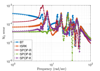
Figure 1: Comparison of the relative error magnitudes versus frequency in different methods when $r=15$.

Furthermore, when the outputs of BT or ISRK are taken as the initial points, Algorithm 1 presents better results than both BT and ISRK. This is because the projections generated by the BT and ISRK methods are generally not optimal in minimizing the approximation error, while the proposed scheme can take their outputs as initial points and leads to a local optimal projection via the iterations on the noncompact Stiefel manifold. Particularly, when $r=15$, SPOP-B and SPOP-K further reduce the relative errors by $41.0\%$ and $18.6\%$, compared to BT and ISRK, respectively. The detailed comparison of the approximation error magnitudes at different frequencies is presented in Fig. 1, which shows that the SPOP-B and SPOP-K methods outperform the BT or ISRK approaches for most frequencies, particularly in the lower frequency range. This shows the potential of the presented method as a posterior procedure of the balanced truncation or the Krylov subspace methods, as it is able to further improve the quality of the projection and hence gives a better reduced-order model.

5.2 Passivity-Preserving Model Reduction of Mass-Spring-Damper System

We further show the effectiveness of the proposed framework in the passivity-preserving model reduction problem for port-Hamiltonian systems, which has received considerable attention from the model reduction literature. We adopt the benchmark example of a mass-spring-damper system as shown in Fig. 2, with masses $m_{i}$, spring coefficients $k_{i}$ and damping constants $c_{i}$, $i=1,...,\ell$. The displacement of the mass $m_{i}$ is indicated by $q_{i}$. The same model parameters are used as in [19], which considers $\ell=50$ masses and hence $100$ states in the full-order model. Furthermore, the system inputs are two external forces $u_{1}$, $u_{2}$ applied to the masses $m_{1}$, $m_{2}$, whose velocities $\dot{q}_{1}$ and $\dot{q}_{2}$ are measured as the outputs $y_{1}$, $y_{2}$ of the system. We refer to [19] for the detailed state-space formulation of this mass-spring-damper system.

Figure 2: A mass-spring-damper system with $\ell$ masses has the dimension of $n=2\ell$.

To preserve the passivity of the full-order model, we let $X$ in (9) be chosen as the Hamiltonian matrix of the system, which satisfies the LMI (5). Our optimal projection approach in Algorithm 1, shortened as SPOP, is then compared with the other two projection-based methods, namely, the balanced truncation method for port-Hamiltonian systems (BT-PH) in [27], and the iterative tangential rational interpolation method (IRKA-PH) for port-Hamiltonian systems in [19]. In Algorithm 1, we fix the number iteration at $100$ and adopt the steepest descent strategy in (41) to compute a stepsize at each iteration. Furthermore, the starting point of the SPOP algorithm is initialized by one-step interpolation. Specifically, we choose sets of initial interpolation points $\{s_{1},...,s_{r}\}$ that are logarithmically spaced between $10^{-3}$ and $10^{-1}$ and tangential directions $\{b_{1},...,b_{r}\}$ as the dominant right singular vectors of the transfer matrix $G(s)$ at each interpolation point. Then an initial point is constructed as follows:

$$V_{0}=\begin{bmatrix}(s_{1}I-A)^{-1}Bb_{1},...,(s_{r}I-A)^{-1}Bb_{r}\end{bmatrix},$$ (52)

which is replaced with a real basis if the columns of $V_{0}$ occur in conjugate pairs, see [19] for more details. The same interpolation points and directions are used to initialize the IRKA-PH algorithm for comparison. We adopt each of the methods to reduce the full-order model to reduced ones with the order from $r=2$ to $r=20$. The resulting relative $\mathcal{H}_{2}$ errors for different reduced orders are illustrated in Fig. 3, from which we observe that the proposed method achieves superior performance to both BT-PH and IRKA-PH, especially when the reduced model dimension between $6$ and $16$. For instance, when $r=10$, our method achieves a relative error in the $\mathcal{H}_{2}$ norm that is $49.55\%$ and $46.96\%$ smaller errors than BT-PH and IRKA-PH, respectively. The convergence feature of the presented iterative method is illustrated by Fig. 4, in which we see a monotone decay of the objective function in each case when increasing the number of iterations. Eventually, the algorithm can gradually converge to a local optimum as shown in Fig. 4.

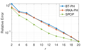
Figure 3: The magnitudes of the relative $\mathcal{H}_{2}$ errors as the reduced dimension $r$ varies.

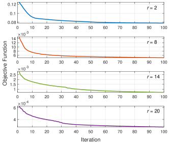
Figure 4: Comparison of the error magnitudes versus frequency in different methods when $r=15$.

Next, we illustrate both Algorithm 1 and Algorithm 2 in reducing a model with $\ell=1000$, i.e. $n=2000$ to a reduced-order model with $r=10$. In both algorithms, fixed stepsizes are imposed, i.e. $\alpha_{k}=0.21$ in Algorithm 1, and $\tau_{k}=0.21$ in Algorithm 2 at each iteration. Furthermore, we make a comparison between the two algorithms and the Riemannian trust-region method [40], where each algorithm is implemented for 100 iterations with the initial point as the output of IRKA-PH. Fig. 5 depicts the amplitude plot of the reduction errors, and Table 2 shows the relative $\mathcal{H}_{2}$ error and total running time on an Intel Core i7-7500U (2.70GHz) CPU.

From Fig. 5 and Table 2, we see that Algorithm 1 and Algorithm 2 achieve nearly the same approximation error, but Algorithm 2 requires more computation time since it requires the matrix inversion in (45) at each iteration. The Riemannian optimization approach does not impose the Petrov-Galerkin projection and thus achieves a better approximation compared to Algorithm 1 and Algorithm 2. However, it consumes more than three times the computation time of the proposed algorithms.

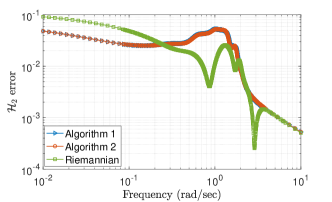
Figure 5: Comparison of the relative error magnitudes versus frequency in the three algorithms.

Table 2: Comparison of three algorithms with 100 iterations

Algorithms	Relative Error	Running Time
Algorithm 1	0.1616	99.46s
Algorithm 2	0.1618	109.34s
Method in [40]	0.1088	344.81s

6 Conclusions

In this paper, we have presented a novel model reduction method that incorporates nonconvex optimization with the Petrov-Galerkin projection, which provides a unified framework for reducing linear systems with different properties, including stability, passivity, and bounded realness. An optimization problem has been formulated on a noncompact Stiefel manifold, aiming to find an optimal projection such that the resulting approximation error is minimized in terms of the $\mathcal{H}_{2}$ norm. The gradient expression for the objective function is derived, which leads to a gradient descent algorithm that produces a locally optimal solution. The convergence property of the algorithm has also been analyzed. Finally, the feasibility and performance of the proposed method has been illustrated by two numerical examples, which shows that the method can be applied to both stability-preserving and passivity-preserving model reduction problems and can achieve smaller approximation errors compared to the existing balanced truncation and Krylov subspace approaches.

References

- [1] P.-A. Absil, R. Mahony, and R. Sepulchre. Optimization Algorithms on Matrix Manifolds. Princeton University Press, 2009.
- [2] D. S. A.C. Antoulas and S. Gugercin. A survey of model reduction methods for large-scale systems. Contemporary Mathematics, 280:193–219, 2001.
- [3] B. M. Afkham and J. S. Hesthaven. Structure-preserving model-reduction of dissipative Hamiltonian systems. Journal of Scientific Computing, 81(1):3–21, 2019.
- [4] A. C. Antoulas. Approximation of Large-Scale Dynamical Systems. SIAM, Philadelphia, USA, 2005.
- [5] A. C. Antoulas. A new result on passivity preserving model reduction. Systems & control letters, 54(4):361–374, 2005.
- [6] C. A. Beattie and S. Gugercin. Krylov-based minimization for optimal model reduction. In Proc. 46th IEEE Conference on Decision and Control, pages 4385–4390. IEEE, 2007.
- [7] C. A. Beattie and S. Gugercin. A trust region method for optimal model reduction. In Proc. 48h IEEE Conference on Decision and Control (CDC) held jointly with the 28th Chinese Control Conference, pages 5370–5375. IEEE, 2009.
- [8] P. Benner and P. Kürschner. Computing real low-rank solutions of Sylvester equations by the factored adi method. Computers & Mathematics with Applications, 67(9):1656–1672, 2014.
- [9] T. Breiten, R. Morandin, and P. Schulze. Error bounds for port-Hamiltonian model and controller reduction based on system balancing. Computers & Mathematics with Applications, 2021.
- [10] T. Breiten and B. Unger. Passivity preserving model reduction via spectral factorization. arXiv preprint arXiv:2103.13194, 2021.
- [11] B. Brogliato, R. Lozano, B. Maschke, O. Egeland, et al. Dissipative Systems Analysis and Control: Theory and Applications, volume 2. Springer, 2007.
- [12] X. Cheng and J. M. A. Scherpen. Model reduction methods for complex network systems. Annual Review of Control, Robotics, and Autonomous Systems, 4:425–453, 2021.
- [13] A. Edelman, T. A. Arias, and S. T. Smith. The geometry of algorithms with orthogonality constraints. SIAM journal on Matrix Analysis and Applications, 20(2):303–353, 1998.
- [14] G. Flagg, C. Beattie, and S. Gugercin. Convergence of the iterative rational Krylov algorithm. Systems & Control Letters, 61(6):688–691, 2012.
- [15] D. Goldfarb, Z. Wen, and W. Yin. A curvilinear search method for p-harmonic flows on spheres. SIAM Journal on Imaging Sciences, 2(1):84–109, 2009.
- [16] S. Gugercin. An iterative SVD-Krylov based method for model reduction of large-scale dynamical systems. Linear Algebra and Its Applications, 428(8-9):1964–1986, 2008.
- [17] S. Gugercin and A. C. Antoulas. A survey of model reduction by balanced truncation and some new results. International Journal of Control, 77(8):748–766, 2004.
- [18] S. Gugercin, A. C. Antoulas, and C. Beattie. model reduction for large-scale linear dynamical systems. SIAM Journal on Matrix Analysis and Applications, 30(2):609–638, 2008.
- [19] S. Gugercin, R. V. Polyuga, C. Beattie, and A. J. Van Der Schaft. Structure-preserving tangential interpolation for model reduction of port-Hamiltonian systems. Automatica, 48(9):1963–1974, 2012.
- [20] C. Guiver and M. R. Opmeer. Error bounds in the gap metric for dissipative balanced approximations. Linear Algebra and Its Applications, 439(12):3659–3698, 2013.
- [21] S.-A. Hauschild, N. Marheineke, and V. Mehrmann. Model reduction techniques for linear constant coefficient port-Hamiltonian differential-algebraic systems. arXiv preprint arXiv:1901.10242, 2019.
- [22] T. C. Ionescu and A. Astolfi. Families of moment matching based, structure preserving approximations for linear port-Hamiltonian systems. Automatica, 49(8):2424–2434, 2013.
- [23] R. Ionutiu, J. Rommes, and A. C. Antoulas. Passivity-preserving model reduction using dominant spectral-zero interpolation. IEEE Transactions on Computer-Aided Design of Integrated Circuits and Systems, 27(12):2250–2263, 2008.
- [24] K. Jbilou. Low rank approximate solutions to large Sylvester matrix equations. Applied Mathematics and Computation, 177(1):365–376, 2006.
- [25] Y.-L. Jiang and K.-L. Xu. Model order reduction of port-Hamiltonian systems by riemannian modified fletcher–reeves scheme. IEEE Transactions on Circuits and Systems II: Express Briefs, 66(11):1825–1829, 2019.
- [26] N. Jorge and J. W. Stephen. Numerical Optimization. Spinger, 2006.
- [27] Y. Kawano and J. M. Scherpen. Structure preserving truncation of nonlinear port-Hamiltonian systems. IEEE Transactions on Automatic Control, 63(12):4286–4293, 2018.
- [28] N. Kottenstette, M. J. McCourt, M. Xia, V. Gupta, and P. J. Antsaklis. On relationships among passivity, positive realness, and dissipativity in linear systems. Automatica, 50(4):1003–1016, 2014.
- [29] J. C. Meza. Steepest descent. Wiley Interdisciplinary Reviews: Computational Statistics, 2(6):719–722, 2010.
- [30] B. C. Moore. Principal component analysis in linear systems: Controllability, observability, and model reduction. IEEE Transactions on Automatic Control, 26(1):17–32, 1981.
- [31] T. Moser and B. Lohmann. A new Riemannian framework for efficient -optimal model reduction of port-Hamiltonian systems. In Proc. 59th IEEE Conference on Decision and Control (CDC), pages 5043–5049. IEEE, 2020.
- [32] G. Obinata and B. D. O. Anderson. Model Reduction for Control System Design. Springer Science & Business Media, 2012.
- [33] J. R. Phillips, L. Daniel, and L. M. Silveira. Guaranteed passive balancing transformations for model order reduction. IEEE Transactions on Computer-Aided Design of Integrated Circuits and Systems, 22(8):1027–1041, 2003.
- [34] R. V. Polyuga and A. J. Van der Schaft. Structure preserving model reduction of port-Hamiltonian systems by moment matching at infinity. Automatica, 46(4):665–672, 2010.
- [35] R. V. Polyuga and A. J. van der Schaft. Effort-and flow-constraint reduction methods for structure preserving model reduction of port-Hamiltonian systems. Systems & Control Letters, 61(3):412–421, 2012.
- [36] T. Reis and T. Stykel. Positive real and bounded real balancing for model reduction of descriptor systems. International Journal of Control, 83(1):74–88, 2010.
- [37] T. Sadamoto, A. Chakrabortty, and J.-i. Imura. Fast online reinforcement learning control using state-space dimensionality reduction. IEEE Transactions on Control of Network Systems, 8(1):342–353, 2020.
- [38] Z. Salehi, P. Karimaghaee, and M.-H. Khooban. A new passivity preserving model order reduction method: conic positive real balanced truncation method. IEEE Transactions on Systems, Man, and Cybernetics: Systems, 2021.
- [39] H. Sato. Riemannian Optimization and Its Applications. Springer, 2021.
- [40] K. Sato. Riemannian optimal model reduction of linear port-Hamiltonian systems. Automatica, 93:428–434, 2018.
- [41] K. Sato and H. Sato. Structure-preserving optimal model reduction based on the Riemannian trust-region method. IEEE Transactions on Automatic Control, 63(2):505–512, 2017.
- [42] P. Schwerdtner and M. Voigt. Structure preserving model order reduction by parameter optimization. arXiv preprint arXiv:2011.07567, 2020.
- [43] R. C. Selga, B. Lohmann, and R. Eid. Stability preservation in projection-based model order reduction of large scale systems. European Journal of Control, 18(2):122–132, 2012.
- [44] D. C. Sorensen. Passivity preserving model reduction via interpolation of spectral zeros. Systems & Control Letters, 54(4):347–360, 2005.
- [45] D. C. Sorensen and A. C. Antoulas. The sylvester equation and approximate balanced reduction. Linear Algebra and Its Applications, 351:671–700, 2002.
- [46] P. Van Dooren, K. A. Gallivan, and P.-A. Absil. -optimal model reduction of mimo systems. Applied Mathematics Letters, 21(12):1267–1273, 2008.
- [47] Z. Wen and W. Yin. A feasible method for optimization with orthogonality constraints. Mathematical Programming, 142(1):397–434, 2013.
- [48] J. C. Willems. Dissipative dynamical systems. European Journal of Control, 13(2-3):134–151, 2007.
- [49] T. Wolf, B. Lohmann, R. Eid, and P. Kotyczka. Passivity and structure preserving order reduction of linear port-Hamiltonian systems using krylov subspaces. European Journal of Control, 16(4):401–406, 2010.
- [50] Y. Wu, B. Hamroun, Y. Le Gorrec, and B. Maschke. Reduced order lqg control design for port-Hamiltonian systems. Automatica, 95:86–92, 2018.
- [51] M. Xia, P. J. Antsaklis, V. Gupta, and F. Zhu. Passivity and dissipativity analysis of a system and its approximation. IEEE Transactions on Automatic Control, 62(2):620–635, 2016.
- [52] S. Xie, L. Xie, and C. E. De Souza. Robust dissipative control for linear systems with dissipative uncertainty. International Journal of Control, 70(2):169–191, 1998.
- [53] K.-L. Xu, Y.-L. Jiang, and Z.-X. Yang. order-reduction for bilinear systems based on Grassmann manifold. Journal of the Franklin Institute, 352(10):4467–4479, 2015.
- [54] W.-Y. Yan and J. Lam. An approximate approach to optimal model reduction. IEEE Transactions on Automatic Control, 44(7):1341–1358, 1999.
- [55] L. Yu and J. Xiong. model reduction for negative imaginary systems. International Journal of Control, 93(3):588–598, 2020.
- [56] C. Zheng, Y. Tan, J. T. Wen, and A. M. Maniatty. Finite element model based temperature consensus control for material microstructure. In Proc. American Control Conference (ACC), pages 619–624. IEEE, 2015.